The Use of Lower or Higher Heating Value, Heat Release Rate and Heat Loss in Internal Combustion Engines

Abstract

The heat release rate in internal combustion engines obtained from in-cylinder pressure data is a fundamental method to analyse the combustion characteristics of engines. As the measured in-cylinder pressure is lower than the pressure in the absence of heat loss to the walls, the methodology typically leads to the apparent rate of heat release as the heat loss to the cylinder walls cannot be segregated. Heat loss can then be inferred by reference to the chemical fuel energy expected to be released by the fuel. Typically, in engine thermodynamic analysis, the lower heating value is used to determine the energy released by the fuel. However, in this article, we argue that when detailed comparison with validated combustion modelling was done, it was concluded that the higher heating value is the more appropriate calorific value. In this research, the analysis of heat release rate and its determination using the first law of thermodynamics with constant ratio of specific heats $\gamma$ and also varying $\gamma$ is discussed. It was noted that the use of the “3rd term” (term due to the $d\gamma /d\mathsf{\vartheta }$) in the heat release rate is advisable as it gives a more reasonable heat loss even in the compression stroke.

1. Introduction

Heat loss from the working fluid to the cylinder walls in an internal combustion engine is an energy loss whose understanding is sought and whose magnitude should preferably be reduced. The energy lost by the working fluid due to heat transfer to the walls reduces the available energy of the working fluid and therefore negatively impacts the amount of energy converted to useful mechanical work.

The understanding of the combustion process has long been given attention as exemplified by Rassweiler & Withrow [1] whose analyses are still very widely used to determine the mass fraction burned (MFB) profile. Obert [2] states that Schweitzer used the tangent method for analysis of indicator cards of internal combustion engines and proposed a method to calculate “heat addition” as early as 1926. The rate of heat release is typically done by the method that builds on the first law and the ideal gas law. Amann [3] gives a review on the use of in-cylinder pressure and mentions that in 1906 Clerk used the first law with pressure-Volume (pV) data whilst motoring down an engine to determine heat loss. Obert [2] discussed the heat release rate (HRR) determined from the first law of thermodynamics in both the spark ignition (SI) and compression ignition (CI) combustion which do have differences as in SI the mixture of fuel is premixed while in CI it is direct injected. Obert makes numerous references to the works by Kreiger and Borman [4,5,6] all of whom (including Obert) hailed from University of Wisconsin Madison. Even as early as the 1960s, it is evident from the works of Kreiger and Borman and others that they were using the super computers of the time (2 min for compile and run time for one diesel engine cycle on CDC 1604) to better analyse engine performance. Obert does not mention whether the heat coming from the fuel is related to the lower heating value (LHV) or the higher heating value (HHV). Krieger [4] does mention LHV of the gasoline fuel as only a descriptive term not because it is used in equations. Krieger’s main aim was to calculate the mass fraction burned profile and used the Eichelberg correlation to calculate and account for heat transfer. A curious result in Krieger’s paper is that the mass fraction burned profiles presented for both diesel and gasoline fuel combustion show mass fraction with crank angle profiles that do not taper slowly to unity at the end of combustion (like the Wiebe function) but hit unity at a high angle.

Later, in his book of the 1980s, Heywood [7] also treats heat release in both the contexts of SI and CI. An equation for the apparent heat release based on the first law is given in [7] (Equation (1) below). Heywood also presents a diagram that gives a very vivid explanation of the crank angle history of the released chemical fuel energy ($m_f{Q}_{LHV}$), the apparent heat release, the heat transfer and combustion inefficiency, all indicated in this diagram ([7] Figure 9.12). The diagram can be traced to come from Gatowski ([8] Figure 5) who had worked under the supervision of Heywood. Gatowski proposed and used a linear equation for gamma, hence Gatowski was using variable specific heats and hence variable gamma. Later, Shudo [9,10,11,12], gave an equation for the apparent heat release also based on the first law but accounted for the variation in gamma by including a third term (Equation (2) below). Shudo referred to this additional term in the HRR in many of his publications and commented that the “3rd Term”, i.e., the term which has $d\gamma /d\mathsf{\vartheta }$, is very important in hydrogen engines unlike other cases such as in typical hydrocarbon engines.

$${\displaystyle \frac{d{Q}_{net}\left(\theta \right)}{d\theta }}={\displaystyle \frac{\gamma }{\gamma -1}}·p\left(\theta \right)·{\displaystyle \frac{dV\left(\theta \right)}{d\theta }}+{\displaystyle \frac{1}{\gamma -1}}·V\left(\theta \right)·{\displaystyle \frac{dp\left(\theta \right)}{d\theta }}$$

(1)

$${\displaystyle \frac{d{Q}_{net}\left(\theta \right)}{d\theta }}={\displaystyle \frac{\gamma }{\gamma -1}}·p\left(\theta \right)·{\displaystyle \frac{dV\left(\theta \right)}{d\theta }}+{\displaystyle \frac{1}{\gamma -1}}·V\left(\theta \right)·{\displaystyle \frac{dp\left(\theta \right)}{d\theta }}-{\displaystyle \frac{1}{{\left(\gamma -1\right)}^2}}pV·{\displaystyle \frac{d\gamma }{d\theta }}$$

(2)

In Gatowski’s paper [8], the “3rd term” is not given in a form that is in any way similar to that given by Shudo. The same equation given by Shudo is also given in the Ansys^® Forte manual [13] (albeit, to date, the Forte manual has a wrong sign in front of the “3rd term”). In Heywood [7], the chemical energy of the fuel is always attributed to LHV never HHV. In Gatowski [8], the difference in internal energy of the products and reactants is stated as related to LHV but no reason is given. More recently the gross heat release was studied by Lanzafame [14] who also noted the strong influence of the ratio of specific heats.

Shayler [15,16], more specifically in the 1993 paper, used different versions of the HRR (i.e., constant gamma and variable properties) and showed that the calculated HRR and subsequently heat loss have great dependency on the variation in properties. Shayler says, “Small differences in the net heat transferred result in large differences in the predicted heat loss to the chamber”. Shayler ends up saying that due to the inherent large changes in calculated heat loss based on the selected gamma, it leads to little confidence in this method. Surprisingly, Shayler et al. end up suggesting it is better to rely on heat loss to the coolant and the heat loss to exhaust in order to calculate heat loss. Shayler [16] specifically mentions LHV, so it is not ambiguous. Shayler also uses the fact that heat loss by first law of thermodynamics goes negative in order to discredit that method. But the figure referred to in Shayler’s analysis ([16] Figure 1) has a note that manifold absolute pressure (MAP) was 411 mbar (40 kPa) therefore very close to idle. The engine capacity 2.0 L, RPM and torque were also given which translate to 4.4 kW. Therefore, the low MAP and low torque indicate the engine was therefore practically motoring. In earlier studies, Wendland [17] and Lawton [18], had analysed heat transfer in motoring condition and the negative heat flux was noted and explained as being the re-expansion of the boundary layer. In a related manner, the fact that the peak of the heat transfer to the wall arrived prior to the peak temperature used to be an anomaly. But Pfriem [19] had shown that the heat transfer would lead (in time) the temperature and which he termed “the compression heat” and used a complex (i.e., complex number $e^{i\theta }$) convective heat transfer coefficient which can handle the phase shifting between temperature and heat flux. Independently from Pfriem’s work, Wendland [17] developed an adiabatic plane model, modelling the combustion chamber as a number of gas laminae from the cylinder mid-plane and he also reported the phase difference between the heat transfer and temperature and referred to it as the “pressure work”.

Shayler refers to Alkidas [20] as a reference on heat flux measurements and noted that Alkidas did not report negative heat flux. However, it can be noted that in Alkidas heat flux peaks around TDC (actually in Alkidas heat flux peak is at 370 crank angle). In his paper, Alkidas also used the first law energy balance method to calculate the heat loss during the valve closed period, but Alkidas does not say if LHV or HHV were used. Shayler also refers and uses the method by Chun [21] (student of Heywood). Chun mentions chemical energy released in his analysis but does not specify in his text whether it was LHV or HHV. However, Chun indicated LHV in his figure ([21] Figure 1).

In recent works relating to the use of hydrogen in internal combustion engines, the high heat transfer capability of hydrogen and its small quench layer have led researchers to analyse the heat loss. Some have calculated the heat loss as the difference between the chemical fuel energy and the apparent heat release [9,10,11,12,22,23,24]. Beccari [24] made a detailed numerical analysis based on an extensive experimental data set obtained on a CFR engine (at 900 RPM) in which the air to fuel ratio and compression ratio were varied. Beccari used the term Heat Loss Efficiency (HLE), which is the ratio of fuel chemical energy less the apparent heat released divided by the apparent heat released, hence less heat loss if higher HLE and shows that hydrogen at λ = 2 had higher HLE than gasoline at λ = 1 and gasoline had higher HLE than methane at λ = 1. Beccari also showed that HLE was unaffected by compression ratio (CR).

Hydrogen use in internal combustion engines is also being researched in the simultaneous combined combustion of fuels (one of which hydrogen) to lower CO₂ emissions. Pukalskas [25] injected up to 30% energy content of hydrogen in low pressure (5 bar) port injected spark ignition gasoline engine. Shao [26] used a mixture of ammonia and hydrogen. Hydrogen was direct injected at pressures ranging from 40 to 80 bar. Willens [27] used a diesel pilot injection to start the combustion of the hydrogen direct injected fuel. Diesel fuel was injected at a rather low pressure of 290 bar, specifically stated to be 10 bar higher than the direct injection pressure of hydrogen at 280 bar to make sure no hydrogen goes back into the diesel system. However, by far, the most prominent use of dual-fuel combustion is that of diesel and methane [28,29].

Ricardo in his lengthy 1922 SAE paper [30] said that “it is generally agreed by engineers and scientists that the useful calorific value of a fuel is its total heat-value less the latent heat of evaporation of the water formed. It is customary, therefore, to reckon the efficiency on the basis of this lower calorific value, and it is legitimate to do so, because the temperature cannot be extended sufficiently in an ordinary cycle to make any use of the heat of condensation of steam” ([30] p. 6). This remark by Ricardo we believe is still valid today. However, we do now also believe that the determination of heat losses (including other effects such as blowby and combustion inefficiency) from the subtraction of the apparent heat release from the fuel chemical energy should not be based on the LHV but rather on the HHV. The authors argue that from a logical perspective, when the fuel is burning, there is no way the chemical reaction can “predict” how far the expansion process will be and hence whether the water molecules formed in the combustion process will be able to condense or not. Since it is actually possible that the combustion products are cooled to a low enough temperature that the water vapor is condensed, such as in the bomb calorimeter (albeit not an engine), the release of combustion energy is associated with the HHV. Therefore, the authors believe that for a thermal efficiency calculation it is fair to use LHV but for heat losses the HHV should be used.

The authors have come to this conclusion aided or rather compelled by the detailed combustion simulations performed using ANSYS^® Forte (version 2024 R2) mainly for dual-fuel combustion (diesel/methane and diesel/propane) but have also noticed this when analysing other in-cylinder pressure data from another test engine using hydrogen and petrol.

The following sections in this article present experimental results collected using a dual-fuel engine operated in diesel only mode and dual-fuel mode. In dual-fuel mode the main fuel charge (gaseous fuel) was methane or propane and the pilot fuel was diesel. The experimental in-cylinder pressure was also reproduced using combustion simulations in ANSYS Forte. Analytical thermodynamic analysis of the heat release based on the experimental in-cylinder pressure was conducted using different methods including the Rassweiler & Withrow method, and the first law method with constant gamma and variable gamma. The results of heat release were compared to that obtained through the simulation results. This analysis was done with the aim to provide a reference on different methods of experimental data post-processing for heat release and wall heat transfer analysis. The research was done on two modes of combustion namely diesel compression-ignition combustion and dual-fuel combustion which incorporates autoignition and flame propagation combustion phenomena.

2. The Dual-Fuel Engine Experimental Setup

The experimental data was obtained from a dual-fuel engine. Dual-fuel engines mostly operate on diesel and natural gas (methane being the major constituent) and have advantages relating to lower exhaust emissions and also provide the operational flexibility to switch completely to diesel if methane supply is low. Dual-fuel engines produce less emissions of particulate matter because the quantity of diesel injected is less compared to diesel only operation and the gaseous component of the fuel does not result in particulate matter when combusted. Furthermore, dual-fuel engines produce less CO₂ emissions because the gaseous fuel has a higher hydrogen to carbon ratio than diesel and thus a lower quantity of carbon participates in the combustion [31]. Dual-fuel engines have become widely used in the marine industry where the natural gas is stored in liquid form (Liquified Natural Gas, LNG).

2.1. Experimental Setup

The engine used for the experimental investigation in this study was a PSA DW10, 2 L common rail diesel engine that was converted to dual-fuel operation in previous work [32]. The basic engine specifications are presented in Table 1. The engine was operated in diesel-only (DO) mode and dual-fuel (DF) mode. In dual-fuel mode, the engine was supplied with gaseous fuel injected into the air intake manifold and diesel pilot injected directly in the cylinder close to top dead centre. The quantity of diesel supplied in DO mode and DF mode was kept the same. In DF mode, the addition of gaseous fuel thus increased the output power of the engine. The reason for keeping the same quantity of diesel in both DO and DF modes was intentional to enable the isolation of the diesel combustion from the dual-fuel combustion phenomena during setup phase of simulation work.

Table 1. Engine specifications.

Cylinder quantity	4
Bore (mm)	85
Stroke (mm)	88
Displacement (L)	1.9974
Compression ratio	18

Both propane and methane were used as the gaseous fuel in DF mode, thus presenting two variants for DF mode, namely DF-methane (diesel-methane) and DF-propane (diesel-propane). The storge of propane was in liquified petroleum gas form and methane was in compressed gas form (cylinder at 200 bar). All tests were conducted at an engine speed of 2000 RPM, as this is the engine speed at which the engine experiences the optimal volumetric efficiency and thus maximum torque.

2.2. LabVIEW Data Acquisition and Post Processing

LabVIEW™ 2021 software was used to acquire and post-process the experimental data. The aim was to analyse the combustion characteristics of the CI engine whilst operating in DO and DF mode. The crank angle resolved data was acquired at 0.1 crank angle degree interval using a crank mounted BEI shaft encoder (H25D-SS-3600-ABZC-28V/OC-SC18) that also had a one pulse per revolution signal, Z-index. In-cylinder, crank angle resolved, pressure data was acquired along with other channels namely: z-index, current through the diesel injector coil and current through the gas injector coil. The diesel injector coil current trace was used to confirm the Duration of Injection (DOI) and confirm the Start of Injection (SOI). The gas injector current trace was used to confirm the DOI of the gaseous fuel injector. The crank angle resolved data is referred to here as the fast data to differentiate it from the slow data that was recorded at 10 Hz. The slow speed data at 10 Hz was also acquired using LabVIEW software to record slow speed parameters such as engine torque, mass air flow, coolant temperature, exhaust gas temperature, exhaust gas lambda sensor, NOx emissions, etc., which were measured directly by National Instruments™ (NI) DAQ. The slow speed DAQ also logged parameters from the ECU GUI data stream (by sniffing) such as engine speed, manifold absolute pressure (MAP), DOI, SOI, coolant temperature etc.

An AVL GH14P pressure transducer, installed in the glow plug port of one cylinder, was used to measure in-cylinder pressure (Pressure range: 0–150 bar; Sensitivity: 15.43 pC/bar; Linearity: ±0.11%). The output signal was fed to a charge amplifier (AVL, Graz, Austria, Flexifem Piezo Type 2P2G). TDC position was determined by using the motoring data and allowing for loss angle [33]. The in-cylinder pressure obtained from the piezo electric sensor was pegged to the MAP at Inlet Valve Close (IVC). One hundred and fifty (150) cycles at each test point were recorded and used for analysis. The fast data was acquired using a National Instruments USB-6363 card and saved using TDMS file format. The slow speed data was acquired using an NI PCI 6229 Card connected to an SXCI module that provided signal conditioning closer to the measurement. A NI USB 8502 CAN bus module was used to sniff data between the Reata Engineering ECU and the GUI computer. Real time knock monitoring was done using a MoTec (Melbourne, Australia) M600 ECU and a MoTec knock module. Slow data from the Motec ECU to the Motec GUI computer (via CAN bus) was also integrated into the slow speed data. The slow speed data was saved in Comma Separated Values format.

3. Combustion Simulation

Combustion simulations for both DO and DF engine operation were done in ANSYS^® Forte (version 2024 R2) which performs coupled CFD-combustion simulations. This section describes the overall model setup and further details are described in Saliba [34]. Table 2 indicates the models used for turbulence, diesel injection spray droplet break up and heat transfer.

Table 2. Simulation models.

	Model
Turbulence	RANS RNG $\kappa$-$\epsilon$
Spray droplet break up	Kelvin-Helmholtz/Rayleigh-Taylor (KH/RT)
Heat transfer	Amsden

The engine cylinder geometry was represented by a 72° sector given the diesel injector had five nozzles. The mesh was built in ANSYS Forte using automatic mesh generation feature with a base cell size of 3 mm and solution adaptive mesh on temperature, velocity, vapour and G-equation.

Combustion reactions were represented by the use of a detailed chemical kinetic mechanism to calculate species production rates and concentrations. The Rahimi et al. mechanism [35] was used for DO combustion simulations. A reduced version of the ANSYS Model Fuel Library gasoline mechanism [36] was used for the DF combustion simulations. Diesel was represented by n-heptane in both DO and DF simulations.

The Autoignition-Induced Flame propagation model (AIF) was used to control the switch from ignition kernel to flame propagation model. The flame propagation was modelled using the G-equation model. The laminar flame speed was determined from the built-in flame speed tables.

The Amsden heat transfer model in conjunction with the temperature law-of-the-wall boundary condition was used. The Amsden model was originally implemented in KIVA-3V code [37] and is also available in ANSYS Forte. The Amsden heat transfer model is an isothermal wall heat transfer model, which assumes a constant near-wall temperature, density and Prandtl number within the boundary layer.

4. Analysis

4.1. Mass Fraction Burned

The Rassweiler & Withrow (R&W) method was used to determine the mass fraction burned (MFB). This method needs a starting point and an end point for calculation. The starting point was taken as the angle of SOI while the end point was initially taken as Exhaust Valve Open (EVO) but then modified accordingly to coincide with the angle where the peak MFB occurred. The MFB was used to determine the Accumulated Heat Release (AHR) by multiplying the energy content of the fuel and accounting for a combustion efficiency (described later in Section 6). The Heat Release Rate (HRR) was determined by taking the derivative of the AHR.

4.2. Apparent Heat Release Rate (aHRR)

The apparent Heat Release Rate (aHRR) was determined using the widely used Equation (1) (presented earlier and also derived in Appendix A.1) which is obtained by considering the gases within the trapped volume as a single bulk and applying the Fist law of Thermodynamics.

The aHRR was also determined using Equation (2) which is obtained from the same stating points of Equation (1) but allowing for the variation in gamma with crank angle. Equation (2) has a third term that is the term which accounts for the variation in gamma with crank angle. This HRR equation in this form is given in the Shudo articles [9,10,11,12] and also in the Forte User’s Manual. The derivation of Equation (2) is included in Appendix A.2.

The accumulated heat release (AHR) was determined from the aHRR through integration.

5. Variation in Gamma

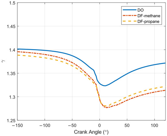
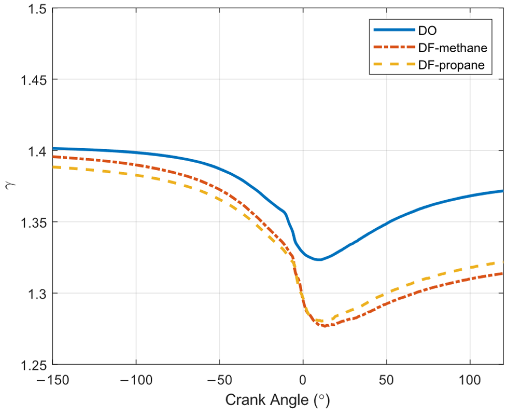
Chun’s paper [21] is mostly on determining gamma as a variable, and the complexity is appreciated. Methods used to estimate gamma in previous work is summarized in [38]. In the present work, the value for gamma used in Equation (2) was obtained from the ANSYS Forte simulation results. The values of gamma with crank angle are presented in Figure 1 for DO and the two DF modes. It may be observed that during intake valve close (−150° ATDC) the value for gamma in DO mode is close to 1.4 since the trapped gas in the cylinder is air. In the DF modes the addition of methane or propane in the intake air stream decreased the value for gamma. Furthermore, the variation in gamma with crank angle is appreciable and is due to the change in temperature and also the formation of combustion products. The range of crank angle is presented from −150° ATDC to 120° ATDC which are the Inlet Valve Close (IVC) and Exhaust Valve Open (EVO) respectively.

Figure 1. Gamma with crank angle from ANSYS Forte combustion simulations.

6. Experimental and Simulation Results

The in-cylinder pressure for Diesel Only (DO) operation as well as Dual-Fuel (DF) operation were acquired experimentally and then simulated in Ansys Forte (version 2024 R2). The engine operating conditions are reported in Table 3. Both the DO and the DF modes of operation reported here are at 2000 RPM, 150 kPa manifold absolute pressure and intake air temperature of 31–38 °C. The DO operation had a diesel fuel quantity of 0.01 g/injection (one injection pulse per cycle per cylinder) which was the result of a DOI of 0.3 ms at 750 bar rail pressure. The SOI was −15° ATDC (i.e., 15° BTDC). This condition is relatively low load, and the relevant Indicated Mean Effective Pressure (IMEP) was 3.7 bar. The DF conditions used the same quantity of diesel but in addition also had the gaseous fuel injection in the intake air manifold. The DF experiments were conducted using propane or methane as the gaseous fuel. The gas fuel flow rate, substitution ratio and IMEP are reported in Table 3. In this article, the DF cases are referred to as the high load due to the higher IMEP. In DF operation the diesel quantity was kept the same as in DO mode and the addition of the gaseous fuel therefore increased the power output of the engine when compared to DO operation. The diesel quantity and injection properties were kept the same in both DO and DF modes intentionally so that diesel injection properties and combustion characteristics could be simulated in isolation in DO simulation work and kept the same during DF simulation work.

Table 3. Engine operating conditions.

	DO	DF-Propane	DF-Methane
RPM	2000	2000	2000
MAP (kPa)	150	150	150
MAF (g/s)	68	65	60
Intake air temperature (°C)	35–38	36	31–32
Rail pressure (bar)	750	750	750
DOI (ms)	0.3	0.3	0.3
Diesel (g/injection)	0.01	0.01	0.01
SOI (° ATDC)	−15	−15	−15
Gaseous fuel flow rate (g/s)	0	1.5	1.75
Gaseous fuel/air equivalence ratio		0.36	0.5
Substitution Ratio (SR)	0	0.71	0.75
IMEP (bar)	3.7	10.7	12.5

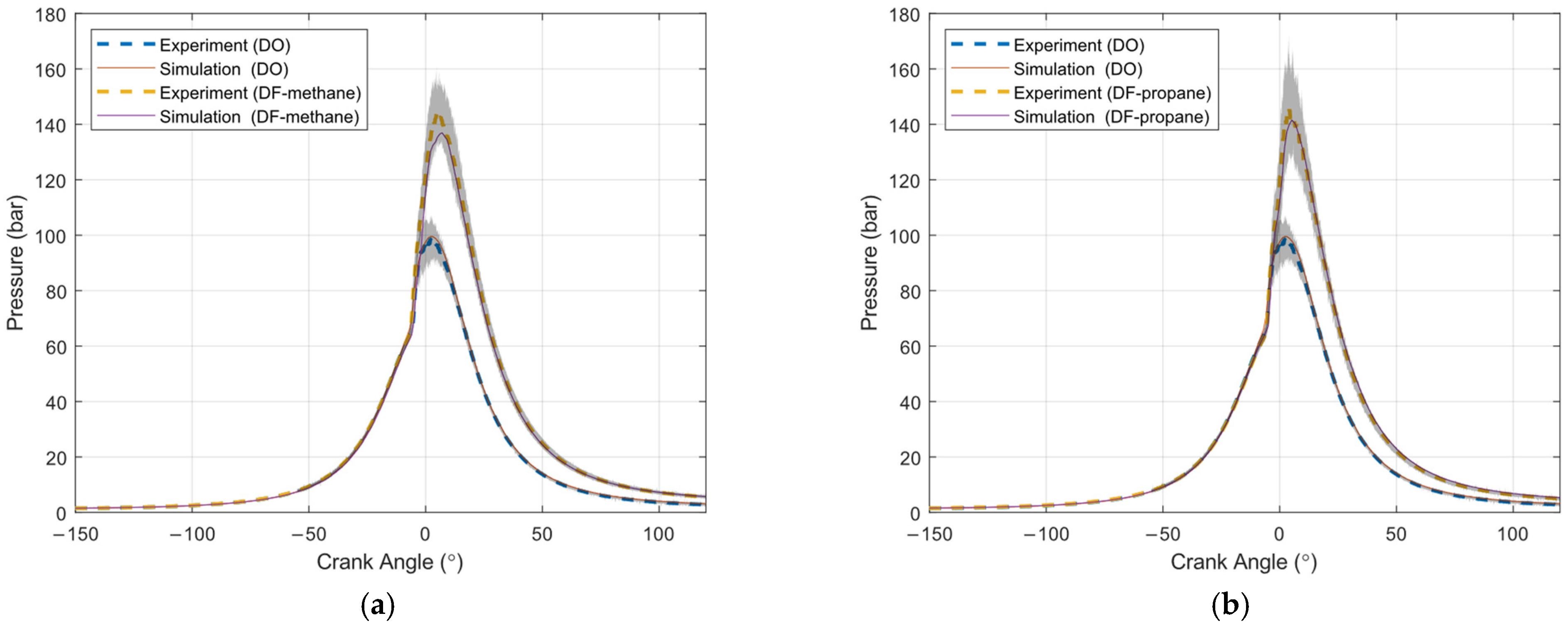
Figure 2a,b show the crank angle resolved experimentally measured in-cylinder pressure and the simulation results for both DO and DF operation, with methane and propane respectively. The experimental data is represented as ensemble average of 150 cycles and the grey area represents the maximum and minimum in-cylinder pressure experienced across the experimental cycles. The simulation in-cylinder pressure is presented superimposed and shows good agreement with the ensemble average pressure for all fuel combinations used.

Figure 2. Experimental and simulation in-cylinder pressure. (a) DO and DF-methane, (b) DO and DF-propane.

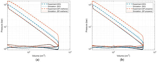
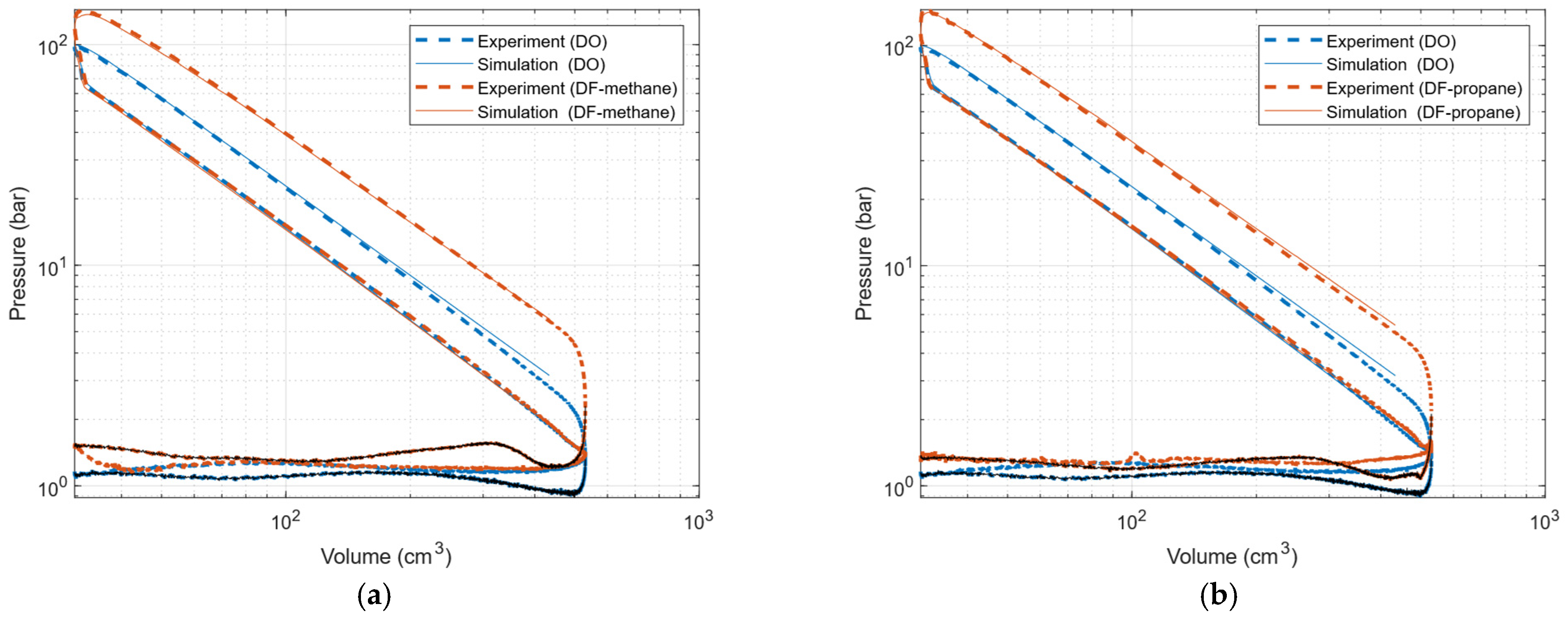
The p-V diagrams of the same operating conditions from both experimental and simulation results are presented in Figure 3. Figure 3a presents the p-V diagram for the DO and DF operation with the DF utilizing methane, i.e., the same data as in Figure 2a, while Figure 3b corresponds to the propane use in the DF operation i.e., the same data as in Figure 2b. Once again it is noted that there is excellent agreement in the experimental and simulation pressure data when plotted in log-log p-V diagrams.

Figure 3. p-V diagrams for DO and DF modes. (a) DO and DF-methane, (b) DO and DF-propane.

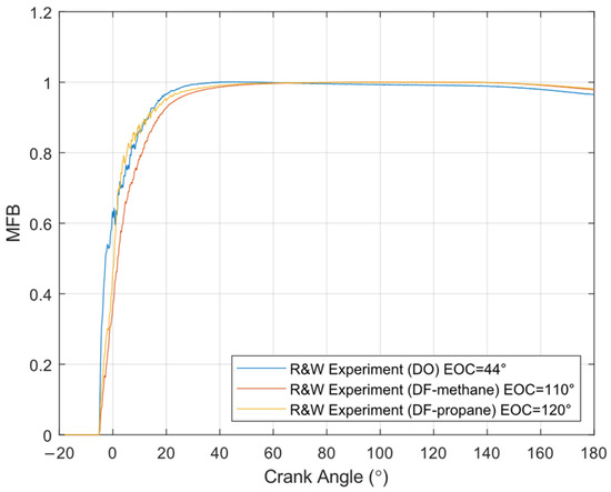
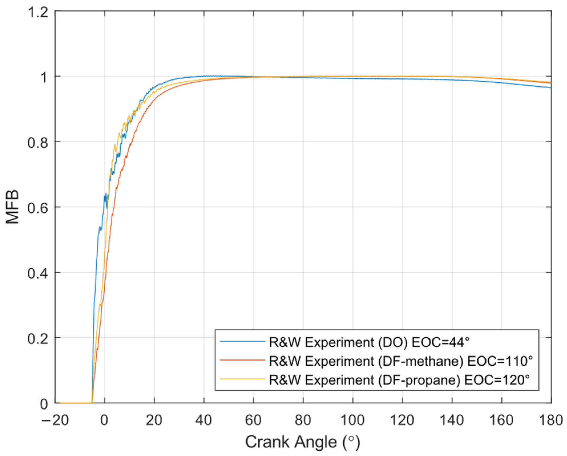
The experimental MFB was determined using the Rassweiler & Withrow method on the ensemble average in-cylinder pressure of the respective 150 consecutive cycles and is presented in Figure 4. The end of combustion (EOC) for the DO operation was set at 44° ATDC while the EOC for the DF operation was set at 110° ATDC and 120° ATDC for methane and propane DF respectively. The EOC was set by iteratively changing the EOC value to scale the max MFB to unity. The start of combustion in the Rassweiler & Withrow calculation was taken to be equal to the SOI. It is noted that the curves have a rapid initial burn rate for both DO and DF. In addition, the DF curves have slower latter portion of the combustion phase.

Figure 4. Mass fraction burned using Rassweiler & Withrow method on experimental data.

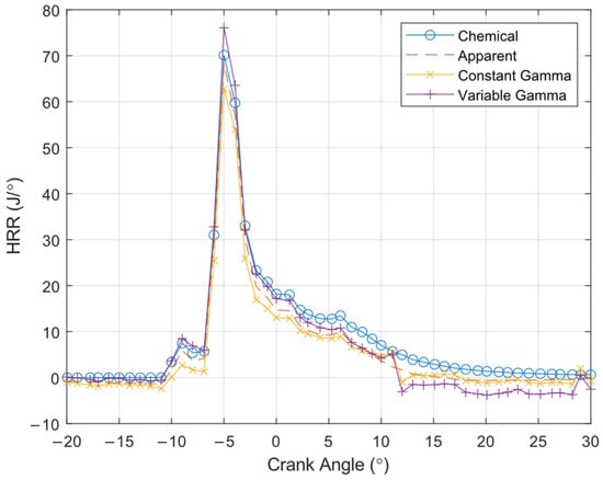
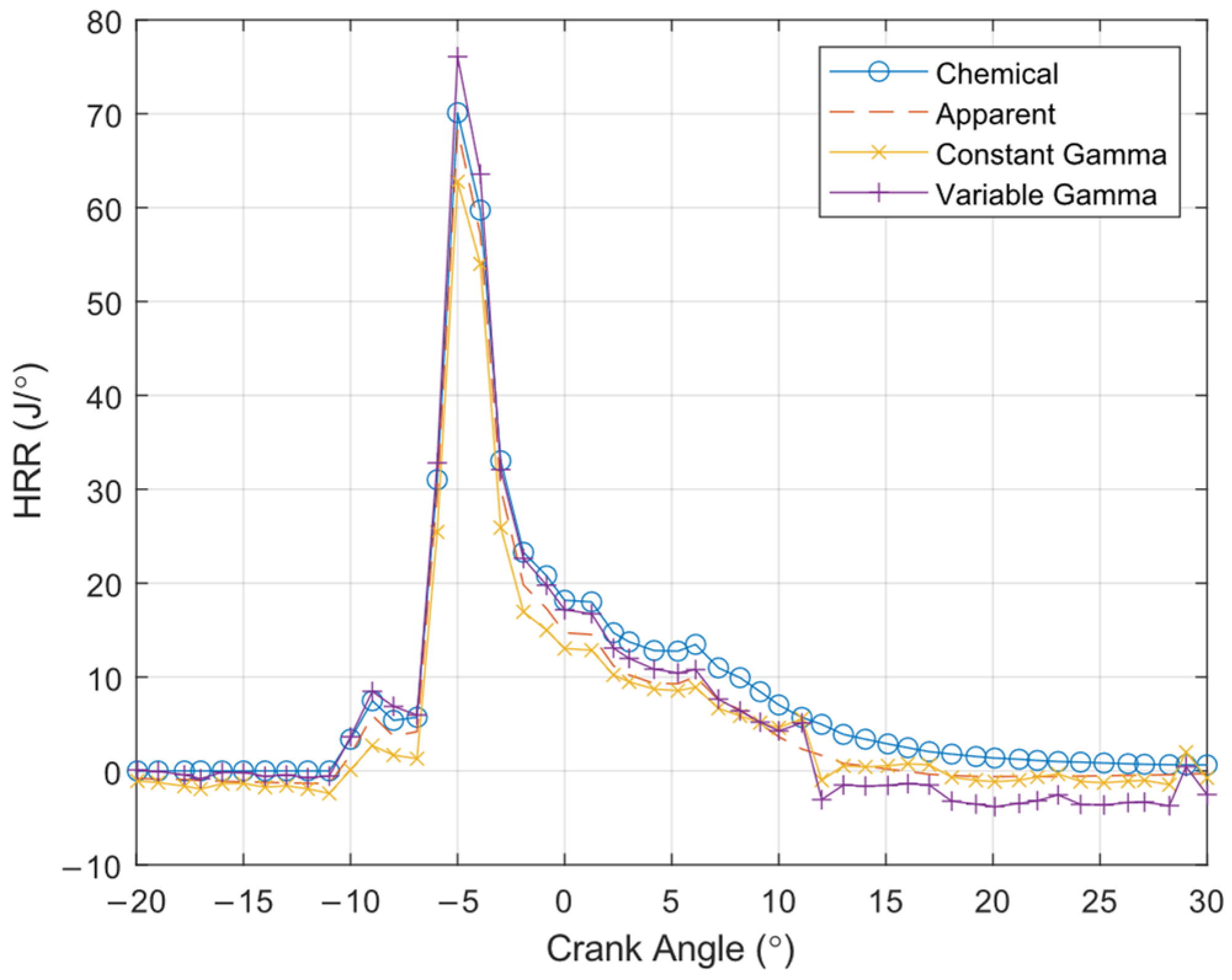
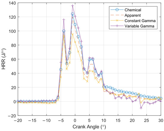
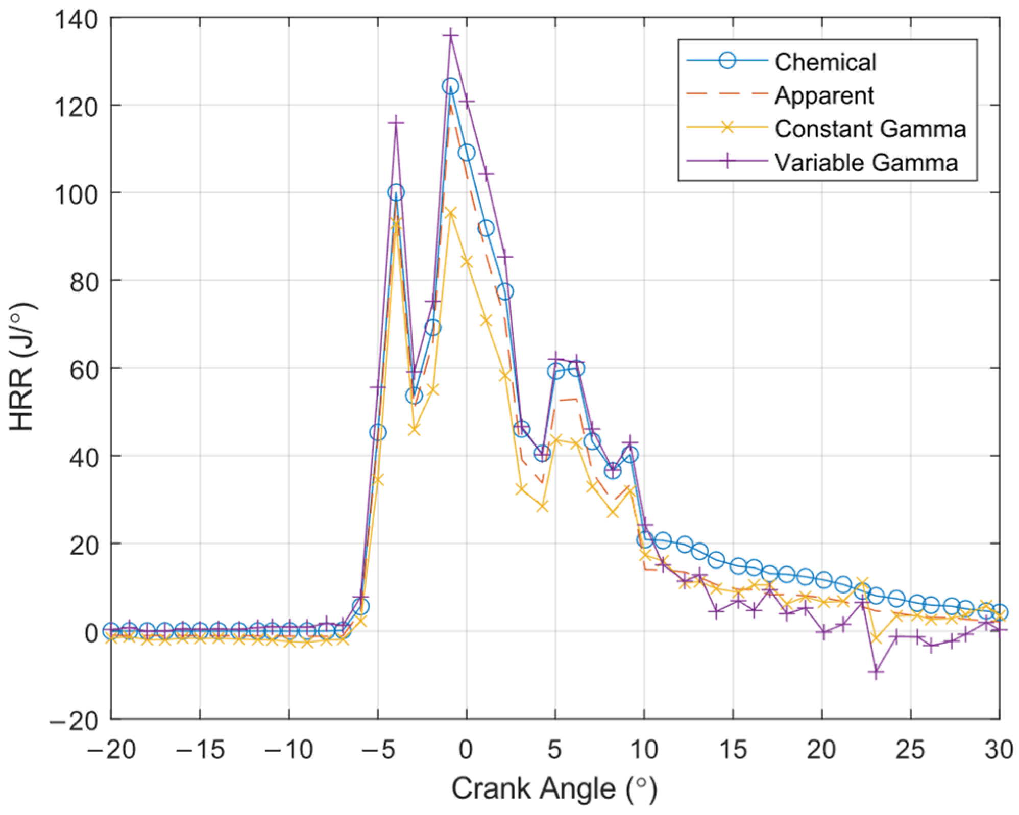
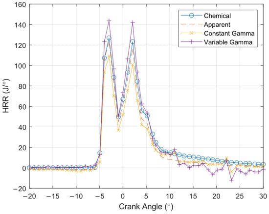
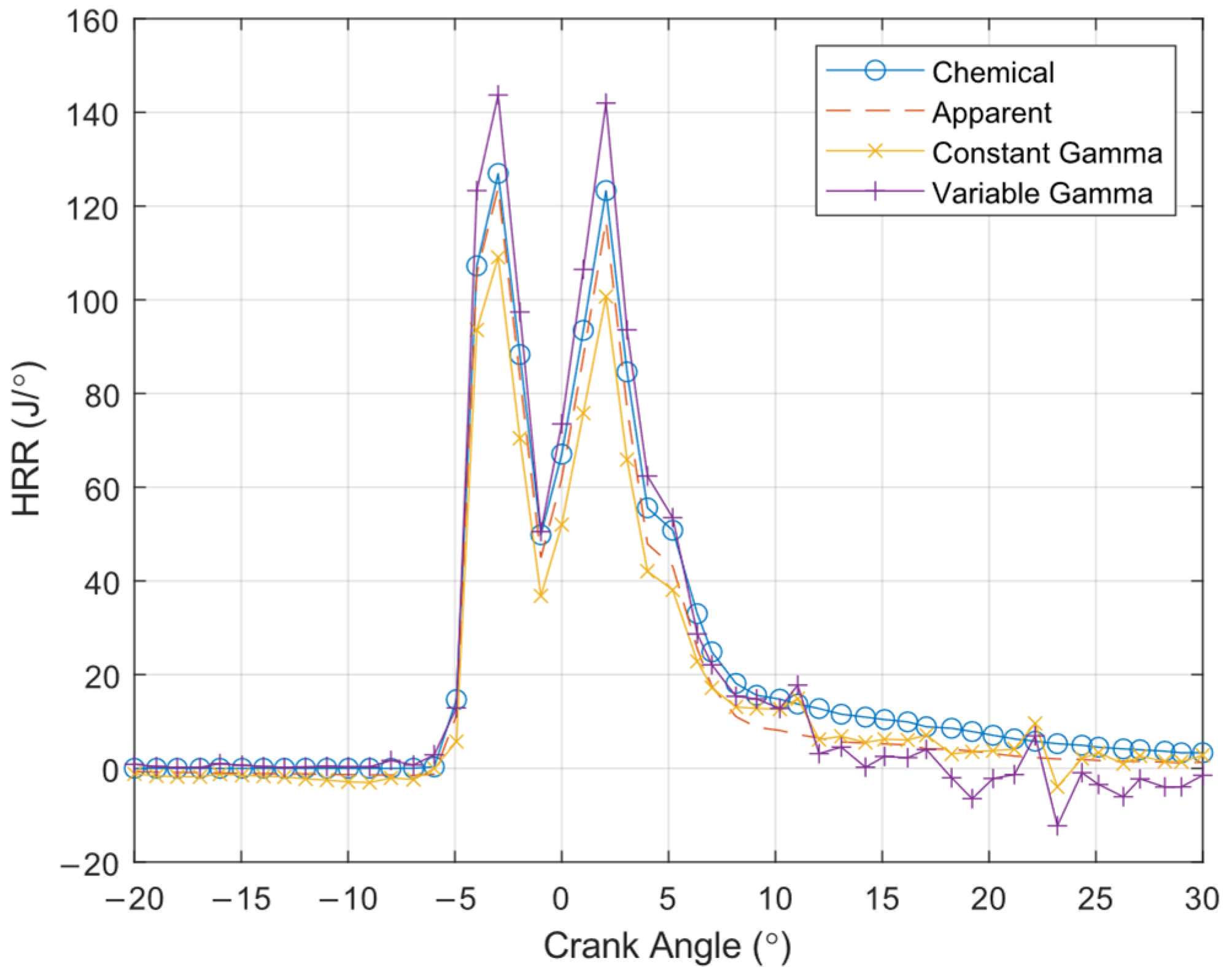
The HRR from the ANSYS Forte combustion simulations for DO, DF-methane and DF-propane are presented in Figure 5, Figure 6 and Figure 7 respectively. Forte presents different versions of HRR as plotted in the mentioned figures, including HRR from chemical data, HRR from p-V results using constant gamma (calculated using Equation (1)) and HRR from p-V results using variable gamma (calculated using Equation (2)). It is noted that the chemical HRR in Forte results is determined directly from the chemical energy coming from the combustion reactions. The fuel and chemistry characteristics defined in Forte are the fuel type, chemical composition and the chemical kinetics mechanism while neither LHV nor HHV is an input value. In Figure 5, Figure 6 and Figure 7 the apparent HRR as provided by Forte is presented. The apparent HRR as computed by Forte is the chemical HRR less the heat losses through the walls (where the heat losses are computed by Forte on a crank angle basis based on the Amsden heat transfer model between the cylinder gases and the cylinder liner, piston and head). Therefore, the apparent HRR in Figure 5, Figure 6 and Figure 7 is not the typically implied apparent HRR obtained from in-cylinder pressure data. The apparent HRR as computed by Forte and the experimental apparent HRR as typically computed by Equation (1) (or Equation (2) for that matter) are intrinsically related but are based on completely different starting points. While Figure 5, Figure 6 and Figure 7 do show differences in the constant gamma and variable gamma HRR plots, the differences are not very evident and discussion on the differences from the HRR plots is difficult.

Figure 5. Simulation HRR for DO mode.

Figure 6. Simulation HRR for DF-methane mode.

Figure 7. Simulation HRR for DF-propane mode.

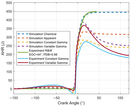
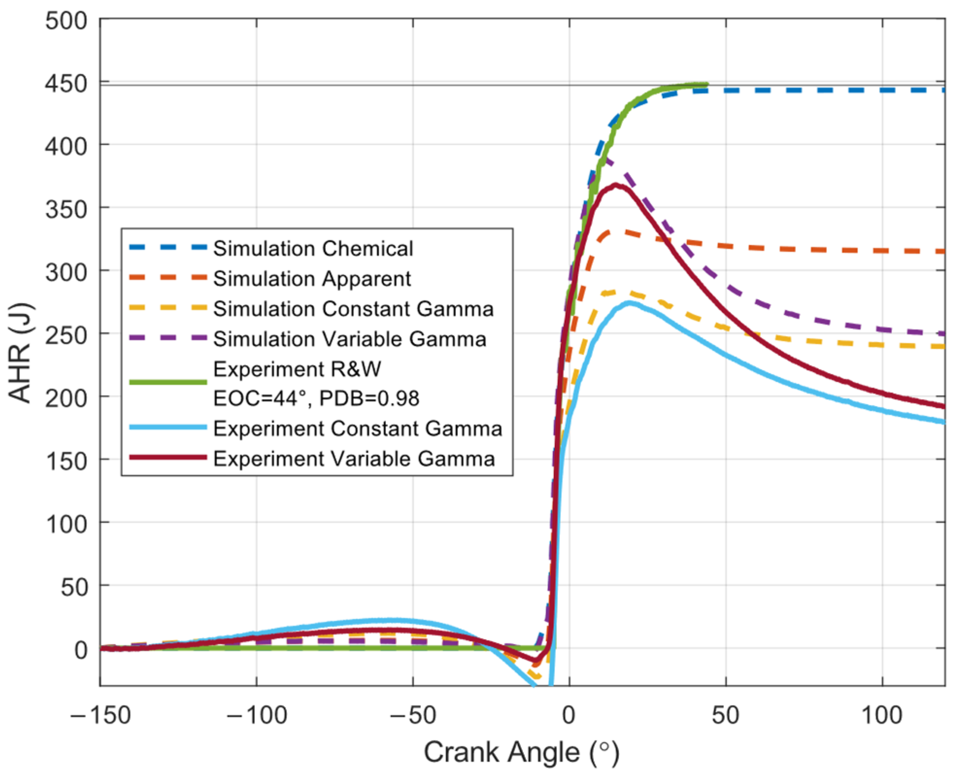
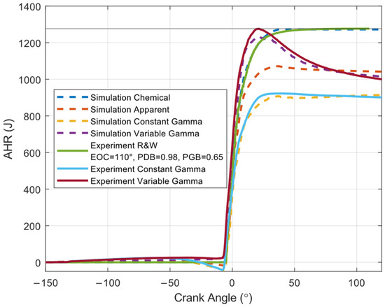
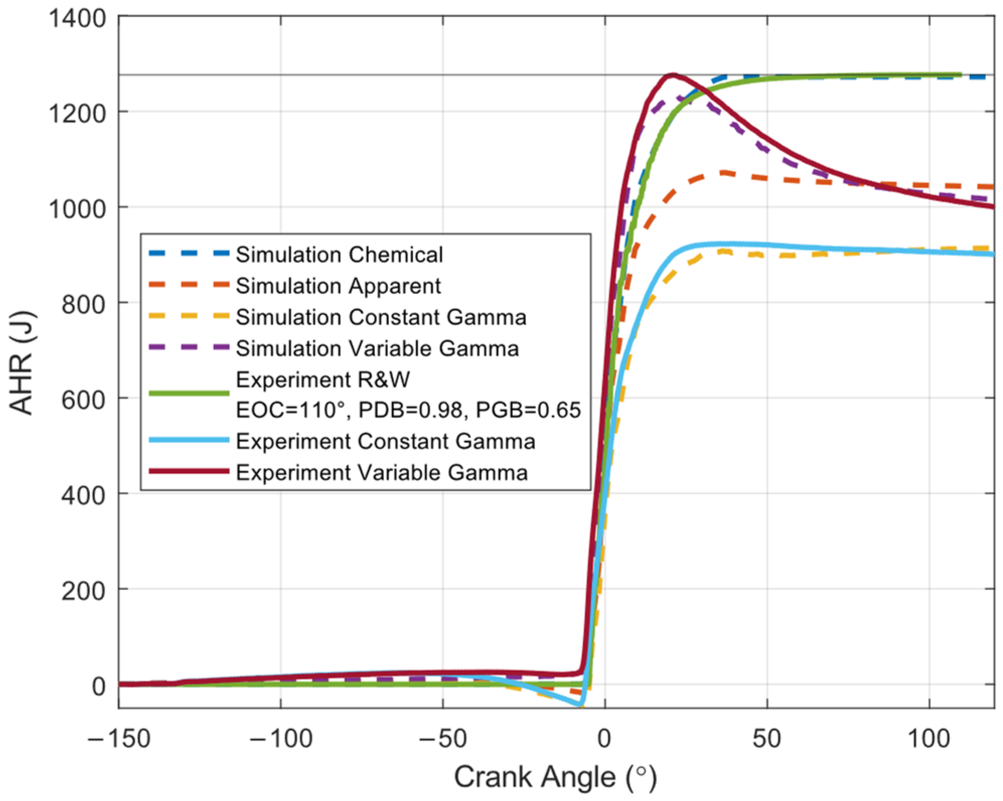
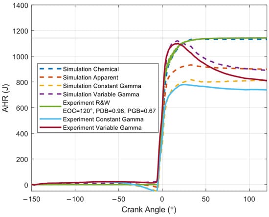
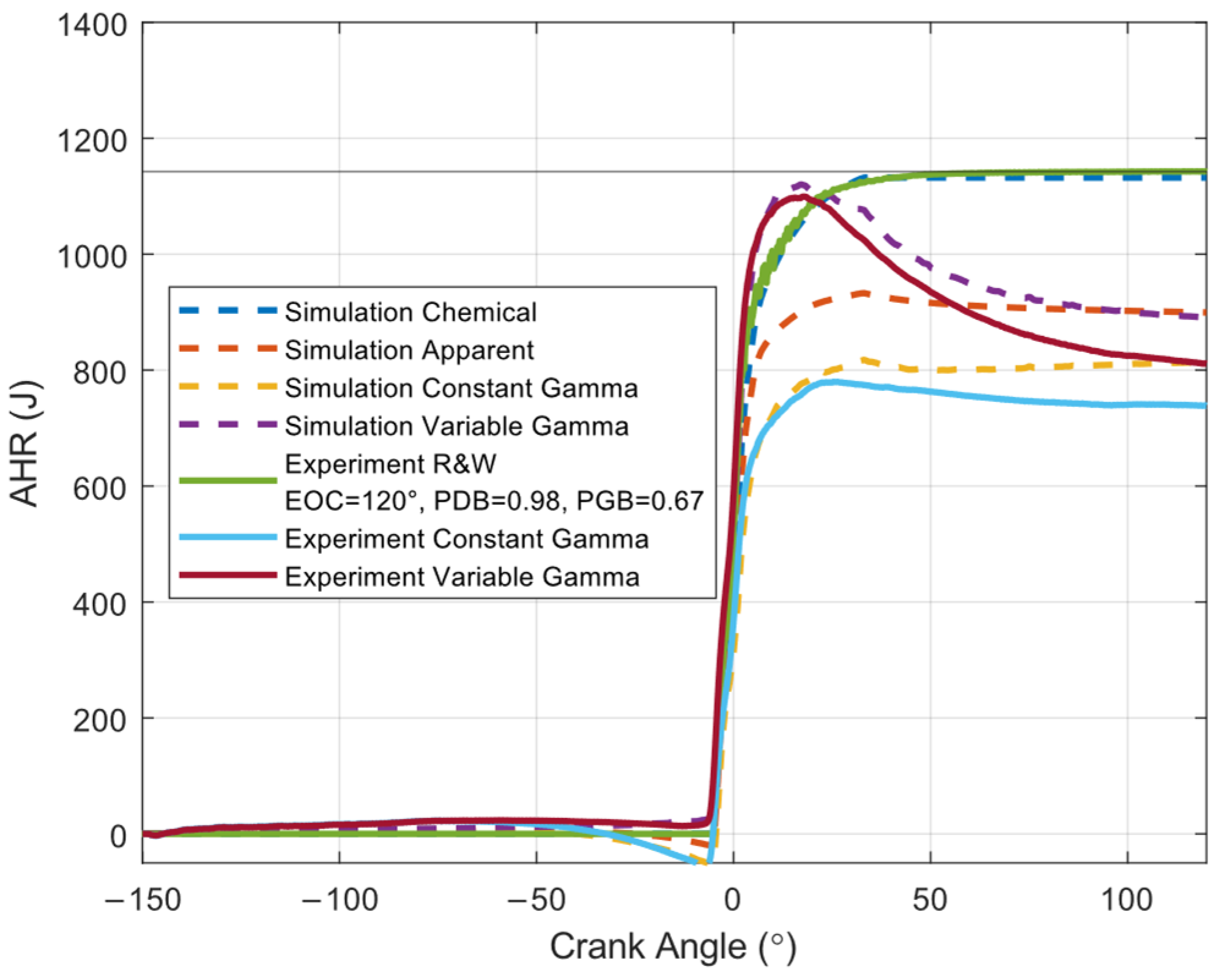
The effects of constant gamma and variable gamma is better viewed in the accumulated heat release (AHR), obtained by integrating the HRR. Figure 8, Figure 9 and Figure 10 show the AHR of the DO, DF-methane and DF-propane operation. From these figures it can be noted that as expected the chemical AHR is higher than the AHR obtained by both the constant gamma and variable gamma methods. It is noted that the constant gamma method has a noticeable dip, going considerably negative, before the steep rise in AHR. The variable gamma AHR has a much smaller dip and therefore the authors believe that this is an indication that the variable gamma methodology is a much better method. This is in line with suggestions by Krieger, Shudo, Gatowski, etc. that the variation in properties has a considerable effect and should be accounted for.

Figure 8. Experimental and simulation AHR for DO mode.

Figure 9. Experimental and simulation AHR for DF-methane mode.

Figure 10. Experimental and simulation AHR for DF-propane mode.

Figure 8, Figure 9 and Figure 10 also present the AHR curves obtained through the Rassweiler & Withrow method by multiplying the MFB by the energy content of the fuel. The main discussion point here (first focusing on DO case Figure 8) is that the Rassweiler & Withrow curves (which are intrinsically from zero to unity) needed to be multiplied by the HHV, the mass of fuel injected and the combustion efficiency to get this good agreement with the chemical AHR from Forte in Figure 8 for the DO case. The combustion efficiency employed in this calculation was 98% for the diesel combustion (Portion of Diesel Burned, PDB) which is a typical value [7]. When the Rassweiler & Withrow MFB was multiplied by the LHV and the mass of fuel, there was not a good agreement as the LHV is considerably lower than HHV. In fact, the value of mass of fuel multiplied by LHV is 417 J (0.01 g × 42.6 kJ/g × 0.98 = 417 J) which in fact is lower than the maximum chemical heat release shown in Figure 8 of 443 J. If HHV is considered the value obtained is 446 J, (0.01 g × 45.6 kJ/g × 0.98 = 446 J), which is closer to the maximum chemical heat release shown in Figure 8. The mass of fuel multiplied by HHV represents, in the authors’ opinion, the full fuel potential (0.01 g × 45.6 kJ/g = 456 J). If the maximum value of chemical heat release from Forte (443 J) is divided by the full fuel potential (456 J), the resulting combustion efficiency is 97%. This fact is being shown here on the DO operation, but the authors have investigated and seen similar requirement to multiply with HHV on other experimental data from a single cylinder engine operated on petrol and hydrogen [39].

For the DF mode with premixed air-fuel (methane or propane) the combustion efficiency employed for the gaseous fuel (Portion of Gas Burned, PGB) was 65% and 67% for methane and propane respectively in order to achieve good agreement between the simulation chemical AHR and the experimental R&W AHR. The diesel combustion efficiency was kept the same as that presented in DO mode (98%). The combustion efficiency for the gaseous fuel is considerably lower than the diesel portion or typical combustion efficiency in spark ignited petrol engines due to the lean fuel-air mixture used in the dual-fuel combustion, having λ values of 2 or higher, at which the tendency for flame termination is higher. Low combustion efficiency in DF operation was already the subject of a previous investigation where literature showed the challenges of high unburned hydro carbons in DF applications, and it was subsequently shown that the implementation of a throttle body in the intake had the potential of lowering the level of unburned hydro carbons [40]. Beccari ([24], Figure 9) showed that even for hydrogen, combustion efficiency dropped from 95% at lambda 1.3 to 85% at lambda 2 and 80% at lambda 2.2.

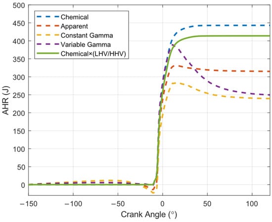
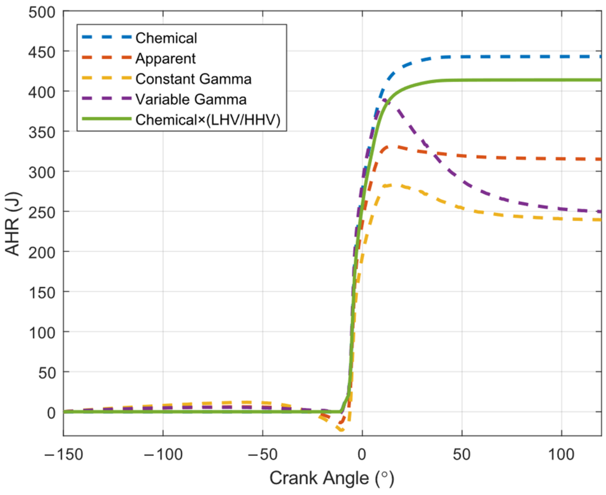
Figure 11 is presented to demonstrate the relative difference between HHV and LHV based on AHR in the DO operation. In this figure the simulation chemical AHR (blue dashed line) is also presented scaled by the ratio (LHV/HHV) which consequently lowers the maximum AHR plateau (green line). With reference to the numerical value determined above from 0.01 g × 42.6 kJ/g × 0.98 = 417 J, the green line plateaus at 414 J. On the other hand, the chemical heat release determined by Forte (i.e., the blue dashed line), plateaus at 443 J. This is higher than the value of mass of fuel multiplied by LHV (417 J) meaning that the combustion efficiency would actually be bigger than 100%, (443/417) which is surely not realistic and shows that the chemical heat released is equivalent to the HHV.

Figure 11. Simulation AHR for DO mode.

Figure 11 also gives a graphical representation of the gap between the variable gamma AHR and the chemical AHR. It is evident that the gap, which represents the heat loss is smaller if the LHV value is used compared to using the HHV. Therefore, the authors believe that when using the first law on the trapped mass of the working fluid to determine the heat loss (as done by many researchers including Shayler [16] and Alkidas [20]) the HHV should be used if no access to combustion simulations is available. This has the effect that the heat losses determined will be of a bigger value if based on HHV compared to LHV. Applying the HHV would have prevented Shayler [16] from reporting the aforementioned negative heat losses at the onset of expansion, or at least mitigated the magnitude and frequency of this phenomenon.

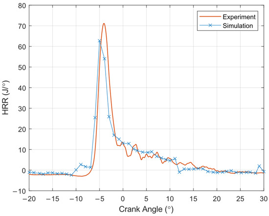
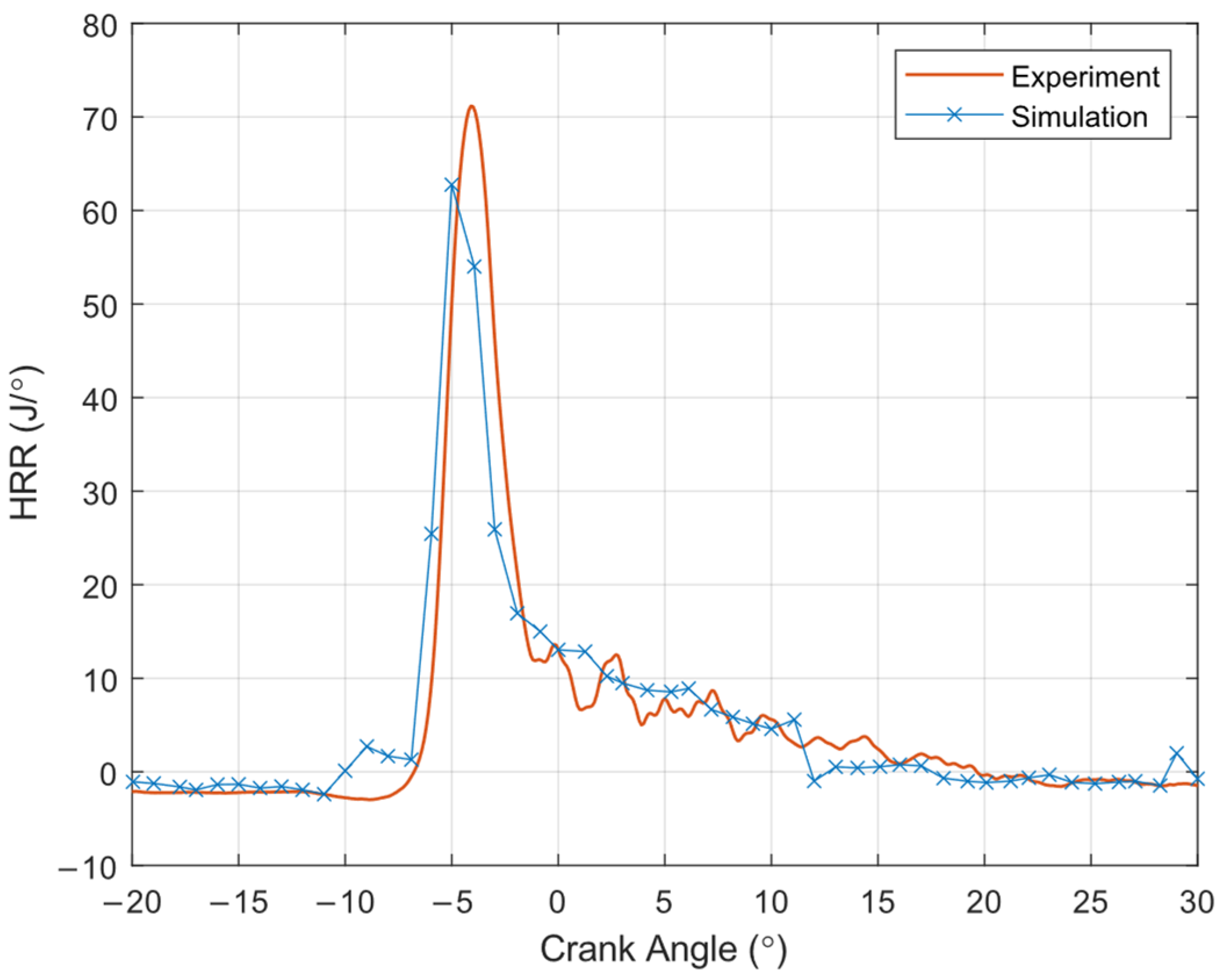
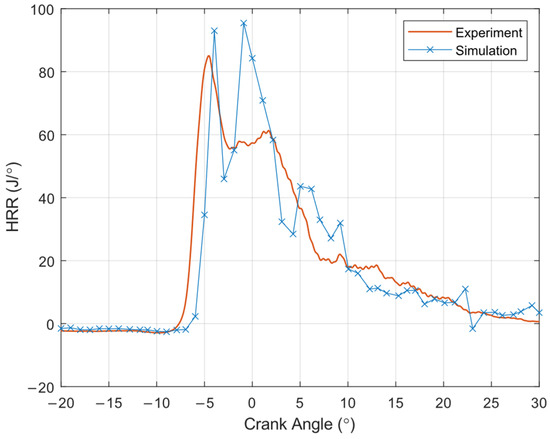
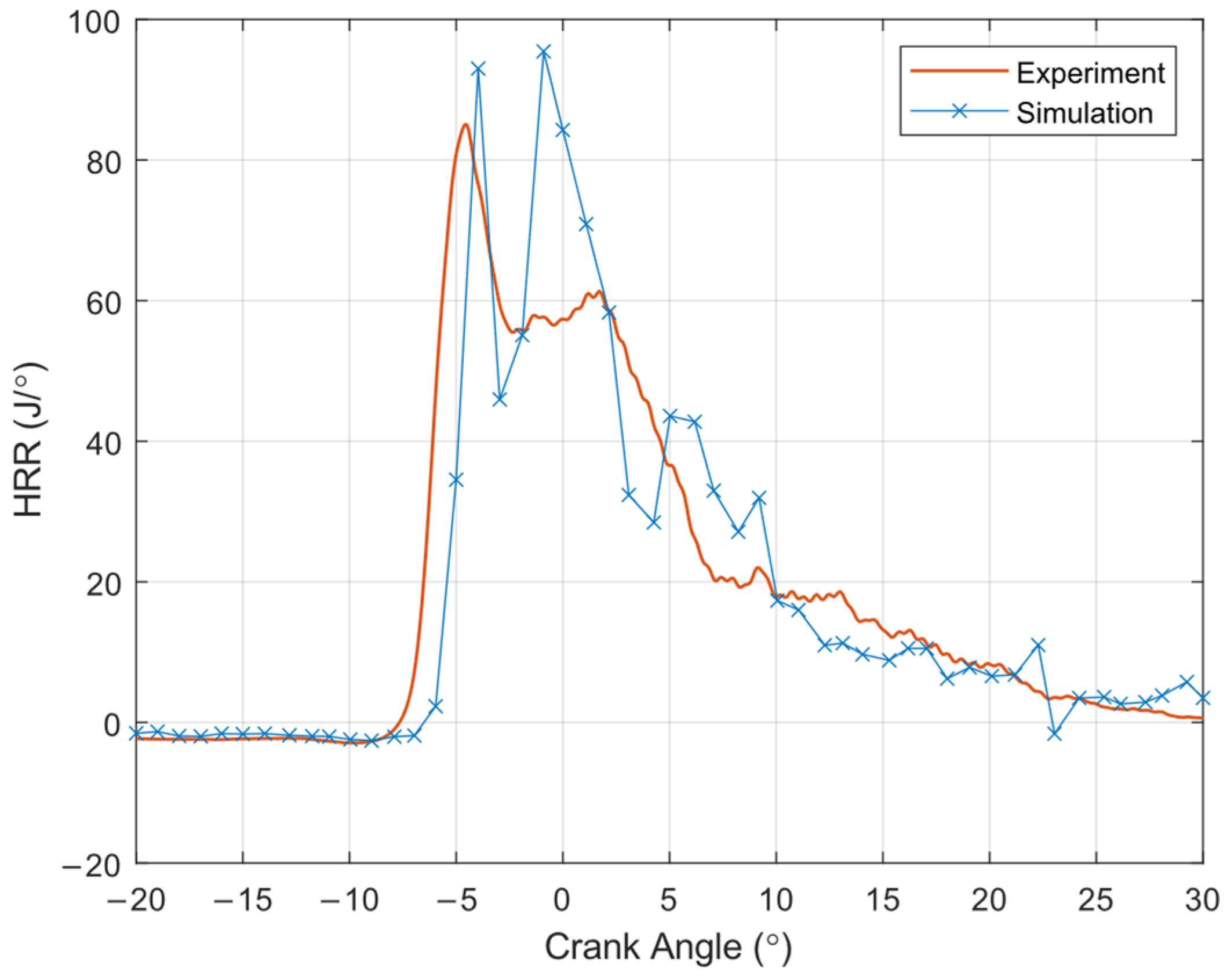
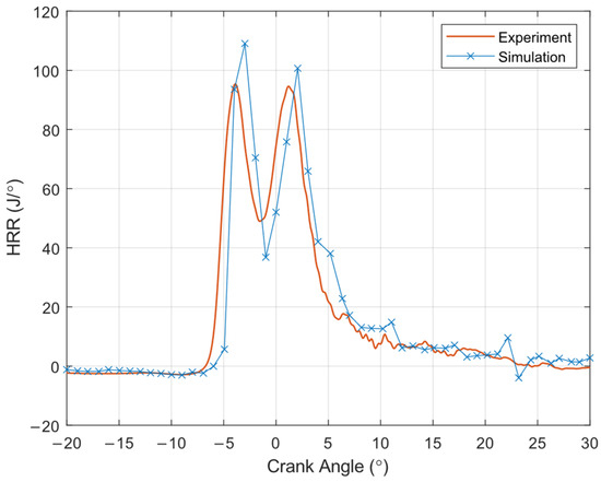
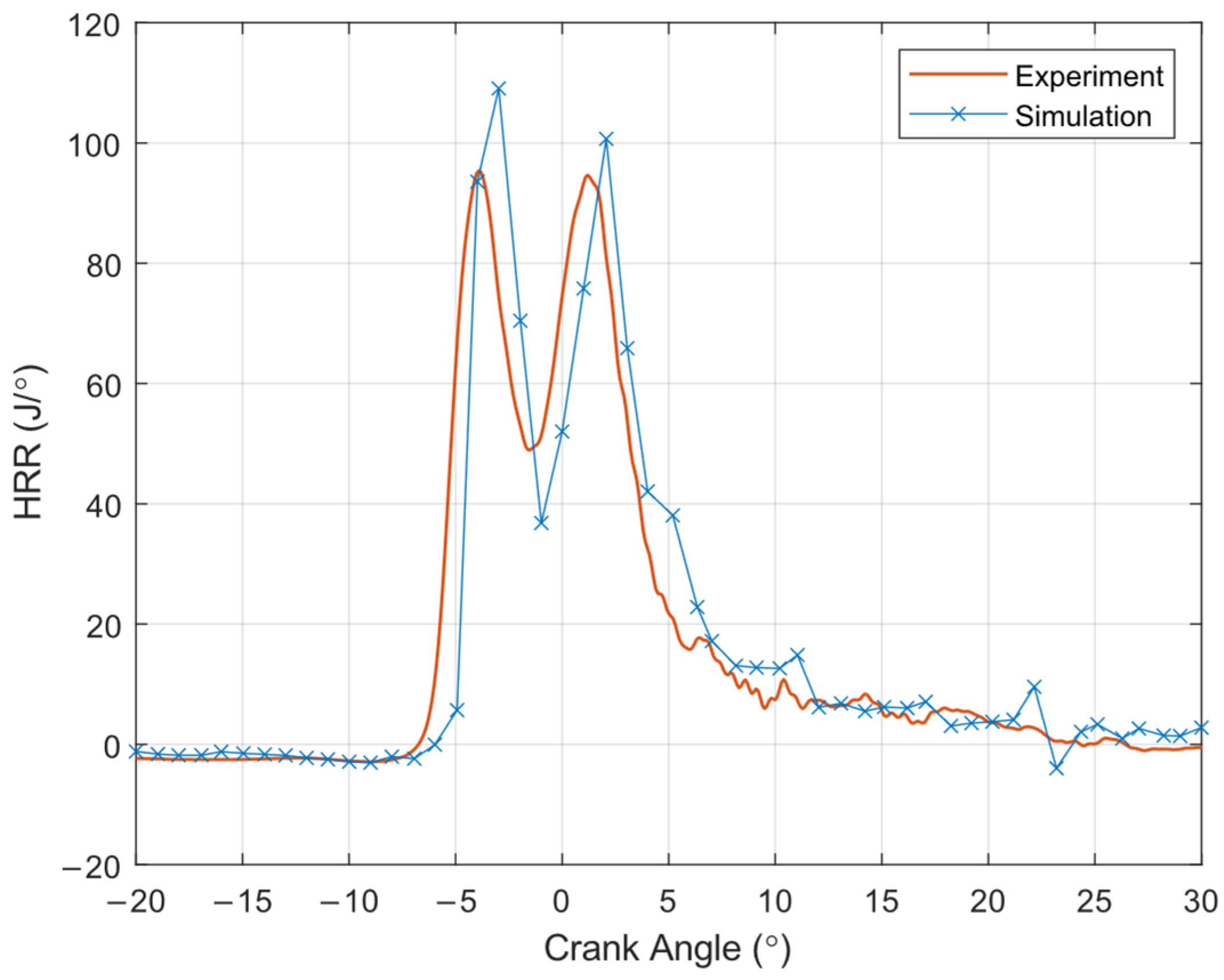
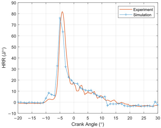
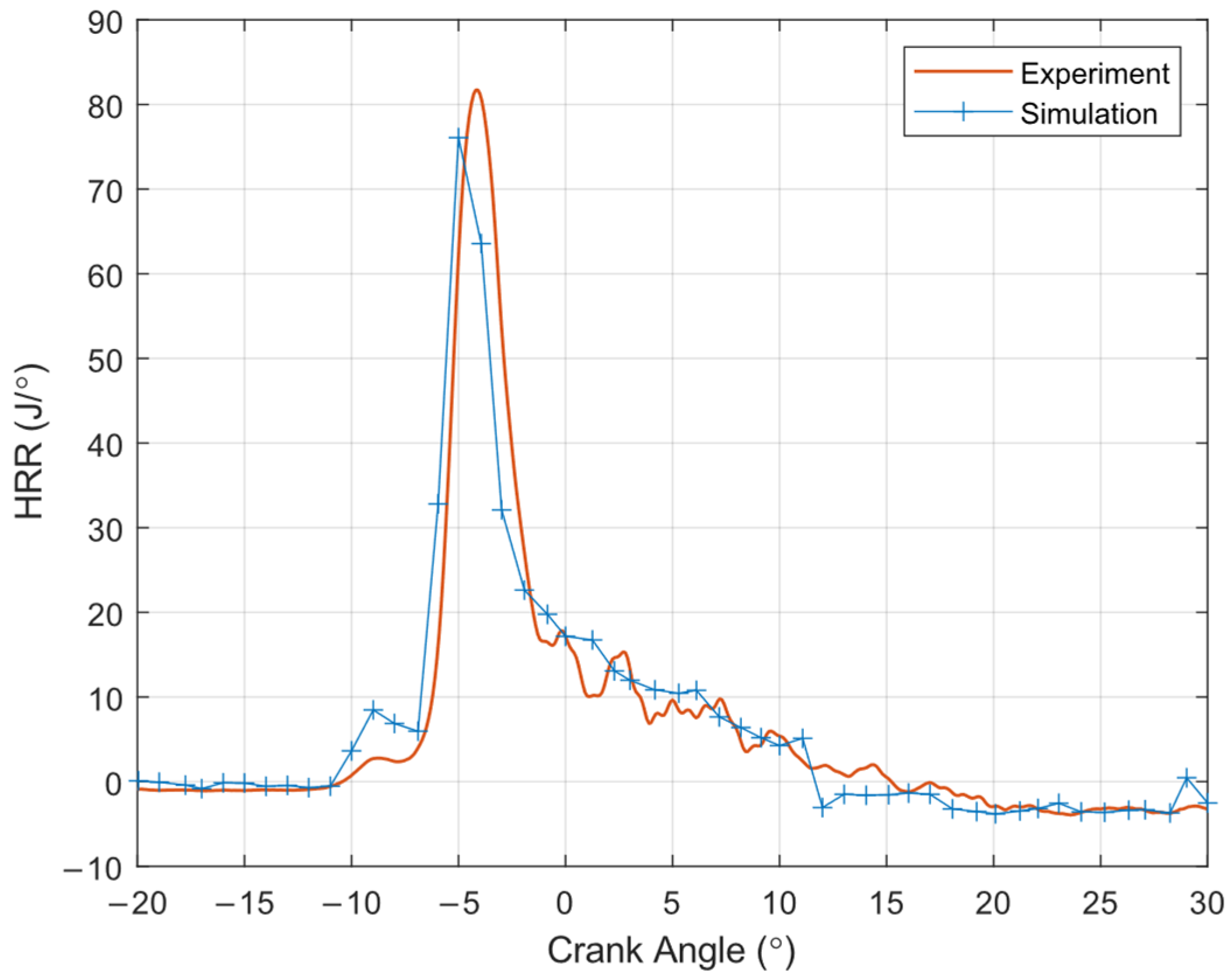
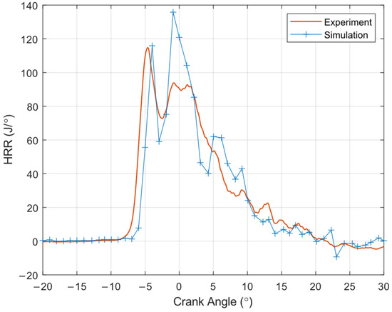
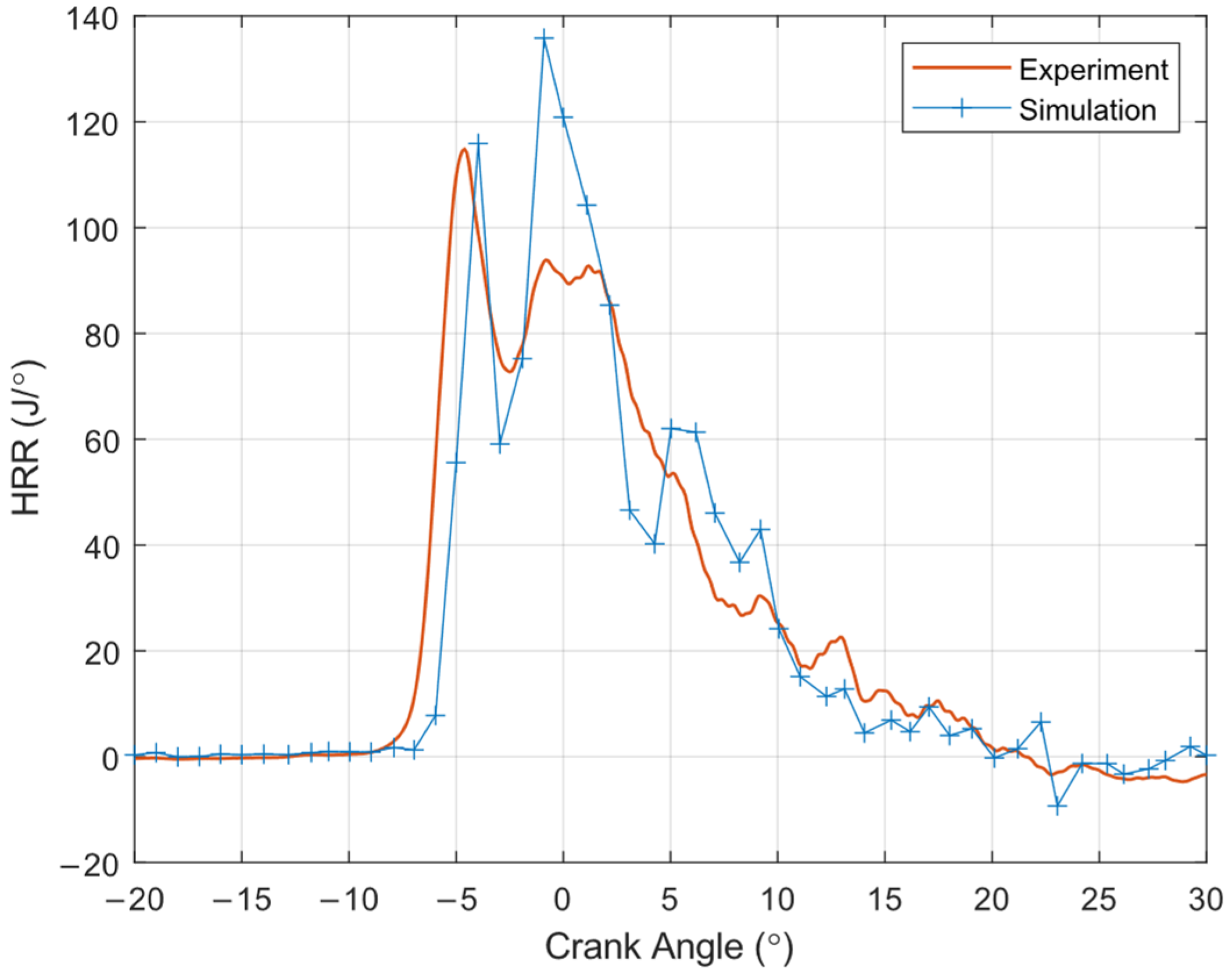
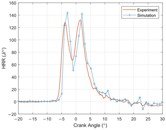
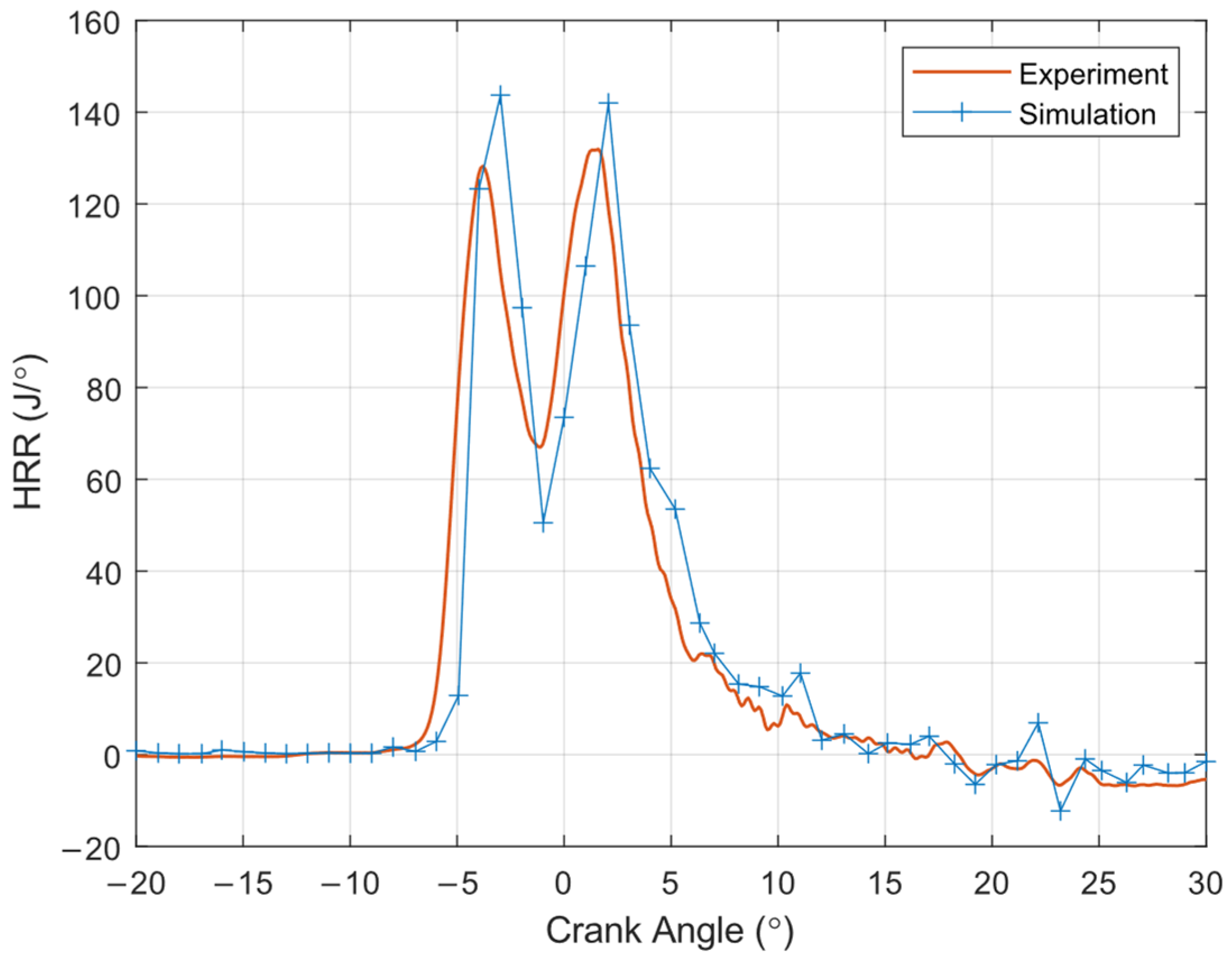
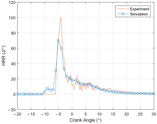
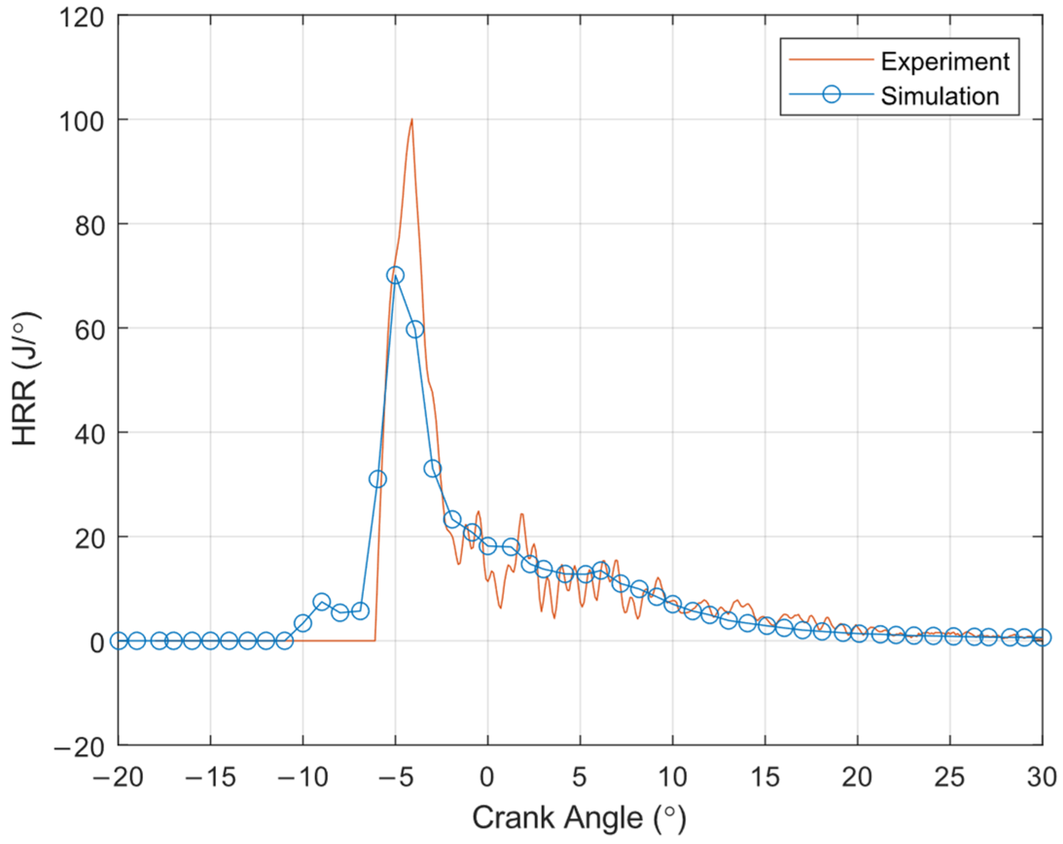
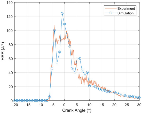
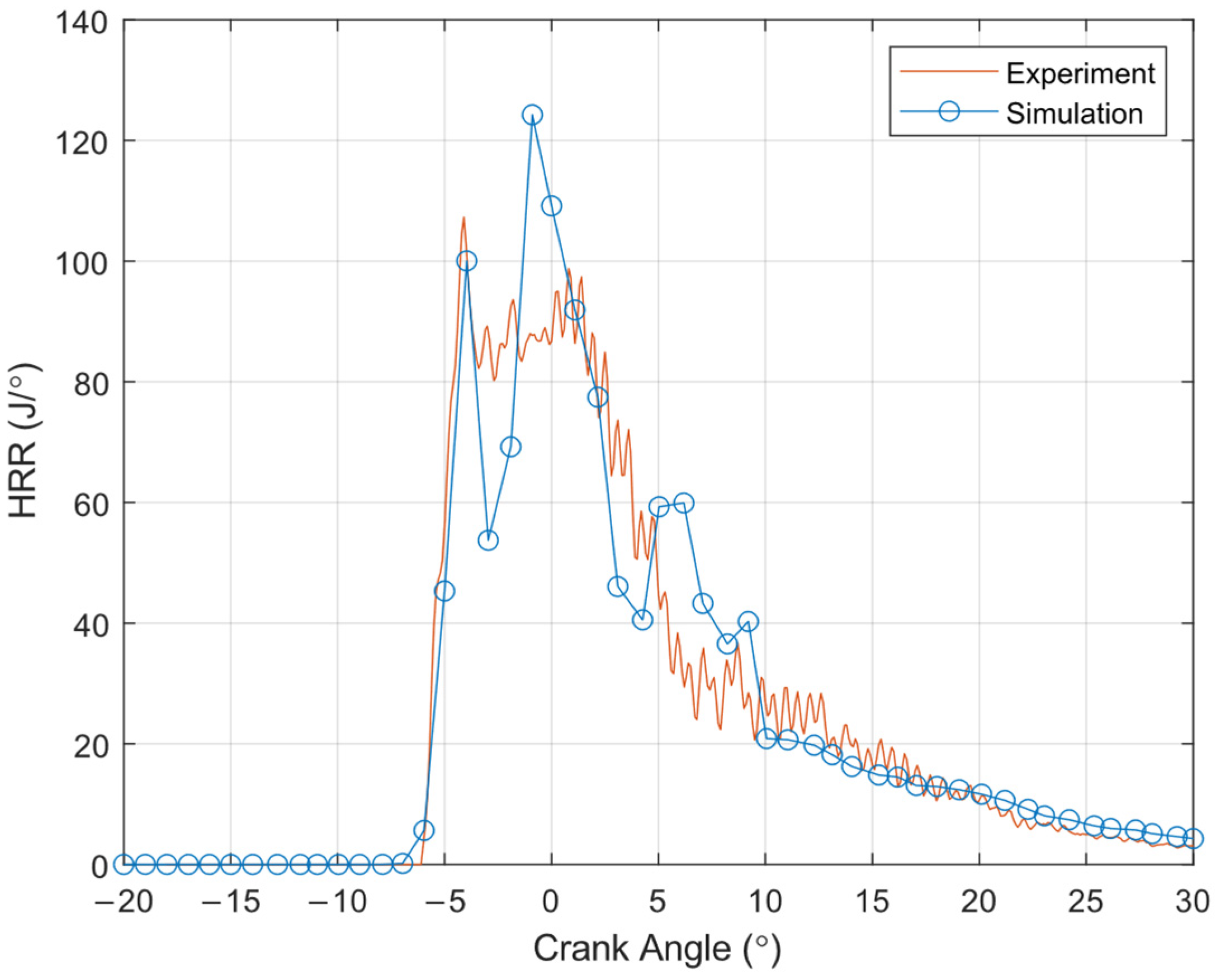
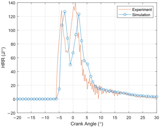
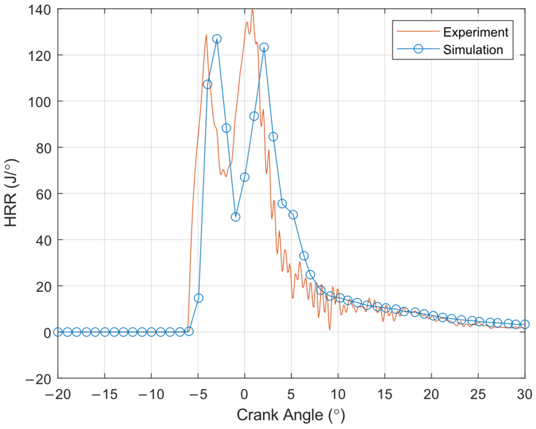
To further demonstrate the agreement between experimental and simulation results, the experiment and simulation HRR results are presented. Figure 12, Figure 13 and Figure 14 show the HRR for DO, DF-methane and DF-propane respectively using constant gamma (value of $\gamma =1.35$) Equation (1). Figure 15, Figure 16 and Figure 17 similarly show the HRR for DO, DF-methane and DF-propane but with variable gamma Equation (2). The agreement in the location and magnitude of the HRR is noted. A comparison of the HRR profiles reveals distinct characteristics between the DO and DF modes of combustion. The DO HRR curve exhibits a single prominent peak, characteristic of the premixed combustion phase in conventional diesel compression-ignition. The DF HRR profile displays an initial peak corresponding to the autoignition of the diesel pilot, followed by a second peak (particularly pronounced in the DF-propane case) due to the flame propagation through the premixed air-gaseous fuel mixture.

Figure 12. DO mode HRR from experiment and simulation using constant gamma Equation (1).

Figure 13. DF-methane mode HRR from experiment and simulation using constant gamma Equation (1).

Figure 14. DF-propane mode HRR from experiment and simulation using constant gamma Equation (1).

Figure 15. DO mode HRR from experiment and simulation using variable gamma Equation (2).

Figure 16. DF-methane mode HRR from experiment and simulation using variable gamma Equation (2).

Figure 17. DF-propane mode HRR from experiment and simulation using variable gamma Equation (2).

As discussed in the context of Figure 8, Figure 9 and Figure 10, the experimental AHR derived using the Rassweiler & Withrow method was compared with the simulation result. The experimental HRR was also obtained from the derivative of the experimental Rassweiler & Withrow AHR and is presented superimposed on the Forte chemical HRR as shown in Figure 18, Figure 19 and Figure 20. The plots show excellent agreement between experimental and simulation HRR, successfully reproducing the peak magnitudes and overall combustion phasing. Furthermore, the combustion model effectively captures the two-stage heat release (double peak) characteristic of the dual-fuel combustion process.

Figure 18. DO mode HRR from experiment using Rassweiler & Withrow AHR (EOC = 44°, PDB = 0.98) and simulation chemical HRR.

Figure 19. DF-methane mode HRR from experiment using Rassweiler & Withrow AHR (EOC = 110°, PDB = 0.98, PGB = 0.65) and simulation chemical HRR.

Figure 20. DF-propane mode HRR from experiment using Rassweiler & Withrow AHR (EOC = 120°, PDB = 0.98, PGB = 0.67) and simulation chemical HRR.

7. Conclusions

The agreement between the combustion simulation results and experimental data of in-cylinder pressure and heat release was shown. The maximum values of the chemical heat release from the simulations were above the value that would result from the multiplication of the mass of fuel and LHV. This would lead to a combustion efficiency higher than 100% which is not realistic. However, the maximum value of the chemical heat release from the simulations is just lower than the value that would result from the multiplication of mass of fuel and HHV, resulting in a realistic combustion efficiency, which on the discussion of the DO case was 97%. Therefore, it was concluded that the HHV should be used for a quantification of the AHR and HRR and not the LHV. This notion is also backed by the fact that combustion cannot foresee the end point of the expansion process and whether or not the water vapour would be able to condense. During combustion, the fuel releases its total chemical energy, corresponding to the HHV. However, whether the latent heat component can be recovered depends on the extent of the expansion process.

Appendix A.1. For Constant Gamma

Assumptions:

• The mixture contents obey the ideal gas law
• Thermodynamic properties are spatially uniform and vary only with time
• Fuel is instantaneously and completely vaporized and mixed with the air
• Blow-by is neglected

From First Law of Thermodynamics

$$Q+W=dU$$

$${\displaystyle \frac{dQ}{dt}}-p{\displaystyle \frac{dV}{dt}}={\displaystyle \frac{dU}{dt}}$$

where the term ${\displaystyle \frac{dU}{dt}}$ is the rate of change in sensible internal energy $U$; $p{\displaystyle \frac{dV}{dt}}$ is the rate of work done by the system due to boundary displacement; ${\displaystyle \frac{dQ}{dt}}$ is the rate of heat supply.

As applied for engine analysis, the rate of heat supply is referred to as the net heat release rate (apparent heat release rate) ${\displaystyle \frac{d{Q}_{net}}{dt}}$

$${\displaystyle \frac{d{Q}_{net}}{dt}}={\displaystyle \frac{d{Q}_{chem}}{dt}}-{\displaystyle \frac{d{Q}_{ht}}{dt}}=p{\displaystyle \frac{dV}{dt}}+{\displaystyle \frac{dU}{dt}}$$

where $Q_{net}$ is the difference between the chemical heat released by combustion $Q_{chem}$ and the wall heat transfer $Q_{ht}$. This form neglects the sensible enthalpy of the injected fuel $m_f{h}_f.$

$${\displaystyle \frac{d{Q}_{net}}{dt}}=p{\displaystyle \frac{dV}{dt}}+m{c}_v{\displaystyle \frac{dT}{dt}}\hspace{1em} sinceU=m{c}_{v}T$$

But

$$pV=mRT \Rightarrow pdV+Vdp=mRdT$$

(A1)

And

$$mR=pV/T$$

Dividing Equation (A1) by $mR$ or $pV/T$ on both sides

$${\displaystyle \frac{Tp}{pV}}dV+{\displaystyle \frac{TV}{pV}}dp={\displaystyle \frac{mR}{mR}}dT$$

$${\displaystyle \frac{T}{V}}dV+{\displaystyle \frac{T}{p}}dp=dT$$

Divide by T

$${\displaystyle \frac{dV}{V}}+{\displaystyle \frac{dp}{p}}={\displaystyle \frac{dT}{T}}$$

therefore

$$\begin{array}{cc}\hfill {\displaystyle \frac{d{Q}_{net}}{dt}}& =p{\displaystyle \frac{dV}{dt}}+m{c}_v{\displaystyle \frac{T}{dt}}\left({\displaystyle \frac{dV}{V}}+{\displaystyle \frac{dp}{p}}\right)\hfill \\ & =p{\displaystyle \frac{dV}{dt}}+{\displaystyle \frac{m{c}_{v}T}{V}}{\displaystyle \frac{dV}{dt}}+{\displaystyle \frac{m{c}_{v}T}{p}}{\displaystyle \frac{dp}{dt}}\hfill \\ & =\left(p+{\displaystyle \frac{m{c}_{v}T}{V}}\right){\displaystyle \frac{dV}{dt}}+{\displaystyle \frac{m{c}_{v}T}{p}}{\displaystyle \frac{dp}{dt}}\hfill \\ & =\left(p+{\displaystyle \frac{m{c}_v}{V}}{\displaystyle \frac{pV}{mR}}\right){\displaystyle \frac{dV}{dt}}+{\displaystyle \frac{m{c}_v}{p}}{\displaystyle \frac{pV}{mR}}{\displaystyle \frac{dp}{dt}}\hfill \\ & =\left(p+{\displaystyle \frac{c_{v}p}{R}}\right){\displaystyle \frac{dV}{dt}}+{\displaystyle \frac{c_{v}V}{R}}{\displaystyle \frac{dp}{dt}}\hfill \\ & =p\left(1+{\displaystyle \frac{c_v}{R}}\right){\displaystyle \frac{dV}{dt}}+{\displaystyle \frac{c_{v}V}{R}}{\displaystyle \frac{dp}{dt}}\hfill \end{array}$$

But $c_p-c_v=R$ and $\gamma =c_p/c_v$

$$\Rightarrow {\displaystyle \frac{c_v}{R}}={\displaystyle \frac{c_v}{c_p-c_v}}\Rightarrow {\displaystyle \frac{R}{c_v}}={\displaystyle \frac{c_p}{c_v}}-1=\gamma -1$$

$$1+{\displaystyle \frac{c_v}{R}}=1+{\displaystyle \frac{1}{\gamma -1}}={\displaystyle \frac{\gamma }{\gamma -1}}$$

Therefore

$${\displaystyle \frac{d{Q}_{net}}{dt}}={\displaystyle \frac{\gamma }{\gamma -1}}p{\displaystyle \frac{dV}{dt}}+{\displaystyle \frac{1}{\gamma -1}}V{\displaystyle \frac{dP}{dt}}$$

Or, for constant rotational speed

$${\displaystyle \frac{d{Q}_{net}}{d\theta }}={\displaystyle \frac{\gamma }{\gamma -1}}p{\displaystyle \frac{dV}{d\theta }}+{\displaystyle \frac{1}{\gamma -1}}V{\displaystyle \frac{dP}{d\theta }}$$

Appendix A.2. For Varying Gamma

From first law of thermodynamics

$$Q+W=dU\Rightarrow Q-pdV=dU=d\left(m{c}_{v}T\right)=m{c}_{v}dT+mTd{c}_v$$

$${\displaystyle \frac{d\mathrm{Q}}{dt}}=p{\displaystyle \frac{dV}{dt}}+m{c}_v{\displaystyle \frac{dT}{dt}}+mT{\displaystyle \frac{d{c}_v}{dt}}$$

But

$$pV=mRT\Rightarrow pdV+Vdp=mRdT+mTdR$$

(A2)

Dividing Equation (A2) by $mR$ or $pV/T$ on both sides

$${\displaystyle \frac{Tp}{pV}}dV+{\displaystyle \frac{TV}{pV}}dp={\displaystyle \frac{mR}{mR}}dT+{\displaystyle \frac{mT}{mR}}dR$$

$${\displaystyle \frac{T}{V}}dV+{\displaystyle \frac{T}{p}}dp=dT+{\displaystyle \frac{T}{R}}dR$$

Divide by T

$${\displaystyle \frac{dV}{V}}+{\displaystyle \frac{dp}{p}}={\displaystyle \frac{dT}{T}}+{\displaystyle \frac{dR}{R}}$$

$$dT=T\left({\displaystyle \frac{dV}{V}}+{\displaystyle \frac{dp}{p}}-{\displaystyle \frac{dR}{R}}\right)$$

Therefore

$${\displaystyle \frac{d{Q}_{net}}{dt}}=p{\displaystyle \frac{dV}{dt}}+m{c}_v{\displaystyle \frac{T}{dt}}\left({\displaystyle \frac{dV}{V}}+{\displaystyle \frac{dp}{p}}-{\displaystyle \frac{dR}{R}}\right)+mT{\displaystyle \frac{d{c}_v}{dt}}$$

Using $T=pV/mR$ to remove $T$

$$\begin{array}{cc}\hfill {\displaystyle \frac{d{Q}_{net}}{dt}}& =p{\displaystyle \frac{dV}{dt}}+{\displaystyle \frac{m{c}_{v}pV}{mR}}{\displaystyle \frac{1}{dt}}\left({\displaystyle \frac{dV}{V}}+{\displaystyle \frac{dp}{p}}-{\displaystyle \frac{dR}{R}}\right)+{\displaystyle \frac{mpV}{mR}}{\displaystyle \frac{d{c}_v}{dt}}\hfill \\ & =p{\displaystyle \frac{dV}{dt}}+{\displaystyle \frac{c_{v}pV}{R}}{\displaystyle \frac{1}{dt}}\left({\displaystyle \frac{dV}{V}}+{\displaystyle \frac{dp}{p}}-{\displaystyle \frac{dR}{R}}\right)+{\displaystyle \frac{pV}{R}}{\displaystyle \frac{d{c}_v}{dt}}\hfill \\ & =\left(p+{\displaystyle \frac{c_{v}p}{R}}\right){\displaystyle \frac{dV}{dt}}+{\displaystyle \frac{c_{v}V}{R}}{\displaystyle \frac{dp}{dt}}+{\displaystyle \frac{pV}{R}}{\displaystyle \frac{d{c}_v}{dt}}-{\displaystyle \frac{c_{v}pV}{R^2}}{\displaystyle \frac{dR}{dt}}\hfill \\ & =p\left(1+{\displaystyle \frac{c_v}{R}}\right){\displaystyle \frac{dV}{dt}}+{\displaystyle \frac{c_{v}V}{R}}{\displaystyle \frac{dp}{dt}}+{\displaystyle \frac{pV}{R}}{\displaystyle \frac{d{c}_v}{dt}}-{\displaystyle \frac{c_{v}pV}{R^2}}{\displaystyle \frac{dR}{dt}}\hfill \\ & =p\left(1+{\displaystyle \frac{1}{\gamma -1}}\right){\displaystyle \frac{dV}{dt}}+V{\displaystyle \frac{1}{\gamma -1}}{\displaystyle \frac{dp}{dt}}+{\displaystyle \frac{pV}{R}}{\displaystyle \frac{d{c}_v}{dt}}-{\displaystyle \frac{c_{v}pV}{R^2}}{\displaystyle \frac{dR}{dt}}\hfill \\ & =p\left({\displaystyle \frac{\gamma }{\gamma -1}}\right){\displaystyle \frac{dV}{dt}}+{\displaystyle \frac{V}{\gamma -1}}{\displaystyle \frac{dp}{dt}}+{\displaystyle \frac{pV}{R}}{\displaystyle \frac{1}{dt}}\left(d{c}_v-{\displaystyle \frac{c_v}{R}}dR\right)\hfill \end{array}$$

Considering the “3rd term”

$${\displaystyle \frac{pV}{R}}{\displaystyle \frac{1}{dt}}\left(d{c}_v-{\displaystyle \frac{c_v}{R}}dR\right)$$

Need to remove $d{c}_v$ and $dR$ to get $d\gamma$, hence use relation between $c_v$, $R$ and $\gamma$ i.e., 

$${\displaystyle \frac{R}{c_v}}=\gamma -1$$

$$R=c_v\left(\gamma -1\right)$$

$$dR=c_{v}d\gamma +\left(\gamma -1\right)d{c}_v$$

$${\displaystyle \frac{dR}{\left(\gamma -1\right)}}={\displaystyle \frac{c_v}{\left(\gamma -1\right)}}d\gamma +d{c}_v$$

$$d{c}_v-{\displaystyle \frac{dR}{\left(\gamma -1\right)}}={\displaystyle \frac{-c_v}{\left(\gamma -1\right)}}d\gamma$$

“3rd” term

$$\begin{array}{c}{\displaystyle \frac{pV}{Rdt}}\left(d{c}_v-{\displaystyle \frac{c_v}{R}}dR\right)={\displaystyle \frac{pV}{R}}{\displaystyle \frac{1}{dt}}\left(d{c}_v-{\displaystyle \frac{1}{\gamma -1}}dR\right)={\displaystyle \frac{pV}{R}}{\displaystyle \frac{1}{dt}}\left({\displaystyle \frac{-c_v}{\gamma -1}}\right)d\gamma \\ ={\displaystyle \frac{-pV}{\gamma -1}}\left({\displaystyle \frac{c_v}{R}}\right){\displaystyle \frac{d\gamma }{dt}}={\displaystyle \frac{-pV}{\gamma -1}}\left({\displaystyle \frac{1}{\gamma -1}}\right){\displaystyle \frac{d\gamma }{dt}}={\displaystyle \frac{-pV}{{\left(\gamma -1\right)}^2}}{\displaystyle \frac{d\gamma }{dt}}\end{array}$$

Therefore

$${\displaystyle \frac{d{Q}_{net}}{dt}}={\displaystyle \frac{\gamma }{\gamma -1}}p{\displaystyle \frac{dV}{dt}}+{\displaystyle \frac{1}{\gamma -1}}V{\displaystyle \frac{dP}{dt}}-{\displaystyle \frac{1}{{\left(\gamma -1\right)}^2}}pV·{\displaystyle \frac{d\gamma }{dt}}$$

Or, for constant rotational speed

$${\displaystyle \frac{d{Q}_{net}}{d\theta }}={\displaystyle \frac{\gamma }{\gamma -1}}p{\displaystyle \frac{dV}{d\theta }}+{\displaystyle \frac{1}{\gamma -1}}V{\displaystyle \frac{dP}{d\theta }}-{\displaystyle \frac{1}{{\left(\gamma -1\right)}^2}}pV·{\displaystyle \frac{d\gamma }{d\theta }}$$

References

- Rassweiler, G.M.; Withrow, L. Motion Pictures of Engine Flames Correlated with Pressure Cards. SAE Trans. 1938, 33, 185–204. [Google Scholar]
- Obert, E. Internal Combustion Engines, 3rd ed.; International Textbook Company: Scranton, PA, USA, 1968. [Google Scholar]
- Amann, C. Cylinder-Pressure Measurement and Its Use in Engine Research; SAE Technical Paper 852067; SAE International: Warrendale, PA, USA, 1985. [Google Scholar] [CrossRef] [Scilit]
- Krieger, R.B.; Borman, G.L. The computation of apparent heat release for internal combustion engines. In Proceedings of the Diesel Gas Power Conference, 2nd ed.; ASME paper 66-WA/DGP-4; American Society of Mechanical Engineers: New York, NY, USA, 1966. [Google Scholar]
- Krieger, R.B. The Simulation of a Two Cycle, Crankcase Scavenged, Spark Ignition Engine on a Digital Computer and Comparison of Results with Experimental Data. Ph.D. Thesis, University of Wisconsin Madison, Madison, WI, USA, 1968. [Google Scholar]
- Borman, G.L. Mathematical Simulation of Internal Combustion Engine Processes and Performance Including Comparisons with Experiment. Ph.D. Thesis, University of Wisconsin Madison, Madison, WI, USA, 1964. [Google Scholar]
- Heywood, J.B. Internal Combustion Engine Fundamentals; McGraw Hill Inc.: New York, NY, USA, 1988. [Google Scholar]
- Gatowski, J.A.; Balles, E.N.; Chun, K.M.; Nelson, F.E.; Ekchian, J.A.; Heywood, J.B. Heat release analysis of engine pressure data. In Proceedings of the Fuels and Lubricants Metting & Exposition, Baltimore, MD, USA, 8–11 October 1984; SAE paper 841359; SAE International: Warrendale, PA, USA, 1984. [Google Scholar] [CrossRef] [Scilit]
- Shudo, T.; Nakajima, Y.; Futakuchi, T. Thermal efficiency analysis in a hydrogen premixed combustion engine. JSAE Rev. 2000, 21, 177–182. [Google Scholar] [CrossRef] [Scilit]
- Shudo, T.; Nabetani, S.; Nakajima, Y. Influence of specific heats on indicator diagram analysis in a hydrogen-fuelled SI engine. JSAE Rev. 2001, 22, 224–226. [Google Scholar] [CrossRef] [Scilit]
- Shudo, T.; Suzuki, H. Applicability of heat transfer equations to hydrogen combustion. JSAE Rev. 2002, 23, 303–308. [Google Scholar] [CrossRef] [Scilit]
- Shudo, T. Improving thermal efficiency by reducing cooling losses in hydrogen combustion engines. Int. J. Hydrogen Energy 2007, 32, 4285–4293. [Google Scholar] [CrossRef] [Scilit]
- Ansys Forte User’s Guide, 2025 Ansys, Inc. Southpointe January 2025, 2600 Ansys Drive, Canonsburg, PA 15317, ansysinfo@ansys.com, ANSYS Europe. pg 142 “Apparent Heat Release from PV-VarGamma”. Available online: https://ansyshelp.ansys.com/public/Views/Secured/corp/v251/en/pdf/Ansys_Forte_Users_Guide.pdf (accessed on 2 February 2026).
- Lanzafame, R.; Messina, M. ICE gross heat release strongly influenced by specific heat ratio values. Int. J. Automot. Technol. 2003, 4, 125–133. [Google Scholar]
- Shayler, P.J.; May, S.A.; Ma, T. Heat Transfer to the Combustion Chamber Walls in Spark Ignition Engines; SAE Technical Paper 950686; SAE International: Warrendale, PA, USA, 1995. [Google Scholar] [CrossRef] [Scilit]
- Shayler, P.J.; May, S.A.; Ma, T. The Determination of Heat Transfer from the Combustion Chambers of SI Engines; SAE Technical Paper 931131; SAE International: Warrendale, PA, USA, 1993. [Google Scholar] [CrossRef] [Scilit]
- Wendland, D.W. The Effect of Periodic Pressure and Temperature Fluctuations on Unsteady Heat Transfer in a Closed System; National Aeronautics and Space Administration; NASA CR-72323; University of Wisconsin: Madison, WI, USA, 1968. [Google Scholar]
- Lawton, B. Effect of Compression and Expansion on Instantaneous Heat Transfer in Reciprocating Internal Combustion Engines. Proc. Inst. Mech. Eng. Part A J. Power Energy 1987, 201, 175–186. [Google Scholar] [CrossRef] [Scilit]
- Pfriem, H. Periodic Heat Transfer at Small Pressure Fluctuations. National Advisory Committee for Aeronautics, Technical Memorandum No. 1048. Page 9. Available online: https://digital.library.unt.edu/ark:/67531/metadc64740/m2/1/high_res_d/20050030010.pdf (accessed on 2 February 2026).
- Alkidas, A.C.; Myers, J.P. Transient Heat-Flux Measurements in the Combustion Chamber of a Spark-Ignition Engine. ASME J. Heat Transf. 1982, 104, 62–67. [Google Scholar] [CrossRef] [Scilit]
- Chun, K.M.; Heywood, J.B. Estimating Heat-Release and Mass-of-Mixture Burned from Spark-Ignition Engine Pressure Data. Combust. Sci. Technol. 1987, 54, 133–143. [Google Scholar] [CrossRef] [Scilit]
- Wang, B.; Lin, H.; Bai, C.; Yang, C.; Chen, Y.; Zu, Z.; Yin, Y.; Cheng, X.; Li, Z. Combustion and heat transfer characteristics of a heavy-duty low-pressure-direct-injection hydrogen engine with a flat-roof-and-shallow-bowl combustion chamber. Int. J. Hydrogen Energy 2024, 96, 597–611. [Google Scholar] [CrossRef] [Scilit]
- Beccari, S.; Pipitone, E.; Caltabellotta, S. Analysis of the Combustion Process in a Hydrogen-Fueled CFR Engine. Energies 2023, 16, 2351. [Google Scholar] [CrossRef] [Scilit]
- Beccari, S.; Pipitone, E. Heat Transfer Modeling of Hydrogen-Fueled Spark Ignition Engine. Energies 2025, 18, 475. [Google Scholar] [CrossRef] [Scilit]
- Pukalskas, S.; Rimkus, A.; Vipartas, T.; Stravinskas, S.; Kriaučiūnas, D.; Mejeras, G.; Ušinskas, A. Hydrogen Supplementation in SI Engines: Enhancing Efficiency and Reducing Emissions with a Focus on Knock Phenomena. Machines 2025, 13, 571. [Google Scholar] [CrossRef] [Scilit]
- Shao, K.; Wu, H. Effect of Hydrogen Injection Strategy on Combustion and Emissions of Ammonia–Hydrogen Sustainable Engines. Sustainability 2025, 17, 9403. [Google Scholar] [CrossRef] [Scilit]
- Willems, R.; Seykens, X.; Bekdemir, C.; Doosje, E.; Van Gompel, P. The Potential of Hydrogen High Pressure Direct Injection Toward Future Emissions Compliance: Optimizing Engine-Out NOx and Thermal Efficiency; SAE Technical Paper 2024-37-0005; SAE International: Warrendale, PA, USA, 2024. [Google Scholar] [CrossRef] [Scilit]
- Karim, G.A. Dual-Fuel Diesel Engines; CRC Press: London, UK, 2021. [Google Scholar]
- Weaver, C.S.; Turnier, S.H. Dual Fuel Natural Gas/Diesel Engines: Technology, Performance, and Emissions. In Proceedings of the International Congress and Exposition, Detroit, MI, USA, 28 February–3 March 1994; pp. 77–92; SAE Technical Paper 940548; SAE International: Warrendale, PA, USA, 1994; pp. 77–92. [Google Scholar]
- Ricardo, H.R. Recent research work on the internal combustion engine. SAE Trans. 1922, 17, 1–93. [Google Scholar]
- Saliba, A.T.; Agius, E.; Scerri, K.; Farrugia, M. Simulation of operation and control of LNG and diesel dual fuel engine for marine application. In Proceedings of the 7th Offshore Energy & Storage Symposium (OSES 2023), St. Julian’s, Malta, 12–14 July 2023; Volume 2023, pp. 349–356. [Google Scholar] [CrossRef] [Scilit]
- Mifsud, S.; Azzopardi, J.P.; Farrugia, M. Liquefied Petroleum Gas (LPG) and Diesel, Dual Fuel Implementation on a Common Rail Diesel Engine. In Proceedings of the 2020 19th International Conference on Mechatronics-Mechatronika (ME), Prague, Czech Republic, 2–4 December 2020; IEEE: Piscataway, NJ, USA, 2020; pp. 192–199. [Google Scholar] [CrossRef] [Scilit]
- Pipitone, E.; Beccari, A. Determination of TDC in internal combustion engines by a newly developed thermodynamic approach. Appl. Therm. Eng. 2010, 30, 1914–1926. [Google Scholar] [CrossRef] [Scilit]
- Saliba, A.T.; Xiang, L.; Mollicone, J.P.; Ding, Y.; Farrugia, M. Dual Fuel Combustion Modelling Using the G-Equation Model and the Respective tuning of Flame Stretch Parameters. Energies 2026, 19, 1021. [Google Scholar] [CrossRef] [Scilit]
- Rahimi, A.; Fatehifar, E.; Saray, R.K. Development of an optimized chemical kinetic mechanism for homogeneous charge compression ignition combustion of a fuel blend of n-heptane and natural gas using a genetic algorithm. Proc. Inst. Mech. Eng. Part D J. Automob. Eng. 2010, 224, 1141–1159. [Google Scholar] [CrossRef] [Scilit]
- Ansys. ANSYS Model Fuel Library Getting Started Guide—2023 R1; Ansys: Canonsburg, PA, USA, 2023. [Google Scholar]
- Amsden, A.A. Improved Law-of-the-Wall Heat Transfer Model. In KIVA-3V: A Block-Structured KIVA Program for Engines with Vertical or Canted Valves; LA-13313-MS, UC-1412; Los Alamos National Laboratory: Los Alamos, NM, USA, 1997. Available online: https://digital.library.unt.edu/ark:/67531/metadc693255/m2/1/high_res_d/505339.pdf (accessed on 2 February 2026).
- Olanrewaju, F.O.; Wu, Y.; Li, H.; Andrews, G.; Phylaktou, H. An Improved Heat Release Rate (HRR) Model for the Analysis of Combustion Behaviour of Diesel, GTL, and HVO Diesel. In Proceedings of the SAE Powertrains, Fuels & Lubricants Meeting, Online, 22–23 September 2020; SAE Technical Paper Series; SAE International: Warrendale, PA, USA, 2020; Article no: 2020-01-2060. [Google Scholar] [CrossRef] [Scilit]
- Portelli, S.; Farrugia, M. Mechatronics for Hydrogen Fuelling of Single Cylinder Internal Combustion Engine. In Proceedings of the 20th International Conference on Mechatronics—Mechatronika (ME), Pilsen, Czech Republic, 2022; IEEE: Piscataway, NJ, USA, 2022; pp. 1–7. [Google Scholar] [CrossRef] [Scilit]
- Saliba, A.T.; Schembri, M.; Scerri, K.; Farrugia, M. Implementation of Electronic Throttle for Control of a Dual Fuel Diesel Engine. In Proceedings of the 7th International Conference on Control, Automation and Diagnosis ICCAD2023, Rome, Italy, 10–12 May 2023; IEEE: Piscataway, NJ, USA, 2023. [Google Scholar]
Disclaimer/Publisher’s Note: The statements, opinions and data contained in all publications are solely those of the individual author(s) and contributor(s) and not of MDPI and/or the editor(s). MDPI and/or the editor(s) disclaim responsibility for any injury to people or property resulting from any ideas, methods, instructions or products referred to in the content. |
© 2026 by the authors. Licensee MDPI, Basel, Switzerland. This article is an open access article distributed under the terms and conditions of the Creative Commons Attribution (CC BY) license.