Article

A Hybrid Decision Framework for Greenness Evaluation of Offshore Oil and Gas Field Extraction

1
College of Publishing, University of Shanghai for Science and Technology, Shanghai 200093, China
2
Business School, University of Shanghai for Science and Technology, Shanghai 200093, China
*
Author to whom correspondence should be addressed.
Energies 2026, 19(6), 1398; https://doi.org/10.3390/en19061398
Submission received: 15 January 2026 / Revised: 28 February 2026 / Accepted: 6 March 2026 / Published: 10 March 2026

Abstract

Under the global trend of low-carbon transition, the sustainability and greenness of offshore oil and gas field (OOGF) extraction projects can no longer be ignored. Existing studies rarely evaluate the greenness of OOGF extraction projects, so this paper proposes a hybrid decision-making framework for the green plants of OOGF extraction projects. First, a comprehensive evaluation criteria system for offshore oil and gas field green plants (OOGFGPs) is innovatively constructed, including green energy utilization, green performance, economy, society, environment and risk. In addition, for the interacting evaluation criteria and the uncertainty of decision-making information, this paper adopts a spherical fuzzy decision-making test and evaluation laboratory (SF–DEMATEL) to calculate the weights of criteria. Ultimately, SF-based multi-attribute ideal-real comparative analysis (SF–MAIRCA) is proposed to evaluate the OOGFGPs. Taking the OOGF extraction projects in the Bohai Sea of China as an example, the proposed decision-making framework is verified to have good stability and applicability through validation analysis, sensitivity analysis and comparative analysis.

1. Introduction

Offshore oil and gas production holds paramount significance in addressing the escalating global demand for energy. Since the turn of the century, offshore facilities have contributed a substantial 30% to global oil production and 27% to gas production, thus playing a pivotal role in satisfying the world’s energy requirements [1]. Conventionally, offshore oil and gas facilities have relied on gas turbines installed on platforms, powered by the combustion of natural gas [2], which is considered a wasteful and environmentally unfriendly approach. Given the urgency of global climate goals, particularly the emission reduction targets outlined in the Paris Agreement, reducing greenhouse gas emissions from high-emission industries such as offshore oil and gas extraction has become a critical step in mitigating climate change. The global demand to reduce methane emissions—as methane has a far higher greenhouse effect than carbon dioxide—has prompted nations to take urgent action [3]. In this context, the offshore oil and gas industry’s role in methane leaks and carbon dioxide emissions is increasingly under scrutiny. As countries and regions accelerate their transition to low-carbon and green energy, the environmental sustainability of offshore oil and gas fields (OOGFs) has become essential [4].
A green offshore oil and gas field extraction plant is a plant that minimizes the adverse environmental impacts of OOGF extraction in terms of production, design and operation; improves the efficiency of oil and gas resource utilization; and promotes energy decarbonization and sustainable economic development. An offshore oil and gas field green plant (OOGFGP) aims to realize a win–win situation for both production and environmental protection by adopting clean production technologies, circular economy models and energy-saving and environmental protection measures. The evaluation of OOGFGP is of great significance for implementing green manufacturing, accelerating green transformation and the development of manufacturing industry, and promoting stable growth of the industry. Therefore, more attention needs to be paid to the evaluation of OOGFGP. Evaluating the greenness of OOGFGP is not only crucial for advancing green manufacturing, but also helps align the industry with global decarbonization goals, including reductions in methane and carbon dioxide emissions.
Evaluating OOGFGP requires a combination of multiple criteria. Therefore, evaluating OOGFGP falls within the realm of research on multi-attribute decision making (MCDM) [5]. Many scholars have studied the sustainability of the OOGF industry and the offshore manufacturing industry, as shown in Table 1. By summarizing the literature, we find that studies on the sustainability of the OOGF industry mainly focus on the decommissioning of OOGF facilities, and studies on the sustainability of offshore manufacturing mainly focus on the siting of offshore wind farms. Green evaluation of OOGF extraction projects is lacking in the OOGF and offshore manufacturing industries. Therefore, considering the importance of energy sustainability and green development in OOGF extraction projects, this paper proposes a hybrid decision-making framework for evaluating the greenness of extraction projects in OOGFs. The proposed framework encompasses three distinct components: the articulation of experts’ ambiguous evaluation information, the computation of criteria weights, and the prioritization of alternatives [6].
In practical evaluation problems, there is always a certain degree of ambiguity, information incompleteness and uncertainty, and determining the important criteria and optimal programs affecting the green plants in OOGFs is no exception. In addition, experts may have different levels of science, experience, and perspectives when assessing criteria and programs affecting green plants in offshore oil and gas fields. Furthermore, experts may have incomplete data for reasons of confidentiality or their opinions may be characterized by ambiguity and uncertainty. In such cases, the use of fuzzy sets is required [20].
There are such fuzzy sets, and these include classical fuzzy sets [21], intuitionistic fuzzy numbers (INFNs) [22], Pythagorean fuzzy sets (PFS) [23], etc. Classical fuzzy sets have been criticized because their membership grades are deterministic and do not show skepticism and non-membership degrees. INFNs have grades of non-membership, membership, and skepticism, but INFNs cannot fully show uncertainty in real-life situations. The main difference between PFS and INFNs is the solution space, PFS provide decision makers (DMs) with greater degrees of freedom than INFNs [24,25]. However, unlike INFNs and PFS, in spherical fuzzy (SF) sets, the degrees of membership, non-membership, and hesitation are defined independently (with values between 0 and 1) [26]. SF sets allow the DMs to define the affiliation function within a spherical region and to assign degrees of membership independently with a larger domain available to express the DM’s preferences. Consequently, this paper utilizes SF sets to handle the uncertainty information pertaining to the evaluation of OOGFGP.
The next step is to address the problem of conflicting and interacting evaluation criteria. In multi-attribute decision making, common methods for calculating weights are the analytic hierarchy process (AHP), data envelopment analysis (DEA), grey relational analysis (GRA), etc. The AHP method constructs the hierarchical structure of the decision problem and fills in the judgment matrix based on the subjective judgment of the DM. The DEA method calculates the efficiency score through a linear programming model, which may underestimate or overestimate the influence of criteria to the evaluation results. The GRA method evaluates the importance of criteria by calculating the gray correlation, but the method requires sufficient sample data and is limited when dealing with complex decision problems. The decision evaluation and measurement by trial and error (DEMATEL) method not only determines attribute weights but also maps causal relationships among attributes, identifying the most critical ones. Consequently, it has garnered significant attention in evaluation research [27,28]. Gül [29] proposed an SF sets extension of DEMATEL. There exist many studies combining SF sets and DEMATEL methods to make decisions. Zhu et al. [30] used SF–DEMATEL to identify important maintenance items for machine tools. Büyüközkan et al. [31] utilized SF–DEMATEL to select renewable energy in Turkey. Erdoğan et al. [32] adopted SF–DEMATEL to evaluate autonomous vehicle driving systems. According to these studies, we found that SF–DEMATEL method can deal with the uncertainty of information more accurately and express the interrelationships between the criteria and assign weights. Therefore, in this paper, SF–DEMATEL is adopted to calculate the weights of criteria affecting OOGFGP.
The proposed framework’s final step is to rank the alternatives. There exist a host of MCDM methods like AHP (Analytic Hierarchy Process), TOPSIS (Technique for Order Preference by Similarity to an Ideal Solution), ELimination Et Choix Traduisant la Realitéwas (ELECTRE), etc. AHP is well-suited for scenarios that the number of criteria is limited. TOPSIS is more appropriate in cases where sufficient raw data is available for quantitative analysis. The ELECTRE method can take into account the interplay between multiple decision criteria and weights. But the ELECTRE method requires a large number of calculations and may be subjective during the decision-making process. The Multi-Attribute Ideal-Real Comparative Analysis (MAIRCA) approach, introduced by Pamucar et al. [33], exhibits greater stability compared to other MCDM techniques such as TOPSIS or ELECTRE. The MAIRCA method relies on a straightforward mathematical algorithm and can be seamlessly integrated with other methodologies, rendering it a promising approach deserving of further research and development efforts [34]. Haq et al. [35] reviewed the MAIRCA method and showed that the existing research on the MAIRCA methodology considered fuzzy environments. However, the SF set expresses the decision maker’s preferences better than other fuzzy sets, and there are few studies on the SF–MAIRCA combination. Dınçer et al. [36] firstly proposed a method combining interval-valued SF–MAIRCA with a complex decision-making process. However, few studies have been conducted on the combination of SF and MAIRCA. Therefore, SF–MAIRCA is proposed to rank alternatives in the evaluation of OOGFGP.
In this paper, a green evaluation model is innovatively proposed for the evaluation of OOGFGP to promote the sustainable development of offshore manufacturing industry and accelerate the construction of a green manufacturing and service system. In this model, we use SF–DEMATEL to determine the weights of OOGFGP criteria, and SF–MAIRCA is proposed to rank the candidate OOGF green extraction projects in China. As a result, through sensitivity analysis and comparative analysis, the proposed model is verified to have good stability and applicability. The main contributions of this work are as follows:
  • This study innovatively develops a comprehensive evaluation criteria system specifically tailored for OOGFGPs. By incorporating multiple interacting dimensions such as green energy utilization, green performance, environment, safety, and society, the system accurately captures the uniqueness of offshore extraction.
  • To address the highly interwoven nature of offshore evaluation criteria, the SF–DEMATEL method is applied to OOGFGPs for standard weighting. This application surpasses traditional weighting methods by not only directly showcasing the causal relationships between multiple criteria but also precisely expressing the DMs’ preferences and accommodating their hesitancy.
  • The SF–MAIRCA method is integrated to assess and rank the greenness of OOGF extraction projects. By calculating the gap between the theoretical ideal state and empirical realities, this method enables decision-makers to make mathematically stable and rational decisions in a highly subjective evaluation environment.
The rest of paper is structured as follows. In Section 2, we establish a comprehensive evaluation criteria system of OOGFGP. Section 3 introduces the SF-set-based decision-making framework, which integrates the DEMATEL and MAIRCA methods. In Section 4, we apply the methodology proposed in this paper to the evaluation of green factories in China’s OOGFs and verify the effectiveness of the proposed methodology through sensitivity and comparative analyses. The last part summarizes the whole paper.

2. Evaluation Criteria System of OOGFGP

Determination of the evaluation criteria system of green factories in OOGFs has a crucial role in the low-carbon transformation of OOGFs and to their development in a green manner. The existing sustainable development of OOGFs in various countries focuses mainly on the decommissioning research of OOGF facilities. Additionally, most of the research on the sustainable development of the offshore manufacturing industry is on the siting of offshore wind farms. Green evaluation of OOGF extraction projects is lacking in the OOGF industry and the offshore manufacturing industry. China’s Ministry of Industry and Information Technology (MIIT) has released the General Rules for Green Factory Evaluation (GB/T 36132-2018) [37], which provides a technical standard to be referred to for the creation and evaluation of green factories for offshore mining, and also provides a general technical framework for each industry to develop green factory evaluation standards or specific requirements [37].
In this study, OOGFGP refers to all green facilities or platforms involved in offshore oil and gas field extraction projects. Specifically, it includes all facilities and systems directly involved in reducing environmental impacts, improving resource efficiency, and promoting sustainability, such as oil and gas extraction platforms, energy production systems, and pollution control equipment. The system boundaries used in this study encompass the entire offshore oil and gas extraction process, from production and design to the operational phase. These boundaries include assessments of green energy utilization, environmental performance, energy efficiency, pollution emissions, and socio-economic impacts. Our focus is on evaluating the greenness of the entire offshore oil and gas field development project, rather than the greenness of a single facility or platform.
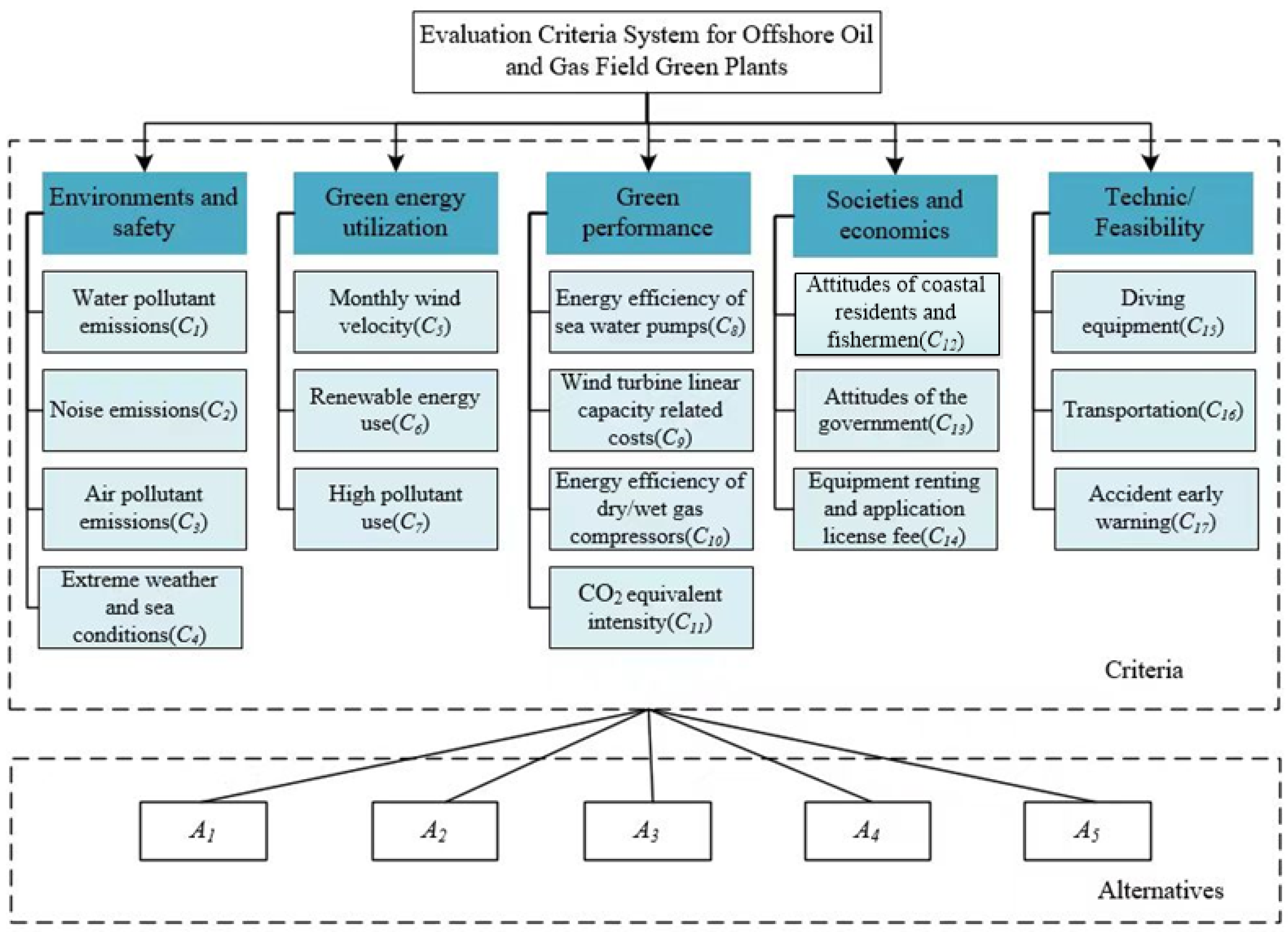
Several scholars have studied the criteria that affect the sustainable development of OOGFs. Iaiani et al. [38] analyzed the importance of security attacks on offshore oil and gas facilities and related activities, but did not consider energy, economic and environmental factors on the security of OOGF facilities. Almedallah and Walsh [39] take into account the existence of existing infrastructure and the cost of installing new surface facilities for field developments, but do not incorporate the environmental, social, and safety risks and the sustainable energy use of OOGFs into the economic impacts on field development. D’Antoine et al. [40] studied the mental health hazards of workers in the offshore oil and gas industry, but did not take into account the interplay of governmental attitudes, local residents, and other factors. Socolofsky et al. [41] analytically quantified the mass fraction of oil and gas at the surface and benzene, but did not consider the impact of other carbon dioxide equivalents and pollutant emissions on the transport to the sea surface. By analyzing the existing studies on the environmental development of OOGF projects and the GB/T 36132-2018 standard, we established a comprehensive evaluation criteria system for OOGFGP, as shown in Figure 1.

2.1. Environments and Safety

Environmental and security attacks against OOGF facilities can capitalize on the inherent hazards posed by large quantities of hazardous substances, with serious impacts on people, the environment and assets [42]. Therefore, contamination ranging from solids, liquids to gases, and the effects of extreme weather are all factors that should be considered when determining the OOGFGP.
(1)
Water pollutant emissions (C1) [43]
Offshore oil and gas extraction projects generate large quantities of wastewater. Inadequate treatment of wastewater discharges can directly lead to a decline in seawater quality, affecting the survival and reproduction of marine life.
(2)
Noise emissions (C2) [44]
Offshore oil and gas extraction projects operate at a constant level of loud decibel noise, which can adversely affect marine life as well as fishermen and residents in the vicinity.
(3)
Air pollutant emissions (C3) [45,46]
Offshore oil and gas extraction projects emit large quantities of exhaust gases containing volatile organic compounds, as well as greenhouse gases such as carbon dioxide, nitrogen oxides and acid gases. These emissions can cause air pollution and affect human health and agricultural production.
(4)
Extreme weather and sea conditions (C4) [47,48]
In the process of OOGF development, extreme weather conditions such as typhoons and tsunamis lead to high extraction costs for OOGF extraction operations, as well as safety problems for offshore operators and equipment. In addition, extreme weather can affect marine biodiversity, which also has a significant impact on local revenues.

2.2. Green Energy Utilization

Low-carbon energy efficiency in manufacturing is related to the evolution of industrialization and the construction of industrial systems with significant national differences. Low-carbon energy efficiency plays a key role in green factory performance assessment with a green trend. The specialized equipment used in factories should comply with industry access requirements, reduce energy and resource consumption, and reduce pollutant emissions.
(1)
Monthly wind velocity (C5) [49,50]
At present, Chinese offshore oilfields mainly use fossil energy to supply electricity, and wind power provides a cleaner and low-carbon new idea for deep-sea oilfields to use electricity. At the same time, the uncertainty of wind size also puts higher requirements on the stability of the oilfield group grid, so the monthly average wind speed is also used as one of the considerations for determining the OOGFGP.
(2)
Renewable energy use (C6) [51,52]
In the context of the “dual-carbon strategy”, the active development of renewable energy and the promotion of the synergistic development of offshore wind power, onshore photovoltaic and green hydrogen energy industries are very important [53]. Therefore, renewable energy use is the key to the green development of OOGF projects.
(3)
High pollutant use (C7) [54]
The augmentation of oil and gas reserves and production in OOGFs has resulted in a notable surge in carbon emission intensity. As the exploitation duration of producing OOGF elongates, the challenges associated with stabilizing oil and controlling water growth, contributing to a gradual escalation in energy consumption and a yearly increase in carbon emissions within the oilfields. Consequently, the utilization of high pollutants has a significant impact on the pursuit of low-carbon development in OOGF projects. This criterion specifically addresses the intensity of carbon emissions and the rise in pollutant use as extraction duration increases, distinct from other emissions standards that focus on specific pollutants like CO2 or VOCs.

2.3. Green Performance

The performance of green factories mainly refers to the completion of production within the specified range, the statistics of production and output value, and the calculation of relevant performance emissions. The performance of a green factory is the result, and the accounting of performance indicators depends on the organization of the company, and several performance criteria will affect the final greenness assessment of the mining project.
(1)
Energy efficiency of sea water pumps (C8) [55,56]
The energy consumption of major energy-consuming equipment, such as seawater pumps, oil transfer pumps, and gas turbines, has been increasing year by year as a percentage of oil and gas operating costs. The analysis of the energy efficiency of seawater pumps holds a pivotal role in controlling the rise of the energy consumption of offshore crude oil production, reducing the cost of crude oil production and realizing the greening of OOGF production.
(2)
Wind turbine linear capacity related costs (C9) [40,49]
Offshore wind turbines are taller and heavier than onshore wind turbines. Large wind turbines require large amounts of energy to operate, and wind farms must use electricity from the grid, which comes from coal, natural gas, or nuclear power. Although turbines can generate electricity, they are dependent on external power sources for their own proper operation. Therefore, the costs associated with the linear capacity of wind turbines can impact the operation of an OOGF project.
(3)
Energy efficiency of dry/wet gas compressors (C10) [56]
The compressor is the core equipment of offshore oil extraction, and will directly affect the economy of production and final revenue. Oil platforms are required to strengthen the analysis and research on the application effect of compressors and select the type of compressor suitable for the current working conditions, which in turn is conducive to the design of oilfield gas extraction and energy saving and emission reduction. Therefore, the energy efficiency of wet and dry gas compressors affects the sustainable development of OOGFs.
(4)
CO2 equivalent intensity (C11) [57]
CO2 equivalent serves as the unit of measurement that is essential for comparing various greenhouse gas emissions, thereby facilitating the harmonization of results pertaining to the overall greenhouse effect [58]. Offshore oil and gas fields are relatively independent and are subject to platform space constraints that make it difficult to achieve full recovery and utilization of offshore associated gas, therefore leading to the production of flaring emissions. These emissions are expressed in terms of CO2 equivalent intensity and have a significant impact on OOGF projects. C11 is specifically focused on CO2 emissions from flaring, distinguishing it from other emissions criteria that address broader atmospheric pollutants.

2.4. Societies and Economics

In OOGF sustainable development, the societies and economics of OOGFGP are critical. It is important to consider the government’s attitude as well as potential costs such as manpower and material resources when determining the OOGFGP.
(1)
Attitudes of coastal residents and fishermen (C12) [59,60]
The OOGF industry concurrently presents substantial hazards to offshore environmental pollution and biodiversity [61]. The impact of OOGF extraction on coastal residents and fishermen is complex. On the one hand, various types of pollution are not conducive to the lives of residents, while the impact on marine biodiversity may cause income problems for fishermen. Accelerating the utilization of renewable energy, forming a green mining transformation, and minimizing pollution can help to gain support from surrounding residents and fishermen [62].
(2)
Attitudes of government (C13) [61]
OOGF extraction is hugely profitable for society, providing employment for millions of people and generating significant tax revenues for governments [62,63,64]. The government needs to consider both the considerable benefits of OOGF extraction and its adverse impacts on the marine environment and biodiversity in an integrated manner.
(3)
Equipment renting and application license fee (C14) [65,66]
For oil companies, purchasing various equipment and applying for license fees require huge capital investment. However, equipment leasing can reduce the investment cost and use the money for other important aspects, such as research and development, carbon reduction, etc. Therefore, equipment leasing and license fee application have a greater impact on the green exploitation evaluation of OOGF projects.

2.5. Technic/Feasibility

In OOGF sustainable development, OOGFGP develops facilities and technical risks that determine the proper functioning of subsea operations in deep water environments. Transportation capabilities and accident warning capabilities determine the sustainability of the project in the mid and late stages of the OOGFGP development process. These factors are critical and interact with each other.
(1)
Diving equipment (C15) [9,66]
The importance of diving equipment such as underwater robots is self-evident due to the harsh environment of deep water and the limited diving depth of humans. In practical application, each drilling platform will be equipped with different levels of underwater robots according to the water depth capacity. Therefore, diving equipment has an impact on the sustainable development of OOGF projects.
(2)
Transportation (C16) [65,66]
On offshore platforms, oil is lifted from the seabed and extracted to the surface for crude processing only, with the target product being crude oil with less than 1 per cent water content, which is then transported to land terminals for further processing. The transportation process can have an impact on the surrounding environment and it is therefore important to consider transportation factors.
(3)
Accident early warning (C17) [1]
An oil drilling project is a complex engineering system, one which contains a variety of equipment and processes. Offshore oil extraction is even more complex and difficult, accidents may occur, including but not limited to wellhead collapse, oil field gas leakage, etc. These accidents, once they have occurred, will cause large losses and could even jeopardize the safety of personnel, so the application of early warning technology has become particularly important.
To present each evaluation criterion’s information more clearly, we have consolidated the information from C1 to C17 into Table 2.

3. Methodology

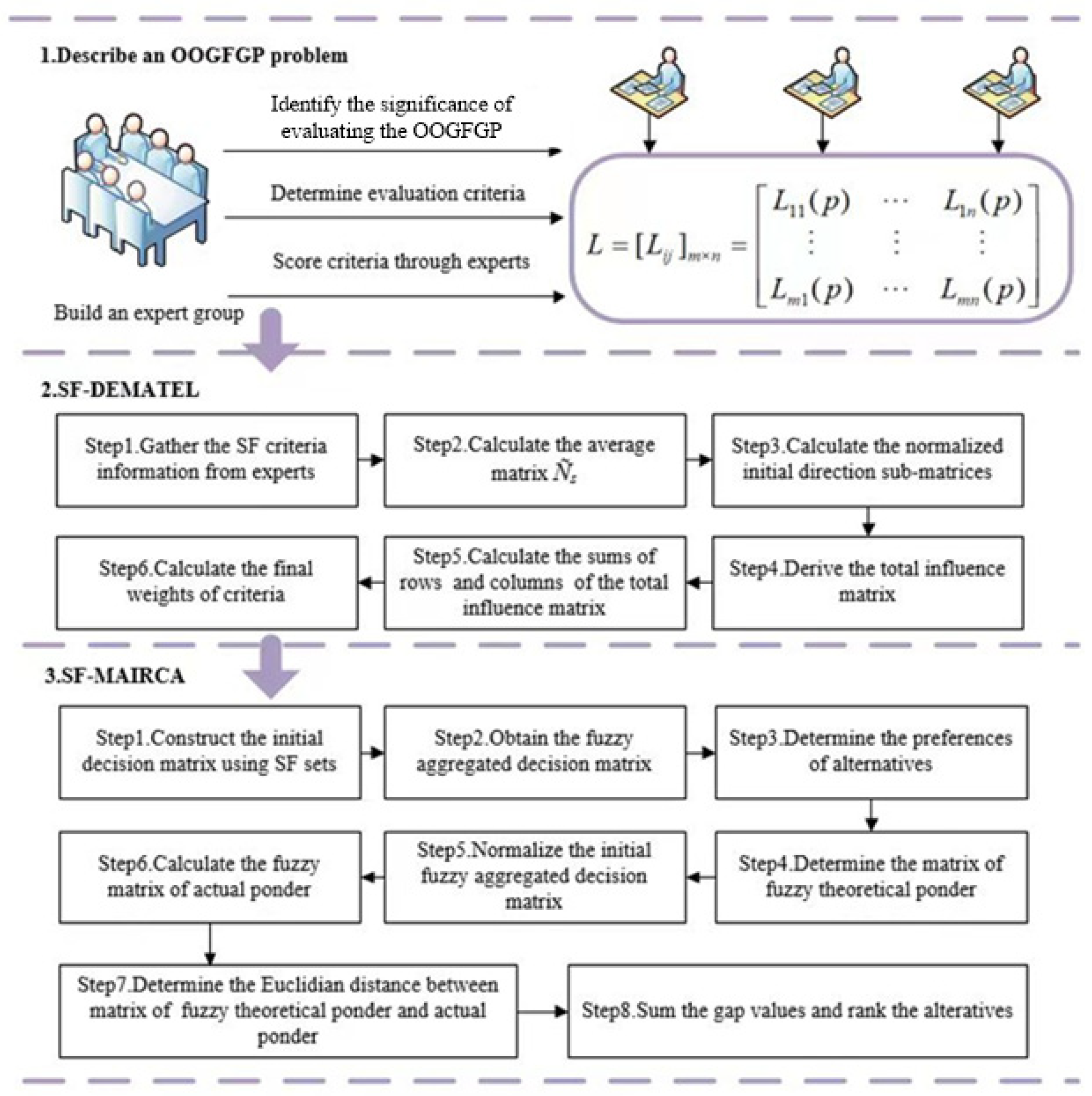
To facilitate a scientific evaluation of the OOGFGP, a comprehensive multi-attribute decision-making framework has been devised and is presented in Figure 2. In this paper, the modified DEMATEL and MAIRCA are used to solve the MCDM problem in the evaluation of OOGFGP. The specific process is described in this section.

3.1. Preliminaries of SF Sets

SF sets represent a novel extension of fuzzy sets, and are characterized by three-dimensional membership functions that enable a more nuanced linguistic assessment by experts. Definitions 1–5 outline the fundamental concepts of SF sets, while the notations and their corresponding meanings are enumerated in Table 3.
Definition 1 
([26]). Defining X as the universe of discourse, the SF set A ˜ s on X is defined as follows:
A ˜ s = x , μ A ˜ s ( x ) , ν A ˜ s ( x ) , π A ˜ s ( x ) | x X ,
where μ A ˜ s : x [ 0 , 1 ] , ν A ˜ s : x [ 0 , 1 ] , and π A ˜ s : x [ 0 , 1 ] are the degrees of membership, non-membership, and hesitancy of x to A ˜ s , and 0 μ A ˜ s 2 ( x ) + ν A ˜ s 2 ( x ) + π A ˜ s 2 ( x ) 1 . A ˜ s and x X , δ A ˜ s = 1 μ A ˜ s 2 ( x ) ν A ˜ s 2 ( x ) π A ˜ s 2 ( x ) are the degrees of refusal of x to A ˜ s .
Definition 2 
([26]).  A ˜ s 1  and  A ˜ s 2 are two SF sets with operations defined as follows:
Addition ( A ˜ s 1 A ˜ s 2 ):
A ˜ s 1 A ˜ s 2 = μ A ˜ s 1 2 + μ A ˜ s 2 2 μ A ˜ s 1 2 μ A ˜ s 2 2 , ν A ˜ s 1 ν A ˜ s 2 , ( 1 μ A ˜ s 2 2 ) π A ˜ s 1 2 + ( 1 μ A ˜ s 1 2 ) π A ˜ s 2 2 π A ˜ s 1 2 π A ˜ s 2 2 .
Multiplication ( A ˜ s 1 A ˜ s 2 ):
A ˜ s 1 A ˜ s 2 = μ A ˜ s 1 μ A ˜ s 2 , ν A ˜ s 1 2 + ν A ˜ s 2 2 ν A ˜ s 1 2 ν A ˜ s 2 2 , ( 1 ν A ˜ s 2 2 ) π A ˜ s 1 2 + ( 1 ν A ˜ s 1 2 ) π A ˜ s 2 2 π A ˜ s 1 2 π A ˜ s 2 2 .
Multiplication by a positive value ( k · A ˜ s , k > 0 ):
k · A ˜ s = 1 ( 1 μ A ˜ s 2 ) k , ν A ˜ s k , ( 1 μ A ˜ s 2 ) k ( 1 μ A ˜ s 2 π A ˜ s 2 ) k .
Exponent of A ˜ s ( A ˜ s λ , λ > 0 ):
A ˜ s λ = μ A ˜ s λ , 1 ( 1 ν A ˜ s 2 ) λ , ( 1 ν A ˜ s 2 ) λ ( 1 ν A ˜ s 2 π A ˜ s 2 ) λ .
Definition 3 
([26]). SF sets exist, with the following operational properties under k , λ > 0 :
A ˜ s 1 A ˜ s 2 = A ˜ s 2 A ˜ s 1 ,
k ( A ˜ s 1 A ˜ s 2 ) = k A ˜ s 1 k A ˜ s 2 ,
( k 1 + k 2 ) A ˜ s = k 1 A ˜ s k 2 A ˜ s ,
( A ˜ s 1 A ˜ s 2 ) λ = A ˜ s 1 λ A ˜ s 2 λ ,
A ˜ s λ 1 + λ 2 = A ˜ s λ 1 A ˜ s λ 2 .
Definition 4 
([26]). The spherical weighted arithmetic mean (SWAM) and geometric mean (SWGM) are defined as follows:
S W A M ( A ˜ s 1 , A ˜ s 2 , , A ˜ s K ) = r 1 A ˜ s 1 + r 2 A ˜ s 2 + r K A ˜ s K = 1 i = 1 K ( 1 μ A ˜ s i 2 ) r i , i = 1 K ν A ˜ s i r i , i = 1 K ( 1 μ A ˜ s i 2 ) r i i = 1 K ( 1 μ A ˜ s i 2 π A ˜ s i 2 ) r i ,
S W G M ( A ˜ s 1 , A ˜ s 2 , , A ˜ s K ) = A ˜ s 1 r 1 + A ˜ s 2 r 2 + A ˜ s K r K = i = 1 K μ A ˜ s i r i , 1 i = 1 K ( 1 ν A ˜ s i 2 ) r i , i = 1 K ( 1 ν A ˜ s i 2 ) r i i = 1 K ( 1 ν A ˜ s i 2 π A ˜ s i 2 ) r i ,
where r i [ 0 , 1 ] ; i = 1 K r i = 1 .
SWAM and SWGM can be adopted to synthesize judgments of OOGFGP from DMs. The parameters K and ri represent the number of experts and their equivalent weights when applying the evaluation problems, respectively.
Definition 5 
([26]).  A ˜ s 1  and  A ˜ s 2 are defined as two SF sets. The score (SC) and accuracy (AC) functions for sorting SF sets are defined as follows:
S C ( A ˜ s ) = ( μ A ˜ s π A ˜ s ) 2 ( ν A ˜ s π A ˜ s ) 2 ,
A C ( A ˜ s ) = μ A ˜ s 2 + ν A ˜ s 2 + π A ˜ s 2 .
If S C ( A ˜ s 1 ) < S C ( A ˜ s 2 ) , then A ˜ s 1 < A ˜ s 2 .
If S C ( A ˜ s 1 ) = S C ( A ˜ s 2 ) and A C ( A ˜ s 1 ) < A C ( A ˜ s 2 ) , then A ˜ s 1 < A ˜ s 2 .
If S C ( A ˜ s 1 ) = S C ( A ˜ s 2 ) and A C ( A ˜ s 1 ) = A C ( A ˜ s 2 ) , then A ˜ s 1 = A ˜ s 2 .

3.2. Evaluating Criteria Weights Using SF–DEMATEL

The vector c = { c 1 , c 2 , , c N | i , j N } is the set of criteria and e = { e 1 , e 2 , , e K | k K } consists of experts. In the initial phase, the SF–DEMATEL method is employed to assess the weights of the n criteria, as outlined below.
Step 1. Utilize a questionnaire containing the linguistic terms enumerated in Table 4 to collect information regarding the SF criteria.
Step 2. Determine the average matrix Z ˜ s .
In this step, groups consisting of N criteria and K experts are employed. Each expert is requested to evaluate the degree of causality among multiple criteria that impact the OOGFGP. The degree of influence of criterion i on criterion j is denoted as z i j k and the expressions for z i j k are defined utilizing the linguistic terms in Table 4. The degree of influence is essentially a quantitative parameter measuring the degree of causal relationships between criteria. An evaluation matrix is utilized to quantify the degree of influence for each individual expert. Subsequently, the SWAM algorithm is applied across all K experts to compute the average matrix, yielding the final matrix Z ˜ , as outlined below:
Z ˜ s = S W A M ( z 11 e ) S W A M ( z 12 e ) S W A M ( z 1 N e ) S W A M ( z 21 e ) S W A M ( z 22 e ) S W A M ( z 2 N e ) S W A M ( z N 1 e ) S W A M ( z N 2 e ) S W A M ( z N N e )
S W A M ( z i j e ) = S W A M ( z i j 1 , z i j 2 , , z i j K ) = 1 k = 1 K ( 1 μ z ˜ s k 2 ) r k , k = 1 K ν z ˜ s k r k , k = 1 K ( 1 μ z ˜ s k 2 ) r k k = 1 K ( 1 μ z ˜ s k 2 π z ˜ s k 2 ) r k ) ,
where z i j e = [ z i j 1 , z i j 2 , , z i j K ] is the matrix expressing the degree to which criterion i affects criterion j according to the K experts.
Step 3. Calculate the normalized initial direct relation matrix D ˜ .
Due to the presence of three-dimensional membership functions, the average assessment matrix Z ˜ s is partitioned into three distinct submatrices [29]. These submatrices Z ˜ μ , Z ˜ ν , and Z ˜ π are then normalized. The calculation of Z ˜ μ is defined as follows:
Z ˜ μ = μ Z ˜ 11 μ Z ˜ 12 μ Z ˜ 1 N μ Z ˜ 21 μ Z ˜ 22 μ Z ˜ 2 N μ Z ˜ N 1 μ Z ˜ N 2 μ Z ˜ N N , d i j μ = μ Z ˜ i j × min 1 max ( j = 1 N μ Z ˜ i j ) , 1 max ( i = 1 N μ Z ˜ i j ) , D ˜ μ = d 11 μ d 12 μ d 1 N μ d 21 μ d 22 μ d 2 N μ d N 1 μ d N 2 μ d N N μ .
The matrices D ˜ ν and D ˜ π can also be determined using the equations above.
Step 4. Determine the total influence matrix T ˜ .
The total influence submatrix T ˜ μ is determined by the following [67]:
T ˜ μ = lim r α ( D ˜ μ + ( D ˜ μ ) 2 + + ( D ˜ μ ) r ) = D ˜ μ ( 1 D ˜ μ ) 1
where I indicates the identification matrix. The total influences of submatrices T ˜ ν and T ˜ π can also be calculated using D ˜ ν and D ˜ π , respectively.
The total influence matrix encompassing N criteria within the SF sets framework can be derived by amalgamating matrices T ˜ μ , T ˜ ν and T ˜ π as follows:
T ˜ = ( t 11 μ , t 11 ν , t 11 π ) ( t 12 μ , t 12 ν , t 12 π ) ( t 1 N μ , t 1 N ν , t 1 N π ) ( t 21 μ , t 21 ν , t 21 π ) ( t 22 μ , t 22 ν , t 22 π ) ( t 2 N μ , t 2 N ν , t 2 N π ) ( t N 1 μ , t N 1 ν , t N 1 π ) ( t N 2 μ , t N 2 ν , t N 2 π ) ( t N N μ , t N N ν , t N N π )
Step 5. Compute the sums of both rows and columns within the total influence matrix, expressed utilizing SF numbers.
The sums of the rows and columns of the SF matrix are denoted by the SF sets E ˜ i and R ˜ j , respectively, and can be acquired in Equation (2), as follows:
E ˜ i = ( t i 1 μ , t i 1 ν , t i 1 π ) ( t i 2 μ , t i 2 ν , t i 2 π ) , , ( t i N μ , t i N ν , t i N π ) , R ˜ j = ( t 1 j μ , t 1 j ν , t 1 j π ) ( t 2 j μ , t 2 j ν , t 2 j π ) , , ( t N j μ , t N j ν , t N j π )
μ E ˜ i = j = 1 N ( t i j μ ) 2 j = 1 N 1 l = j + 1 N ( t i j μ ) 2 ( t i l μ ) 2 + + ( 1 ) N 1 j = 1 N ( t i j μ ) 2 ν E ˜ i = j = 1 N t i j ν π E ˜ i = j = 1 N ( t i j π ) 2 1 l j N ( t i j μ ) 2 l j N 1 h l , j N ( t i l μ ) 2 ( t i h μ ) 2 + + ( 1 ) N 1 j = 1 N ( t i j μ ) 2 l j N 1 ( t i j μ ) 2 l j N ( t i j π ) 2 + ( 1 ) N 1 j = 1 N ( t i j π ) 2
i, j = 1, 2…, N
  • where N indicates the number of criteria used. ( μ R ˜ j , ν R ˜ j , π R ˜ j ) can also be obtained by Equation (22). According to the calculation results of the rows and columns, the degrees of criterion ci being influenced by others and degree of ci influencing others are specified as E ˜ i and R ˜ i , respectively.

3.3. Evaluating Alternatives Using SF–MAIRCA

Upon determining the weights of the multiple criteria that impact the OOGFGP, the SF–MAIRCA approach was employed to ascertain the optimal alternatives, utilizing five OOGF extraction projects as illustrative cases.
The basic principle of MAIRCA is to calculate the distance between the ideal and actual values of the alternatives, with smaller distances indicating better alternatives. Dınçer et al. [36] first proposed a method combining interval-valued SF–MAIRCA. However, few studies have been conducted with regard to the combination of SF and MAIRCA. MAIRCA stands out due to its unique linear normalization algorithm, which enables the generation of highly reliable results. In contrast to other sorting methods that focus on distances from ideal positive to ideal negative values, MAIRCA calculates the selection probability, making it a more advantageous approach. This methodology aims to pinpoint the most optimal alternative by measuring the distance between the theoretical and actual evaluation matrices. Given that the evaluation criteria for OOGF projects and the values of alternatives are sometimes vague, the SF–MAIRCA method was proposed in steps 6 to 13.
Step 6. Construct the initial decision matrix using SF sets.
In practical decision-making scenarios, m alternatives must be discerned based on the n criteria. Leveraging the evaluative insights provided by K experts, an initial decision matrix A ˜ is formulated utilizing SF sets.
A ˜ = a ˜ 11 a ˜ 12 a ˜ 1 n a ˜ 21 a ˜ 22 a ˜ 2 n a ˜ m 1 a ˜ m 2 a ˜ m n
Here, A ˜ = [ a ˜ i 1 , a ˜ i 2 , , a ˜ i n ] represents all of the criteria values of the i th OOGF project alternative. The element a ˜ i j denotes the values of the i th OOGF project alternative for the j th criterion affecting the OOGF project (i = 1, 2, …, m; j = 1, 2, …, n).
a ˜ i j = S W A M ( a ˜ i j 1 , a ˜ i j 2 , , a ˜ i j K ) = 1 k = 1 K ( 1 μ a ˜ s k 2 ) r k , k = 1 K ν a ˜ s k r k , k = 1 K ( 1 μ a ˜ s k 2 ) r k k = 1 K ( 1 μ a ˜ s k 2 π a ˜ s k 2 ) r k )
Here, a ˜ i j k = ( μ a ˜ s k , ν a ˜ s k , π a ˜ s k ) denotes the a ˜ i j values evaluated from the k th expert. As shown in Table 5, the significance assessment values for the alternatives for the OOGF extraction projects were derived by the expert panel using linguistic SF numbers.
Step 7. The preference possibilities (PAi) represent the likelihood of selecting each alternative and are computed using Equation (24).
P A i = 1 m ; i = 1 m P A i = 1
Step 8. The theoretical evaluation matrix (TPA) is derived by multiplying the (PAi) value with the weights ascertained through SF–DEMATEL, as outlined in Equation (25).
K p = k p 11 k p 1 n k p m 1 k p m n = P A 1 ω 1 P A 1 ω n P A m ω 1 P A m ω n
Step 9. The score function of the D ˜ matrix is calculated as in Equation (14).
Step 10. The score values in the decision matrix for each criterion are normalized with Equations (26) and (27).
S ( x ˜ i j ) min ( S ( x ˜ i j ) ) max ( S ( x ˜ i j ) ) min ( S ( x ˜ i j ) )     if x is a benefit criterion
S ( x ˜ i j ) max ( S ( x ˜ i j ) ) min ( S ( x ˜ i j ) ) max ( S ( x ˜ i j ) )     if x is a cost criterion
Step 11. Based on Equations (25) and (26), the actual evaluation matrix (Kr) of OOGF project alternatives is calculated. The normalized decision matrix is multiplied by the TPA.
k r i j = k p i j S ( x ˜ i j ) min ( S ( x ˜ i j ) ) max ( S ( x ˜ i j ) ) min ( S ( x ˜ i j ) )     if x is a benefit criterion
k r i j = k p i j S ( x ˜ i j ) max ( S ( x ˜ i j ) ) min ( S ( x ˜ i j ) ) max ( S ( x ˜ i j ) )     if x is a cost criterion
Step 12. The total void matrix (G) is calculated by Equation (30). The gap between the theoretical and actual evaluations of OOGF project alternatives were determined based on each criterion affecting the OOGFGP.
G = K p K r = g 11 g 1 n g m 1 g m n
Step 13. Rank alternatives.
The final value (Q) of multiple criteria affecting the OOGFGP is calculated by Equation (31). Utilizing the values derived from the criterion function for the OOGF project alternatives, the alternatives are enumerated and the optimal choice is subsequently determined. Notably, the alternative exhibiting the smallest clearance distance is designated as the preferred option, whereas the alternative with the largest clearance distance is alternatively considered as the best alternative.
Q i = j = 1 n g i j , i = 1 , , n

4. Case Study

4.1. Implementation and Computation

With the adjustment and transformation of economic structure, the need to realize green and low-carbon development is becoming the consensus of more and more countries and regions. In the context of the “dual-carbon strategy”, the evaluation of the sustainable extraction of OOGFs has gained increasing significance. This paper evaluates the greenness of extraction projects using five OOGF projects in China’s Bohai Sea. In this case, we invited three experts. Expert 1 is a professor in a department of environmental science and engineering, with over 18 years of research and teaching experience in environmental impact assessment, sustainability, and offshore industry energy efficiency. She specializes in offshore environmental management and has led several government-funded research projects related to pollution control, water treatment, and renewable energy utilization in offshore oil and gas extraction. Expert 1 has published over 40 research papers in peer-reviewed journals and provides consulting services to various domestic and international organizations, focusing on the development of offshore environmental regulations. Expert 2 is a senior engineer at a leading wind turbine manufacturer, with more than 12 years of experience in the design, installation, and maintenance of offshore wind energy systems. His expertise includes integrating renewable energy solutions into offshore oil and gas operations, particularly hybrid systems combining wind energy with traditional oil and gas extraction technologies. Expert 2 has been involved in multiple offshore wind projects and is skilled in energy efficiency improvements, grid integration technologies, and offshore energy production solutions aimed at reducing carbon emissions. Expert 3 works for a local government construction and planning department, responsible for urban planning and infrastructure development for offshore energy projects, with over 15 years of experience. His duties include evaluating the environmental impact, compliance, and safety standards of offshore construction projects, including oil and gas fields. Expert 3 collaborates closely with the private sector and regulatory bodies to ensure that offshore energy projects comply with local and national environmental regulations. He has extensive experience coordinating between government agencies and project developers to ensure the sustainability and safety of projects.
In the evaluation of OOGFGP, factors such as renewable energy utilization, green performance, and society have an important impact on the greenness and sustainable development of extraction projects in OOGFs. The OOGFGP evaluation criteria system constructed in this paper is shown in Figure 2, which contains 17 evaluation attributes such as environmental safety, building energy efficiency, renewable energy utilization, green performance and society.
In the SF–DEMATEL approach, three experts were engaged in the evaluation process with equivalent weights. The 17 criteria were contrasted utilizing the SF sets outlined in Table 4. Questionnaires were gathered from three experts, and Table 6 shows the evaluation of the importance of the criteria affecting the OOGFGP made by one of the experts using SF. The evaluation information of the other two experts is shown in Tables S1 and S2 in the Supplementary Materials. The average influence relationship matrix Zs using Equation (16) are divided into three sub-matrixes, Zμ, Zν, and Zπ, which are shown in Table 7, Table 8 and Table 9. Then, the initial direct relation matrixes, Dμ, Dν, and Dπ, using Equation (17) are calculated, and are respectively shown in Table 10, Table 11 and Table 12. In addition, we obtained the total influence matrixes Tμ, Tν, and Tπ using Equation (18), respectively shown in Table 13, Table 14 and Table 15. The sum of the elements was computed both row-wise and column-wise through Equations (19) and (20), respectively. Subsequently, to determine the weight coefficients for the 17 criteria, sums of rows and columns were defuzzified employing Equations (21) and (22). Table 16 presents the results of the weighting 17 criteria.
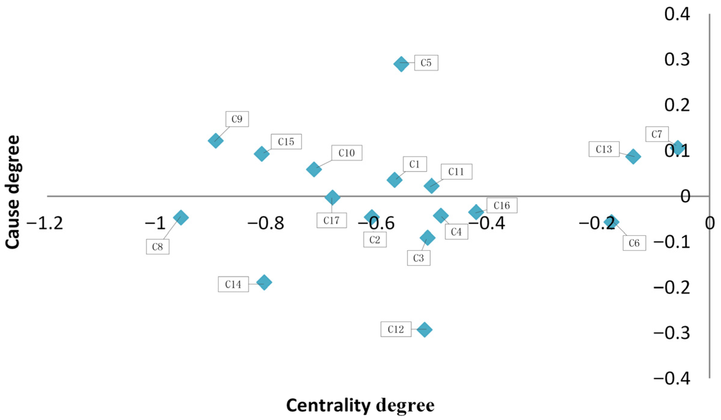
Figure 3 illustrates the causal relationships and importance of each criterion in the offshore oil and gas greenness assessment, using the dimensions of causality and centrality to describe the role of each criterion within the overall evaluation framework. Causality represents the extent to which a criterion influences other criteria, while centrality reflects the core position of the criterion within the overall evaluation system. The combination of these two dimensions provides us with an intuitive analytical framework, helping to identify which criteria play an important role in the decision-making process and which ones are more dependent on others. For example, criteria located in the negative region, such as C8 and C9, show that they are highly influenced by other criteria and have a smaller driving effect, playing a more marginal role, though their optimization still contributes to the environmental friendliness of the project. In contrast, criteria such as C5 and C17 have higher positive causality, indicating that they have a positive driving effect on other criteria. Optimizing these criteria may bring significant emission reduction benefits. Moreover, C8 has a high centrality, indicating that it holds a central position in the evaluation, and, despite its negative causality, its importance in energy consumption and emission control cannot be overlooked. On the other hand, criteria like C12 and C7 have lower centrality, which means that their contribution is smaller but still holds some reference value in terms of social impact or sustainability.
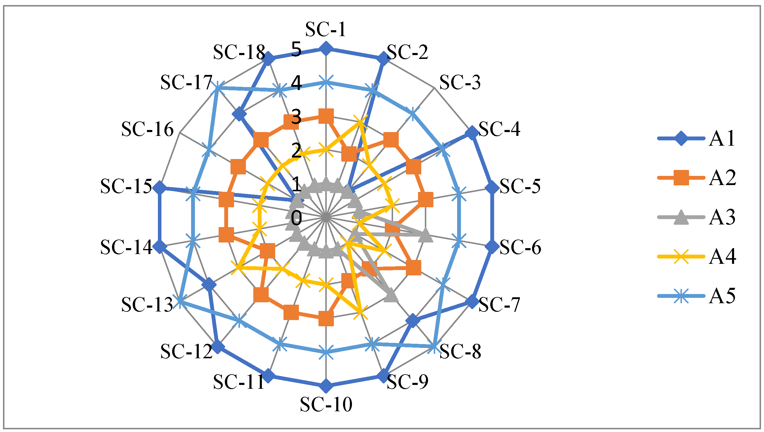
The SF–MAIRCA method was proposed to evaluate the five alternatives of the OOGFGP. The alternatives’ criteria values for the OOGFGP were evaluated using the SF scale (Table 5), relying on the judgment of experts. Table 17 lists the five OOGF extraction projects. Table 18 lists the assessment opinions of expert 1 considering the five alternatives. The criteria values for the other two experts’ evaluations are presented in Tables S3 and S4 in the Supplementary Materials. Table 19 shows the score function of the fuzzy matrix when using Equation (14). The theoretical evaluation matrix (Kp) was derived using Equation (24) and is displayed in Table 20. Based on Equations (25) and (26), the actual evaluation matrix (Kr) of OOGF project alternatives is calculated and displayed in Table 21. The total void matrix (G) is determined by Equation (30), which is shown as Table 22. The gap between the theoretical and actual evaluations of offshore oil and gas field project alternatives were calculated based on each criterion affecting the OOGFGP. The final values (Q) calculated for the five OOGF extraction projects were 0.109 for Huangyan 14-1 Gas Field Development Project (A1), 0.094 for Bozhong 28-2 South Oilfield Secondary Adjustment Project (A2), 0.067 for Lufeng 12-3 Oil Field Development Project (A3), 0.086 for Kenli 10-1 Oilfield and Surrounding Area Development Research Project (A4), and 0.113 for Kenli 3-2 Oilfield Cluster Development Project (A5). The order of Q value from smallest to largest is: A3 > A4 > A2 > A1 > A5. As Q is the direct difference between the ideal value and the real value, the smaller Q represents the better alternative, so the result shows that A3 is the most environmentally friendly OOGF extraction project.

4.2. Sensitivity Analysis

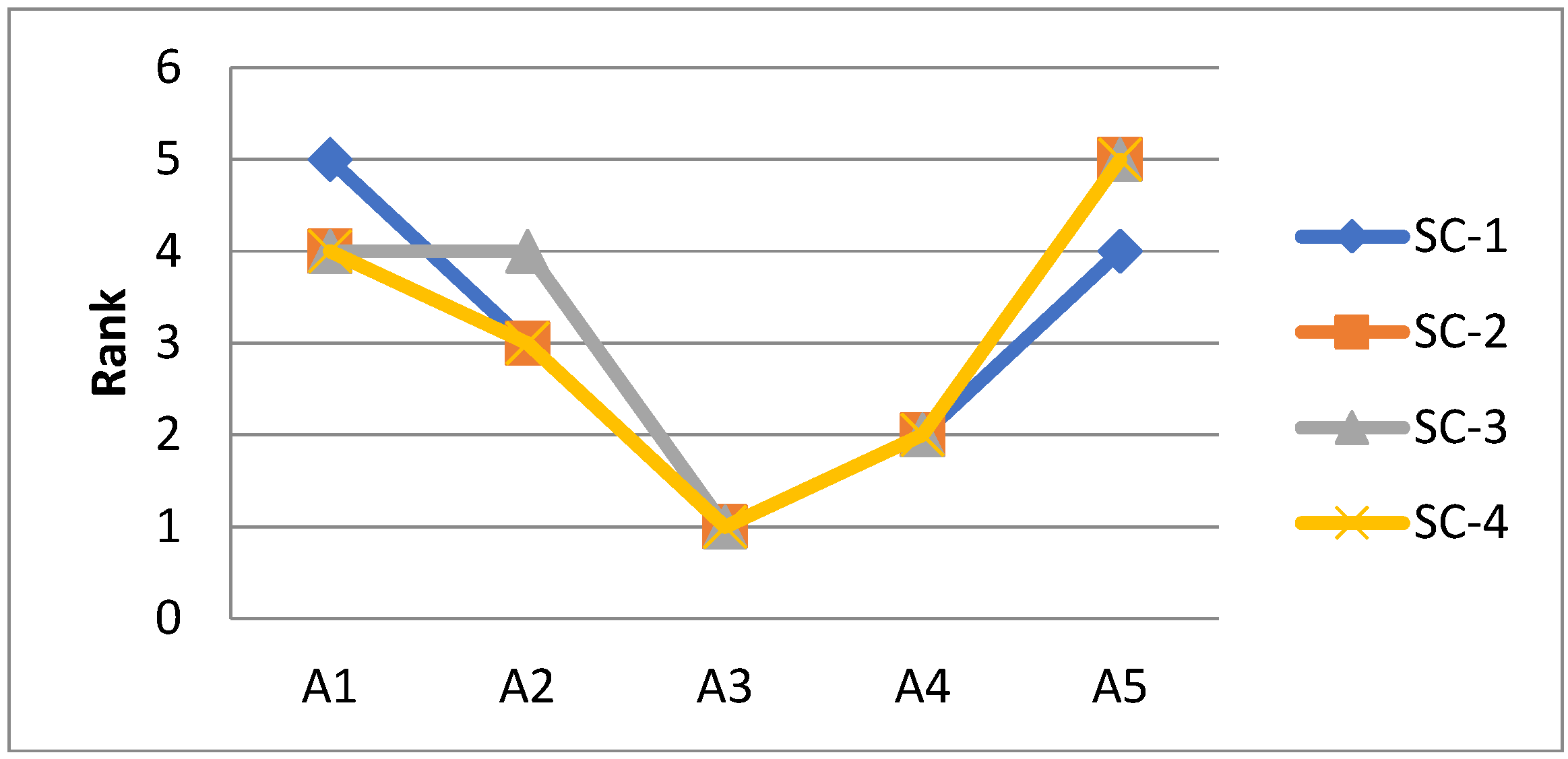
We performed a sensitivity analysis to check the reliability of our decision-making approach. We varied the importance given to each expert’s opinions to see how this affected the weights of different criteria. Four scenarios were considered with different weights assigned to three experts, which is shown in Table 23. In three of the scenarios, one expert had the most influence, while in the fourth scenario, all experts had equal influence.
We analyzed the sensitivity to changes in expert weights using the DEMATEL–MAIRCA integrated approach for the SF set, as demonstrated in Figure 4. In order to guarantee the dependability of our integrated approach, it was imperative to investigate the impact of criterion weight variations on the alternative ranking outcomes, particularly when the expert weights were equivalent. As depicted in Figure 4, the rankings of the five alternatives remain virtually unchanged across all four scenarios. The two most important alternatives are A2 (Bozhong 28-2 South Oilfield Secondary Adjustment Project) and A3 (Lufeng 12-3 Oil Field Development Project). This validates the stability of the DEMATEL–MAIRCA framework under the utilization of the SF sets, indicating its robustness and reliability in decision-making processes. Figure 5 shows the results of the sensitivity analysis, taking into account the change of the criteria weights. Table 24 demonstrates the results of the five OOGF extraction projects which exhibit variations in 18 distinct scenarios. This observation suggests that the SF–MAIRCA method is responsive to alterations in the assessment criteria. Consequently, the consolidation of SF–DEMATEL and SF–MAIRCA is justifiable for evaluating the OOGFGPs, ensuring a comprehensive and sensitive evaluation framework.

4.3. Comparative Analysis

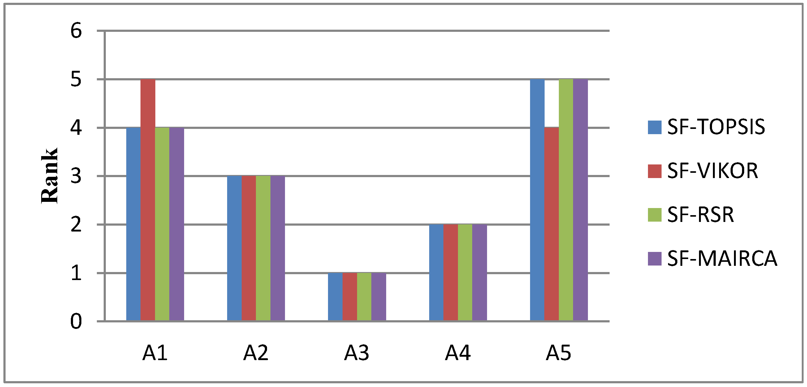
The weighting criteria were determined by applying SF–DEMATEL. Subsequently, SF–MAIRCA, SF–TOPSIS, SF–VIKOR, and SF–RSR were employed for further evaluation. Figure 6 and Table 25 present the amalgamated results of the assessment of the five alternatives using these four methodologies. Table 26 utilizes the Spearman rank correlation (SRC) to compare the ranking outcomes, revealing a robust positive correlation between the SF–MAIRCA rankings and those obtained from SF–TOPSIS, SF–VIKOR, and SF–RSR methods. Notably, the sequencing sequences derived from these three methods exhibit significant similarities.
However, in the SF–MAIRCA method, the five OOGF extraction projects are identified by measuring the difference between the ideal and empirical evaluations, which reduces the complexity of the computational process by using a linear normalization process and simple mathematical calculations. The SF–MAIRCA, SF–TOPSIS, SF–VIKOR, and SF–RSR methods identify the two most important alternatives, which are A2 (Bozhong 28-2 South Oilfield Secondary Adjustment Project) and A3 (Lufeng 12-3 Oil Field Development Project). Furthermore, the SF–MAIRCA method demonstrates consistency in identifying less significant alternatives, which validates the applicability and effectiveness of the proposed integration methodology. This consistency strengthens the reliability of the method in practical scenarios.

5. Discussion

5.1. Interpretation of the Ranking: Project Characteristics and Environmental Performance

The ranking hierarchy (A3 > A4 > A2 > A1 > A5) reflects fundamental differences in project type, development phase, and operational configuration, which collectively determine environmental outcomes.
A3 (Lufeng 12-3) emerged as the top performer, consistent with its characterization as a new development project. New builds benefit from technological lock-in advantages: they can incorporate best-available energy-efficient equipment (C8, C10), integrate renewable energy sources (C6) more readily than brownfield projects, and are designed to meet contemporary emission standards from inception. In the Bohai Bay context, where stringent environmental regulations apply uniformly, newer projects face lower retrofitting costs and compliance burdens, explaining their superior environmental profile.
A4 (Kenli 10-1), classified as a research project, ranked second. While still in the planning phase, its position reflects the inherent environmental advantage of “design flexibility.” Research-phase projects can incorporate emerging low-carbon technologies, optimize facility layouts to minimize transportation emissions (C16), and conduct comprehensive environmental impact assessments before construction commences. This finding underscores the critical importance of integrating environmental considerations early in the project lifecycle—a principle increasingly emphasized in offshore oil and gas environmental management frameworks.
A2 (Bozhong 28-2 South), a secondary adjustment project, occupied the middle position. Secondary recovery operations typically involve increased water handling and enhanced compression requirements, which elevate energy consumption and associated emissions. However, as an adjustment of existing infrastructure, A2 retains some mitigation potential through equipment upgrades, placing it ahead of fully operational fields with limited modification scope. This result highlights the environmental trade-offs inherent in extending field life: while secondary recovery improves resource utilization efficiency, it inevitably increases operational environmental intensity.
A1 (Huangyan 14-1), a gas field development, ranked fourth—a finding that merits careful interpretation. While natural gas combustion produces lower local air pollutants (C3) than oil, gas fields present distinct environmental challenges, particularly regarding methane fugitive emissions. Methane’s global warming potential is approximately 28–34 times that of CO2 over a 100-year period, meaning that even small leakage rates can substantially increase a project’s climate impact. The expert ranking appropriately captures this nuance: despite cleaner combustion characteristics, A1’s potential methane leakage from wet gas compressors (C10) and processing facilities likely elevates its overall greenhouse gas intensity (C11), justifying its position below A2 and A4. This finding aligns with growing scientific consensus that natural gas infrastructure requires rigorous leak detection and repair programs to realize its climate benefits.
A5 (Kenli 3-2 Cluster) ranked lowest, consistent with the environmental penalties associated with cluster development configurations. Cluster developments typically involve multiple small platforms tied back to central processing facilities, necessitating frequent transportation (C16) between sites, increased diesel generator usage for remote platforms (C7), and greater spatial footprint within sensitive marine ecosystems. In the Bohai Bay context—a semi-enclosed sea with limited water exchange and high cumulative pollution loads—cluster developments exacerbate environmental stress through distributed emissions and intensified logistical activity. The low ranking also reflects anticipated stakeholder opposition (C12, C13) from coastal communities and fisheries, which are particularly sensitive to cumulative impacts in densely developed marine areas.

5.2. Policy Scenario Testing: Implications for Energy Transition Pathways

The electrification scenario analysis provides critical insights into how ongoing energy transition policies may reshape project-level environmental competitiveness. Under the Bohai Bay shore power initiative—which aims to replace platform-based power generation with grid-supplied electricity—all projects demonstrated improved environmental scores, confirming the policy’s intended effectiveness. However, the magnitude of improvement varied systematically across projects, with A3 and A4 showing the largest gains (+4.2%) and A5 the smallest (+2.1%).
This differential responsiveness carries important implications for environmental management and investment planning:
First, the results suggest that newer and research-phase projects are better positioned to benefit from grid decarbonization. As the North China Grid gradually reduces its carbon intensity through renewable energy integration, projects with shore power connectivity and modern electrical infrastructure will experience compounding environmental benefits. This “green dividend” of new builds reinforces the economic case for early-stage environmental investments.
Second, the relatively modest improvement for A5 under electrification (+2.1%) reflects the structural constraints of cluster developments. Remote satellite platforms may lack feasible shore power connections due to distance from main grids or high transmission losses, potentially requiring continued reliance on diesel generation. This finding suggests that policy interventions may need to be tailored to project configurations, with cluster developments requiring alternative decarbonization pathways such as localized renewable microgrids or advanced energy storage.
Third, the stability of the ranking across scenarios (no positional changes) indicates that current environmental performance is a robust predictor of future policy compatibility. Projects that rank higher under baseline conditions are also better positioned to adapt to tightening environmental regulations—a property we term “policy resilience”. This resilience has practical implications for investment decisions, regulatory approvals, and environmental due diligence in the offshore oil and gas sector.

6. Conclusions

In the context of carbon neutrality and carbon peaking, it has become a great challenge to build and develop sustainable offshore oil and gas fields in a green way. The OOGFGP aims to realize a win–win situation between production and environmental protection by adopting cleaner production technologies, circular economy models and energy-saving and environmental protection measures. Evaluating OOGFGP is of great significance for implementing green manufacturing, accelerating the green transformation and development of the manufacturing industry, and promoting the stable growth of the industry. Evaluation of the OOGFGP requires multiple interacting criteria. Therefore, evaluating OOGFGP also falls within the scope of research on MCDM. Considering the importance of energy sustainability and green development in OOGF extraction projects, this paper proposes an OOGFGP evaluation model based on SF–DEMATEL–MAIRCA. The most important contributions can be counted as follows: (1) In this paper, a comprehensive evaluation criteria system is constructed for the OOGFGP. (2) The paper proposes the DEMATEL–MAIRCA method under SF sets to evaluate the OOGFGP. This method takes into account the judgment and preference information of decision makers in a comprehensive manner, thereby facilitating rational evaluation and modeling of decision-making problems.
The limitation of this study is the use of fuzzy sets to deal with the information uncertainty of expert evaluation, which does not take into account the experts’ preference. In addition, this study only investigated the evaluation of green factories in offshore oil and gas fields and did not investigate the impact projects such as renewable energy utilization. Moreover, while this study primarily concentrates on green factory evaluation, several key offshore issues were not included in the evaluation framework.
Therefore, the following studies can be carried out in future research: (i) Consider the introduction of regret theory for the assessment of green factories in OOGFs; (ii) investigate the projects in conjunction with objective data for further assessment and calculation; and (iii) consider incorporating key issues such as methane emissions, flaring/venting, produced water impacts, spill preparedness, and decommissioning into the evaluation framework for a more comprehensive assessment.


Supplementary Materials

The following supporting information can be downloaded at: https://www.mdpi.com/article/10.3390/en19061398/s1, Table S1: Judgement opinions of expert-2 regarding the 17 criteria; Table S2: Judgement opinions of expert-3 regarding the 17 criteria; Table S3: Judgement opinions of expert-2 regarding the 5 alternatives; Table S4: Judgement opinions of expert-3 regarding the 5 alternatives.

Author Contributions

Y.Z.: Conceptualization, validation, formal analysis, data curation, investigation, writing—original draft. X.G.: Writing—review and editing, conceptualization, funding acquisition, resources, supervision. Y.D.: Conceptualization, software, writing—review and editing. W.Z.: Project administration, resources, writing—review and editing. All authors have read and agreed to the published version of the manuscript.

Funding

This research was supported by the National Natural Science Foundation Committee (NSFC) of China (No. 72271164).

Data Availability Statement

Data will be made available on request.

Acknowledgments

This research was supported by the National Natural Science Foundation Committee (NSFC) of China (No. 72271164), as well as the contributions from all collaborators within the projects mentioned.

Conflicts of Interest

The authors declare no conflicts of interest.

References

  1. Crivellari, A.; Bonvicini, S.; Tugnoli, A.; Cozzani, V. Multi-target inherent safety indices for the early design of offshore oil & gas facilities. Process Saf. Environ. Prot. 2021, 148, 256–272. [Google Scholar]
  2. Nguyen, T.V.; Voldsund, M.; Breuhaus, P.; Elmegaard, B. Energy efficiency measures for offshore oil and gas platforms. Energy 2016, 117, 325–340. [Google Scholar] [CrossRef] [Scilit]
  3. International Energy Agency. Global Methane Tracker 2025. 2025. Available online: https://www.iea.org/reports/global-methane-tracker-2025 (accessed on 25 December 2025).
  4. Mohammadi, S.; Berg, C.F.; Schümann, H. Low-emission offshore oil and gas production: A review of achievements and challenges. J. Clean. Prod. 2025, 525, 146504. [Google Scholar] [CrossRef] [Scilit]
  5. Wu, Y.; Zhang, J.; Yuan, J.; Geng, S.; Zhang, H. Study of decision framework of offshore wind power station site selection based on ELECTRE-III under intuitionistic fuzzy environment: A case of China. Energy Convers. Manag. 2016, 113, 66–81. [Google Scholar] [CrossRef] [Scilit]
  6. Zhang, X.; Lu, J.; Peng, Y. Hybrid MCDM model for location of logistics hub: A case in China under the Belt and Road Initiative. IEEE Access 2021, 9, 41227–41245. [Google Scholar] [CrossRef] [Scilit]
  7. Zou, X.; Qiu, R.; Yuan, M.; Liao, Q.; Yan, Y.; Liang, Y.; Zhang, H. Sustainable offshore oil and gas fields development: Techno-economic feasibility analysis of wind–hydrogen–natural gas nexus. Energy Rep. 2021, 7, 4470–4482. [Google Scholar] [CrossRef] [Scilit]
  8. Lima De, Y.Q.; Gomes, L.F.; Leoneti, A.B. Towards the Green Economy: An MCDA approach to decommissioning offshore oil and gas production systems. Procedia Comput. Sci. 2022, 214, 337–343. [Google Scholar] [CrossRef] [Scilit]
  9. Ivanega, D.; Szczepanek, M. Assessing damage and predicting future risks: A study of the Schilling Titan 4 manipulator on work class ROVs in offshore oil and gas industry. Ocean Eng. 2024, 291, 116282. [Google Scholar] [CrossRef] [Scilit]
  10. Li, Y.; Hu, Z. Application of Hierarchical Analyst Domino Evaluation System (HADES) in offshore oil and gas facilities’ decommissioning: A case study. Ocean Eng. 2023, 272, 113741. [Google Scholar] [CrossRef] [Scilit]
  11. Vidal, P.D.; González, M.O.; de Vasconcelos, R.M.; de Melo, D.C.; de Oliveira Ferreira, P.; Sampaio, P.G.; da Silva, D.R. Decommissioning of offshore oil and gas platforms: A systematic literature review of factors involved in the process. Ocean Eng. 2022, 255, 111428. [Google Scholar] [CrossRef] [Scilit]
  12. Lian, J.; Hou, G.; Cai, O.; Xu, K. Assessing the life cycle risks of offshore wind turbines with suction bucket foundations. J. Clean. Prod. 2022, 362, 132366. [Google Scholar] [CrossRef] [Scilit]
  13. Önden, İ.; Kara, K.; Yalçın, G.C.; Deveci, M.; Önden, A.; Eker, M. Strategic location analysis for offshore wind farms to sustainably fulfill railway energy demand in Turkey. J. Clean. Prod. 2024, 434, 140142. [Google Scholar] [CrossRef] [Scilit]
  14. Gil-García, I.C.; Ramos-Escudero, A.; Molina-García, Á.; Fernández-Guillamón, A. GIS-based MCDM dual optimization approach for territorial-scale offshore wind power plants. J. Clean. Prod. 2023, 428, 139484. [Google Scholar] [CrossRef] [Scilit]
  15. Shao, M.; Han, Z.; Sun, J.; Gao, H.; Zhang, S.; Zhao, Y. A novel framework for wave power plant site selection and wave forecasting based on GIS, MCDM, and ANN methods: A case study in Hainan Island, Southern China. Energy Convers. Manag. 2024, 299, 117816. [Google Scholar] [CrossRef] [Scilit]
  16. Nasrollahi, S.; Kazemi, A.; Jahangir, M.H.; Aryaee, S. Selecting suitable wave energy technology for sustainable development, an MCDM approach. Renew. Energy 2023, 202, 756–772. [Google Scholar] [CrossRef] [Scilit]
  17. Zhou, Q.; Ye, C.; Geng, X. A decision framework of offshore wind power station site selection using a MULTIMOORA method under Pythagorean hesitant fuzzy environment. Ocean Eng. 2024, 291, 116416. [Google Scholar] [CrossRef] [Scilit]
  18. Cali, U.; Kantar, E.; Pamucar, D.; Deveci, M.; Taylor, P.; Campos-Gaona, D.; Anaya-Lara, O.; Tande, J.O. Offshore wind farm site selection in Norway: Using a fuzzy trigonometric weighted assessment model. J. Clean. Prod. 2024, 436, 140530. [Google Scholar] [CrossRef] [Scilit]
  19. Golestani, N.; Arzaghi, E.; Abbassi, R.; Garaniya, V.; Abdussamie, N.; Yang, M. The Game of Guwarra: A game theory-based decision-making framework for site selection of offshore wind farms in Australia. J. Clean. Prod. 2021, 326, 129358. [Google Scholar] [CrossRef] [Scilit]
  20. Ling, L.; Wang, X.; Zhang, L.; Zhang, Z.; Koh, L.H. Fuzzy control based virtual synchronous generator for self-adaptative control in hybrid microgrid. Energy Rep. 2022, 8, 12092–120104. [Google Scholar] [CrossRef] [Scilit]
  21. Zadeh, L.A. (Ed.) A note on prototype theory and fuzzy sets. In Fuzzy Sets, Fuzzy Logic, and Fuzzy Systems: Selected Papers by Lotfi A Zadeh; World Scientific Publishing Co Pte Ltd.: Singapore, 1996; pp. 587–593. [Google Scholar]
  22. Atanassov, K.T. Geometrical interpretation of the elements of the intuitionistic fuzzy objects. Int. J. Bioautom. 2016, 20, S27–S42. [Google Scholar]
  23. Yager, R.R. Pythagorean membership grades in multicriteria decision making. IEEE Trans. Fuzzy Syst. 2013, 22, 958–965. [Google Scholar] [CrossRef] [Scilit]
  24. Kumar, R.; Gandotra, N. Novel Pythagorean Fuzzy Entropy with Application in MCDM to assess the Best Automotive Company. In Proceedings of the 2021 8th International Conference on Computing for Sustainable Global Development (INDIA-Com), New Delhi, India, 17–19 March 2021; pp. 167–171. [Google Scholar]
  25. Thakur, P.; Kizielewicz, B.; Gandotra, N.; Shekhovtsov, A.; Saini, N.; Sałabun, W. The group decision-making using Pythagorean fuzzy entropy and the complex proportional assessment. Sensors 2022, 22, 4879. [Google Scholar] [CrossRef] [Scilit] [PubMed]
  26. Kutlu Gündoğdu, F.; Kahraman, C. Spherical fuzzy sets and spherical fuzzy TOPSIS method. J. Intell. Fuzzy Syst. 2019, 36, 337–352. [Google Scholar] [CrossRef] [Scilit]
  27. Uygun, Ö.; Kaçamak, H.; Kahraman, Ü.A. An integrated DEMATEL and Fuzzy ANP techniques for evaluation and selection of outsourcing provider for a telecommunication company. Comput. Ind. Eng. 2015, 86, 137–146. [Google Scholar] [CrossRef] [Scilit]
  28. Tzeng, G.H.; Chiang, C.H.; Li, C.W. Evaluating intertwined effects in e-learning programs: A novel hybrid MCDM model based on factor analysis and DEMATEL. Expert Syst. Appl. 2007, 32, 1028–1044. [Google Scholar] [CrossRef] [Scilit]
  29. Gül, S. Spherical fuzzy extension of DEMATEL (SF-DEMATEL). Int. J. Intell. Syst. 2020, 35, 1329–1353. [Google Scholar] [CrossRef] [Scilit]
  30. Zhu, X.; Ran, Y.; Zhang, G.; Chen, J.; Heli, L. Identification of maintenance significant items for machine tools by integrating DEMATEL and MABAC with spherical fuzzy sets. Eng. Appl. Artif. Intell. 2023, 126, 107155. [Google Scholar] [CrossRef] [Scilit]
  31. Büyüközkan, G.; Karabulut, Y.; Göçer, F. Spherical Fuzzy Sets based Integrated DEMATEL, ANP, VIKOR Approach and its application for Renewable Energy Selection in Turkey. Appl. Soft Comput. 2024, 7, 111465. [Google Scholar] [CrossRef] [Scilit]
  32. Erdoğan, M.; Kaya, İ.; Karaşan, A.; Çolak, M. Evaluation of autonomous vehicle driving systems for risk assessment based on three-dimensional uncertain linguistic variables. Appl. Soft Comput. 2021, 113, 107934. [Google Scholar] [CrossRef] [Scilit]
  33. Pamučar, D.; Vasin, L.; Lukovac, L. Selection of railway level crossings for investing in security equipment using hybrid DEMATEL-MARICA model. In Proceedings of the XVI International Scientific-Expert Conference on Railways, Niš, Serbia, 9–10 October 2014; pp. 89–92. [Google Scholar]
  34. Boral, S.; Howard, I.; Chaturvedi, S.K.; McKee, K.; Naikan, V.N. An integrated approach for fuzzy failure modes and effects analysis using fuzzy AHP and fuzzy MAIRCA. Eng. Fail. Anal. 2020, 108, 104195. [Google Scholar] [CrossRef] [Scilit]
  35. Haq, R.S.; Saeed, M.; Mateen, N.; Siddiqui, F.; Ahmed, S. An interval-valued neutrosophic based MAIRCA method for sustainable material selection. Eng. Appl. Artif. Intell. 2023, 123, 106177. [Google Scholar] [CrossRef] [Scilit]
  36. Dınçer, H.; Etı, S.; Aksoy, T.; Yüksel, S.; Hacioglu, U.; Mikhaylov, A.; Muyeen, S.M. Analysis of environmental impact for material production investments using a novel soft computing methodology. IEEE Access 2023, 11, 37987–38001. [Google Scholar] [CrossRef] [Scilit]
  37. Ministry of Industry and Information Technology. National Standard for Green Factory Evaluation General Rules Officially Released. 2018. Available online: https://www.miit.gov.cn/xwdt/gxdt/sjdt/art/2020/art_82394633cc3844e186233e20fae7185f.html (accessed on 20 December 2025).
  38. Iaiani, M.; Tugnoli, A.; Cozzani, V.; Reniers, G.; Yang, M. A Bayesian-network approach for assessing the probability of success of physical security attacks to offshore Oil & Gas facilities. Ocean Eng. 2023, 273, 114010. [Google Scholar]
  39. Almedallah, M.K.; Walsh, S.D. A numerical method to optimize use of existing assets in offshore natural gas and oil field developments. J. Nat. Gas Sci. Eng. 2019, 67, 43–55. [Google Scholar] [CrossRef] [Scilit]
  40. D’Antoine, E.; Jansz, J.; Barifcani, A.; Shaw-Mills, S.; Harris, M.; Lagat, C. COVID-19 and offshore oil and gas workers: The role of personality. Soc. Sci. Hum. Open 2023, 7, 100402. [Google Scholar] [CrossRef] [Scilit] [PubMed]
  41. Socolofsky, S.A.; Jun, I.; Boufadel, M.C.; Liu, R.; Lu, Y.; Arey, J.S.; McFarlin, K.M. Development of an offshore response guidance tool for determining the impact of SSDI on released gas and benzene from artificial subsea oil well blowout simulations. Mar. Pollut. Bull. 2022, 184, 114114. [Google Scholar] [CrossRef] [Scilit] [PubMed]
  42. Iaiani, M.; Moreno, C.; Reniers, G.; Tugnoli, A.; Cozzani, V. Analysis of events involving the intentional release of hazardous substances from industrial facilities. Reliab. Eng. Syst. Saf. 2021, 212, 107593. [Google Scholar] [CrossRef] [Scilit]
  43. Beyer, J.; Goksøyr, A.; Hjermann, D.Ø.; Klungsøyr, J. Environmental effects of offshore produced water discharges: A review focused on the Norwegian continental shelf. Mar. Environ. Res. 2020, 162, 105155. [Google Scholar] [CrossRef] [Scilit]
  44. Farmer, N.A.; Baker, K.; Zeddies, D.G.; Denes, S.L.; Noren, D.P.; Garrison, L.P.; Machernis, A.; Fougères, E.M.; Zykov, M. Population consequences of disturbance by offshore oil and gas activity for endangered sperm whales (Physeter macrocephalus). Biol. Conserv. 2018, 227, 189–204. [Google Scholar] [CrossRef] [Scilit]
  45. Yacovitch, T.I.; Daube, C.; Herndon, S.C. Methane emissions from offshore oil and gas platforms in the Gulf of Mexico. Environ. Sci. Technol. 2020, 54, 3530–3538. [Google Scholar] [CrossRef] [Scilit]
  46. Thomas, C.; Stillman, S.; Davis, P.; Mahon, I.; Horstmann, B.; Raphael, J.; Moreau, K.; Teller, E.; Franklin, K.; Kroodsma, D. Exposing the Environmental Costs of Offshore Oil: Greenhouse Gas Emissions, Oil Slicks, and Flaring. In Proceedings of the One Ocean Science Congress 2025, Nice, France, 3–6 June 2025. No. OOS2025-733. [Google Scholar]
  47. Ekins, P.; Vanner, J. Decommissioning of offshore oil and gas facilities: A comparative assessment of different scenarios. J. Environ. Manag. 2006, 79, 420–438. [Google Scholar] [CrossRef] [Scilit] [PubMed]
  48. Vidal, P.D.; González, M.O.; de Melo, D.C.; de Oliveira Ferreira, P.; Sampaio, P.G.; Lima, L.O. Conceptual framework for the decommissioning process of offshore oil and gas platforms. Mar. Struct. 2022, 85, 103262. [Google Scholar] [CrossRef] [Scilit]
  49. Banihabib, R.; Assadi, M. Towards a low-carbon future for offshore oil and gas industry: A smart integrated energy management system with floating wind turbines and gas turbines. J. Clean. Prod. 2023, 423, 138742. [Google Scholar] [CrossRef] [Scilit]
  50. Piscopo, V.; Scamardella, A. Incidence of wind spectrum and turbulence intensity on the design of mooring systems for floating offshore wind turbines. Ocean Eng. 2023, 290, 116377. [Google Scholar] [CrossRef] [Scilit]
  51. Ozowe, W.; Ikevuje, A.H.; Ogbu, A.D.; Esiri, A.E. Renewable energy integration in offshore oil and gas installations. Magna Sci. Adv. Res. Rev. 2023, 8, 238–250. [Google Scholar] [CrossRef] [Scilit]
  52. Amaral, J.M.; Ramos, J.S.; van Emmerik, E.L.; Dias, R.F. Assessment of offshore wind turbine controls for integration with offshore oil & gas platforms. In 2024 4th International Conference on Smart Grid and Renewable Energy (SGRE), Doha, Qatar, 8–10 January 2024; pp. 1–6. [Google Scholar]
  53. Liu, G.; Kong, Z.; Sun, W.; Li, J.; Qi, Z.; Wu, C.; Li, C. Impacts of offshore wind power development on China’s marine economy and environment: A study from 2006 to 2019. J. Clean. Prod. 2023, 423, 138618. [Google Scholar] [CrossRef] [Scilit]
  54. Masnadi, M.S.; Brandt, A.R. Climate impacts of oil extraction increase significantly with oilfield age. Nature Clim. Change 2017, 7, 551–556. [Google Scholar] [CrossRef] [Scilit]
  55. Nienhuis, R.M.; van Rooij, M.; Prins, W.A.; Jayawardhana, B.; Vakis, A.I. Investigating the efficiency of a novel offshore pumped hydro energy storage system: Experimental study on a scale prototype. J. Energy Storage 2023, 74, 109374. [Google Scholar] [CrossRef] [Scilit]
  56. Santos, E. Innovative solutions for coastal and offshore infrastructure in seawater mining: Enhancing efficiency and environmental performance. Desalination 2024, 14, 117282. [Google Scholar] [CrossRef] [Scilit]
  57. Kong, X.; Wang, W.; Liu, X.; Ma, L.; Abdelbaky, M.A.; Lee, K.Y. Offshore wind turbines real-time control using convex nonlinear economic MPC scheme. Ocean Eng. 2024, 297, 116988. [Google Scholar] [CrossRef] [Scilit]
  58. Tuy, S.; Lee, H.S.; Chreng, K. Integrated assessment of offshore wind power potential using Weather Research and Forecast (WRF) downscaling with Sentinel-1 satellite imagery, optimal sites, annual energy production, and equivalent CO2 reduction. Renew. Sustain. Energy Rev. 2022, 163, 112501. [Google Scholar] [CrossRef] [Scilit]
  59. Hooper, T.; Ashley, M.; Austen, M. Perceptions of fishers and developers on the co-location of offshore wind farms and decapod fisheries in the UK. Mar. Policy 2015, 61, 16–22. [Google Scholar] [CrossRef] [Scilit]
  60. Andrews, N.; Bennett, N.J.; Le Billon, P.; Green, S.J.; Cisneros-Montemayor, A.M.; Amongin, S.; Gray, N.J.; Sumaila, U.R. Oil, fisheries and coastal communities: A review of impacts on the environment, livelihoods, space and governance. Energy Res. Soc. Sci. 2021, 75, 102009. [Google Scholar] [CrossRef] [Scilit]
  61. Mukherjee, D.; Rahman, M.A. To drill or not to drill? An econometric analysis of US public opinion. Energy Policy 2016, 91, 341–351. [Google Scholar] [CrossRef] [Scilit]
  62. Gkeka-Serpetsidaki, P.; Tsoutsos, T. Integration criteria of offshore wind farms in the landscape: Viewpoints of local inhabitants. J. Clean. Prod. 2023, 417, 137899. [Google Scholar] [CrossRef] [Scilit]
  63. Mason, C.F. Public policy towards offshore oil projects: Confronting potential deepwater oil spills. J. Environ. Manag. 2024, 372, 123315. [Google Scholar] [CrossRef] [Scilit]
  64. Taleghani, N.D.; Tyagi, M. Impacts of major offshore oil spill incidents on the petroleum industry and regional economy. J. Energy Res. Technol. 2017, 139, 022913. [Google Scholar] [CrossRef] [Scilit]
  65. Bamidele, B. Review of the Hazards and Management Control Issues in Abandonment Safety Cases; Lloyd’s Register System Integrity and Risk Management: Croydon, UK, 1997. [Google Scholar]
  66. Li, Y.; Hu, Z. MADM-Q, an efficient multi-attribute decision-making support system for offshore decommissioning. Ocean Coast. Manag. 2023, 243, 106732. [Google Scholar] [CrossRef] [Scilit]
  67. Dalalah, D.; Hayajneh, M.; Batieha, F. A fuzzy multi-criteria decision making model for supplier selection. Expert Syst. Appl. 2011, 38, 8384–8391. [Google Scholar] [CrossRef] [Scilit]
Figure 1. Evaluation criteria system for OOGFGP.
Energies 19 01398 g001
Figure 2. The framework for the evaluation of offshore oil and gas field green plants.
Energies 19 01398 g002
Figure 3. The cause result diagram of the criteria.
Energies 19 01398 g003
Figure 4. Results of sensitivity analysis with changing expert weights.
Energies 19 01398 g004
Figure 5. Results of sensitivity analysis with changing criteria weights.
Energies 19 01398 g005
Figure 6. Combined results of the evaluation of the five alternatives using these four methods.
Energies 19 01398 g006
Table 1. Studies regarding OOGFs and offshore manufacturing.
AuthorMethodResearch
[7]Technical and economic evaluation modelsEvaluation framework for offshore oil and gas fields
[8]ExpTODIMDecommissioning analysis of an offshore oil and gas production system
[9]Questionnaire and Geogebra programDamage assessment and risk prediction for underwater vehicles in the offshore oil and gas industry
[10]Hierarchical analyst domino evaluation systemDecommissioning process of offshore oil platforms
[11]A systematic analysisDecommissioning process of offshore oil platforms
[12]Fuzzy fault tree analysisAssessment of the life cycle risks of offshore wind turbines
[13]SF-SWARA and Einstein’s arithmetic t-norm techniqueOffshore wind farm site selection
[14]AHP and EntropyOffshore wind power plants siting
[15]AHP-TOPSISWave power plant siting on Hainan Island
[16]FDM and PROMETHEEWave energy technologies evaluation as alternatives in the ocean
[17]SWARA and the extended MULTIMOORAOffshore wind farms siting
[18]TRWAOffshore wind farms siting
[19]Decision-support toolDevelopment of an offshore wind power plant in the Bass Strait
Table 2. Detailed information regarding evaluation criteria.
Evaluation CriteriaMeasurement Scale/UnitTypeSource
Water pollutant emissions (C1)Ton/yearCost[43]
Noise emissions (C2)dBCost[44]
Air pollutant emissions (C3)Ton/yearCost[45,46]
Extreme weather and sea conditions (C4)m/sCost[47,48]
Monthly wind velocity (C5)m/sCost[49,50]
Renewable energy use (C6)kWhBenefit[51,52]
High pollutant use (C7)Ton/yearCost[53]
Energy efficiency of sea water pumps (C8)kWh/m3Benefit[55,56]
Wind turbine linear capacity related costs (C9)USD/kWCost[49,57]
Energy efficiency of dry/wet gas compressors (C10)kWh/m3Benefit[56]
CO2 equivalent intensity (C11)g CO2e/kWhCost[58]
Attitudes of coastal residents and fishermen (C12)% (Percentage of support based on attitude)Benefit[59,60]
Attitudes of government (C13)% (Percentage of support based on attitude)Benefit[63]
Equipment renting and application license fee (C14)USDCost[65,66]
Diving equipment (C15)Number of equipmentBenefit[9,10]
Transportation (C16)USD/kmBenefit[65,66]
Accident early warning (C17)Incidents per yearBenefit[1]
Table 3. The meanings of notations.
Notation List
XUniverse of discourse z i j k Element of Z ˜ s
A ˜ s An SF set D ˜ s = ( D ˜ μ , D ˜ ν , D ˜ π ) Normalized initial direct relation matrix
μ A ˜ s Degree of membership d i j μ Element of D ˜ μ
ν A ˜ s Degree of non-membership T ˜ s = ( T ˜ μ , T ˜ ν , T ˜ π ) Total influence matrix
π A ˜ s Degree of hesitancy E ˜ i Sum of rows of T ˜ s
δ A ˜ s Degree of refusal R ˜ j Sum of columns of T ˜ s
cCriteria seteExpert set
NNumber of criteriaKNumber of experts
w i j Weight of criterion Z ˜ s = ( Z ˜ μ , Z ˜ ν , Z ˜ π ) Average matrix
Table 4. SF scales and linguistic terms for evaluating criteria.
Linguistic Terms ( μ , ν , π )
Serious influence (SE)(0.9, 0.1, 0.1)
Extreme influence (EX)(0.8, 0.2, 0.2)
Major influence (MA)(0.7, 0.3, 0.3)
Significant influence (SI)(0.6, 0.4, 0.4)
Medium influence (ME)(0.5, 0.5, 0.5)
Minor influence (MI)(0.4, 0.6, 0.4)
Slight influence (SL)(0.3, 0.7, 0.3)
Remote influence (RE)(0.2, 0.8, 0.2)
No influence (NO)(0.1, 0.9, 0.1)
Table 5. SF scales and linguistic terms for evaluating alternatives.
Linguistic TermsSF Number
Almost no significance (AN)[0.045, 0.955, 0.045]
Extremely low significance (EL)[0.135, 0.865, 0.135]
Very low significance (VL)[0.255, 0.745, 0.255]
Low significance (L)[0.335, 0.665, 0.335]
Fair significance (F)[0.410, 0.590, 0.410]
Medium significance (M)[0.500, 0.500, 0.500]
Moderately high significance (MH)[0.590, 0.410, 0.410]
High significance (H)[0.665, 0.335, 0.335]
Very high significance (VH)[0.745, 0.255, 0.255]
Extremely high significance (EH)[0.865, 0.135, 0.135]
Almost equal significance (AE)[0.955, 0.045, 0.045]
Table 6. Judgement opinions of expert 1 regarding the 17 criteria.
CriteriaC1C2C3C4C5C6C7C8C9C10C11C12C13C14C15C16C17
C10REMAMASIMAMAMINOSIEXSEMAMEMAMESI
C2RE0RESIMIMAMAMAMAMINOEXMAMEMEMAMA
C3MARE0MAMIMAMAMINOSLEXSEMAMEMEMEMA
C4REMIME0MAMEMEMIREMAMISEMAMAMAMASE
C5MAMAMAMA0MASIMIEXSLSIMAMAMAMEMAMA
C6MAMAMAMAMI0MAMAMAMAEXSIMAMAMEMASI
C7MAMAEXEXMAMA0MAMAMAEXSEMAMAMEMASI
C8MEMARESIMESISI0REMISIREMEMAREMEMI
C9MEMAMAREEXMAMARE0RESIMESIMAREMERE
C10REMAMAMAMAMAMARERE0SIRESIMAMEMEMI
C11MANOMAEXSIMAMASLMESI0MASIREMEMAMA
C12MEMEMEREREMEMEMIMIMIMI0MEREMEMESI
C13SESESEMARESESEMESIMESIMA0SIRESIMA
C14MEREREMIMIMAMAMIMIMIRERESI0MEMARE
C15MAMAMIMIMEMAMASLSLSLSISIMIRE0MESI
C16MIMASIMIMAMAMASISISISIMAMEMESI0RE
C17MEMASIMAMIMEMEMEREMEMESIMASLMAMA0
Table 7. Average influence matrix Zμ.
ZμC1C2C3C4C5C6C7C8C9C10C11C12C13C14C15C16C17
C10.0000.1740.6120.6710.5110.6480.739 0.411 0.174 0.570 0.772 0.8210.7390.5000.5450.5000.612
C20.1740.0000.1740.6710.3710.6710.638 0.671 0.739 0.437 0.174 0.8420.7390.5000.5000.6710.671
C30.6120.1740.0000.7000.4700.6710.638 0.411 0.174 0.491 0.821 0.8210.7000.5000.4110.5000.671
C40.2860.3710.5000.0000.7960.5000.500 0.411 0.174 0.648 0.411 0.8420.7390.7000.6710.7390.821
C50.7000.7390.7390.6710.0000.6710.511 0.371 0.772 0.491 0.570 0.6710.6380.6380.5000.6710.739
C60.7390.6710.7000.6380.3710.0000.739 0.671 0.739 0.671 0.772 0.6120.6380.6120.5000.6710.511
C70.7720.6380.8420.8210.6380.7720.000 0.671 0.671 0.638 0.821 0.8210.7390.6380.5000.6710.511
C80.5000.6710.1740.5110.4700.5700.570 0.000 0.174 0.371 0.570 0.2390.5000.7000.1740.5000.371
C90.5000.7390.6380.2390.7720.7000.739 0.174 0.000 0.239 0.570 0.5000.5700.7000.1740.5000.271
C100.2710.7390.7390.7000.6380.7000.739 0.313 0.174 0.000 0.570 0.3130.5700.7000.5000.5000.371
C110.6120.1740.7390.7720.6000.7720.772 0.383 0.500 0.638 0.000 0.6710.6120.3130.5000.5000.638
C120.5840.6480.6480.2710.2390.5700.570 0.437 0.437 0.437 0.437 0.0000.6480.3130.6480.6480.511
C130.8750.8750.8750.7000.2390.8750.842 0.612 0.638 0.537 0.671 0.7390.0000.6710.2390.6710.638
C140.5000.3130.3130.3710.3710.6710.671 0.437 0.437 0.437 0.174 0.3130.6380.0000.4700.7000.271
C150.6120.6710.4700.4700.5000.6710.671 0.383 0.383 0.383 0.570 0.5370.4700.3130.0000.5840.671
C160.4700.6710.5700.4700.6480.6710.671 0.638 0.537 0.537 0.671 0.7390.6480.6120.6120.0000.271
C170.5700.6710.6380.7000.3710.4700.470 0.470 0.239 0.584 0.500 0.5370.6380.4470.6380.6380.000
Table 8. Average influence matrix Zν.
ZνC1C2C3C4C5C6C7C8C9C10C11C12C13C14C15C16C17
C10.0000.8320.3910.3300.4930.3560.262 0.594 0.832 0.431 0.229 0.1820.2620.5000.4720.5000.391
C20.8320.0000.8320.3300.6320.3300.363 0.330 0.262 0.565 0.832 0.1590.2620.5000.5000.3300.330
C30.3910.8320.0000.3000.5310.3300.363 0.594 0.832 0.519 0.182 0.1820.3000.5000.5940.5000.330
C40.7270.6320.5000.0000.2080.5000.500 0.594 0.832 0.356 0.594 0.1590.2620.3000.3300.2620.182
C50.3000.2620.2620.3300.0000.3300.493 0.632 0.229 0.519 0.431 0.3300.3630.3630.5000.3300.262
C60.2620.3300.3000.3630.6320.0000.262 0.330 0.262 0.330 0.229 0.3910.3630.3910.5000.3300.493
C70.2290.3630.1590.1820.3630.2290.000 0.330 0.330 0.363 0.182 0.1820.2620.3630.5000.3300.493
C80.5000.3300.8320.4930.5310.4310.431 0.000 0.832 0.632 0.431 0.7650.5000.3000.8320.5000.632
C90.5000.2620.3630.7650.2290.3000.262 0.832 0.000 0.765 0.431 0.5000.4310.3000.8320.5000.732
C100.7320.2620.2620.3000.3630.3000.262 0.695 0.832 0.000 0.431 0.6950.4310.3000.5000.5000.632
C110.3910.8320.2620.2290.4000.2290.229 0.626 0.500 0.363 0.000 0.3300.3910.6950.5000.5000.363
C120.4220.3560.3560.7320.7650.4310.431 0.565 0.565 0.565 0.565 0.0000.3560.6950.3560.3560.493
C130.1260.1260.1260.3000.7650.1260.159 0.391 0.363 0.464 0.330 0.2620.0000.3300.7650.3300.363
C140.5000.6950.6950.6320.6320.3300.330 0.565 0.565 0.565 0.832 0.6950.3630.0000.5310.3000.732
C150.3910.3300.5310.5310.5000.3300.330 0.626 0.626 0.626 0.431 0.4640.5310.6950.0000.4220.330
C160.5310.3300.4310.5310.3560.3300.330 0.363 0.464 0.464 0.330 0.2620.3560.3910.3910.0000.732
C170.4310.3300.3630.3000.6320.5310.531 0.531 0.765 0.422 0.500 0.4640.3630.5590.3630.3630.000
Table 9. Average influence matrix Zπ.
ZπC1C2C3C4C5C6C7C8C9C10C11C12C13C14C15C16C17
C10.0000.1740.4000.3330.4390.3670.2660.4210.1740.4340.2320.1940.2660.5000.3840.5000.400
C20.1740.0000.1740.3330.3730.3330.3660.3330.2660.4060.1740.1640.2660.5000.5000.3330.333
C30.4000.1740.0000.3000.4740.3330.3660.4210.1740.4210.1940.1940.3000.5000.4210.5000.333
C40.2940.3730.5000.0000.2240.5000.50.4210.1740.3670.4210.1640.2660.3000.3330.2660.194
C50.3000.2660.2660.3330.0000.3330.4390.3730.2320.4210.4340.3330.3660.3660.5000.3330.266
C60.2660.3330.3000.3660.3730.0000.2660.3330.2660.3330.2320.4000.3660.4000.5000.3330.439
C70.2320.3660.1640.1940.3660.23200.3330.3330.3660.1940.1940.2660.3660.5000.3330.439
C80.5000.3330.1740.4390.4740.4340.43400.1740.3730.4340.2400.5000.3000.1740.5000.373
C90.5000.2660.3660.2400.2320.3000.2660.17400.240.4340.5000.4340.3000.1740.5000.452
C100.4520.2660.2660.3000.3660.3000.2660.3190.17400.4340.3190.4340.3000.5000.5000.373
C110.4000.1740.2660.2320.4000.2320.2320.3970.50.36600.3330.4000.3190.5000.5000.366
C120.4330.3670.3670.4520.2400.4340.4340.4420.4420.4420.4420.0000.3670.3190.3670.3670.439
C130.1310.1310.1310.3000.2400.1310.1640.40.3660.4670.3330.2660.0000.3330.2400.3330.366
C140.5000.3190.3190.3730.3730.3330.3330.4420.4420.4420.1740.3190.3660.0000.4740.3000.452
C150.4000.3330.4740.4740.5000.3330.3330.3970.3970.3970.4340.4670.4740.3190.0000.4330.333
C160.4740.3330.4340.4740.3670.3330.3330.3660.4670.4670.3330.2660.3670.4000.4000.0000.452
C170.4340.3330.3660.3000.3730.4740.4740.4740.240.4330.50.4670.3660.4590.3660.3660.000
Table 10. Initial direct relation matrix Dμ.
D μ C1C2C3C4C5C6C7C8C9C10C11C12C13C14C15C16C17
C10.0000.0160.0550.0600.0460.0580.0660.0370.0160.0510.0690.0740.0660.0450.0490.0450.055
C20.0160.0000.0160.0600.0330.0600.0570.0600.0660.0390.0160.0750.0660.0450.0450.0600.060
C30.0550.0160.0000.0630.0420.0600.0570.0370.0160.0440.0740.0740.0630.0450.0370.0450.060
C40.0260.0330.0450.0000.0710.0450.0450.0370.0160.0580.0370.0750.0660.0630.0600.0660.074
C50.0630.0660.0660.0600.0000.0600.0460.0330.0690.0440.0510.0600.0570.0570.0450.0600.066
C60.0660.0600.0630.0570.0330.0000.0660.0600.0660.0600.0690.0550.0570.0550.0450.0600.046
C70.0690.0570.0750.0740.0570.0690.0000.0600.0600.0570.0740.0740.0660.0570.0450.0600.046
C80.0450.0600.0160.0460.0420.0510.0510.0000.0160.0330.0510.0210.0450.0630.0160.0450.033
C90.0450.0660.0570.0210.0690.0630.0660.0160.0000.0210.0510.0450.0510.0630.0160.0450.024
C100.0240.0660.0660.0630.0570.0630.0660.0280.0160.0000.0510.0280.0510.0630.0450.0450.033
C110.0550.0160.0660.0690.0540.0690.0690.0340.0450.0570.0000.0600.0550.0280.0450.0450.057
C120.0520.0580.0580.0240.0210.0510.0510.0390.0390.0390.0390.0000.0580.0280.0580.0580.046
C130.0780.0780.0780.0630.0210.0780.0750.0550.0570.0480.0600.0660.0000.0600.0210.0600.057
C140.0450.0280.0280.0330.0330.0600.0600.0390.0390.0390.0160.0280.0570.0000.0420.0630.024
C150.0550.0600.0420.0420.0450.0600.0600.0340.0340.0340.0510.0480.0420.0280.0000.0520.060
C160.0420.0600.0510.0420.0580.0600.0600.0570.0480.0480.0600.0660.0580.0550.0550.0000.024
C170.0510.0600.0570.0630.0330.0420.0420.0420.0210.0520.0450.0480.0570.0400.0570.0570.000
Table 11. Initial direct relation matrix Dν.
D ν C1C2C3C4C5C6C7C8C9C10C11C12C13C14C15C16C17
C10.0000.0920.0430.0360.0540.0390.0290.0650.0920.0470.0250.0200.0290.0550.0520.0550.043
C20.0920.0000.0920.0360.0690.0360.0400.0360.0290.0620.0920.0170.0290.0550.0550.0360.036
C30.0430.0920.0000.0330.0580.0360.0400.0650.0920.0570.0200.0200.0330.0550.0650.0550.036
C40.0800.0690.0550.0000.0230.0550.0550.0650.0920.0390.0650.0170.0290.0330.0360.0290.020
C50.0330.0290.0290.0360.0000.0360.0540.0690.0250.0570.0470.0360.0400.0400.0550.0360.029
C60.0290.0360.0330.0400.0690.0000.0290.0360.0290.0360.0250.0430.0400.0430.0550.0360.054
C70.0250.0400.0170.0200.0400.0250.0000.0360.0360.0400.0200.0200.0290.0400.0550.0360.054
C80.0550.0360.0920.0540.0580.0470.0470.0000.0920.0690.0470.0840.0550.0330.0920.0550.069
C90.0550.0290.0400.0840.0250.0330.0290.0920.0000.0840.0470.0550.0470.0330.0920.0550.081
C100.0810.0290.0290.0330.0400.0330.0290.0760.0920.0000.0470.0760.0470.0330.0550.0550.069
C110.0430.0920.0290.0250.0440.0250.0250.0690.0550.0400.0000.0360.0430.0760.0550.0550.040
C120.0460.0390.0390.0810.0840.0470.0470.0620.0620.0620.0620.0000.0390.0760.0390.0390.054
C130.0140.0140.0140.0330.0840.0140.0170.0430.0400.0510.0360.0290.0000.0360.0840.0360.040
C140.0550.0760.0760.0690.0690.0360.0360.0620.0620.0620.0920.0760.0400.0000.0580.0330.081
C150.0430.0360.0580.0580.0550.0360.0360.0690.0690.0690.0470.0510.0580.0760.0000.0460.036
C160.0580.0360.0470.0580.0390.0360.0360.0400.0510.0510.0360.0290.0390.0430.0430.0000.081
C170.0470.0360.0400.0330.0690.0580.0580.0580.0840.0460.0550.0510.0400.0620.0400.0400.000
Table 12. Initial direct relation matrix Dπ.
D π C1C2C3C4C5C6C7C8C9C10C11C12C13C14C15C16C17
C10.0000.0270.0620.0510.0670.0560.0410.0650.0270.0670.0360.0300.0410.0770.0590.0770.062
C20.0270.0000.0270.0510.0570.0510.0560.0510.0410.0630.0270.0250.0410.0770.0770.0510.051
C30.0620.0270.0000.0460.0730.0510.0560.0650.0270.0650.030.0300.0460.0770.0650.0770.051
C40.0450.0570.0770.0000.0350.0770.0770.0650.0270.0560.0650.0250.0410.0460.0510.0410.030
C50.0460.0410.0410.0510.0000.0510.0670.0570.0360.0650.0670.0510.0560.0560.0770.0510.041
C60.0410.0510.0460.0560.0570.0000.0410.0510.0410.0510.0360.0620.0560.0620.0770.0510.067
C70.0360.0560.0250.0300.0560.03600.0510.0510.0560.030.0300.0410.0560.0770.0510.067
C80.0770.0510.0270.0670.0730.0670.06700.0270.0570.0670.0370.0770.0460.0270.0770.057
C90.0770.0410.0560.0370.0360.0460.0410.02700.0370.0670.0770.0670.0460.0270.0770.070
C100.0700.0410.0410.0460.0560.0460.0410.0490.02700.0670.0490.0670.0460.0770.0770.057
C110.0620.0270.0410.0360.0620.0360.0360.0610.0770.05600.0510.0620.0490.0770.0770.056
C120.0670.0560.0560.0700.0370.0670.0670.0680.0680.0680.0680.0000.0560.0490.0560.0560.067
C130.0200.0200.0200.0460.0370.0200.0250.0620.0560.0720.0510.0410.0000.0510.0370.0510.056
C140.0770.0490.0490.0570.0570.0510.0510.0680.0680.0680.0270.0490.0560.0000.0730.0460.070
C150.0620.0510.0730.0730.0770.0510.0510.0610.0610.0610.0670.0720.0730.0490.0000.0670.051
C160.0730.0510.0670.0730.0560.0510.0510.0560.0720.0720.0510.0410.0560.0620.0620.0000.070
C170.0670.0510.0560.0460.0570.0730.0730.0730.2720.0670.0770.0720.0560.0710.0560.0560.000
Table 13. Total influence matrix Tμ.
T μ C1C2C3C4C5C6C7C8C9C10C11C12C13C14C15C16C17
C10.2020.2160.2680.2700.2220.2920.2920.2970.2090.1760.2360.2970.2930.2410.2220.2610.247
C20.2060.1940.2180.2560.2020.2810.2810.2760.2220.2160.2140.2860.2800.2330.2070.2650.239
C30.2480.2100.2100.2670.2140.2880.2880.2820.2040.1720.2250.2910.2840.2360.2060.2560.247
C40.2270.2350.2570.2130.2450.2800.2800.2770.2090.1780.2420.2980.2930.2580.2330.2820.263
C50.2790.2830.2970.2900.1980.3180.3180.3020.2230.2430.2470.3090.3080.2730.2350.2970.276
C60.2850.2800.2970.2920.2340.2660.2660.3250.2500.2420.2650.3070.3120.2750.2370.3000.260
C70.3080.2960.3300.3270.2720.3530.3530.2850.2660.2520.2800.3460.3420.2960.2540.3210.280
C80.2000.2150.1840.2130.1820.2360.2360.2340.1380.1450.1800.2020.2250.2170.1540.2160.185
C90.2240.2420.2470.2130.2260.2740.2740.2740.1730.1490.1890.2500.2570.2390.1720.2400.199
C100.2150.2520.2650.2630.2250.2850.2850.2850.1930.1710.1780.2460.2680.2490.2090.2510.218
C110.2580.2210.2830.2830.2350.3070.3070.3050.2100.2070.2460.2910.2880.2320.2220.2660.254
C120.2290.2340.2450.2140.1810.2610.2610.2590.1930.1820.2040.2040.2610.2050.2100.2490.217
C130.3060.3050.3220.3070.2310.3500.3500.3450.2550.2410.2640.3290.2700.2890.2250.3110.280
C140.2030.1890.1980.2020.1750.2470.2470.2450.1770.1670.1860.2090.2380.1600.1790.2330.178
C150.2380.2430.2390.2390.2090.2770.2770.2750.1950.1840.2070.2590.2550.2120.1630.2530.238
C160.2480.2650.2690.2600.2400.3030.3030.3000.2330.2140.2380.2980.2930.2580.2320.2260.225
C170.2370.2460.2550.2610.2020.2650.2650.2620.2040.1730.2260.2620.2720.2270.2190.2600.184
Table 14. Total influence matrix Tν.
T ν C1C2C3C4C5C6C7C8C9C10C11C12C13C14C15C16C17
C10.1850.2590.2130.2040.2450.1740.1670.2770.3100.2460.2010.1760.1750.2280.2610.2120.229
C20.2720.1840.2580.2040.2640.1740.1800.2570.2610.2610.2620.1750.1780.2350.2670.2000.224
C30.2310.2630.1760.2050.2540.1750.1810.2830.3160.2610.2000.1800.1830.2320.2790.2170.227
C40.2530.2370.2170.1620.2090.1840.1860.2710.3050.2310.2290.1670.1700.2030.2410.1850.201
C50.1830.1720.1690.1740.1620.1480.1670.2440.2130.2190.1890.1660.1610.1850.2270.1680.183
C60.1740.1740.1680.1730.2230.1100.1410.2080.2090.1960.1660.1660.1570.1840.2210.1630.201
C70.1510.1570.1350.1360.1730.1190.0960.1830.1900.1760.1410.1280.1300.1600.1970.1450.180
C80.2780.2500.2930.2610.2960.2150.2180.2690.3670.3130.2590.2710.2350.2530.3460.2510.296
C90.2600.2240.2300.2690.2430.1870.1860.3290.2610.3030.2410.2300.2120.2320.3220.2330.285
C100.2680.2120.2070.2120.2440.1770.1750.3010.3270.2120.2290.2380.2010.2200.2760.2230.264
C110.2210.2560.1970.1890.2330.1570.1600.2740.2710.2340.1730.1870.1850.2440.2580.2080.221
C120.2480.2320.2250.2620.2940.1970.2010.2990.3100.2800.2540.1740.2010.2670.2710.2150.258
C130.1510.1430.1410.1590.2250.1170.1230.2050.2090.2000.1670.1480.1120.1690.2370.1560.178
C140.2810.2920.2830.2740.3080.2060.2090.3280.3420.3070.3040.2650.2210.2220.3160.2320.305
C150.2390.2240.2380.2380.2620.1820.1850.2980.3100.2810.2340.2180.2140.2620.2280.2170.237
C160.2240.1970.2010.2090.2160.1620.1640.2370.2590.2320.1950.1710.1730.2040.2340.1470.247
C170.2320.2150.2120.2060.2660.1960.1990.2790.3110.2510.2320.2100.1910.2400.2570.2040.194
Table 15. Total influence matrix Tπ.
T π C1C2C3C4C5C6C7C8C9C10C11C12C13C14C15C16C17
C10.4460.3690.4360.4590.4980.4570.4460.5090.5040.5360.4430.3960.4760.5140.5220.6510.506
C20.4330.3140.3710.4230.4510.4170.4250.4570.4760.490.3990.360.4380.4750.4980.5760.458
C30.5020.3680.3760.4530.5010.450.4580.5070.5010.5320.4350.3940.4780.5120.5250.6460.495
C40.4590.3750.4240.3820.4410.4480.4520.480.4680.4950.440.3660.4470.4580.4860.5770.449
C50.4860.380.4140.4560.4310.4480.4670.4990.5070.5310.4690.4130.4870.4920.5350.6210.485
C60.4860.3930.4230.4650.4890.4050.4480.4980.5210.5230.4450.4270.4910.5020.5390.630.513
C70.4350.3620.3640.3980.4440.3970.3650.450.4820.4780.3970.360.4320.4510.490.5720.467
C80.5330.4050.4180.4890.5190.4810.4850.4660.5230.5460.4870.4150.5240.5040.5120.6720.521
C90.5090.3740.4240.4370.4590.4390.4360.4660.4730.50.4620.4310.4890.4780.4820.6420.506
C100.5140.3840.420.4580.4910.450.4480.4980.5090.4770.4750.4160.5020.490.5410.6550.506
C110.5130.3750.4250.4530.50.4450.4480.5130.560.5350.4180.4240.5030.4960.5440.6620.511
C120.5680.4420.4820.5290.5280.520.5240.5710.6060.60.5270.4160.5480.5490.5810.7110.573
C130.3790.2950.3230.3720.3820.3430.350.4160.4390.4460.3780.3340.3510.4010.4070.5150.413
C140.5510.4150.4530.4950.520.4820.4860.5440.5780.5710.4660.4410.5220.4750.5670.6680.547
C150.570.4420.5030.5390.570.5120.5160.5730.6040.6020.5330.4880.570.5550.5350.7250.564
C160.5690.4330.4870.5280.540.5010.5050.5560.6040.5980.5070.4510.5430.5550.580.6510.569
C170.8030.6130.6790.7190.7650.730.7340.7991.0350.8380.7460.6750.7730.7930.8141.1960.744
Table 16. Weight coefficients of criteria.
CriteriaEiRjqiWi
C1−0.2673−0.3030.57140.0588
C2−0.3289−0.28260.61330.0631
C3−0.301−0.20950.51860.0534
C4−0.2647−0.22170.48830.0502
C5−0.1341−0.42380.62860.0647
C6−0.1174−0.06010.18660.0192
C70.0242−0.08140.12010.0124
C8−0.5025−0.45490.95860.0986
C9−0.3865−0.50780.90240.0929
C10−0.3289−0.38710.71840.0739
C11−0.2403−0.26290.50370.0518
C12−0.4047−0.11130.59360.0611
C13−0.0257−0.11240.16310.0168
C14−0.4979−0.30840.82820.0852
C15−0.3592−0.45180.81630.084
C16−0.229−0.19340.42390.0436
C17−0.3428−0.33980.68260.0702
Table 17. OOGF extraction projects.
CodeOOGF Extraction Projects
A1Huangyan 14-1 Gas Field Development Project
A2Bozhong 28-2 South Oilfield Secondary Adjustment Project
A3Lufeng 12-3 Oil Field Development Project
A4Kenli 10-1 Oilfield and Surrounding Area Development Research Project
A5Kenli 3-2 Oilfield Cluster Development Project
Table 18. Judgement opinions of expert 1 regarding the five alternatives.
AlternativesCriteria
C1C2C3C4C5C6C7C8C9C10C11C12C13C14C15C16C17
A1MHEHVHAEAEELMHMEHMVHMHVHMHEHVHEH
A2FVLMHVHVHFLMLMMHMHMMMHM
A3MHHEHEHEHLMHMHMMEHMHEHMHEHEHEH
A4MELFHHEHMVLFVLFHHMHFHF
A5MHVHEHAEAEMMHHEHFEHMHMHMHEHMHEH
Table 19. Score function of fuzzy matrix.
C1C2C3C4C5C6C7C8C9C10C11C12C13C14C15C16C17
A10.0800.4380.1940.7480.748−0.4060.080−0.0030.651−0.0120.1940.0800.1940.0800.6510.1940.651
A2−0.102−0.134−0.0030.0800.3400.014−0.102−0.1430.004−0.186−0.0030.0310.1580.0310.0040.1580.004
A30.0540.1500.2070.4380.533−0.1430.0540.0150.7480.0040.2070.0540.2520.0800.7480.2520.748
A40.014−0.244−0.0120.1170.1500.5680.014−0.134−0.012−0.134−0.0120.1090.1170.054−0.0120.117−0.012
A50.1170.5680.3400.6750.748−0.0030.1170.0310.5330.0020.3400.1170.2520.1170.5330.2520.533
Table 20. The theoretical evaluation matrix (Kp).
C1C2C3C4C5C6C7C8C9C10C11C12C13C14C15C16C17
A10.0120.0130.0110.010.0130.0040.0020.020.0190.0150.010.0120.0030.0170.0170.0090.014
A20.0120.0130.0110.010.0130.0040.0020.020.0190.0150.010.0120.0030.0170.0170.0090.014
A30.0120.0130.0110.010.0130.0040.0020.020.0190.0150.010.0120.0030.0170.0170.0090.014
A40.0120.0130.0110.010.0130.0040.0020.020.0190.0150.010.0120.0030.0170.0170.0090.014
A50.0120.0130.0110.010.0130.0040.0020.020.0190.0150.010.0120.0030.0170.0170.0090.014
Table 21. Actual evaluation matrix (Kr).
C1C2C3C4C5C6C7C8C9C10C11C12C13C14C15C16C17
A10.0020.0020.0040.0000.0000.0000.0000.0160.0000.0040.0070.0020.0070.0150.0050.0120.013
A20.0120.0110.0100.0100.0090.0020.0020.0000.0180.0100.0000.0010.0170.0000.0030.0000.000
A30.0030.0070.0040.0050.0050.0010.0010.0180.0180.0040.0030.0030.0070.0170.0090.0140.015
A40.0060.0130.0110.0090.0130.0040.0010.0010.0190.0100.0110.0000.0130.0000.0000.0000.000
A50.0000.0000.0000.0010.0000.0020.0000.0200.0030.0000.0120.0030.0000.0120.0090.0100.010
Table 22. Gap values (G).
C1C2C3C4C5C6C7C8C9C10C11C12C13C14C15C16C17
A10.010.0110.0060.010.0130.0040.0020.0040.0190.0110.0060.0050.0010.010.0020.0040.002
A200.002000.0040.0020.0000.0200.0010.00500.0120.00200.0160.0060.014
A30.0080.0060.0070.0050.0080.0030.0010.0020.0010.0110.0060.00900.01000
A40.006000.001000.0010.0190.0000.00500.0010.0030.0040.0170.0090.014
A50.0120.0130.0110.0090.0130.0020.0020.0000.0160.0150.01000.0170.00500.004
Table 23. Scenarios for sensitivity analysis with changing expert weights.
ScenariosExpert-1Expert-2Expert-3
SC-10.50.350.15
SC-20.350.150.5
SC-30.150.50.35
SC-40.3330.3330.333
Table 24. Results of sensitivity analysis with changing criteria weights.
ScenariosC1C2C3C4C5C6C7C8C9C10C11C12C13C14C15C16C17
SC-10.0550.0590.0320.0680.0340.0480.0390.0620.0870.0880.0610.0490.0460.0730.0660.0820.053
SC-20.0590.0320.0680.0340.0480.0390.0620.0870.0880.0610.0490.0460.0730.0660.0820.0530.055
SC-30.0320.0680.0340.0480.0390.0620.0870.0880.0610.0490.0460.0730.0660.0820.0530.0550.059
SC-40.0680.0340.0480.0390.0620.0870.0880.0610.0490.0460.0730.0660.0820.0530.0550.0590.032
SC-50.0340.0480.0390.0620.0870.0880.0610.0490.0460.0730.0660.0820.0530.0550.0590.0320.068
SC-60.0480.0390.0620.0870.0880.0610.0490.0460.0730.0660.0820.0530.0550.0590.0320.0680.034
SC-70.0390.0620.0870.0880.0610.0490.0460.0730.0660.0820.0530.0550.0590.0320.0680.0340.048
SC-80.0620.0870.0880.0610.0490.0460.0730.0660.0820.0530.0550.0590.0320.0680.0340.0480.039
SC-90.0870.0880.0610.0490.0460.0730.0660.0820.0530.0550.0590.0320.0680.0340.0480.0390.062
SC-100.0880.0610.0490.0460.0730.0660.0820.0530.0550.0590.0320.0680.0340.0480.0390.0620.087
SC-110.0610.0490.0460.0730.0660.0820.0530.0550.0590.0320.0680.0340.0480.0390.0620.0870.088
SC-120.0490.0460.0730.0660.0820.0530.0550.0590.0320.0680.0340.0480.0390.0620.0870.0880.061
SC-130.0460.0730.0660.0820.0530.0550.0590.0320.0680.0340.0480.0390.0620.0870.0880.0610.049
SC-140.0730.0660.0820.0530.0550.0590.0320.0680.0340.0480.0390.0620.0870.0880.0610.0490.046
SC-150.0660.0820.0530.0550.0590.0320.0680.0340.0480.0390.0620.0870.0880.0610.0490.0460.073
SC-160.0820.0530.0550.0590.0320.0680.0340.0480.0390.0620.0870.0880.0610.0490.0460.0730.066
SC-170.0530.0550.0590.0320.0680.0340.0480.0390.0620.0870.0880.0610.0490.0460.0730.0660.082
SC-180.0590.0590.0590.0590.0590.0590.0590.0590.0590.0590.0590.0590.0590.0590.0590.0590.059
Table 25. Combined results of the evaluation of the five alternatives using these four methods.
SF–TOPSISSF–VIKORSF–RSRSF–MAIRCA
A14544
A23333
A31111
A42222
A55455
Table 26. Spearman rank correlation results.
SF–TOPSISSF–VIKORSF–RSRSF–MAIRCA
SF–TOPSIS1(0.000 ***)0.9(0.037 **)1(0.000 ***)1(0.000 ***)
SF–VIKOR0.9(0.037 **)1(0.000 ***)0.9(0.037 **)0.9(0.037 **)
SF–RSR1(0.000 ***)0.9(0.037 **)1(0.000 ***)1(0.000 ***)
SF–MAIRCA1(0.000 ***)0.9(0.037 **)1(0.000 ***)1(0.000 ***)
Note: ***, ** represent 1%, 5%, and 10% significance levels, respectively.
Disclaimer/Publisher’s Note: The statements, opinions and data contained in all publications are solely those of the individual author(s) and contributor(s) and not of MDPI and/or the editor(s). MDPI and/or the editor(s) disclaim responsibility for any injury to people or property resulting from any ideas, methods, instructions or products referred to in the content.