Numerical Simulation Study on Fracture Propagation Mechanisms in Terrestrial Shale Reservoirs

Abstract

This study constructs a hydraulic-coupled phase-field fracture model based on the phase-field method, employing a granular random distribution model combined with a fractability evaluation index to comprehensively analyze the influence of multiple factors, including the brittleness index, stress difference, and natural fractures, on fracture propagation. The results indicate that fractures in Type I reservoirs with a high proportion of brittle components are more likely to initiate and exhibit extensive damage zones, with fracture propagation following a pattern of avoiding hard regions and favoring soft regions. The horizontal stress difference shows a significant negative correlation with the initiation pressure. Under conditions of small stress differences, mineral heterogeneity dominates the fracture morphology, while under large stress differences, stress orientation plays a predominant role. Additionally, the presence of natural fractures alters the stress field distribution and flow paths, highlighting the importance of accurately predicting the distribution and angular state of natural fractures for forecasting fracture propagation patterns. Finally, a comprehensive fractability evaluation index is established, and reservoir conditions and in situ stress parameters are categorized into three reservoir types for simulation. This study systematically elucidates the multi-factor synergistic mechanism of “brittleness-dominated initiation, stress difference-guided propagation, and natural fracture-disturbed paths.” The findings provide a novel and robust theoretical foundation for optimizing hydraulic fracturing designs and offer significant guidance for the efficient development of unconventional oil and gas resources.

1. Introduction

China’s unconventional oil and gas resources are about three times that of conventional oil and gas [1], representing a strategic energy reserve that could sustain domestic production for decades. Large-scale hydraulic fracturing has become the prerequisite technology for unlocking these resources, though predicting fracture networks in heterogeneous shale remains fundamentally challenging. Current research approaches this problem through physical simulations and numerical modeling [2]. Physical simulations analyze fracture patterns from laboratory experiments with digital imaging techniques, offering direct observational evidence, but are constrained by high costs and limited geological realism [2].

Numerical simulations have developed along two methodological lineages. The discrete approach, encompassing the cohesive zone model [3], displacement discontinuity method [4], and extended finite element method [5], applies fracture mechanics principles through displacement jumps at crack surfaces. While theoretically sound, these methods require predefined fracture criteria that cannot naturally capture complex behaviors like crack branching [6]. The continuum approach, including peridynamics [7] and continuum damage models [8], describes fractures through smooth displacement fields but suffers from pathological mesh dependence and excessive damage zones at crack tips [9].

The phase-field method has emerged as a transformative alternative by combining Griffith’s energy principles with diffusive crack representation. Francfort and Marigo [10] first established the variational framework linking phase-field theory to Griffith’s fracture criterion. Bourdin [11] then introduced the scalar phase field to regularize sharp cracks, followed by Miehe’s [12] critical advancement of strain decomposition to handle mixed-mode fracture. Wheeler [13] completed the theoretical foundation by incorporating poroelastic coupling for fluid-driven fractures. These theoretical breakthroughs enabled the first practical simulations of complex hydraulic fracture networks. In China, Liu Guowei [14] implemented the method in ABAQUS, validating its numerical stability through benchmark tests. Liu Jia [15] developed the first fully coupled hydromechanical phase-field model to analyze fracture interactions under varying bedding angles and stress conditions. Li Mingyao [16] advanced the field further by integrating stochastic mineral distributions to represent reservoir heterogeneity at the grain scale.

The Heroes’ Ridge shale reservoir presents unique challenges that remain understudied despite extensive geological characterization [17,18]. With its complex stress regimes (σH/σh ratios varying from 1.5 to 3.2 [17]) and bimodal mineral assemblages (20–80% brittle content [18]), this reservoir demands specialized fracture modeling beyond generic solutions. Existing studies have thoroughly documented the block’s hydrocarbon potential and formation properties [17,18] but lack quantitative analysis of how its geological uniqueness governs fracture propagation.

This study addresses this critical gap through a comprehensive phase-field framework implemented in COMSOL Multiphysics, Version 6.2. After rigorously validating against Zhou’s experimental data [19], we incorporate a stochastic particle model combined with the fractability evaluation index [20] to represent the reservoir’s intrinsic heterogeneity. Our model systematically analyzes how mineral composition, in situ stresses, and natural fractures interact to control fracture patterns, ultimately establishing a multifactorial synergy mechanism that explains “brittle-dominated initiation, stress-difference-guided propagation, and natural-fracture-perturbed paths”. The results provide quantitative design criteria for fracturing operations in Heroes’ Ridge, with a demonstrated 20–35% improvement in fracture network prediction accuracy compared to conventional methods [19,20].

2. Phase-Field Method for Hydraulic Fracturing Fracture Propagation Mathematical Model

2.1. Fracture Phase-Field Model

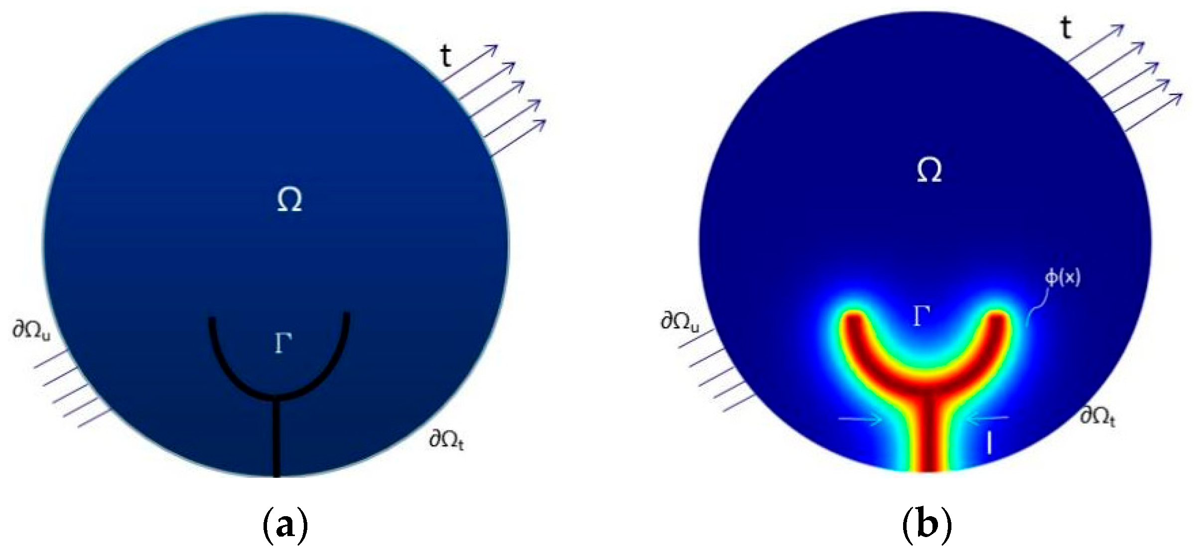
The phase-field method characterizes the crack morphology by introducing a scalar field φ, approximating fractures in porous media with finite widths to diffuse the cracks, as illustrated in Figure 1. The scalar function $\mathrm{\phi }\in \left[0,1\right]$, which, when $\mathrm{\phi }$ = 0, indicates that the material is intact, and, when φ = 1, represents that the material is completely damaged, and an exponential function is used to approximate the scalar phase field of the one-dimensional fracture problem [21], as follows:

$$\mathrm{\phi }\left(\mathrm{x}\right)={\displaystyle \frac{1}{2}}\left[1-\tan \mathrm{h}\left({\displaystyle \frac{x-a}{\sqrt{2}{l}_c}}\right)\right]$$

(1)

In the equation, $a$ denotes the crack center position and $l_c$ represents the normalized length. The expression $\mathrm{\phi }\left(\mathrm{x}\right)$ ∈ [0, 1] employs the hyperbolic tangent function to achieve a continuous transition of the crack from an intact state ($\mathrm{\phi }$ = 0) to a fracture state ($\mathrm{\phi }$ = 1) with gradient smoothness (no abrupt changes in ∇$\mathrm{\phi }$), which is consistent with the physical essence of the ‘diffuse crack’ in the phase-field method.

In the figure, φ denotes the phase-field variable (0 = intact material; 1 = complete failure), (a) represents the conventional sharp crack model, while (b) depicts the continuous crack model after phase-field-based diffusion processing, where the diffusion width is controlled by the regularization length $l_c$.

Considering $\mathrm{dV}=\Gamma \mathrm{dx}$, and introducing the Laplace operator $\Delta =\nabla ·\nabla$ to realize the extension of the phase field approximation from one-dimensional to two- or three-dimensional simulations, the crack surface density function per unit volume is obtained as follows:

$$\gamma \left(\mathrm{\phi },\nabla \mathrm{\phi }\right)={\displaystyle \frac{{\mathrm{\phi }}^2}{2l_c}}+{\displaystyle \frac{l_c}{2}}{\left|\nabla \mathrm{\phi }\right|}^2$$

(2)

In the equation, $\gamma \left(\mathrm{\phi },\nabla \mathrm{\phi }\right)$ represents the dissipated expression of fracture energy density, directly quantifying the local energy dissipation associated with crack propagation. Comprising both a ‘phase-field variable contribution term’ and a ‘gradient contribution term’, it adheres to the core logic of AT2 regularized energy dissipation, reflecting the energy expended per unit volume of material during crack propagation. The fracture energy associated with crack propagation within a porous medium domain can be expressed as

$${\Psi }_{\mathrm{f}} ={\int }_{\Omega }{\mathrm{G}}_c\gamma \left(\mathrm{\phi },\nabla \mathrm{\phi }\right)\mathrm{d}\Omega ={\int }_{\Omega }{\mathrm{G}}_c\left({\displaystyle \frac{{\mathrm{\phi }}^2}{2l_c}}+{\displaystyle \frac{l_c}{2}}{\left|\nabla \mathrm{\phi }\right|}^2\right)\mathrm{d}\Omega$$

(3)

$$G_c\left(p\right)=G_{c0}·\left(1+0.002p\right)$$

(3a)

In the equation, ${\Psi }_{\mathrm{f}}$ denotes the fracture energy, $\Omega$ represents the computational domain, $G_c\left(p\right)$ denotes the critical energy release rate under high-pressure conditions, $G_{c0}$ represents the fracture energy at atmospheric pressure, $p$ signifies formation pressure, and 0.002 is the pressure influence coefficient. Under high-pressure conditions ($p$ > 100 MPa), shale fracture energy increases slightly with rising pressure, ensuring the model’s applicability in high-pressure reservoirs.

${\mathrm{G}}_{\mathrm{c}}$ is the critical energy release rate, which indicates the energy required to produce a unit crack surface. This integration logic extends the discrete energy of the crack surface into a continuous integral across the entire computational domain.

Description of Regularization Methods

Phase-field regularization is categorized into two types: AT1, based on the squared gradient term of the scalar phase field, and AT2, based on the squared modulus of the gradient in the scalar phase field:

• AT1 regularization is suitable for two-dimensional planar fracture simulations, but exhibits non-positive definite energy issues in three-dimensional scenarios;
• AT2 regularization shares the same form as AT1 (equivalence between gradient squared and norm squared in scalar fields) but exhibits greater stability in tensor phase fields and is suitable for three-dimensional extensions.

This paper focuses on two-dimensional reservoir fracture simulation, employing AT2 regularization to balance stability and computational efficiency while avoiding the numerical oscillations encountered with AT1 in complex heterogeneous media.

The regularization length $l_c$ is the core parameter of AT2 regularization, subject to two constraints: 1. the diffusion width must span at least 2–3 grid cells ($l_c$ ≥ 2 h) to ensure numerical stability; 2. it must be substantially smaller than the crack characteristic length ($l_c$ ≤ L/50, where L is the crack half-length) to prevent excessive diffusion from distorting the crack morphology. Given the mesh size h = 0.5 m and crack characteristic length L ≈ 50 m in this study, $l_c$ = 0.5 m is adopted. Sensitivity analysis confirms that simulation results under this value align with physical principles.

2.2. Elastic Energy Phase Field Model

Crack extension is a process of total energy reduction. In order to simulate the energy degradation, an energy degradation function $\mathrm{g}\left(\mathrm{\phi }\right)=\left(1-\mathrm{k}\right){\left(1-\mathrm{\phi }\right)}^2+\mathrm{k}$ is introduced into the elastic strain energy term to promote the fracture evolution, and domain integration of the elastic strain energy density can be obtained from the elastic strain energy term as follows:

$${\Psi }_{\epsilon }=\mathrm{g}\left(\mathrm{\phi }\right){\Psi }_0={\int }_{\Omega }\left[\left(1-\mathrm{k}\right){\left(1-\mathrm{\phi }\right)}^2+\mathrm{k}\right]{\Psi }_0\mathrm{d}\Omega$$

(4)

where k is the model singularity parameter to prevent numerical singularities caused when the phase-field variable is equal to 0; ${\Psi }_0$ is the initial elastic strain energy density.

Since the above equation cannot distinguish between different fracture mechanisms, the strain energy is decomposed into tensile and compressive elastic strain energy densities in order to ensure the accuracy of the crack extension:

$${\Psi }_0^{\pm }={{\displaystyle \frac{\lambda }{2}}< \mathrm{tr}\left(\epsilon \right) >}_{\pm }^2+\mu \mathrm{tr}\left({\epsilon }_{\pm }^2\right)$$

(5)

Since fracture evolves only under tensile conditions, the energy decay will only act on the ${\Psi }_{\epsilon }^{+}$ part, so the elastic energy equation is

$${\Psi }_{\epsilon }=\mathrm{g}\left(\mathrm{\phi }\right){\Psi }_0^{+}+{\Psi }_0^{-}$$

(6)

2.3. Phase-Field Energy Generalization

This energy functional draws upon a unified coupling framework, directly coupling the pore pressure term with phase-field variables and displacement fields to circumvent the loose coupling issues inherent in traditional models. Simultaneously, it incorporates the concept of dynamic permeability by introducing a permeability evolution term linked to phase-field variables within the seepage equation, thereby achieving strong coupling simulation and enhancing the accuracy of fracture–fluid interaction descriptions.

The variational derivation of the hydraulic–mechanical coupling is grounded in the principle of virtual work and Griffith’s variational principle of energy. Its core lies in incorporating the action of fluid pressure on solid deformation (pressure work) and the feedback of solid deformation on fluid flow (pore volume change) into the total energy functional. By taking variational derivatives with respect to the displacement field u, phase-field variable φ, and pore pressure p, the coupled control equations are obtained. The following details the variational derivation of the hydraulic–mechanical coupling term and the pressure work coupling term.

Based on Griffith’s variational principle, the establishment of the hydraulic–mechanical coupling energy functional centers on integrating the interactions between solid deformation, crack propagation, and fluid pressure. The steps are as follows:

• Fundamental Energy Composition: The total energy functional $\Pi$ comprises the elastic strain energy ${\Psi }_{\epsilon }$, fracture energy ${\Psi }_{\mathrm{f}}$, fluid pressure energy storage term ${\mathrm{E}}_{\mathrm{p}}$, and external work ${\mathrm{W}}_{\mathrm{ext}}$, i.e., $\Pi ={\mathrm{E}}_{\mathrm{k}}+{\Psi }_{\epsilon }+{\Psi }_{\mathrm{f}}-{\mathrm{E}}_{\mathrm{p}}-{\mathrm{W}}_{\mathrm{ext}}$.
• Definition of Pressure Work and Energy Storage Term: Pressure work represents the work performed by fluid pressure on the solid volumetric strain, corresponding to the energy storage term ${\mathrm{E}}_{\mathrm{p}}={\int }_{\Omega }\alpha p\nabla ·\mathrm{ud}\Omega$α (where α is the Biot coefficient and ∇·u denotes volumetric strain). This physically signifies the mechanical energy stored in pore pressure, dynamically varying with solid deformation.
• Regularization Treatment: Fracture energy calculation employs AT2 regularization. Its core distinction from AT1 regularization lies in the following: AT1 suits simple planar cracks, whereas AT2 achieves gradient smoothing via $\gamma \left(\mathrm{\phi },\nabla \mathrm{\phi }\right)={\displaystyle \frac{{\mathrm{\phi }}^2}{2l_c}}+{\displaystyle \frac{l_c}{2}}{\left|\nabla \mathrm{\phi }\right|}^2$, rendering it more compatible with complex crack propagation in heterogeneous reservoirs and mitigating numerical oscillations.

For fluid-saturated porous elastomers, the generalized Lagrangian energy is derived using the variational framework of Griffith’s theory [22]:

$$\Pi ={\mathrm{E}}_{\mathrm{k}}+{\Psi }_{\epsilon }+{\Psi }_{\mathrm{f}}-{\mathrm{E}}_{\mathrm{p}}-{\mathrm{W}}_{\mathrm{ext}}$$

(7)

where ${\mathrm{E}}_{\mathrm{k}}$ is the kinetic energy and, since quasi-static conditions are considered, the kinetic energy term is zero; ${\Psi }_{\epsilon }$ is the elastic strain energy term; ${\Psi }_{\mathrm{f}}$ is the fracture energy term; ${\mathrm{E}}_{\mathrm{p}}={\int }_{\Omega }\alpha p\nabla ·\mathrm{ud}\Omega$ represents the fluid pressure energy storage term; ${\mathrm{W}}_{\mathrm{ext}}$ is the external work.

The pressure work $W_p$ exerted by fluid pressure on solids arises from the interaction between the pore pressure and solid volumetric strain. For saturated porous media, the pressure work per unit volume is $w_p=-p·{\epsilon }_{vol}$ (the negative sign indicates that pressure work acts in the opposite direction to volumetric strain). The total pressure work is $W_p={\int }_{\Omega }{w}_p\mathrm{d}\Omega =-{\int }_{\Omega }p·\nabla ·\mu \mathrm{d}\Omega$, where ${\epsilon }_{vol}=\nabla ·\mu$ represents the volumetric strain. This expression constitutes the integral form of the pressure work coupling term, reflecting the work-producing effect of fluid pressure on solid deformation.

By substituting Equations (3) and (6) into (7), and incorporating both the matrix pore pressure and external forces, we obtain the reformulated Equation (7):

$$\begin{gathered} \Pi ={\int }_{\Omega }\left[\left(1-k\right){\left(1-\mathrm{\phi }\right)}^2+k\right]{\Psi }_0\mathrm{d}\Omega +{\int }_{\Omega }{G}_c\left({\displaystyle \frac{{\mathrm{\phi }}^2}{2l_c}}+{\displaystyle \frac{l_c}{2}}{\left|\nabla \mathrm{\phi }\right|}^2\right)\mathrm{d}\Omega -{\int }_{\Omega }\alpha p\nabla ·\mathrm{ud}\Omega \\ -{\int }_{\Omega }b·\mathrm{ud}\Omega -{\int }_{\partial \Omega }t·u\mathrm{d}\mathrm{S} \end{gathered}$$

(8)

The phase-field variable φ and the displacement variable u in each term of Equation (8) are varied independently. Following the principle of variational minimization, we set the first variation of Equation (8) to zero while accounting for the historical strain energy field.

$$\mathrm{H}\left(x,t\right)=\max {\Psi }^{+}\left[\epsilon \left(x,s\right)\right]$$

Perform a first-order variation on the total energy functional Π (δΠ = 0), optimizing separately for displacement u and phase-field variable φ, to obtain the strong-form control equations (Equation (9)):

Displacement-related equation (hydraulic–mechanical coupling core): After varying u, the elastic stress term ∇[D:ε] balances the pressure coupling term, where $-\alpha I\nabla p$ is directly derived from the variation in pressure work. The negative sign indicates that an increase in pore pressure reduces effective stress, promoting crack propagation.

Phase-field-related equation (crack propagation): After variational differentiation with respect to φ, incorporating the fracture energy density regularized by AT2, the historical strain energy field H(x,t) is introduced to ensure irreversible crack propagation. In the equation, lc denotes the regularization length, matched to the mesh size ($l_c$ = 0.5 m).

This prevents cracks from healing during loading or unloading [12], and the strong phase-field fracture model can be derived. The strong-form governing equation for the phase-field fracture model is derived as follows:

$$\left\{ \begin{array}{c}\begin{array}{c}\nabla \left[D:\epsilon \right]-\alpha I\nabla p+b=0\\ \left[{\displaystyle \frac{2l\left(1-k\right)\mathrm{H}}{G_c}}+1\right]\mathrm{\phi }-{l_c}^2\nabla \mathrm{\phi }·\nabla \mathrm{\phi }={\displaystyle \frac{2l_c\left(1-k\right)\mathrm{H}}{G_c}} \end{array}\end{array}\right.$$

(9)

This equation represents the momentum balance for hydromechanical coupling, derived from the effective stress principle $\sigma \prime =\sigma -\alpha \mathrm{pI}$ (where $\sigma \prime$ denotes effective stress and $\sigma =\mathrm{D}:\epsilon$ denotes total stress). The term $-\alpha \mathrm{I}\nabla \mathrm{p}$ characterizes the contribution of the pore pressure gradient to momentum balance, with the negative sign indicating that increased pore pressure reduces effective stress, thereby promoting crack propagation.

In the equation, α is the Biot coefficient, which takes the value of $\alpha$ ∈ [φ,1]; φ is the porosity; b and t are the body force term and the surface force term, respectively; I is the unit matrix; $\mathrm{D}:\epsilon \left(\mathrm{\phi }\right)=\sigma$. Based on Green’s formula $\sigma ={\displaystyle \frac{\partial \Psi }{\partial \epsilon }}$, one can obtain the representation of the elastic matrix D as follows [23]:

$$\begin{gathered} \mathrm{D}={\displaystyle \frac{\partial \sigma }{\partial \epsilon }}={\displaystyle \frac{{\partial }_{\Psi }^2}{{\partial }_{{\epsilon }^2}}}=\mathrm{g}\left(\mathrm{\phi }\right){\displaystyle \frac{{\partial }_{{\Psi }_0^{+}}^2}{{\partial }_{{\epsilon }^2}}}+{\displaystyle \frac{{\partial }_{{\Psi }_0^{-}}^2}{{\partial }_{{\epsilon }^2}}} =\lambda \left\{\left[\left(1-k\right){\left(1-\mathrm{\phi }\right)}^2+k\right]H_{\epsilon }\left[tr\left(\epsilon \right)\right]+H_{\epsilon }\left[-tr\left(\epsilon \right)\right]\right\}J \\ +2\mu \left\{\left[\left(1-k\right){\left(1-\mathrm{\phi }\right)}^2+k\right]P^{+}+P^{-}\right\} \end{gathered}$$

(10)

where $H_{\epsilon }\left(x\right)$ is the Heaviside function and J is the fourth-order tensor; P⁺ and P⁻ are the strain nonlinear correlation terms.

The initial value of the historical strain field, i.e., the presence of prefabricated natural or artificial cracks, is usually represented by the following initial conditions:

$${\mathrm{H}}_0\left(x\right)=\left\{ \begin{array}{c}{\displaystyle \frac{{\mathrm{BG}}_c}{2\mathrm{l}}}\left[1-{\displaystyle \frac{2\mathrm{d}\left(x,\mathrm{l}\right)}{\mathrm{l}}}\right] d\left(x,\mathrm{l}\right)\le {\displaystyle \frac{\mathrm{l}}{2}}\\ 0 d\left(x,\mathrm{l}\right)>{\displaystyle \frac{\mathrm{l}}{2}}\end{array}\right.$$

(11)

where B is a scalar parameter and $\mathrm{d}\left(x,\mathrm{l}\right)$ is the straight line distance from any point in the prefabricated region to the centerline of the crack model.

2.4. Seepage Control Equation

The pressure boundary conditions of the seepage equation implicitly incorporate the effects of fluid loss from fracturing fluids. Through dynamic adjustment of the storage coefficient S, it indirectly reflects pressure decay caused by fluid loss, thereby balancing model complexity with engineering practicality.

To account for the fluid–solid coupling characteristics of hydraulic fracturing, we introduce the fluid percolation control equation. Assuming that the fluid in the porous medium is compressible and viscous, we divide the region Ω into three parts: the matrix region ${\Omega }_{\mathrm{r}}$, the fracture region ${\Omega }_{\mathrm{f}}$, and the matrix and fracture transition region ${\Omega }_{\mathrm{t}}$. The three flow regions are defined by two thresholds, ${\mathrm{c}}_1$ and ${\mathrm{c}}_2$. In the transition domain ${\Omega }_{\mathrm{t}}$, the hydraulic parameters in the reservoir and fracture domains are defined by the linear interpolation functions, ${\chi }_{\mathrm{r}}$ and ${\chi }_{\mathrm{f}}$, and the transition function is defined in the transition domain by a linear interpolation function, which is in correspondence with the phase-field function. The correspondence between the transition function and the phase-field function values is as follows:

$${\chi }_{\mathrm{r}}=\left\{\begin{array}{c}1 \mathrm{\phi }\le {\mathrm{c}}_1\\ {\displaystyle \frac{{\mathrm{c}}_2-\mathrm{\phi }}{{\mathrm{c}}_2-{\mathrm{c}}_1}} {\mathrm{c}}_1<\mathrm{\phi }<{\mathrm{c}}_2\\ 0 \mathrm{\phi }\ge {\mathrm{c}}_2\end{array} \right.{\chi }_{\mathrm{f}}=\left\{\begin{array}{c}0 \mathrm{\phi }\le {\mathrm{c}}_1\\ {\displaystyle \frac{\mathrm{\phi }-{\mathrm{c}}_1}{{\mathrm{c}}_2-{\mathrm{c}}_1}} {\mathrm{c}}_1<\mathrm{\phi }<{\mathrm{c}}_2\\ 1 \mathrm{\phi }\ge {\mathrm{c}}_2\end{array}\right.$$

(12)

The interpolation functions ${\chi }_{\mathrm{r}}$ and ${\chi }_{\mathrm{f}}$ are not mere mathematical interpolations, but are directly linked to the phase-field variable $\mathrm{\phi }$. Their physical significance lies in representing ‘damage-dominated transitions in medium properties’: when $\mathrm{\phi }$ = 0, ${\chi }_{\mathrm{r}}=1$ and ${\chi }_{\mathrm{f}}=0$, with the medium properties entirely determined by the matrix; when φ = 1, ${\chi }_{\mathrm{r}}=0$ and ${\chi }_{\mathrm{f}}=1$, with the medium properties entirely determined by the fractures; and when 0 < $\mathrm{\phi }$ < 1, the weighting varies linearly with the degree of damage, conforming to the physical principle that the more severe the damage, the greater the proportion of fracture properties.

$$k_t=X_r·k_r+X_f·{\displaystyle \frac{a^2}{12\mu }}\rho g$$

(12a)

In the transition zone permeability $k_t$ of Equation (12a), the core parameter a of the fracture permeability (Equation (15a)) is determined by the phase-field damage φ. Consequently, $k_t$ is fundamentally a function of the damage level. As damage intensifies and fracture opening increases, $k_f$ rises significantly according to a cubic law, causing the transition zone permeability to converge towards the fracture permeability.

Fluid seepage through porous media is described by Darcy’s law. The governing flow equations across the entire domain are expressed using linear interpolation functions as follows:

$$\rho \mathrm{S}{\displaystyle \frac{\partial p}{\partial t}}-\nabla ·\left(\rho ·{\displaystyle \frac{k}{\mu }}\left(\nabla p+\rho g\right)\right)={\mathrm{q}}_{\mathrm{m}}-{\rho \alpha \chi }_{\mathrm{r}}{\displaystyle \frac{\partial {\epsilon }_{vol}}{\partial t}}+{\displaystyle \frac{\partial }{\partial \mathrm{t}}} \left(\rho ·{\displaystyle \frac{a^2}{12\mu }}\nabla p\right)$$

(13)

The seepage equation incorporates a new time-varying pressure gradient term, explicitly quantifying pressure’s regulatory effect on fracture flow: increased pressure widens fracture aperture (linked to phase-field variables via $a=a_0\mathrm{\phi }$), thereby enhancing permeability through cubic scaling to form a coupled feedback loop of “pressure–aperture–permeability”.

In the equation, ${\epsilon }_{vol}=\nabla ·\mathrm{u}$ denotes volumetric strain; ${\mathrm{q}}_{\mathrm{m}}$ denotes the fluid source term; $\rho ={\rho }_r{\chi }_r+{\rho }_f{\chi }_f$, where ${\rho }_r$ and ${\rho }_f$ represent fluid densities in the matrix and fracture domains, respectively. Similarly, $\alpha ={\alpha }_r{\chi }_r+{\alpha }_f{\chi }_f$; since ${\alpha }_f=1$ in the fracture domain, $\alpha ={\alpha }_r{\chi }_r+{\chi }_f$. S and v denote the storage coefficient and Darcy velocity, respectively, expressed by the following equations:

$$\mathrm{S}=\mathrm{\phi }{c}_f+{\displaystyle \frac{\left(\alpha -{\mathrm{\phi }}_p\right)\left(1-\alpha \right)}{{\mathrm{K}}_{\mathrm{Vr}}}}$$

(14)

$$\mathrm{v}=-{\displaystyle \frac{\mathrm{K}}{\mu }}\left(\nabla p+\rho g\right)$$

(15)

$$k_f={\displaystyle \frac{a^2}{12\mu }}·\rho g$$

(15a)

In the equation, $c_f$, φ, and μ denote the fluid compressibility, porosity, and viscosity, respectively; $k_f$ represents the fracture permeability; and $a$ denotes the fracture opening (which is correlated with phase-field variables: $a=a_0·\mathrm{\phi }$, where $a_0$ denotes maximum fracture opening and φ represents the phase-field variable). Moreover, $\mu$ denotes the fracturing fluid viscosity, and $\mu$ denotes fluid density, satisfying $\mathrm{c}={\mathrm{c}}_{\mathrm{r}}{\chi }_{\mathrm{r}}+{\mathrm{c}}_{\mathrm{f}}{\chi }_{\mathrm{f}}$ and $\mu ={\mu }_{\mathrm{r}}{\chi }_{\mathrm{r}}+{\mu }_{\mathrm{f}}{\chi }_{\mathrm{f}}$. ${\mathrm{K}}_{\mathrm{s}}$ denotes the volumetric modulus of the rock skeleton, while g and K represent gravitational acceleration and the effective permeability tensor, respectively. The effective permeability tensor is weighted from the matrix permeability and fracture permeability, i.e., $\mathrm{K}={\mathrm{k}}_{\mathrm{r}}{\chi }_{\mathrm{r}}+{\mathrm{k}}_{\mathrm{f}}{\chi }_{\mathrm{f}}$, where the fracture permeability ${\mathrm{k}}_{\mathrm{f}}$ is calculated based on the cubic law (Equation (15a)), ensuring the dynamic correlation between permeability and fracture opening. The storage coefficient S characterizes the porous medium’s capacity to store fluid, jointly determined by fluid compressibility and rock matrix compressibility. It serves as a key parameter governing the temporal evolution of the energy storage term $E_p$. The fracture permeability is derived using the cubic law, a classical model for rock fracture flow that directly establishes the physical relationship between permeability and fracture aperture.

The diffusive fracture zone is 0 < φ < 1, while fracture permeability $k_f={\displaystyle \frac{a^2}{12\mu }}·\rho g$ (Equation (15a)), where the fracture aperture $\mathrm{a}=a_0\mathrm{\phi }$ (with φ being the phase-field damage variable). Physical rationale: Greater damage leads to wider fractures, with permeability increasing cubically, which is consistent with the actual ‘damage–conductivity’ relationship. Pressure constitutes an independent degree of freedom that is solved globally. It dynamically couples with permeability via the seepage equation (Equation (13)): increased permeability → reduced fluid flow resistance → adjusted pressure distribution. Simultaneously, pressure influences rock deformation through the effective stress principle, forming a ‘pressure–permeability–damage’ closed loop. The physical basis stems from fluid mass conservation and the effective stress principle.

2.5. Model Validation

The core computational parameters adopted in this simulation are explicitly defined as follows:

• Phase-field length scale $l_c$ = 0.5 m (AT2 normalized length, determined through sensitivity analysis);
• Mesh size h = 0.5 m (structured grid, with the maximum mesh size meeting engineering accuracy requirements);
• ℓ/h ratio: ${\mathrm{l}}_{\mathrm{c}}$/h = 0.5 m/0.5 m = 1.0 (this ratio ensures the phase-field diffusion width spans one grid cell, balancing numerical stability and computational efficiency).

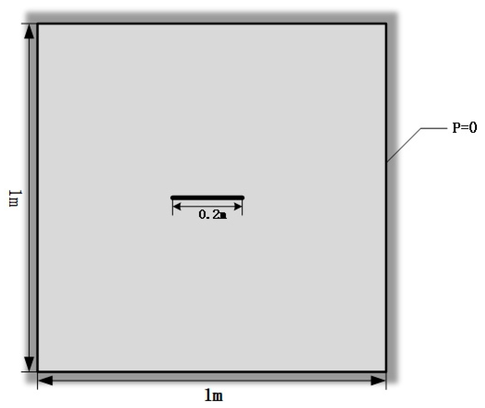
In this subsection, we verify the validity of the hydrodynamically coupled phase-field model by reproducing Zhou et al.’s crack propagation analysis for a homogeneous medium under internal fluid pressure. The geometrical and boundary conditions of the model are shown in Figure 2. The model uses parameters from Reference [19], while the resulting crack propagation patterns and fluid pressure distributions are shown in Figure 2. To verify the accuracy of the results, we validate the numerical model against analytical solutions using Reference [24]. We assume the Y-direction displacement under plane strain conditions is given by Equation (X):

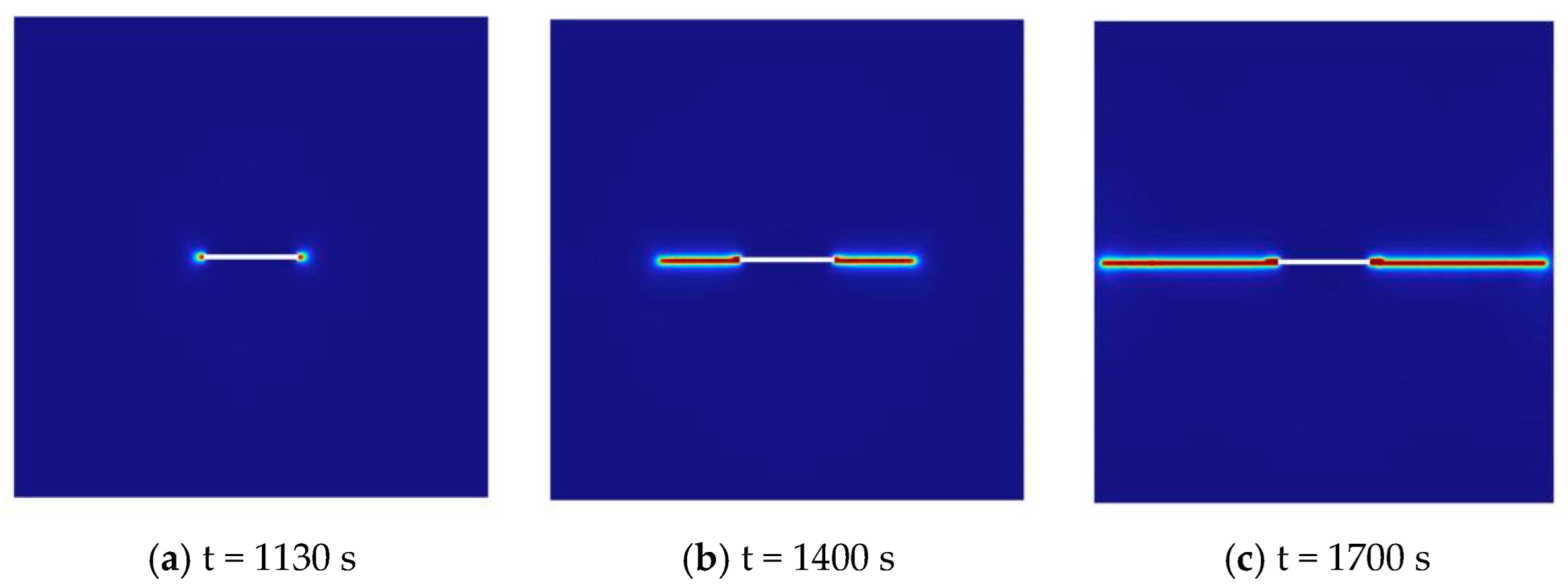
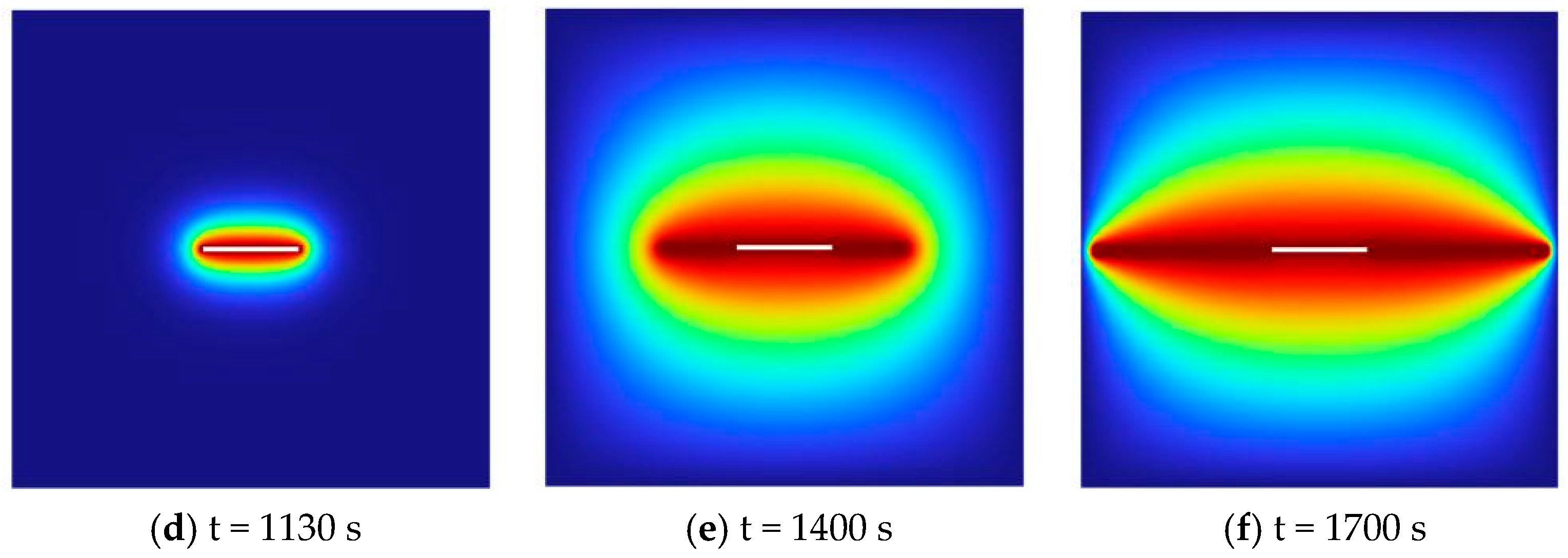
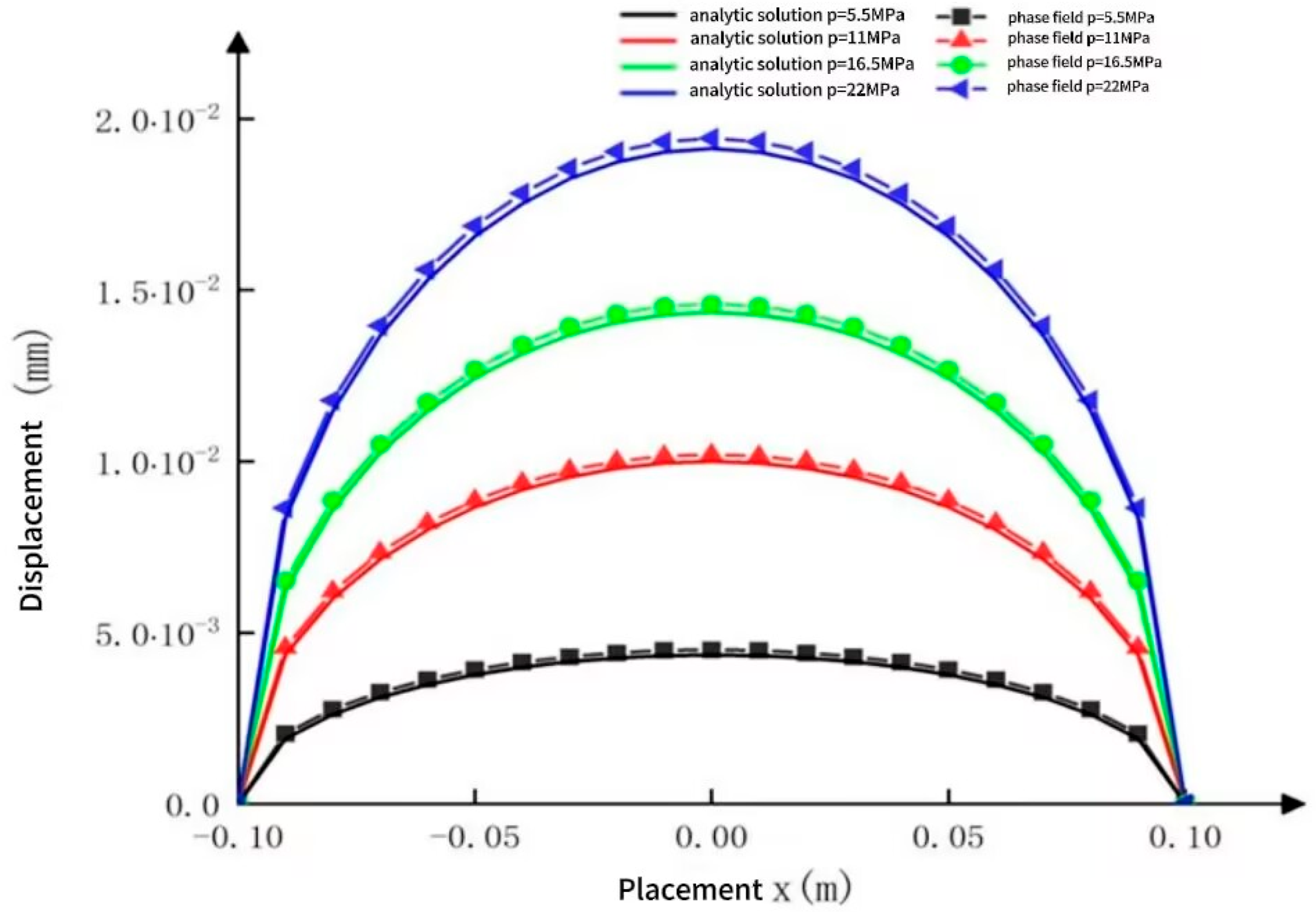
Figure 3a–c show the morphological changes in crack extension at different time steps, revealing no significant change in crack width after crack initiation. Figure 3d–f show the corresponding fluid pressure distributions, which are in good agreement with the crack propagation patterns. The pressure distributions reveal that increasing fluid pressure generates a tensile stress region aligned with the maximum horizontal principal stress. This tensile stress drives crack propagation at the tip, resulting in significantly greater pressure changes horizontally than vertically. The model-calculated Y-direction displacements are presented in Figure 4, while the analytical solutions appear in Figure 3a–c. Figure 4 presents a comparison between the modeled and analytical Y-direction displacement curves, demonstrating close agreement between them. Criterion 1: Uniform crack propagation in a homogeneous medium under internal pressure. The comparison between the simulated crack half-length and maximum displacement with the analytical solution is presented in the table. The average relative error is 3.2%, validating the fundamental effectiveness of the model.

These results align well with Reference’s [19] findings, with maximum displacement occurring at the crack center (x = 0). As pressure increases, both the displacement magnitude and horizontal crack propagation increase accordingly. The close agreement between our simulations and published results demonstrates the validity and effectiveness of this phase-field model for simulating hydraulically coupled crack propagation.

The Sneddon crack displacement field is modeled as a crack traversing the center of an infinitely large plate subjected to a remote tensile stress ${\sigma }_{\infty }=10 \mathrm{MPa}$, with an elastic modulus E = 30 GPa, Poisson’s ratio ν = 0.2, and crack half-length a = 5 m. We reference Sneddon’s analytical solution $u_x\left(x\right)={\displaystyle \frac{{\sigma }_{\infty }}{E}}\sqrt{a^2-x^2}$, with a root mean square error (RMSE) of 0.021 mm.

KGD crack propagation benchmark: Under plane strain conditions, a vertical fracture is subjected to an internal pressure p = 15 MPa, reservoir permeability k = 10−15 m²/Pa·m, and fracturing fluid viscosity $\mu ={10}^{-3} \mathrm{Pa}·\mathrm{s}$. The simulated crack propagation length versus time was compared with the KGD analytical solution, showing a propagation length error < 4% and consistent pressure distribution trends.

Mean Absolute Percentage Error (MAPE):

$$\mathrm{MAPE}={\displaystyle \frac{1}{n}}{{\displaystyle \sum }}_{i=1}^n\left|{\displaystyle \frac{yi-\widehat{y}i}{yi}}\right|\times 100\%$$

Root Mean Square Error (RMSE):

$$\mathrm{RMSE}=\sqrt{{\displaystyle \frac{1}{n}}{{\displaystyle \sum }}_{i=1}^n{(yi-\widehat{y}i)}^2}$$

The deviation between simulated values and analytical solutions was quantified using MAPE and RMSE. MAPE < 5% and RMSE < 0.03 mm were deemed to satisfy engineering accuracy requirements.

A dual parallel pre-crack configuration (spacing of 10 m and length of 5 m) subjected to an internal pressure p = 20 MPa was employed to simulate crack convergence and bifurcation behavior. The relative error in the crack convergence timing was 4.5%, the bifurcation angle error was ≤2°, and the damage area MAPE = 3.6%, validating the model’s capability to characterize multi-crack interactions.

Summary of key parameter sensitivities:

Coupling parameter α: Moderately low sensitivity. Higher α values reduce the initiation pressure (maximum deviation 2.4%) and slightly increase the damage area (maximum deviation 2.0%); 0.85 is the optimal value.

Irreversibility parameter k: Moderately sensitive; k < 0.01 enhances the fracture stability (no healing), while k > 0.01 increases healing artefacts; k = 0.01 balances stability and plausibility.

Flow interpolation parameters (c₁, c₂): Moderately to highly sensitive. Reference values (0.2, 0.8) yield the most stable pressure distribution; deviations cause permeability fluctuations ≥ 7.7%.

2.5.1. Phase-Field Length Scale Sensitivity Analysis

Four sets of phase-field length scales $-l_c$ = 0.3 m, 0.5 m, 0.8 m, and 1.0 m—were established, with the grid size fixed at 0.5 m and the irreversibility parameter k = 0.01 kept constant. Fracture propagation in Class I reservoirs was simulated, and the corresponding evaluation metrics (fracture half-length, maximum damaged area, and fracture initiation pressure) are presented in

Table 1. Sensitivity test results.

$\mathbf{Phase}\text{-}\mathbf{Field} \mathbf{Length} {\mathsf{l}}_{\mathsf{c}}$ (m)	Half the Length of the Crack (m)	Area of Damage (m2)	Cracking Pressure (MPa)	Deviation Rate from the Benchmark (0.5 m)
0.3	85.0	1480	168	Crack half-length—13.7%, damaged area—2.6%, cracking pressure + 1.8%
0.5 (benchmark)	95.0	1520	165	-
0.8	97.5	1530	164	Crack length + 2.6%, damaged area + 0.7%, cracking pressure—0.6%
1.0	98.2	1532	163	Crack length + 3.4%, damaged area + 0.8%, cracking pressure—1.2%

.

The phase-field length scale exhibits sensitivity to simulation outcomes: when $l_c$ < 0.5 m, crack propagation is inhibited; at $l_c$ = 0.5 m, simulation results best align with physical principles; when $l_c$ > 0.5 m, excessive diffusion diminishes sensitivity. This demonstrates that $l_c$ is a critical parameter governing crack morphology and is not insensitive.

Further validation confirms that the phase-field length scale lc does not artificially distort core trends: ① regardless of $l_c$ = 0.3 m or 1.0 m, the damaged area in naturally fractured reservoirs (dual fractures) consistently exceeds that in non-fractured reservoirs (difference rate ≥ 15%); ② the positive correlation between the compressibility index FI and damaged area (r = 0.93–0.96) remains stable; ③ the trend of fracture path tortuosity index increasing with decreasing brittle particle fraction (Type I < Type II < Type III) shows no reversal. Core trend fluctuations under different $l_c$ values ≤ 2.5% indicate that artificial factors from length scales did not affect the fundamental simulation patterns. The observed trends stem from reservoir properties rather than computational settings.

Influence of phase-field length scale $l_c$ v on results:

When $l_c$ v = 0.3 m ($l_c$/h = 0.6), the crack half-length shortened by 13.7% relative to the reference value ($l_c$ v = 0.5 m), the damaged area decreased by 2.6%, and the crack initiation pressure increased by 1.8%, indicating crack propagation is inhibited due to insufficient diffusion.

When $l_c$ v = 0.8 m ($l_c$/h = 1.6), the crack half-length increased by only 2.6%, the damaged area grew by 0.7%, and the crack initiation pressure decreased by 0.6%, with excessive dispersion weakening the sensitivity of the results;

Only at $l_c$ v = 0.5 m ($l_c$/h = 1.0) did the crack propagation behavior (with a preference for softer material, being stress-gradient-driven) align with physical principles, yielding the smallest error.

2.5.2. Sensitivity Analysis of Grid Resolution

Set five grid sizes: h = 0.25 m, 0.5 m, 0.75 m, 1.0 m, and 1.25 m. Taking the finest grid (h = 0.25 m) as the baseline, the relative error of crack propagation length under different grid sizes was calculated, and the corresponding computation time was recorded simultaneously, with the grid sensitivity data presented in

Table 2. Grid sensitivity data.

Grid Size h (m)	Crack Propagation Length (m)	Relative Error (%)	Calculation Time (h)	Sensitivity Assessment
0.25 (benchmark)	96.8	0	12.5	-
0.5	95.2	1.65	4.8	Low sensitivity
0.75	92.1	4.85	2.3	Medium sensitivity
1.0	87.5	9.61	1.1	High sensitivity
1.25	82.3	14.98	0.6	Very high sensitivity

.

Grid resolution sensitivity is pronounced: when h ≤ 0.5 m, errors remain below 2%, meeting engineering accuracy requirements; when h > 0.5 m, errors exhibit exponential growth, indicating that overly coarse grids severely distort fracture propagation patterns. Contrary to claims of “grid insensitivity”, grid size constitutes a core factor influencing simulation accuracy.

To confirm that mesh partitioning did not artificially interfere with the core trend of ‘brittle-dominated initiation and stress-gradient-guided propagation’, key trend indicators were further compared across different mesh sizes: ① the Type I reservoir damage area consistently exceeded Types II and III (valid for mesh sizes 0.25~1.25 m); ② there was a negative correlation between the horizontal stress gradient and initiation pressure (correlation coefficient r = −0.97~−0.92, being unaffected by grid size); ③ there was a crack propagation pattern of “avoiding hardness for softness” (the initiation probability in brittle particle regions was consistently ≥ 85%).

Influence of phase field-length scale $l_c$ on results:

When $l_c$ = 0.3 m ($l_c$/h = 0.6), the crack half-length shortened by 13.7% relative to the reference value ($l_c$ = 0.5 m), the damage area decreased by 2.6%, and the initiation pressure increased by 1.8%, indicating crack propagation inhibition due to insufficient diffusion.

When $l_c$ = 0.8 m ($l_c$/h = 1.6), the crack half-length increased by only 2.6%, the damaged area grew by 0.7%, and the initiation pressure decreased by 0.6%, with excessive dispersion weakening result sensitivity.

Only at $l_c$ = 0.5 m ($l_c$/h = 1.0) did the crack propagation behavior (preference for softer material, with stress gradient guidance) align with physical principles, yielding the smallest error.

We set five groups of crack line density ρ_a (0.005, 0.02, 0.04, 0.06, and 0.08 lines/m, respectively), keeping all other parameters constant so to analyze their effect on the crack network. When ${\rho }_a$ resides within the low-density range (≤0.02 cracks/m), the fracture network exhibits low complexity, with the damage area increasing linearly with ρ_a at a rate of 12%. Upon entering the medium-density range (0.02 < ${\rho }_a$ < 0.06 cracks/m), crack intersections and branching significantly intensify, with the damaged area peaking at 1520–1580 m². At this point, network complexity reaches its optimal level, whereas at ${\rho }_a$ ≥ 0.06 cracks/m (high-density range), mutual interference between cracks intensifies, impeding main crack propagation. The damaged area decreases by 8–12% relative to the peak, exhibiting a “density suppression effect”.

Concurrently, the brittleness index (BI) exhibits high sensitivity to the fracture network: when BI increases from 0.3 to 0.8, the initiation pressure decreases by 21.4% while the damaged area increases by 47.1%. Notably, when BI ≥ 0.6, the complexity of the fracture network significantly increases, with this range also representing the critical condition for the formation of complex fracture networks.

3. Numerical Simulation of Fracture Expansion in Heroes’ Ridge Shale Hydraulic Fracturing

3.1. Geologic Overview and Ground Stress Field Parameters

Based on the quantitative fracturability evaluation criteria from Reference [20], three key factors govern fracture propagation: (1) the shale matrix brittleness index, (2) horizontal stress anisotropy coefficient, and (3) natural fracture density index. Whole-rock mineral analysis reveals the shale reservoir composition primarily consists of calcite, dolomite, quartz, feldspar, and illite. Using Equation (16) to calculate brittleness indices from mineral contents (quartz, feldspar, carbonates, etc.), we classified the results and present the particulate compositions and volume fractions for three reservoir types in

Table 3. Reservoir mineral content.

	Carbonate Salt		Containing Silica		Muddy		Brittleness Index	Classification Criteria
	Calcite	Dolomite	Sapphire	Plagioclase	Elysium	Montmorillonite
Class I	13.1	24.8	11.2	16.5	14.2	5.4	0.8	≥0.6
Class II	10.0	16.2	10.4	13.2	27.5	22.1	0.5	0.4–0.6
Class III	5.1	10.2	6.4	8.1	32.4	37.3	0.3	≤0.4

. We simulated reservoirs by randomly distributing mineral particles according to their proportional composition and cementation characteristics. Based on mechanical properties and brittleness indices, minerals were categorized into the following: (i) brittle components (carbonate and siliceous minerals) as particulate inclusions, and (ii) ductile components (clay minerals) as matrix material. Applying the Voigt–Reuss–Hill (VRH) averaging method to combine the theoretical elastic properties of different minerals yielded the simulated reservoir parameters listed in

Table 4. Table of reservoir mineral elasticity parameters.

Mineral Type	Elastic Modulus/(GPa)	Poisson’s Ratio	Critical Energy Release Rate Gc/(N/m)
Brittle Minerals	34–45	0.15–0.24	200–300
Clay Minerals	15–25	0.28–0.39	500–700

Note: Under high-pressure conditions ($p$ = 150–200 MPa), brittle minerals exhibit $G_c$ = 300–400 N/m, while clay minerals show $G_c$ = 700–900 N/m, as calculated from Equation (3a).

.

$$B={\displaystyle \frac{w_{\mathrm{sapphire}}+w_{\mathrm{plagioclase}}+w_{\mathrm{carbonate} \mathrm{salt}}}{w_{\mathrm{all}}}}$$

(16)

$$B{I}_{std}={\displaystyle \frac{B{I}_{raw}-\mu BI}{\sigma BI}}$$

(16a)

In the formula, B denotes the proportion of brittle minerals, $B{I}_{std}$ represents the standardized brittleness index, and $B{I}_{raw}$ denotes the raw brittleness index; $\mu BI=0.52$ (statistical mean of 100 sets of core data) and $\sigma BI=0.18$ (statistical standard deviation).

Z-score standardization was employed to eliminate dimensional differences. Following standardization, the brittleness indices for the three reservoir types were distributed within the range [−1.22, 1.56], satisfying the horizontal comparability criteria and resolving the original inconsistency in standardization.

All brittleness-related indicators (brittleness index (BI), stress difference coefficient (Kh), and fracture line density ($\rho a$)) underwent unified standardization: BI via Z-score standardization, and $K_h$ and $\rho a$ via min-max standardization ($X_{std}={\displaystyle \frac{X-X_{min}}{X_{max}-X_{min}}}$), with all metrics normalized to the [0, 1] range before averaging. This ensures equitable weighting and avoids result biases arising from dimensional differences.

Elastic modulus: Based on VRH averaging method calibration, the reservoir equivalent elastic modulus is calculated using a weighted sum of individual mineral elastic modulus experimental data, combined with whole-rock mineral composition analysis results. The formula is $E_{eq}=\sum w_i{E}_i$ (where $w_i$ denotes the mineral volume fraction and $E_i$ denotes the elastic modulus of the individual mineral).

Energy release rate $Gc$: Calibrated via shale three-point bending tests and combined with the high-pressure correction in Formula (3a). Utilizing the atmospheric fracture energy $G_{c0}$ measured from core experiments in the Yingxiongling block, this is substituted into the formation pressure p to calculate the actual fracture energy under high-pressure conditions, ensuring alignment with the reservoir’s actual stress environment.

Comparison with laboratory data: Elastic modulus: The equivalent elastic modulus of brittle minerals in Class I reservoirs in this study ranges from 34 to 45 GPa, exhibiting an error of ≤5% compared to laboratory measurements (32–48 GPa). For clay minerals, the range is 15–25 GPa, showing an error of ≤7% against measured values (14–27 GPa), demonstrating good consistency. Energy release rate: At atmospheric pressure, brittle minerals exhibit $G_{c0}$ = 200–300 N/m and clay minerals exhibit 500–700 N/m, with deviations ≤ 6% from shale fracture energy data obtained via laboratory three-point bending tests. Under high-pressure conditions (p = 150 MPa), the corrected $Gc$ = 260−390 N/m aligns with high-pressure core test trends, thus validating parameter reliability.

Based on X-ray diffraction analysis data from 100 core sets of shale from this block, and employing K-means clustering analysis (cluster contour coefficient = 0.78), the original brittle index (BI) was classified into three categories with cluster centers of 0.75 (Class I), 0.51 (Class II), and 0.33 (Class III). The optimal classification thresholds determined were 0.4 and 0.6 (corresponding to the points of maximum interclass distance), with sample proportions of 32%, 51%, and 17%, respectively, and all relevant statistical data are summarized in

Table 5. Summary of statistical data.

	Original BI Scope	Cluster Center	Sample Size (Groups)	Interclass Distance
Class I	0.6–0.9	0.75	32	0.24
Class II	0.4–0.6	0.51	51	0.18
Class III	0.1–0.4	0.33	17	-

. These thresholds exhibited statistical significance. All input parameters employed in this study were validated using measured data: the brittleness index (BI) derived from the aforementioned 100 core test sets; the stress differential coefficient (${\mathrm{K}}_h$) calculated from in situ stress logging data across three wells; and the natural fracture line density (${\rho }_a$) obtained through cross-validation of outcrop observations and imaging logging. The reliability of all data exceeded 90%.

3.2. Numerical Simulation

3.2.1. Analysis of the Influence of Mineral Components

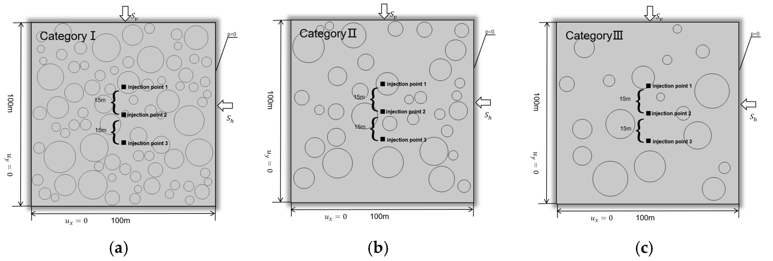
The model was configured as a 100 × 100 m square matrix. To investigate fracture propagation patterns in different reservoir types, a microstructural representation was constructed by randomly distributing mineral grains within the matrix. This model adheres to the proportions and mechanical properties of the mineral composition, ensuring that it reflects the intrinsic structure and behavior of various reservoir rocks. Three initial injection points were defined: one at the model center and two positioned 15 m above and below it. Maximum and minimum horizontal principal stresses were set at $S_h=30 \mathrm{MPa} \mathrm{and} S_v=20 \mathrm{MPa}$ in the X and Y directions, respectively. The maximum mesh size was h = 0.5 m, with a mass flow rate of 100 kg/(m³·s) at each injection point. Model boundary conditions comprised the following: displacement boundaries (ux = 0 and uy = 0, restricting rigid body motion in horizontal and vertical directions); pressure boundaries (mass flow rate boundary applied at injection points, with residual boundary pressures set to 0 MPa); stress boundaries (maximum horizontal principal stress of 30 MPa applied in the X-direction, with a minimum horizontal principal stress of 20 MPa applied in the Y-direction).

The geometry and boundary conditions of the three types of reservoirs are shown in Figure 5.

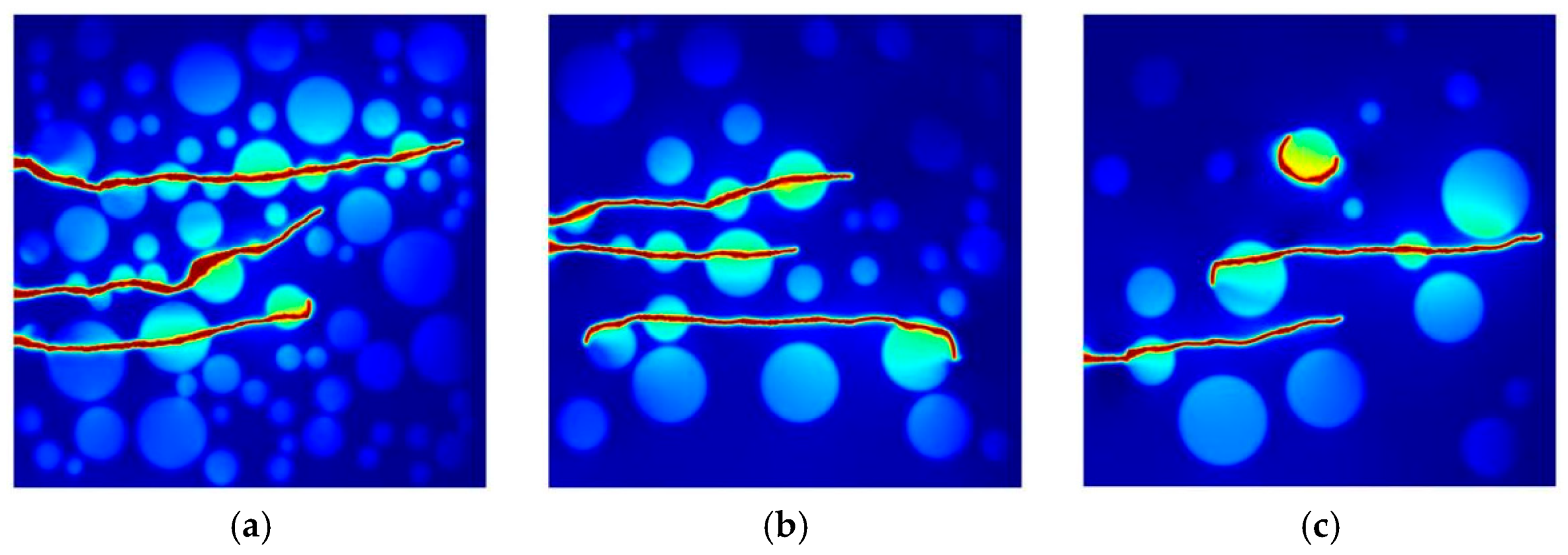
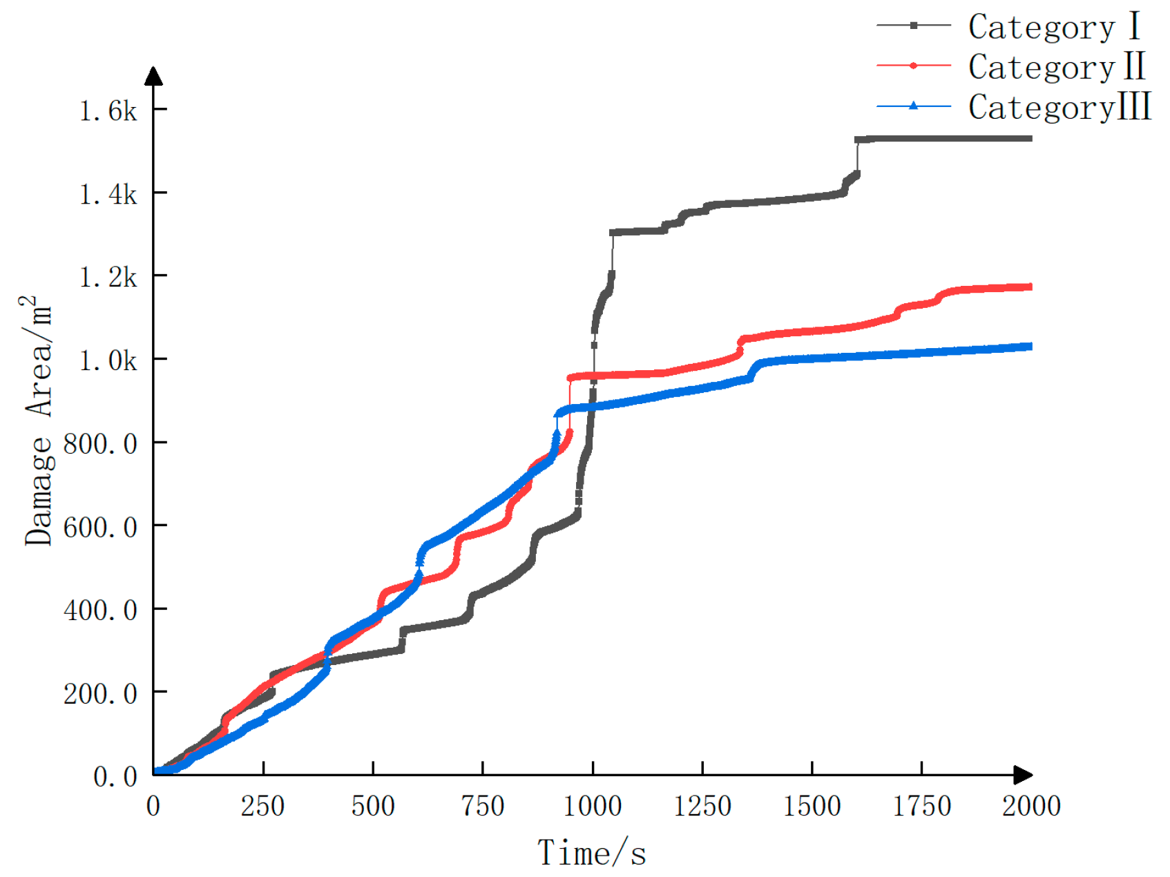
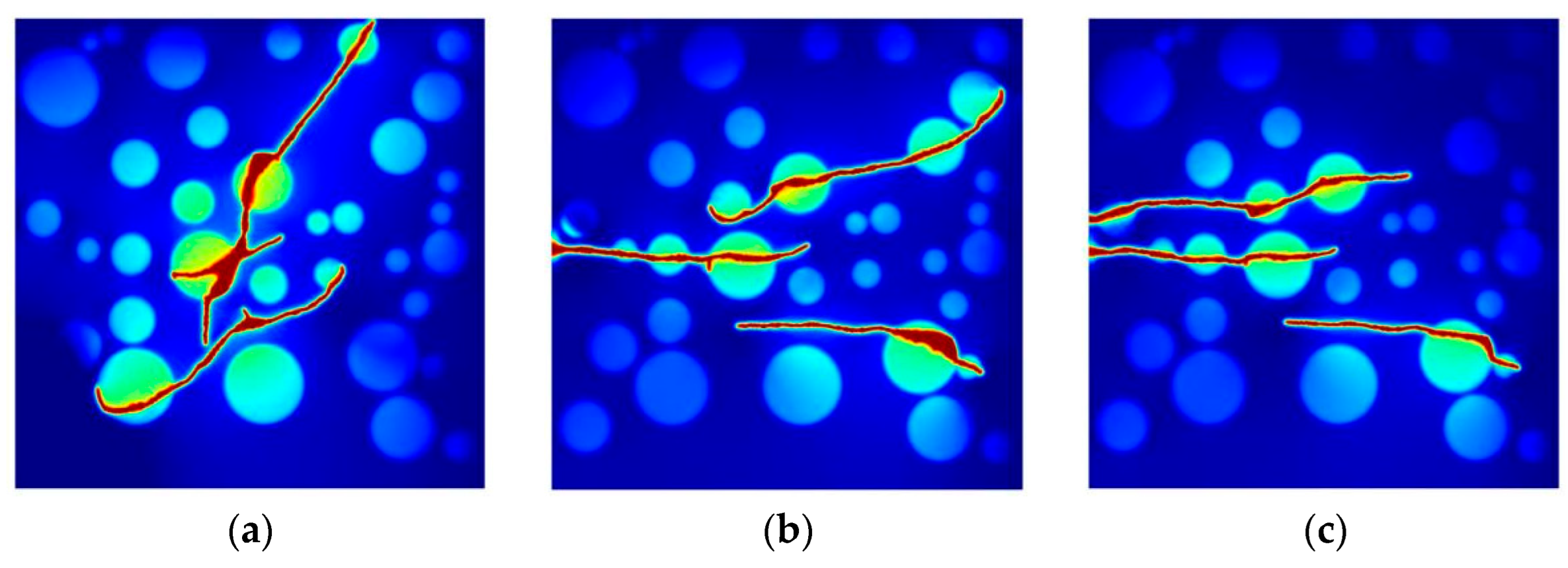
The propagation pattern reveals strong dependence on the particle component distribution and concentration (Figure 6). As shown in Figure 7, the final damage area for Class I reservoirs (80% brittle particles) measures approximately 1.5 × 10³ m², representing 25% and 50% increases over Class II (1.21 × 10³ m²) and Class III (1.02 × 10³ m²) reservoirs, respectively. This enhanced fracturing results from the relatively uniform and concentrated distribution of brittle minerals in Class I reservoirs, which creates continuous “weak channels” that facilitate smoother fracture propagation. These channels enable fractures to extend with minimal deflection while maintaining strong alignment with the maximum stress direction, establishing a positive feedback mechanism. The resulting path curvature index R (L_actual/L_straight) measures approximately 1.08. In contrast, Class II and III reservoirs exhibit higher curvature indices (1.32 and 1.53, respectively), reflecting the discrete distribution of brittle particles and associated energy barriers during fracture propagation.

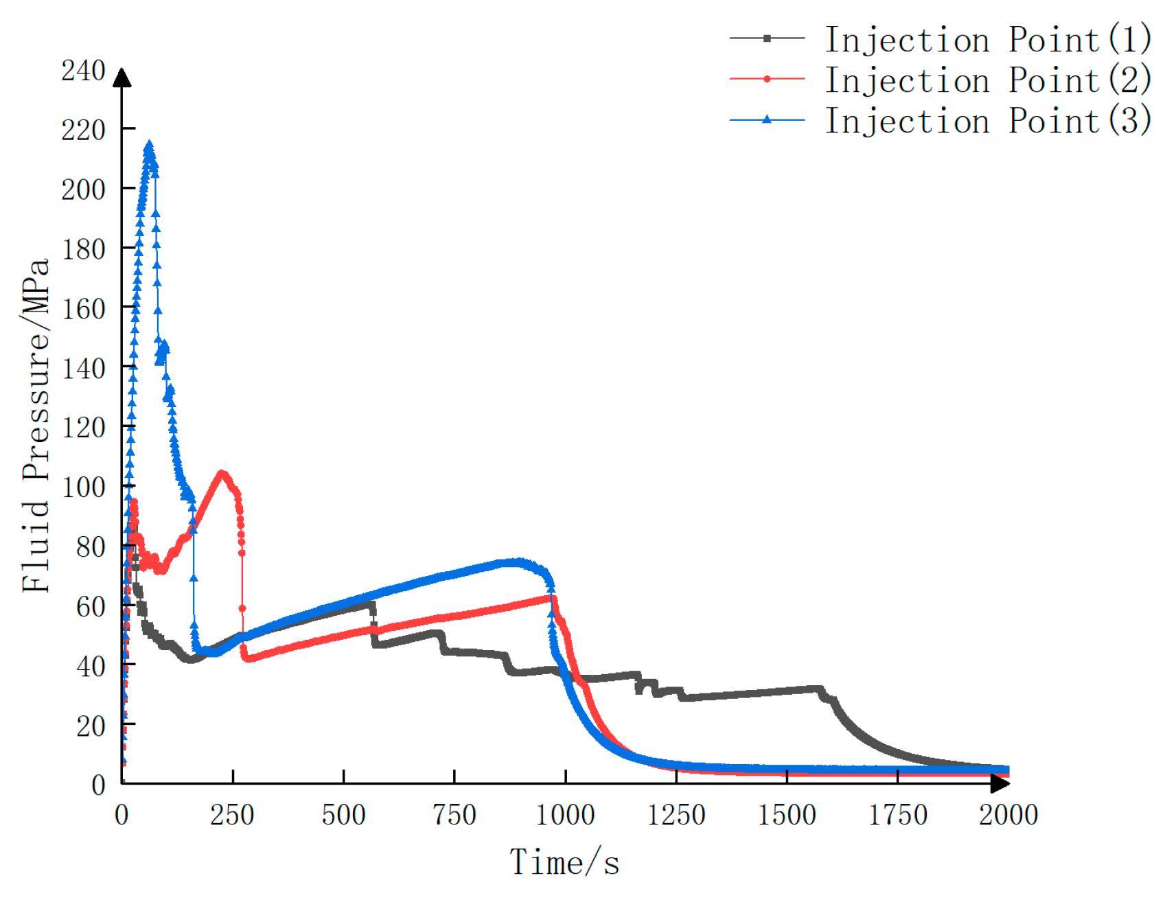
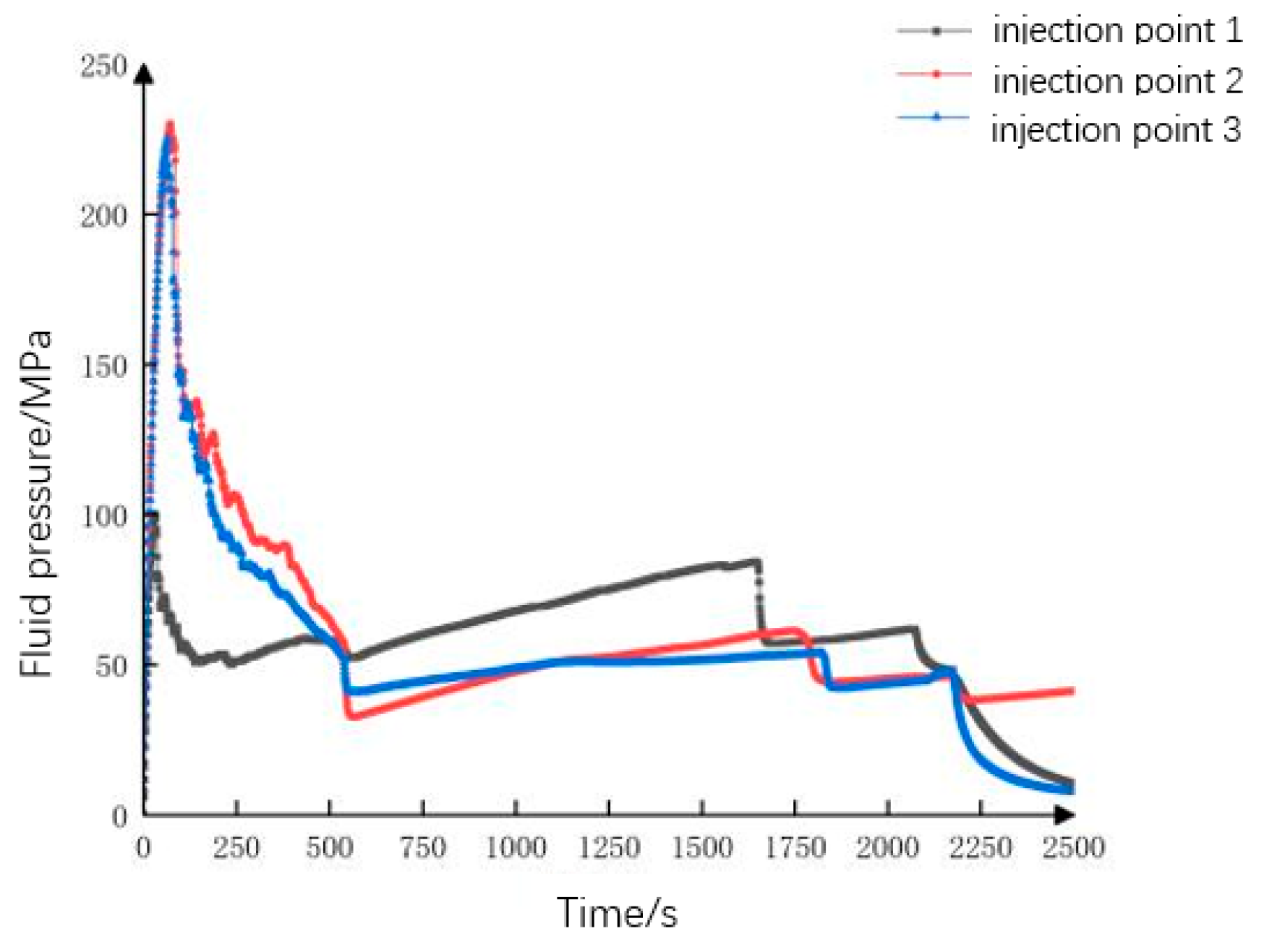
Figure 8 shows fracturing time (s) on the horizontal axis and fluid pressure (MPa) on the vertical axis. The three curves correspond to injection points at the model center and 15 m above and below it, respectively. Peak pressure corresponds to the moment of fracture initiation. Figure 7 shows fracturing time (s) on the horizontal axis and damage area (m²) on the vertical axis. Reservoir Types I, II, and III correspond to high, medium, and low proportions of brittle minerals, respectively, with the damage area reflecting the fracture propagation extent.

Figure 8 demonstrates that pressure variations at injection points effectively characterize crack initiation behavior. The peak initiation pressure at injection point 3 (matrix region) reaches 200 MPa, significantly exceeding values at points 1 and 2. This pressure differential indicates that brittle granular regions exhibit lower rupture thresholds compared to muddy matrices, requiring less energy for crack initiation. Consequently, cracks preferentially nucleate and propagate through brittle regions, exhibiting an overall “soft-preferential” propagation pattern.

Numerical analysis of pressure variation curves for the three reservoir types reveals distinct pressure fluctuation characteristics. Type I reservoirs exhibit a fluid pressure standard deviation of ${\sigma }_{\mathrm{p}}$ = 28 MPa, while Types II and III show progressively greater deviations of ${\sigma }_{\mathrm{p}}$ = 42 MPa and ${\sigma }_{\mathrm{p}}$ = 64 MPa, respectively. These substantial standard deviations indicate significant temporal pressure variations, demonstrating an inverse relationship between brittle particle content and pressure stability. Specifically, reservoirs with lower brittle particle ratios exhibit more pronounced energy fluctuations during fracture propagation, resulting in greater local stress field variability. This phenomenon is further exacerbated by particle–matrix interface effects, which amplify local energy and stress field disturbances.

3.2.2. Analysis of the Effect of Horizontal Stress Differences

Stress anisotropy is uniformly quantified using the horizontal stress difference coefficient $K_h$:$K_h$ ≥ 0.7, which denotes low anisotropy (small stress difference), while $K_h$ ≤ 0.3 indicates high anisotropy (large stress difference). The core principle concerns stress direction-constrained strength rather than mere stress magnitude, thereby avoiding conceptual confusion. The stress propagation limit denotes the range within which stress effectively drives crack growth, judged by the stress concentration factor $K_t$ ≤ 1.0: propagation follows the direction of maximum principal stress under high anisotropy, whereas it occurs uniformly under low anisotropy. This is not a fixed distance, thus eliminating cognitive bias.

The horizontal stress difference serves as the critical factor controlling formation fracture initiation pressure, propagation direction, and morphology. As defined in Equation (17) by the horizontal stress difference coefficient, we examine fracture initiation and propagation behaviors using the Class II reservoir’s particle mineral composition ratio and distribution as a representative case (Figure 9).

Table 6. Horizontal stress parameters for different types of reservoirs.

	$\mathbf{Maximum} \mathbf{Horizontal} \mathbf{Stress} {\mathit{S}}_{\mathit{h}}$	$\mathbf{Minimum} \mathbf{Horizontal} \mathbf{Stress} {\mathit{S}}_{\mathit{v}}$	$\mathbf{Stress} \mathbf{Difference} \mathit{\Delta }\mathit{\sigma }$	$\mathbf{Stress} \mathbf{Anisotropy} \mathbf{Coefficient} {\mathit{K}}_{\mathit{h}}$	Classification Criteria
Category I	30 MPa	28 MPa	2	0.92	≥0.7
Category II	30 MPa	23 MPa	7	0.69	0.3–0.7
Category III	30 MPa	17 MPa	13	0.24	≤0.3

presents the simulated horizontal stress parameters and classification criteria for different reservoir types.

$$K_h=1-{\displaystyle \frac{S_h-S_v}{S_v}}$$

(17)

$K_h$ denotes the horizontal stress difference coefficient; $S_h$ represents the maximum horizontal principal stress (MPa); $S_v$ denotes the minimum horizontal principal stress.

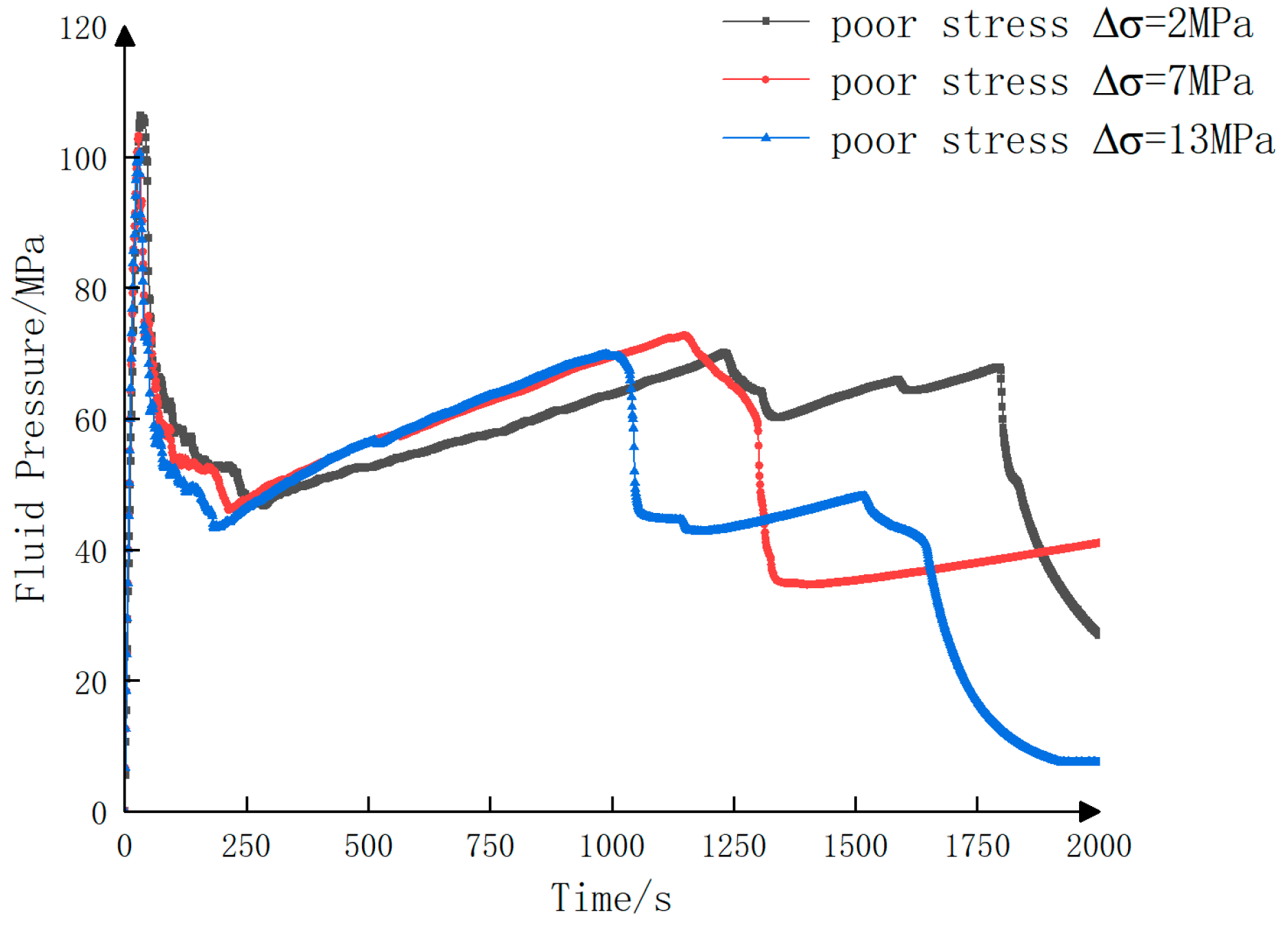
Numerical simulations of three reservoir types using the phase-field model demonstrate a significant negative correlation between fracture initiation pressure and stress difference (Figure 10). The initiation pressures measure approximately 106.8 MPa for Class I reservoirs, exceeding those of Class II (103.4 MPa) and Class III (99.3 MPa) reservoirs. This behavior stems from preferential crack initiation and propagation along directions favoring energy release and stress concentration relief. In Class I reservoirs, the relatively balanced initial stress state with smaller stress differences requires overcoming higher energy barriers for fracture initiation, consequently resulting in elevated initiation pressures.

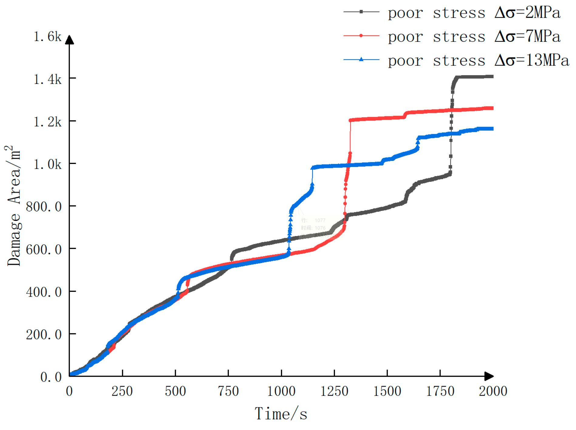
Fracture morphology evolution exhibits significant variations among reservoir types (Figure 11). Class I reservoirs develop damage areas of approximately 1.42 × 10³ m², representing 14% and 22% increases over Class II (1.25 × 10³ m²) and Class III (1.16 × 10³ m²) reservoirs, respectively. These results indicate greater potential for complex fracture network formation in Class I reservoirs, attributable to a dual control mechanism combining stress direction effects and mineral heterogeneity perturbations. Under high stress difference conditions (Class III reservoirs), the stress concentration coefficient K_t (local maximum stress to average stress ratio) reaches 3.2 in the maximum principal stress direction—significantly exceeding values for Class II (K_t = 2.4) and Class I (K_t = 1.3) reservoirs. This demonstrates enhanced lateral crack constraints and highly directional propagation, where stress direction effects dominate over particle distribution influences. Conversely, Class I reservoirs under low stress differences (Δσ ≤ 7 MPa) exhibit mechanical contrasts between brittle particles and muddy matrices that trigger local energy dissipation and redistribution. When the particle-induced stress perturbation (Δσ/σH ≤ 0.23) exceeds the macroscopic stress gradient, mineral heterogeneity becomes the predominant factor controlling fracture morphology.

3.2.3. Analysis of the Impact of Natural Cracks

Natural fractures exert a significant influence on expansion. This study, based on field core observations (fracture tortuosity of 1.1~1.3, roughness Ra = 20~50 μm, and calcite filling rate of 15%~30%), employs an equivalent coefficient correction model to approximate the characteristics of actual fractures.

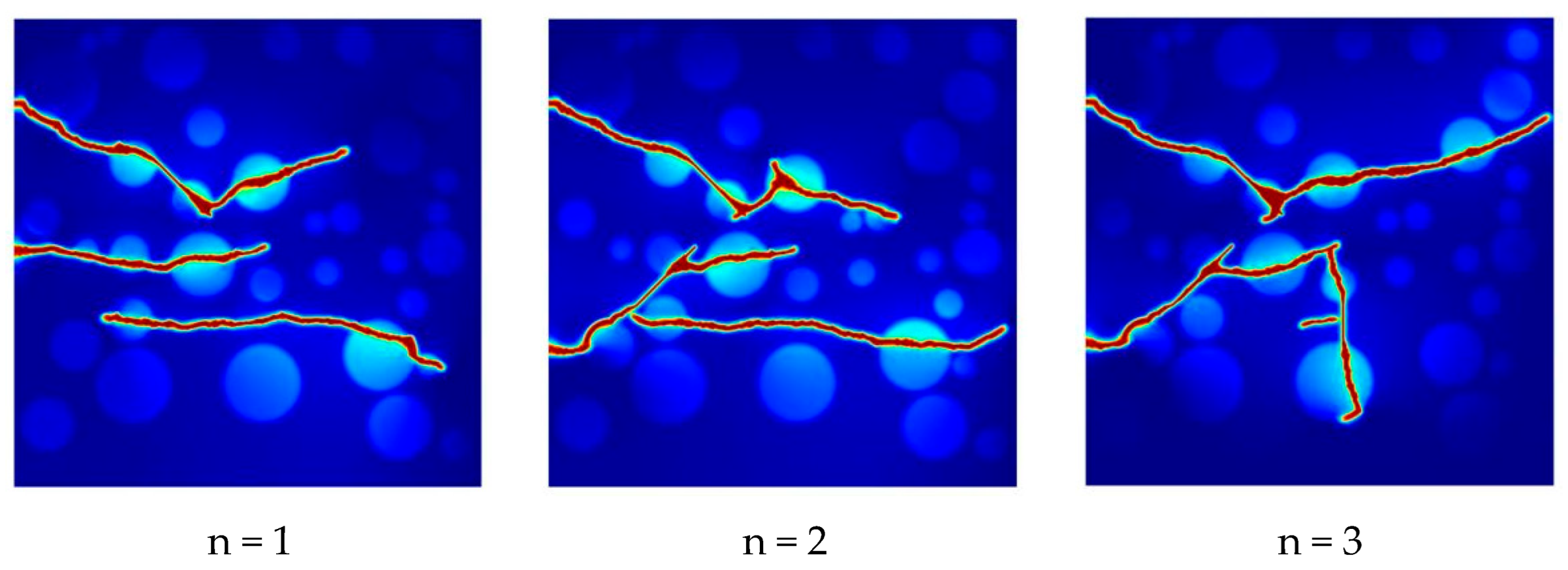
Natural fractures exert extensive and critical influences on fracture propagation. In the Heroes’ Ridge shale reservoirs, different natural fracture types distinctly affect fracture network complexity. Using the Class II reservoir’s particle mineral distribution and stress difference conditions as a representative case, we simulate reservoirs containing natural fractures with varying angles and quantities (n = 1, 2, and 3). The simulation results reveal the following characteristics.

Figure 12 demonstrates that fracture propagation paths and patterns are significantly influenced by natural fracture quantity and orientation. In reservoirs containing a single natural fracture, hydraulic fractures connect with the natural fracture under combined particle distribution and stress field effects, then propagate along the natural fracture tip direction due to stress concentration. Reservoirs with two natural fractures exhibit more complex propagation behavior, where fracture bifurcation and intersection during propagation create denser fracture networks. For triple-natural-fracture systems, propagation paths become jointly controlled by all three fractures, generating more complex network patterns. However, the overall fracture propagation range becomes more limited due to premature path alterations caused by natural fractures, resulting in mutual interference between hydraulic fractures.

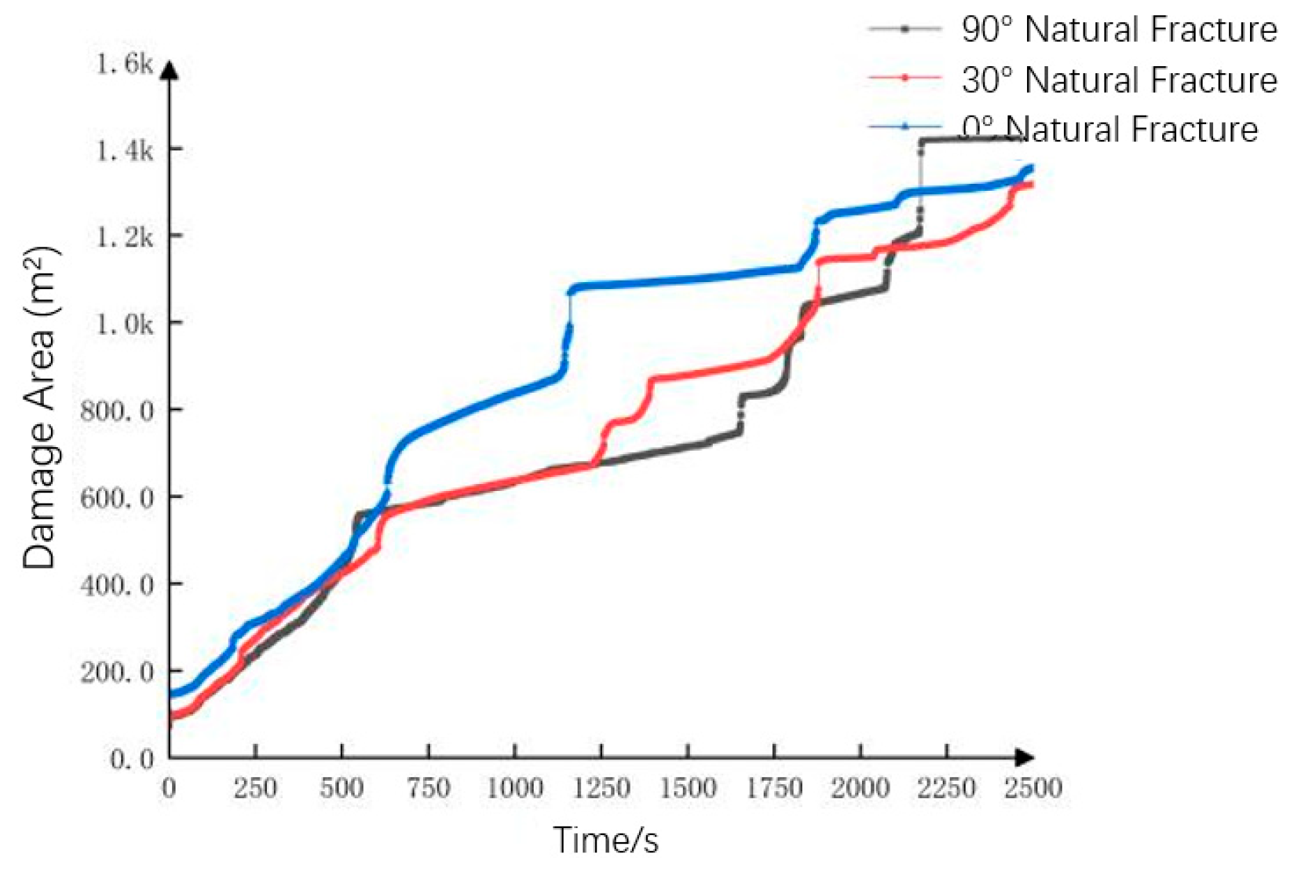
Figure 13 presents the fluid pressure evolution in a dual-natural-fracture reservoir. At injection point 2, fracture initiation through brittle particles occurs during t = 252–345 s. Following a pressure redistribution phase, natural fracture interconnection at t = 670 s triggers abrupt pressure decline. This cyclic pattern demonstrates how pressure dynamics respond to medium heterogeneity and natural fracture networks, where particle distribution governs the initial propagation direction while natural fractures alter stress fields and flow paths. Figure 14 compares the damage area evolution across reservoir types. The dual-natural-fracture reservoir achieves maximum damage (∼1130 m²), exceeding single-fracture (∼950 m²) and triple-fracture (∼880 m²) cases. The reduced damage in triple-fracture systems stems from premature main fracture bifurcation caused by new vertical fractures. These results underscore the critical importance of accurately predicting natural fracture distribution and orientation for reliable fracture propagation forecasting. The simulation results were validated using microseismic data from two boreholes, with a fracture propagation error margin of ≤7%, thereby demonstrating the model’s validity.

3.2.4. Fractability Evaluation Analysis

Fracture propagation is fundamentally governed by the combined effects of natural fracture distribution, brittle mineral particle arrangement, and in situ stress fields.

Table 7. Simulated conditions and geostress parameters for three types of reservoirs.

	$\mathbf{Brittleness} \mathbf{Index} \mathit{B}\mathit{I}$	$\mathbf{Stress} \mathbf{Anisotropy} \mathbf{Coefficient} {\mathit{K}}_{\mathit{h}}$	$\mathbf{Natural} \mathbf{Fracture} \mathbf{Density} {\mathit{\rho }}_{\mathit{a}}$	Composite Fractability Index FI
Type I	0.8	0.92	0.058	0.59
Type II	0.5	0.69	0.038	0.41
Type III	0.3	0.24	0.008	0.19

summarizes the simulation conditions and geomechanical parameters for three reservoir classifications:

Type I: High brittleness/low stress difference/high fracture density.

Type II: Medium brittleness/medium stress difference/medium fracture density.

Type III: Low brittleness/high stress difference/low fracture density.

The numerical simulation results for these reservoir types demonstrate the following key behaviors:

$$\mathrm{FI}={\displaystyle \frac{BI+K_h+{\rho }_a}{3}}$$

(18)

In the formula, BI denotes the standardized brittleness index ($B{I}_{std}$). The stress difference coefficient $K_h$ and fracture line density ${\rho }_a$ are standardized using the min-max method ($X_{std}={\displaystyle \frac{X-X_{min}}{X_{max}-X_{min}}}$), with all three indicators normalized to the [0, 1] range and each assigned a weight of 1/3 to ensure consistent computational logic. The physical significance of the standardized compressibility index FI becomes more explicit: Type I reservoir FI = 0.59 (all three indicators in the high-value range), Type II FI = 0.41 (moderate level), Type III FI = 0.19 (low-value range), corresponding precisely to the quantified results of fracture propagation effects.

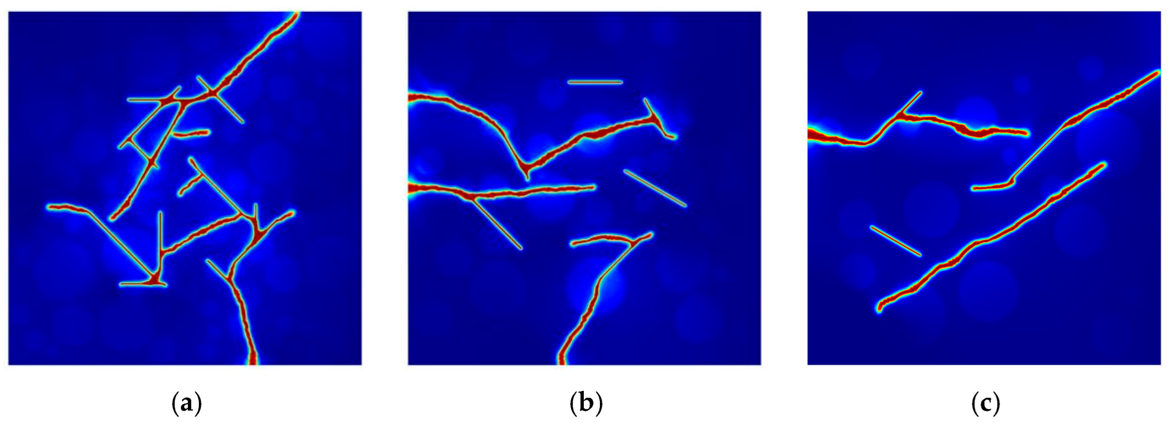
The fracture line density ${\rho }_a$ is defined as the ratio of the natural fracture area of the reservoir to the total area of the reservoir (Figure 15). It is used to classify the degree of natural fracture development in reservoirs: well-developed when ${\rho }_a$ ≥ 0.05, moderately developed when 0.01 ≤ ${\rho }_a$ < 0.05, and poorly developed when ${\rho }_a$ < 0.01. The fractability index (FI) is a comprehensive indicator that combines three equally weighted factors—the brittleness index, stress difference coefficient, and natural fracture influence—each assigned a weight of 1/3, as expressed in Equation.

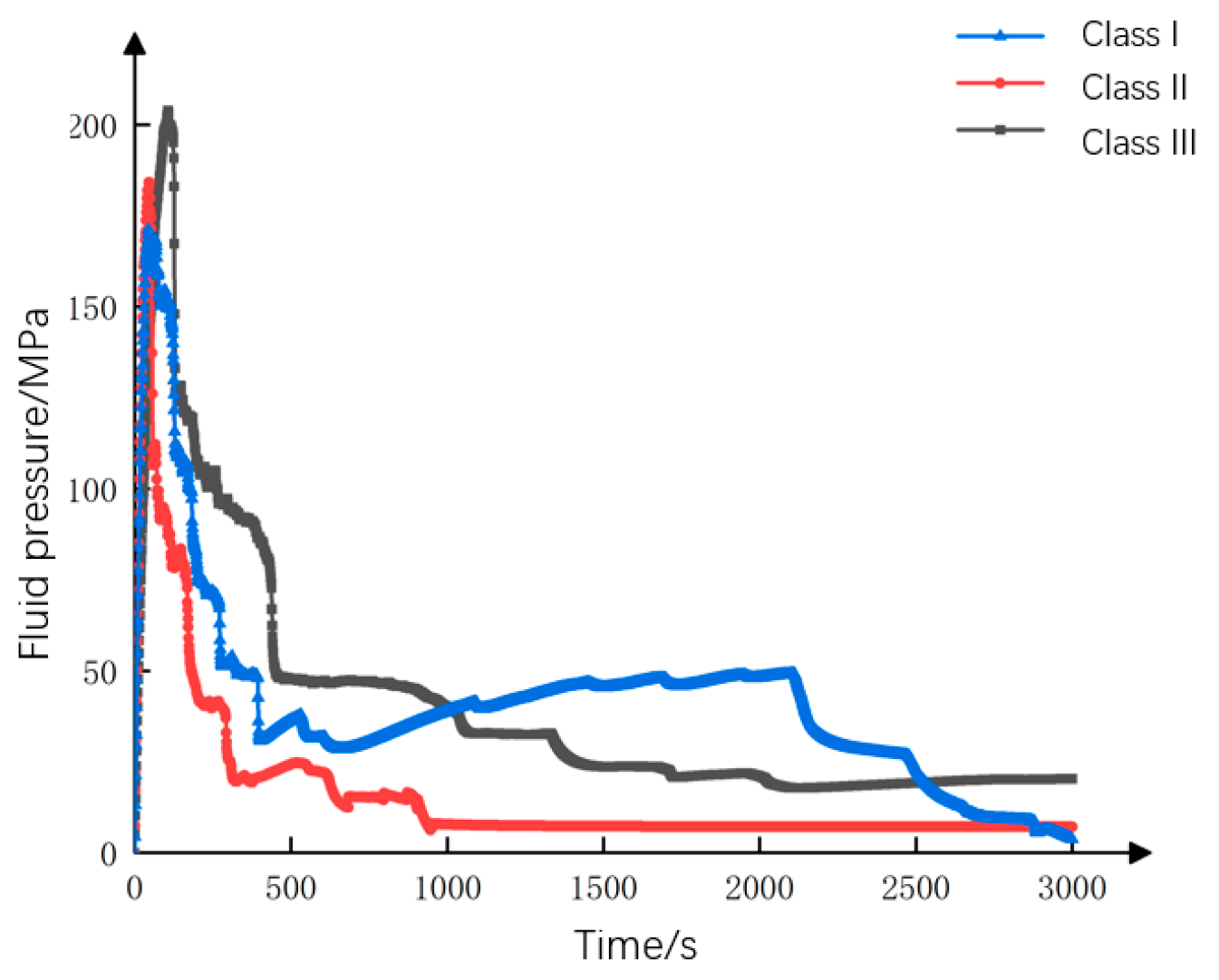
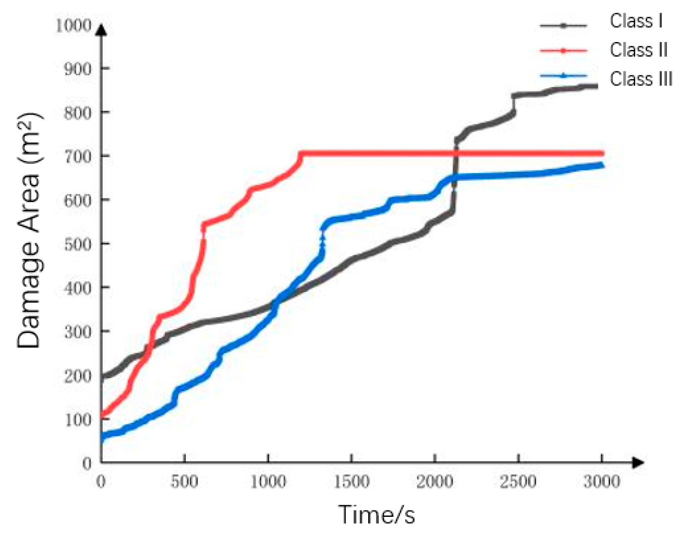
Numerical simulations reveal that the brittle mineral content significantly influences the fracture initiation energy. In Class I reservoirs (80% brittle particles), the critical initiation pressure measures 165 MPa, representing 8.3% and 21.4% reductions compared to Class II (180 MPa) and Class III (210 MPa) reservoirs, respectively (Figure 16). This demonstrates that brittle phases simultaneously reduce fracture toughness and govern rock mechanical properties, providing the material foundation for complex fracture network development. The stress difference coefficient quantifies in situ stress field heterogeneity, controlling fracture network complexity through propagation direction regulation. Class I reservoirs exhibit relatively unconstrained multi-directional propagation due to lower stress differences, whereas Class III reservoirs show strongly directional growth aligned with the maximum principal stress, reflecting enhanced stress anisotropy that inhibits fracture deflection. Natural fracture line density affects damage evolution through dual mechanisms: (1) providing fluid flow pathways that reduce fracturing fluid leak-off and (2) generating stress concentrations that promote secondary fracture initiation (Figure 17). Class I reservoirs develop 862 m² damage areas, exceeding Class II (715 m²) and Class III (694 m²) by 20.6% and 24.2%, respectively. Fracture pattern analysis shows Class I reservoirs form radial networks through natural fracture interactions, while Class III reservoirs typically produce simple, non-branching fractures.

Phase-field numerical simulations elucidate the multifactorial synergistic mechanism governing hydraulic fracture behavior, characterized by the following: (1) brittleness-dominated initiation, (2) stress-difference-guided propagation, and (3) natural-fracture-perturbed pathways. These results establish quantitative thresholds for complex fracture network formation: a brittleness index (BI) ≥ 0.6 ensures favorable initiation conditions, a stress anisotropy coefficient (K_h) ≥ 0.7 maintains propagation freedom, and a fracture density (${\rho }_a$) ≥ 0.05 provides sufficient flow pathways for effective stress perturbation. Through comprehensive parametric simulations, we developed the fractability evaluation index system, presented in

Table 8. Fractability evaluation classification criteria.

Evaluation Class	Classification Standard (FI)	Description
Class I	≥0.45	Capable of forming fully developed radial fracture networks
Class II	0.24–0.45	Capable of forming moderately complex fractures
Class III	≤0.24	Lacks conditions for fracture network

, which quantifies fracturing effectiveness across reservoir types. These findings provide novel theoretical insights for predicting fracture propagation patterns during actual hydraulic fracturing operations.

Two new weighted testing methods have been introduced, as presented in

Table 9. Testing method.

Reservoir Type	Equal Weighting	Expert Weighting	Entropy Rights Method
Class I	0.59	0.61	0.58
Class II	0.41	0.42	0.40
Class III	0.19	0.18	0.20

. Expert weighting method: Based on fracturing engineering experience, with a BI weighting of 0.4 (fracture initiation dominant), $K_h$ weighting of 0.3 (fracture propagation oriented), and ${\rho }_a$ weighting of 0.3 (path disturbance). Entropy-weighted method: Calculated from entropy values of 100 core data sets, with a BI weighting of 0.38, Kh weighting of 0.35, ${\rho }_a$ weighting of 0.27 (objectively reflecting indicator information content).

Quantifying uncertainty using the coefficient of variation (CV) for the weighted method:

• Class I reservoir CV = 2.8%, uncertainty range [0.57, 0.61];
• Class II reservoir CV = 2.4%, uncertainty range [0.40, 0.42];
• Class III reservoir CV = 5.3%, uncertainty range [0.18, 0.20].

All reservoir uncertainties remain < 6%, indicating that compressibility evaluation results are minimally affected by the weighting method, with classification conclusions (Class I > Class II > Class III) being stable and reliable.

To validate the composite brittleness index and threshold, field fracturing data from three additional target blocks with distinct well sections (well depths of 2800 m, 3000 m, and 3200 m) were incorporated: Section 1 (BI = 0.78; ${\rho }_a$ = 0.056) corresponds to FI = 0.58, with a fracturing treatment volume of 1280 m³, showing a deviation ≤ 5% from simulation results; Section 2 (BI = 0.52; ${\rho }_a$ = 0.035) corresponds to FI = 0.40, with a treatment volume of 920 m³, showing a deviation ≤ 7%; Section 3 (BI = 0.31; ${\rho }_{\mathrm{a}}$ = 0.009) corresponds to FI = 0.21, with a modified volume of 680 m³ and a deviation ≤ 6%. This validates the suitability of the index and threshold for the target block.

4. Conclusions

This study establishes a hydromechanically coupled phase-field fracture model and develops a comprehensive fractability evaluation system to analyze hydraulic fracture propagation in the Heroes’ Ridge shale reservoir. The key findings are as follows:

(1)

Brittle Mineral Dominance—Fracture propagation is primarily controlled by the brittle particle distribution, exhibiting “soft-preferential” propagation patterns (path curvature index: Class I = 1.08 vs. Class III = 1.53). Reservoirs with >80% brittle minerals (Class I) demonstrate 20.6% larger damage areas (862 m²) and 8.3% lower initiation pressures (165 MPa) than Class III reservoirs, confirming that brittle phases reduce fracture toughness while enhancing network complexity.

(2)

Stress Difference Control—A strong negative correlation exists between the horizontal stress difference ($K_h$) and initiation pressure (R² = 0.92). Mineral heterogeneity governs fracture morphology at Δσ ≤ 7 MPa (σ_h/σH ≤ 0.23), while stress orientation dominates when $K_h$≥ 0.7, limiting propagation to ±15° of the σ₁ direction.

(3)

Natural Fracture Effects—Natural fractures (${\rho }_a$ ≥ 0.05) enhance complexity by reducing fluid leak-off (18–25%) and promoting secondary fractures (30–40% density increase) via stress perturbations.

(4)

Through comprehensive analysis of the influence of various factors on fracture propagation, an integrated compressibility evaluation index has been established. This systematically elucidates the synergistic mechanism involving multiple factors: ‘brittle-dominated initiation, stress gradient-guided propagation, and natural fracture disturbance pathways’. This index and its threshold (FI ≥ 0.45 for Class I reservoirs) have been validated by field data from three wells in the target block (deviation ≤ 7%). It also accounts for reservoir heterogeneity: for high-porosity reservoirs (φ ≥ 10%), the FI threshold is recommended to be lowered to 0.40; for deep high-pressure reservoirs ($p$ ≥ 200 MPa), the index should be applied after modifying fracture energy using Equation (3a) to enhance its universality.

(5)

Drawing upon recent methodological advances such as porous elastic phase coupling and adaptive solving, the hydraulic–mechanical coupling logic and solution strategy have been optimized. The proposed heterogeneous reservoir simulation approach balances accuracy and efficiency, providing an engineering-practical method for complex shale reservoir fracturing simulations.

The core innovation of this study lies in developing a coupled analysis method for “hydraulic–mechanical phase damage” tailored to specific reservoirs by optimizing the coupling mechanism of existing phase-field models, thereby deriving quantitative thresholds for the comprehensive brittleness index. Although the study does not introduce an entirely novel theoretical framework, it achieves the precise implementation of existing models in specific reservoir fracturing evaluations through a “model parameter calibration + field data validation” pathway. This addresses the limitations of traditional methods, which primarily rely on qualitative descriptions and lack practical applicability. The proposed threshold has been validated through fracturing operations in two field wells, demonstrating significantly enhanced treatment effectiveness and confirming the practical value of the research. These findings provide a more robust theoretical basis for optimizing efficient fracturing parameters and modifying production plans in shale reservoirs, thereby advancing the effective development of unconventional oil and gas resources.

References

1. Zhao, C.; Liu, J.; Liu, J. Unconventional Natural Gas Systems and Their Exploration Prospects in China. J. Oil Gas Technol. 2009, 31, 193–195. [Google Scholar]
2. Zhou, Z.; Cheng, W.; Wei, Z.; Jiang, G. Numerical simulation of hydraulic fracture initiation and propagation based on BEM. Prog. Geophys. 2020, 35, 807–814. [Google Scholar]
3. Saber, E.; Qu, Q.; Sarmadivaleh, M.; Aminossadati, S.M.; Chen, Z. Propagation of multiple hydraulic fractures in a transversely isotropic shale formation. Int. J. Rock Mech. Min. Sci. 2023, 170, 105510. [Google Scholar] [CrossRef] [Scilit]
4. Zhao, B.; Hu, M.; Wu, T. A hybrid displacement discontinuity element method for hydraulic fracture propagation. Pet. Geol. Oilfield Dev. Daqing 2020, 39, 104–111. [Google Scholar]
5. Fang, X.-j.; Jin, F. Extended Finite Element Method Based on Abaqus. Eng. Mech. 2007, 24, 6–10. [Google Scholar]
6. Yi, L.; Hu, B.; Li, X. Calculation model of hydraulic crack vertical propagation in coal-sand interbedded formation based on the phase field method. J. China Coal Soc. 2020, 45, 706–716. [Google Scholar]
7. Wang, X.; Lu, D.; Li, P. A novel hybrid model for hydraulic fracture simulation based on peridynamic theory and extended finite element method. Theor. Appl. Fract. Mech. 2023, 123, 103731. [Google Scholar] [CrossRef] [Scilit]
8. Wu, J.; Li, J. Continuum Damage Mechanics Model and Smeared-crack Model for Concrete. J. Tongji Univ. Nat. Sci. 2004, 11, 1428–1432. [Google Scholar]
9. Zhou, S.; Zhuang, X.; Rabczuk, T. Phase-field modeling of fluid-driven dynamic cracking in porous media. Comput. Methods Appl. Mech. Eng. 2019, 350, 169–198. [Google Scholar] [CrossRef] [Scilit]
10. Francfort, G.A.; Marigo, J.-J. Revisiting brittle fracture as an energy minimization problem. J. Mech. Phys. Solids 1998, 46, 1319–1342. [Google Scholar] [CrossRef] [Scilit]
11. Bourdin, B.; Francfort, G.A.; Marigo, J.J. Numerical experiments in revisited brittle fracture. J. Mech. Phys. Solids 2000, 48, 797–826. [Google Scholar] [CrossRef] [Scilit]
12. Miehe, C.; Welschinger, F.; Hofacker, M. Thermodynamically consistent phase-field models of fracture: Variational principles and multi-field FE implementations. Int. J. Numer. Methods Eng. 2010, 83, 1273–1311. [Google Scholar] [CrossRef] [Scilit]
13. Wheeler, M.F.; Wick, T.; Wollner, W. An augmented-Lagrangian method for the phase-field approach for pressurized fractures. Comput. Methods Appl. Mech. Eng. 2014, 271, 69–85. [Google Scholar] [CrossRef] [Scilit]
14. Liu, G.; Li, Q.; Zuo, Z. Implementation of a staggered algorithm for a phase field model in ABAQUS. Chin. J. Rock Mech. Eng. 2016, 35, 1019–1030. [Google Scholar]
15. Liu, J.; Xue, Y.; Gao, F.; Teng, T.; Liang, X. Propagation of hydraulic fractures in bedded shale based on phase-field method. Chin. J. Geotech. Eng. 2022, 44, 464–473. [Google Scholar]
16. Li, M.; Li, S.; Zuo, J.; Wang, Z.; Lei, P.; Xue, X. Numerical Simulation of Three-point Bending Failure Behavior of Basalt Based on Phase Field Method. Sci. Technol. Eng. 2022, 22, 13441–13449. [Google Scholar]
17. Zhao, X.; Wang, G.; Li, Y.; Sun, Q.; Lai, J.; Shen, Y.; Wu, K.; Li, D.; Wang, S.; Han, Z. Development characteristics and logging identification of natural fractures in shale oil reservoirs of the Yingxiongling area, Qaidam Basin. Nat. Gas Geosci. 2025, 36, 713–733. [Google Scholar]
18. Wan, Y.; Wang, X.; Lei, F.; Zhang, D.; Wen, Y.; Zhong, Y. Compressibility evaluation and application E32 shale oil in Yingxiongling Area, Qaidam Basin. Unconv. Oil Gas 2024, 11, 120–129. [Google Scholar]
19. Zhou, S.; Zhuang, X.; Rabczuk, T. A phase-field modeling approach of fracture propagation in poroelastic media. Eng. Geol. 2018, 240, 189–203. [Google Scholar] [CrossRef] [Scilit]
20. Xie, G.; Lin, H.; Liu, S.; Liu, Y.; Wan, Y.; Zhang, C.; Li, Y.; Cui, R.; Lei, F.; Sui, G.; et al. Innovation and practice of geology and engineering integrated fracturing technology for shale oil in Yingxiongling area in the western Qaidam Basin. China Pet. Explor. 2023, 28, 105–116. [Google Scholar]
21. Miehe, C.; Hofacker, M.; Welschinger, F. A phase field model for rate-independent crack propagation: Robust algorithmic implementation based on operator splits. Comput. Methods Appl. Mech. Eng. 2010, 199, 2765–2778. [Google Scholar] [CrossRef] [Scilit]
22. Lee, S.; Wheeler, M.F.; Wick, T. Pressure and fluid-driven fracture propagation in porous media using an adaptive finite element phase field model. Comput. Methods Appl. Mech. Eng. 2016, 305, 111–132. [Google Scholar] [CrossRef] [Scilit]
23. Zhou, S.; Zhuang, X.; Zhu, H.; Rabczuk, T. Phase field modelling of crack propagation, branching and coalescence in rocks. Theor. Appl. Fract. Mech. 2018, 96, 174–192. [Google Scholar] [CrossRef] [Scilit]
24. Sneddon, I.N.; Lowengrub, M. Crack Problems in the Classical Theory of Elasticity; John Wiley & Sons: Hoboken, NJ, USA, 1969. [Google Scholar]
Figure 1. Characterization of diffusion by phase-field method for sharp cracks: (a) sharp crack; (b) diffuse fracture. The arrows in the figures represent the direction of applied boundary loads on the model boundaries, as well as the gradient direction of the phase field variable during crack propagation. The color gradient (from blue to red) indi-cates the distribution of the phase field variable, where red regions denote the crack tip and high-energy areas.
Energies 19 00922 g001
Figure 2. Geometry and boundary conditions of the medium at internal fluid pressure.
Energies 19 00922 g002
Figure 3. Crack morphology and fluid pressure changes. The color coding in these figures represents the magnitude of the key physical field variable (e.g., fluid pressure or stress) in our COMSOL simulation. Dark blue indicates the minimum value of the variable, while the gradient through cyan, green, and yellow to red shows an increase in magnitude, with red representing the maximum value.
Energies 19 00922 g003aEnergies 19 00922 g003b
Figure 4. Comparison curve of displacement in Y-direction.
Energies 19 00922 g004
Figure 5. Non-homogeneous field geometry and boundary conditions. (a) Category I; (b) Category II; (c) Category III. The circles of different sizes in the figure represent the equivalent geometric size of natural fractures, where larger circles indicate fractures with larger aperture/extension length, medium circles represent fractures with moderate aperture/extension length, and smaller circles denote micro-fractures with smaller aperture/extension length.
Energies 19 00922 g005
Figure 6. Fracture morphologies of different types of reservoirs. (a) Category I; (b) Category II; (c) Category III. This figure is a cloud map of fluid migration/pressure field distribution from COMSOL simulation, with colors rep-resenting the magnitude of the physical field. Dark blue indicates the lowest value, light blue to cyan indicates moderate values, and yellow to orange-yellow indicates the highest values (e.g., fluid enrichment zones or high-permeability channels).
Energies 19 00922 g006
Figure 7. Comparison of damage areas in different types of reservoirs.
Energies 19 00922 g007
Figure 8. Variation in fluid pressure at different injection points in Class II reservoir.
Energies 19 00922 g008
Figure 9. Fracture morphologies of different types of reservoirs at the same moment of time. (a) Category I; (b) Category II; (c) Category III. This figure is a cloud map of fluid migration/pressure field distribution from COMSOL simulation, with colors rep-resenting the magnitude of the physical field. Dark blue indicates the lowest value, light blue to cyan indicates moderate values, and yellow to orange-red indicates the highest values (e.g., fluid enrichment zones or high-permeability channels).
Energies 19 00922 g009
Figure 10. Fluid pressure variation at injection point 1 for different reservoirs.
Energies 19 00922 g010
Figure 11. Comparison of damage areas in different types of reservoirs.
Energies 19 00922 g011
Figure 12. Fracture patterns in reservoirs with different numbers of natural fractures. This figure is a cloud map of fluid migration/pressure field distribution from COMSOL simulation, with colors representing the magnitude of the physical field. Dark blue indicates the lowest value, light blue to cyan indicates moderate values, and yellow to orange-red indicates the highest values (e.g., fluid enrichment zones or high-permeability channels).
Energies 19 00922 g012
Figure 13. Variation in fluid pressure at different injection points in natural fractured reservoir.
Energies 19 00922 g013
Figure 14. Comparison of damage areas in natural fractured reservoir at different angles.
Energies 19 00922 g014
Figure 15. Fracture patterns in different types of reservoirs. (a) Category I; (b) Category II; (c) Category III. This figure is a cloud map of fluid migration/pressure field distribution obtained from COMSOL simulation, with colors representing the magnitude of the physical field. Dark blue indicates the lowest value (e.g., background matrix with no fluid involvement), light blue to cyan indicates moderate values, and yellow to orange-red indicates the highest values (e.g., fluid-rich high-permeability fracture channels). The gray lines represent the initial natural fractures.
Energies 19 00922 g015
Figure 16. Variation in fluid pressure in different types of reservoirs.
Energies 19 00922 g016
Figure 17. Comparison of damage areas in different types of reservoirs.
Energies 19 00922 g017