GIS Partial Discharge Fault Diagnosis Based on Multi-Source Feature Fusion and ResNet-MLP

Abstract

Partial discharge (PD) signals in gas-insulated switchgear (GIS) exhibit complex characteristics, and single-modal feature recognition methods face limitations in achieving satisfactory diagnostic accuracy due to incomplete fault information representation. This paper proposes a multi-modal fault diagnosis framework that effectively integrates complementary information from different sensing modalities to improve defect identification performance. First, PRPD time-domain statistical features from HFCT measurements and frequency-domain features from UHF signals are extracted to construct a comprehensive hybrid feature set. Z-score normalization is applied to eliminate scale differences between heterogeneous features. Principal component analysis (PCA) is then employed for dimensionality reduction, preserving essential discriminative information while removing redundancy. Finally, a ResNet-MLP classifier with skip connections is designed to enhance nonlinear feature extraction and alleviate gradient vanishing problems in deep network training. Experimental validation on four typical defect types—protrusion defect, floating discharge, metal particle discharge, and surface discharge on insulator—demonstrates that the proposed method achieves 99.38% classification accuracy on the test set, with consistently high precision, recall, and F1-score across all categories. The proposed approach significantly outperforms standard MLP without residual connections, achieving 98.94% ± 0.49% accuracy compared to 95.47% ± 3.72% over 20 independent runs, demonstrating superior diagnostic accuracy and generalization capability for GIS insulation fault diagnosis.

1. Introduction

In China, both alternating current (AC) and direct current (DC) power transmission have advanced rapidly [1]. Against this backdrop, to meet the reliability and low-maintenance requirements of modern power systems, gas-insulated switchgear (GIS) offers a viable solution [2,3]. However, various insulation defects may occur inside GIS during manufacturing, transportation, installation, or long-term operation, which are important factors affecting its reliability. Partial discharge (PD), as an early indicator of insulation degradation, makes effective monitoring and diagnosis particularly crucial [4]. Early identification and accurate diagnosis of PD can not only prevent potential serious failures but also extend the service life of the equipment and reduce maintenance and replacement costs [5,6,7].

PD detection and diagnosis play a crucial role in ensuring the safe and reliable operation of GIS equipment. Among the various PD detection techniques, the phase-resolved partial discharge (PRPD) method based on high-frequency current transformer (HFCT) sensors is widely adopted in industrial applications [8]. In addition, ultra-high frequency (UHF) electromagnetic wave detection has also been extensively applied [9,10,11]. The PRPD technique captures pulse current signals and analyzes the relationship between discharge amplitude and phase angle, providing valuable statistical information for defect identification [12,13]. Each modality captures distinct physical characteristics of the discharge process, and their combination has the potential to provide a more comprehensive representation of the defect status.

Despite significant advances in PD signal acquisition and processing, accurate fault diagnosis remains challenging due to the complexity and variability of PD signals. Traditional diagnostic methods often rely on single-modality features, which may not fully capture the multifaceted characteristics of different defect types [14]. Moreover, conventional machine learning approaches, such as backpropagation (BP) neural networks and support vector machines (SVMs), face limitations in extracting nonlinear features from high-dimensional data, particularly when dealing with overlapping feature distributions among different fault categories [15,16]. The curse of dimensionality and the risk of overfitting further complicate the diagnosis task when dealing with limited sample sizes.

Some researchers have explored various approaches from both signal processing and pattern recognition perspectives. From the signal processing standpoint. Reference [17] proposed a combined singular value decomposition and variational mode decomposition (SVD-VMD) method for denoising PD signals, enhancing signal quality for subsequent analysis. From the pattern recognition standpoint, Reference [18] introduced a CNN-based deep learning method for PD pattern recognition in high-voltage cables, demonstrating superior feature extraction capabilities compared to traditional methods. To further improve diagnostic accuracy, Reference [19] developed a dual-channel feature fusion convolutional neural network (IFCNN) that integrates one-dimensional time-domain features with two-dimensional wavelet time-frequency map features for GIS defect classification. Reference [20] proposed an improved whale optimization algorithm (IWOA) for adaptively optimizing VMD and SVM parameters, combined with multi-scale permutation entropy (MPE) feature extraction to achieve GIS PD fault diagnosis. In [21], it developed an optimized CNN-based PD detection method for power cables, utilizing principal component analysis (PCA) for dimensionality reduction and a hybrid optimization algorithm to enhance recognition accuracy.

Motivated by these issues, this paper develops a lightweight multi-source feature fusion framework that couples interpretable statistical descriptors with a residual multilayer perceptron (ResNet-MLP) classifier. The proposed pipeline (1) extracts PRPD time-domain statistical features from HFCT measurements and frequency-domain features from UHF measurements to form a hybrid feature set; (2) applies Z-score normalization and principal component analysis (PCA) to obtain a compact representation [22]; and (3) employs a ResNet-MLP with skip connections to enhance nonlinear discrimination while maintaining good trainability under limited samples. This design aims to leverage multi-modal complementarity and improve diagnostic accuracy and generalization for typical GIS insulation defects. The proposed method is primarily designed for medium-voltage GIS and compact GIS installations, as well as high-voltage GIS compartments near cable terminations or bushings where both HFCT and UHF sensors can be effectively deployed.

The remainder of this paper is organized as follows. Section 2 describes the experimental platform for defect simulation and the PD measurement setup, along with the PRPD analysis of four typical defect types. Section 3 presents the feature extraction methods for both pulse current signals and UHF signals. Section 4 introduces the multi-feature fusion and dimensionality reduction process based on PCA. Section 5 details the ResNet-MLP network architecture and the training procedure, followed by a comparison of classification results. Finally, Section 6 concludes this paper with a summary of the main findings.

2. Simulated Defect Experimental Platform and Measurement Results

2.1. Defect Simulation and Data Processing

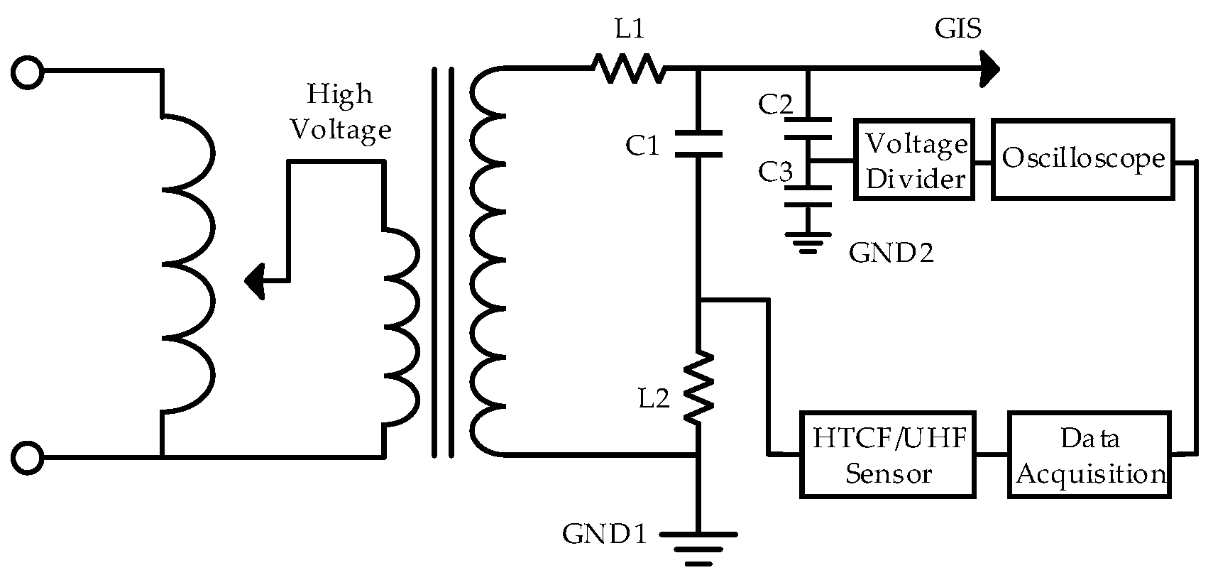
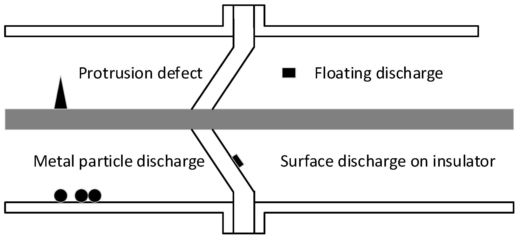
To comprehensively analyze the PD status of GIS equipment and assess its severity, this work simulates various defects occurring in GIS and designs four fault models: protrusion defect, floating discharge, metal particle discharge, and surface discharge on insulator. The structural diagram of the PD measurement device is shown in Figure 1. In Figure 1, the arrows indicate the connections to the GIS chamber. The four fault models used in this study are illustrated in Figure 2. This system mainly consists of a HFCT sensor and UHF sensor, an oscilloscope, and a data acquisition unit.

In the experiments to acquire pulsed current signals, the HFCT sensor was first installed at a designated location in the tested GIS system to couple and capture the high-frequency pulse current signals generated by PD. Then, the pulse generator was activated to inject a pre-set pulse current signal into the tested system to simulate or excite discharge conditions and verify signal transmission characteristics. The HFCT sensor performed real-time detection and recording of the injected signal. When the signal propagated to the PD defect location, it produced reflection and distortion characteristics related to the defect, resulting in a clear PD response in the acquired waveform. Simultaneously, the acquired signal was aligned with the power supply phase information using a synchronization system, providing a basis for subsequent phase-resolved analysis.

In the signal processing stage, the acquired pulse current signal was first input into the data acquisition unit for pre-processing and noise suppression, filtering out interference components and extracting effective discharge pulses. Then, the oscilloscope, using the power frequency cycle as the time base, divided the data within one cycle into several phase angle intervals and statistically counted the number of discharge pulses and their amplitude distribution within each phase interval. Finally, a PRPD pattern was generated based on the phase-amplitude-count statistical results, providing a basis for discharge mode recognition and characteristic comparison analysis of different defect types.

To capture UHF signals, the UHF sensor is externally mounted at the insulator window on the GIS enclosure, with its position adjusted to ensure optimal electromagnetic coupling. Unlike HFCTs, which capture conducted current pulses, the UHF sensor detects electromagnetic waves radiated by the rapid charge movement during PD events. These signals typically range from 300 MHz to 3 GHz and contain rich spectral information that can be used to characterize various insulation defects.

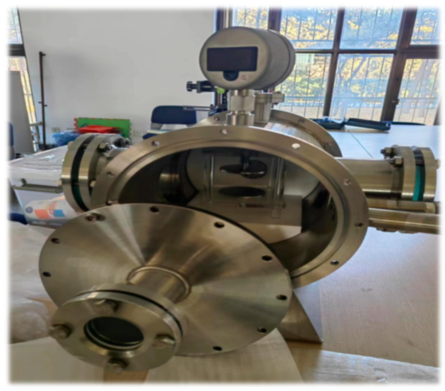
In the experimental setup, the HFCT sensor is installed at the grounding wire of the cable termination to capture conducted PD current pulses, which is consistent with typical field installation practices. The UHF sensor is externally mounted at the insulating spacer window on the GIS enclosure, requiring no internal access to the equipment. These sensor configurations are applicable to medium-voltage GIS and high-voltage GIS compartments near terminations where both sensors can achieve effective coverage, as shown in Figure 3.

2.2. PRPD Analysis of Four Defects

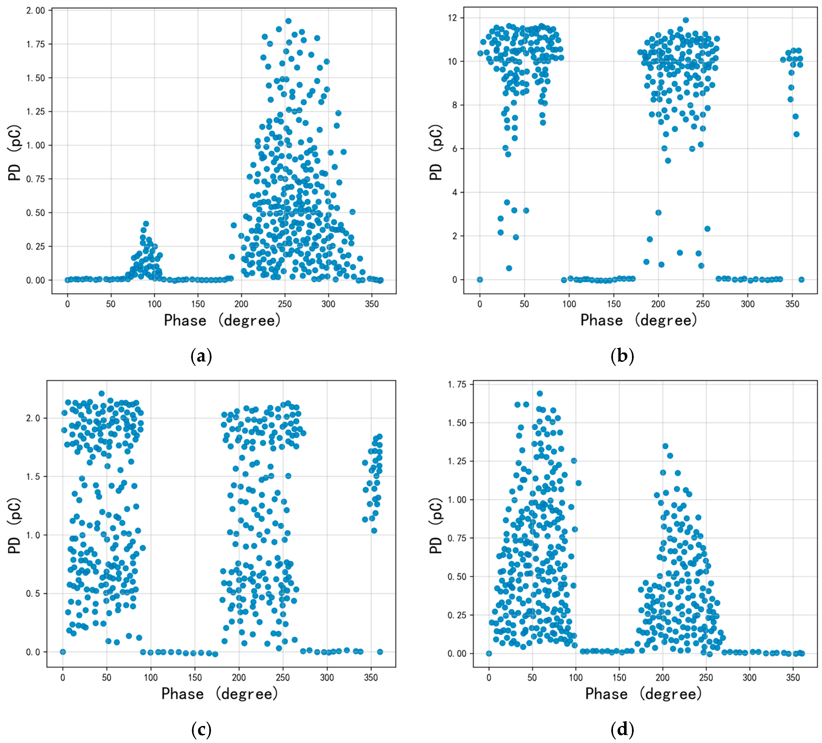
Through multiple trials, exploration, and comparison, the PD inception voltage of the model was determined to be 35 kV. To obtain stable, continuous, and repeatable PD signals, the subsequent experiments used a voltage set to 1.2 times the inception voltage, approximately 42 kV. Choosing 1.2 times the initiation voltage ensures stable and repeatable discharge activity while avoiding over-discharge that could damage the defect model. This voltage level is commonly used as a standard test condition in partial discharge experimental studies. The operating conditions were kept consistent at this voltage level to minimize the influence of voltage fluctuations on the discharge characteristics. For data acquisition, repeated tests and recordings were conducted for four typical fault models. 200 sets of PD data were collected for each model, resulting in a sufficient sample size to support subsequent feature analysis and comparative studies. The PRPD patterns corresponding to the four types of PD faults are summarized in Figure 4, which can be used to visually demonstrate the differences in phase distribution, discharge amplitude, and repetition rate among different fault types.

As shown in Figure 4, the PRPD patterns of different defect types exhibit significant differences in discharge phase distribution, amplitude level, and repetition rate, thus serving as an important basis for defect identification and mechanism analysis. Protrusion discharge is mainly concentrated in the middle and later stages of the phase angle, with generally low amplitude, and the pattern shows a relatively narrow-band, low-energy pulse distribution. This type of discharge is usually caused by local electric field distortion due to sharp points or burrs on the conductor surface. Floating discharge, on the other hand, exhibits relatively high amplitude and shows a clear clustering characteristic within a specific phase range. The PRPD pattern shows a higher frequency and greater dispersion of high-amplitude pulses. Its cause is usually related to the conductor or metal components being in an unreliable grounding or unstable potential state, such as floating metal pieces, loose connections, or potential drift caused by local insulation degradation. Metal particle discharge is usually distributed in two phase intervals in the pattern, with generally low amplitude, and the discharge points form corresponding phase clusters in the positive and negative half-cycles. This type of discharge is closely related to the spatial position of the particles in the electric field, their force state, and their contact or gap with the electrode/insulation surface. Surface discharge on insulators is also mainly concentrated in two phase intervals, with generally low amplitude, but its phase clustering morphology differs from that of metal particle discharge, often showing a more continuous or denser discharge band in the phase range where the electric field is more easily concentrated on the insulator surface. Its mechanism is usually related to increased surface conductivity caused by surface contamination, moisture, aging damage, or attached particles on the insulator surface.

In summary, protrusion defect is characterized by concentration in the middle and later stages, low amplitude; floating discharge is characterized by high amplitude, specific phase clustering; metal particle discharge is characterized by dual-phase clusters in positive and negative half-cycles, low amplitude; and surface discharge on insulator is characterized by dual-phase interval concentration due to surface effects and features related to the surface state.

3. Feature Extraction via Pulse Current Signal and UHF Data

3.1. Feature Extraction via Pulse Current Signal

3.1.1. The Formula for Feature Extraction

Clearly, by leveraging the aforementioned characteristics and differences, feature extraction from PRPD data provides a solid foundation for subsequent statistical analysis and defect type identification. The PRPD data collected each time are uniformly formatted and organized into a sample–feature matrix. The extracted time-domain features can then be grouped into three categories according to their physical meanings: amplitude statistics, higher-order statistics, and ratio-based features.

Amplitude statistics include peak value (P_max), mean value (μ), and root-mean-square value (R_MS). The peak value reflects the maximum amplitude of the signal, directly characterizing the transient intensity of PD and the occurrence of extreme discharge events, as shown in Equation (1). In cases of more severe defect discharge, the peak value is often larger. In Equation (2), the mean value characterizes the overall energy level of the signal, reflecting the overall intensity and duration of discharge activity. A higher mean value usually means more frequent discharges or generally larger amplitudes. In Equation (3), the root-mean-square value further characterizes the effective energy level of the signal, which is more directly related to power and energy contribution. Compared to the mean, it is more sensitive to large-amplitude pulses, and therefore has greater discriminative power in distinguishing high-energy but not necessarily high-frequency discharge modes.

$$P_{max}=\max (x_i)$$

(1)

where P_max denotes the maximum amplitude of the signal and x_i denotes the amplitude at the i-th sampling point.

$$\mu ={\displaystyle \frac{1}{N}}\sum _{i=1}^N{x}_i$$

(2)

where μ denotes the mean value of the signal, N is the total number of samples, and x_i denotes the amplitude at the i-th sampling point.

$$R_{MS}=\sqrt{{\displaystyle \frac{1}{N}}{\displaystyle \sum _{i=1}^N{x}_i^2}}$$

(3)

where R_MS denotes the root mean square value of the signal, N is the total number of samples, and x_i denotes the amplitude at the i-th sampling point.

At the same time, higher-order statistics are introduced to describe the distribution shape. In Equation (4), kurtosis (K_ur) measures the sharpness of the distribution, with higher values indicating strong impulsiveness. If there are a few high-amplitude spikes in the signal, the kurtosis usually increases significantly, reflecting strong impulsiveness. In Equation (5), skewness (S_ke) characterizes the asymmetry, reflecting the amplitude bias in positive or negative directions. Changes in skewness can indicate a bias in discharge in a certain direction or an imbalance in the amplitude distribution, which is more evident in surface discharge or discharge types significantly affected by the electric field direction.

$$K_{ur}={\displaystyle \frac{E[{(x_i-\mu )}^4]}{{\sigma }^4}}$$

(4)

where K_ur denotes the kurtosis of the signal, μ represents the mean value of the signal, x_i denotes the amplitude at the i-th sampling point, and σ⁴ denotes the fourth power of the standard deviation.

$$S_{ke}={\displaystyle \frac{E\left[{\left(x_i\right|\mu )}^3\right]}{{\sigma }^3}}$$

(5)

where S_ke denotes the skewness of the signal, μ represents the mean value of the signal, x_i denotes the amplitude at the i-th sampling point, and σ³ denotes the cube of the standard deviation.

Based on Equations (1)–(5), several ratio-based features are introduced to enhance the characterization of the signal’s impulsiveness and oscillatory nature. The peak factor (P_f) in Equation (6) measures spike prominence relative to overall energy. In Equation (7), the impulse factor (I_f) describes pulse intensity and distinguishes between high overall amplitude and occasional sharp peaks. Compared to the peak factor, it is more sensitive to changes in the average amplitude and can better distinguish between two types of situations: overall amplitude is large and occasional sharp peaks are prominent. In Equation (8), the waveform factor (W_f) reflects overall waveform shape and energy distribution characteristics, and usually shows certain differences under different discharge modes, thus supplementing the shortcomings of a single amplitude statistic.

$$P_f={\displaystyle \frac{P_{max}}{R_{MS}}}$$

(6)

where P_f denotes the peak factor of the signal, P_max denotes the maximum amplitude of the signal, and R_MS denotes the root-mean-square value of the signal.

$$I_f={\displaystyle \frac{P_{max}}{\frac{1}{N}{\displaystyle \sum _{i=1}^N\left|x_i\right|}}}$$

(7)

where I_f denotes the impulse factor of the signal, P_max denotes the maximum amplitude of the signal, N is the total number of samples, and x_i denotes the amplitude at the i-th sampling point.

$$W_f={\displaystyle \frac{P_f}{I_f}}={\displaystyle \frac{R_{MS}}{\frac{1}{N}{\displaystyle \sum _{i=1}^N\left|x_i\right|}}}$$

(8)

where W_f denotes the waveform factor of the signal, P_f denotes the peak factor of the signal, I_f denotes the impulse factor of the signal, and R_MS denotes the root-mean-square value of the signal.

Overall, the above features describe the PD signal from multiple dimensions. This provides a more comprehensive characterization of discharge intensity, energy contribution, concentration, and fluctuation characteristics. By summarizing these features in a matrix form, they can be used as input vectors for subsequent fault recognition, providing a more sufficient data basis for classification of different defect types.

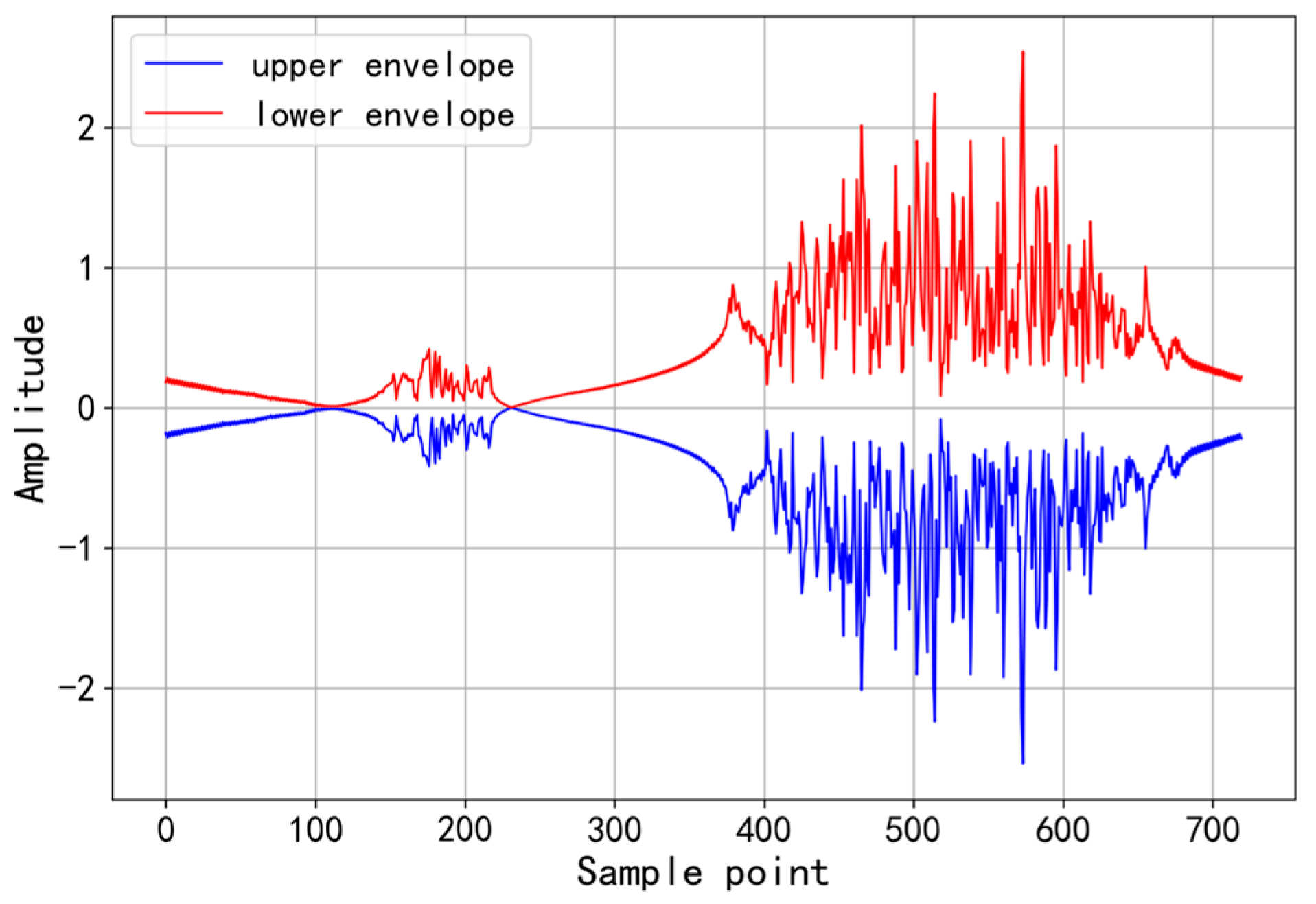
Envelope analysis was used to calculate and plot the upper and lower envelopes of the signal, further revealing the signal’s fluctuation amplitude and overall shape. This is crucial for noise removal and signal feature enhancement. As shown in Figure 5, the envelope plot reveals the concentration and intensity changes in the PD signal within specific phase intervals, which can help identify potential defect areas in the equipment.

3.1.2. The T-SNE Computation of the Extracted Features

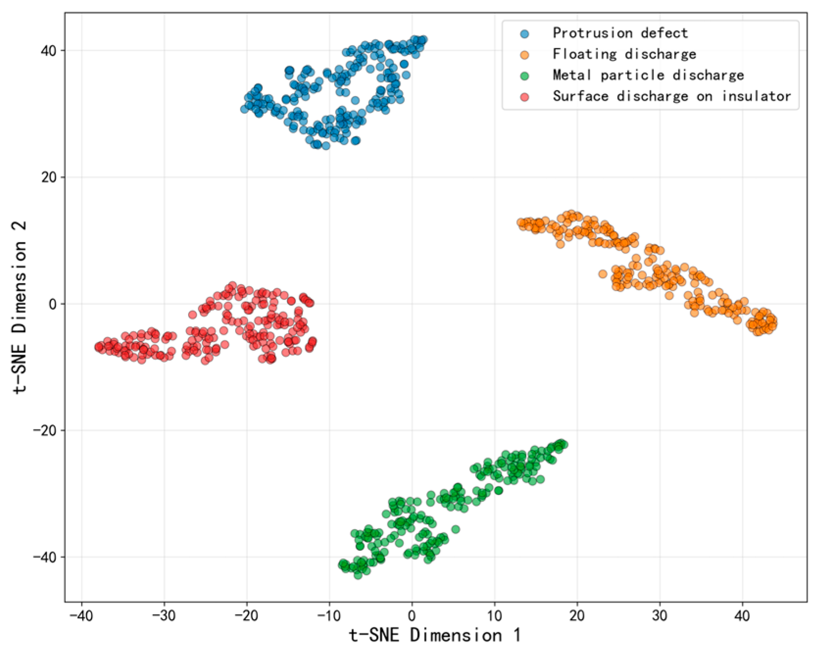
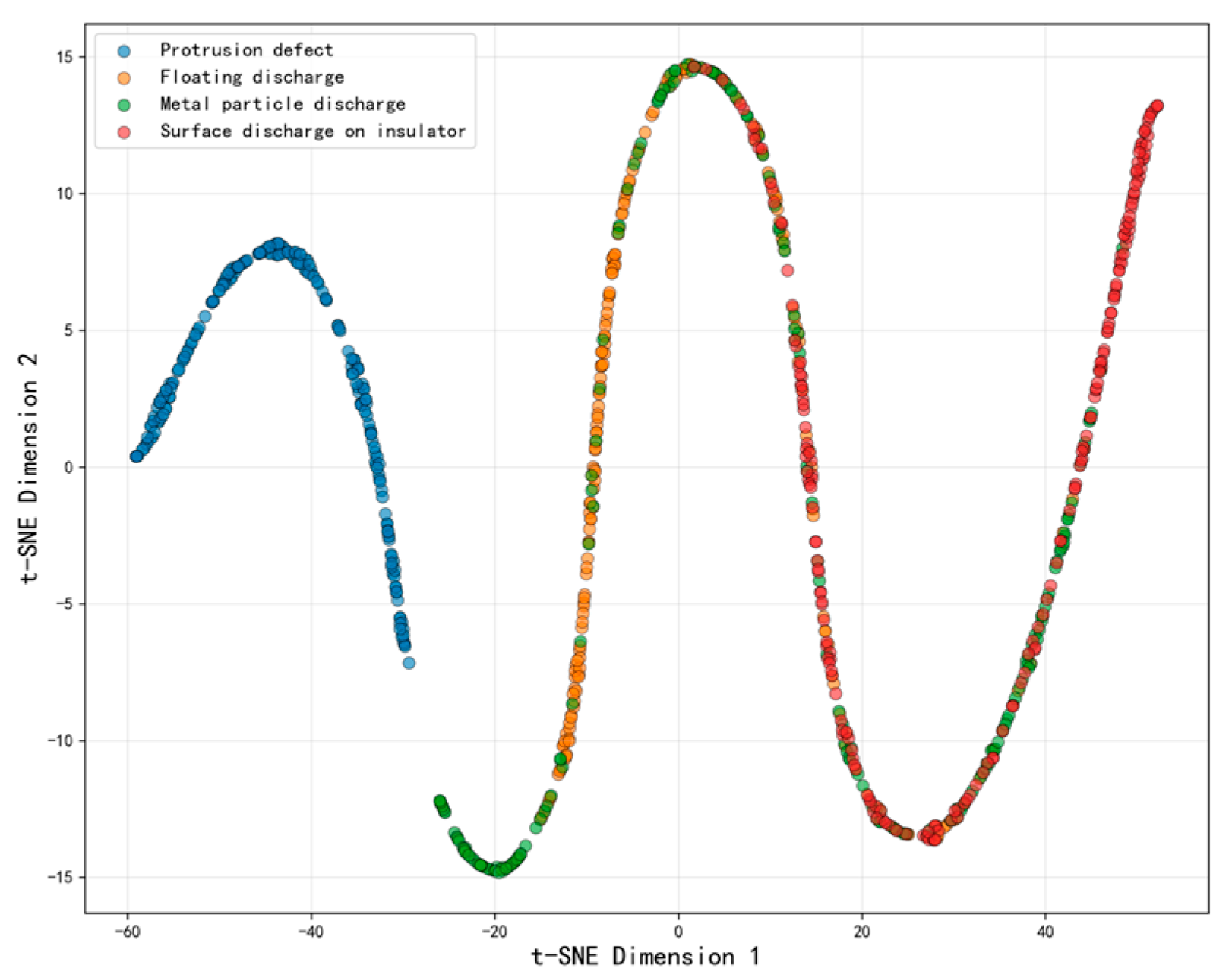
To verify the effectiveness of the extracted time-domain features in distinguishing different types of PD defects, this work uses the t-distributed Stochastic Neighbor Embedding (t-SNE) algorithm for dimensionality reduction and visualization. It preserves the local structure of the data, meaning that points that are close together in high-dimensional space will also be close together in the low-dimensional representation. The t-SNE algorithm was used to reduce the 8-dimensional feature vectors extracted from the PRPD samples to 2 dimensions, with the perplexity set to 30. The results are shown in Figure 6.

3.2. Signal Feature Extraction of UHF

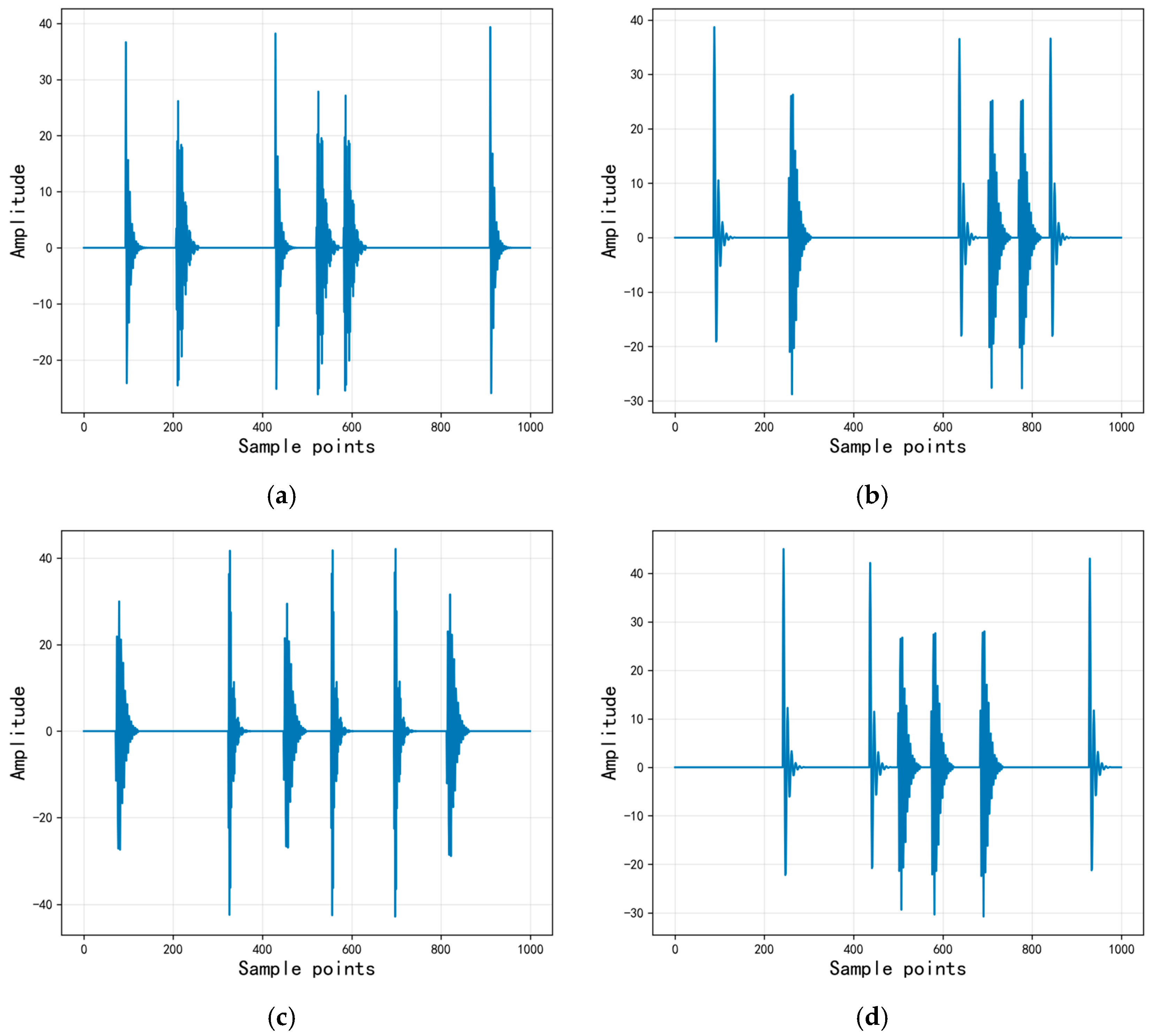
For UHF signals containing rich high-frequency components, frequency-domain analysis is an effective method to characterize the distribution of signal energy across different spectral bands, the collected signals of UHF are shown in Figure 7. This work uses Variational Mode Decomposition (VMD) on the raw time-domain signal to filter out noise interference [23]. VMD is an adaptive signal decomposition method that decomposes a complex signal into several Intrinsic Mode Functions (IMFs) with different center frequencies, separating the main physical components from high-frequency noise and irrelevant disturbances. Compared with traditional Empirical Mode Decomposition (EMD), VMD has better noise immunity and frequency separation capabilities. Its variational model can be expressed as:

$${\min }_{\left\{u_k\right\},\left\{{\omega }_k\right\}}\left\{{\displaystyle \sum _k{‖{\partial }_t\left[\left(\delta (t)+\frac{j}{\pi t}\right)*u_k(t)\right]e^{-j{\omega }_{k}t}‖}_2^2}\right\}\hspace{1em}\mathrm{s}.\mathrm{t}.{\displaystyle \sum _k{u}_k}=f$$

(9)

where u_k(t) denotes the k-th IMF, ω_k denotes the center frequency of the k-th mode, and f denotes the original input signal.

For the input signal f_t, VMD seeks K modal functions u_k(t) such that the sum of the estimated bandwidths of each mode is minimized, while satisfying the constraint that the sum of all modes equals the original signal. In this work, the number of decomposition modes is set to K = 10, decomposing the original signal into 10 IMF components from low frequency to high frequency; the bandwidth constraint parameter α = 2000 is used to control the bandwidth of each mode; and the convergence tolerance is 1 × 10⁻⁷.

The VMD algorithm requires two key parameters: the number of decomposition modes K and the bandwidth constraint parameter α. In this work, K was determined using a center frequency observation approach. We progressively increased K from 3 and examined the center frequencies of the resulting IMFs. When K exceeded 10, modes with similar center frequencies began to appear, indicating over-decomposition. Therefore, K = 10 was selected as the optimal value.

The bandwidth constraint parameter α controls the trade-off between frequency resolution and mode integrity. A larger α produces narrower bandwidth but risks mode splitting, while a smaller α may cause mode mixing. Through experimental comparison with α values ranging from 1000 to 3000, we found that α = 2000 provided the best balance for our UHF signals, yielding well-separated modes without significant energy leakage. The convergence tolerance was set to 1 × 10⁻⁷ to ensure sufficient iteration precision.

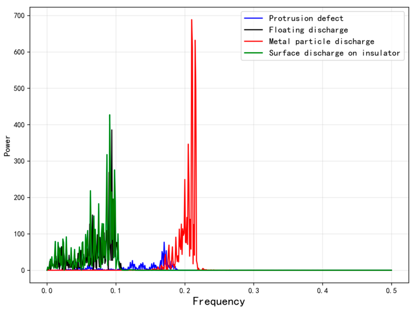
Figure 8 shows a comparison of the frequency-domain spectra of different signals, since the main energy of the UHF PD signal is concentrated in the low-frequency modes, and the high-frequency modes often contain more noise components, this work selects the first three modal components for superposition reconstruction to achieve signal denoising.

After denoising and reconstruction, the Power Spectral Density (PSD) of the processed signal is calculated to quantify the distribution of spectral energy. For a discrete signal x[n] of length N, its periodogram power spectral estimate is defined as Equation (10). PSD describes how the signal power changes with frequency, and therefore can serve as a concise representation of the differences in frequency response under different defect excitations.

$$P(f)={\displaystyle \frac{1}{N}}{\left|{\displaystyle \sum _{n=0}^{N-1}x}[n]e^{-j2\pi fn}\right|}^2$$

(10)

where P(f) denotes the power spectral density value at frequency f, N is the total number of samples, and x[n] denotes the amplitude of the n-th sampling point.

This work extracts six representative frequency-domain feature parameters based on the calculated PSD to characterize the frequency characteristics of ultra-high frequency PD signals.

Table 1. UHF signal frequency-domain feature parameters.

No.	Feature Name	Physical Significance
1	Mean spectral amplitude	Reflects the overall energy level of the power spectrum
2	Spectral centroid frequency	Indicates where the spectral energy is concentrated (first-order moment)
3	Mean square frequency	Reflects the dispersion of the spectral distribution (second-order moment)
4	Signal area	Power-spectrum shape feature based on the envelope
5	Average frequency	Weighted average frequency based on the power spectrum in dB
6	Mean power	Overall energy level on a logarithmic scale

summarizes the six UHF-domain feature parameters extracted in this work and their physical meanings.

The average frequency-domain amplitude reflects the overall energy level of the power spectrum and is defined by Equation (11), which is the arithmetic mean of the power spectrum at all frequency points.

$$A_{ve}={\displaystyle \frac{1}{M}}{\displaystyle \sum _{i=1}^{M}P}(f_i)$$

(11)

where A_ve denotes the average frequency-domain amplitude, M is the total number of frequency points, and P(f_i) is the power spectral density value at the i-th frequency point.

The centroid frequency represents the center of gravity of the power spectrum, reflecting the concentration trend of signal energy in the frequency domain. Its expression is:

$$C_F={\displaystyle \frac{{\displaystyle \sum _{i=1}^M{f}_i}\cdot P(f_i)}{{\displaystyle \sum _{i=1}^{M}P}(f_i)}}$$

(12)

where C_F denotes the centroid frequency, M is the total number of frequency points, and P(f_i) is the power spectral density value at the i-th frequency point.

Equation (13) represents the mean square frequency, which is the second moment of the spectrum, reflecting the degree of dispersion of the power spectrum distribution relative to the origin.

$$M_{SF}={\displaystyle \frac{{\displaystyle \sum _{i=1}^M{f}_i^2}\cdot P(f_i)}{{\displaystyle \sum _{i=1}^{M}P}(f_i)}}$$

(13)

where M_SF denotes the mean square frequency, M is the total number of frequency points, and P(f_i) is the power spectral density value at the i-th frequency point.

The signal area is calculated by computing the envelope of the power spectrum using the Hilbert transform, and then integrating the area between the upper and lower envelopes, reflecting the overall morphological characteristics of the power spectrum curve. Its expression is:

$$A_{rea}={\displaystyle \sum _{i=1}^M\left[E_{upper}(f_i)-E_{lower}(f_i)\right]}$$

(14)

where A_rea denotes the signal area, M is the total number of frequency points, and E_upper(f_i) and E_lower(f_i) represent the upper and lower envelope values of the power spectrum at frequency f_i.

The average frequency is calculated based on the decibel (dB) representation of the power spectrum, which can better reflect the contribution of low-energy frequency components. It first converts the power spectrum to decibel values and then calculates the frequency, as shown in Equations (15) and (16).

$$P_{dB}(f)=10\cdot {\log }_{10}[P(f)]$$

(15)

where P_dB(f) denotes the power spectral density in decibels at frequency f, and P(f) is power spectral density at frequency f.

$$M_f={\displaystyle \frac{{\displaystyle \sum _{i=1}^M{f}_i}\cdot P_{dB}(f_i)}{{\displaystyle \sum _{i=1}^M{P}_{dB}}(f_i)}}$$

(16)

where M_f denotes the mean frequency, M is the total number of frequency points, and P_dB(f_i) denotes power spectral density value in decibels at the i-th frequency point.

The average power is the arithmetic mean of the power spectrum decibel values, reflecting the overall energy level of the signal on a logarithmic scale. It is defined by the following formula:

$$M_p={\displaystyle \frac{1}{M}}{\displaystyle \sum _{i=1}^M{P}_{dB}}(f_i)$$

(17)

where M_p denotes the mean power, M is the total number of frequency points, and P_dB(f_i) denotes power spectral density value in decibels at the i-th frequency point.

Similar to Section 3.1.2 of this work, the t-SNE algorithm is used to reduce the 6-dimensional features of the UHF signal to 2 dimensions for visualization. As shown in Figure 9, the 6-dimensional features are reduced to 2 dimensions for visualization using t-SNE.

4. Multi-Feature Fusion and Dimensionality Reduction

4.1. Feature Normalization and Fusion

In this section, to exploit complementary information from the two sensing modalities, this work performs feature-level fusion by serially concatenating the extracted PRPD time-domain feature vectors and UHF-domain feature vectors. Specifically, the two sets of features are aligned sample by sample and then appended in the feature dimension to form an initial high-dimensional hybrid feature matrix. In this way, the PRPD features, which mainly characterize discharge phase–amplitude distribution and statistical patterns in the time domain, are combined with the UHF features, which reflect the spectral energy distribution and frequency-component characteristics of electromagnetic radiation signals. The resulting hybrid representation contains richer fault-discriminative information than single-modality features.

However, because the two modalities originate from different physical mechanisms and measurement systems, their feature components often differ markedly in physical meaning, units, and numerical scale. If these heterogeneous features are directly fed into a neural network, features with larger numerical scales tend to dominate the gradient updates, while small-scale features may be suppressed. This imbalance not only deteriorates the effective learning of the network but can also cause unstable training dynamics, slow convergence, or even failure to converge, ultimately degrading the robustness and accuracy of the classifier.

To address this issue, a normalization step is introduced prior to feature fusion. In particular, Z-score standardization is applied independently to each feature dimension across the training set. For a given feature x, the standardized value is computed as:

$${\widehat{x}}_{i,j}={\displaystyle \frac{x_{i,j}-{\mu }_j}{{\sigma }_j}}$$

(18)

where μ_j and σ_j denote the mean and standard deviation of j-th feature in the training set.

4.2. Feature Dimensionality Reduction Based on Principal Component Analysis (PCA)

Considering that the fused feature vector is formed by concatenating PRPD time-domain features and UHF-domain features, the overall dimensionality is significantly increased, and there may be strong correlations between different features, thus introducing potential multicollinearity problems. In this case, directly inputting the high-dimensional fused features into a classification model for training would, on the one hand, lead to parameter space expansion and reduced effective sample density, easily resulting in the curse of dimensionality, making it difficult for the model to learn stable and generalizable decision boundaries with limited samples; on the other hand, redundant features and noise components would interfere with the model’s extraction of key discriminative information, increasing the risk of overfitting, leading to good performance on the training set but degraded performance on the test set.

Therefore, this work introduces PCA after feature standardization to reduce the dimensionality of the fused feature matrix. PCA maps the original feature space to a set of mutually orthogonal new coordinate axes through linear transformation, so that the first few mapped directions can explain as much variance information in the data as possible. Specifically, the covariance matrix of the standardized feature matrix is first calculated and then subjected to eigenvalue decomposition to obtain the corresponding eigenvalues and eigenvectors. The eigenvalues reflect the amount of variance explained by each principal component, while the eigenvectors give the linear combination weights of the principal components in the original feature space. Subsequently, the principal components are sorted according to the magnitude of their eigenvalues, and based on the criterion that the cumulative variance contribution rate reaches a preset threshold, this work adopts a filtering strategy of eigenvalues greater than 0.001, finally selecting the first 9 principal components to construct a new low-dimensional feature representation as the input for the subsequent classifier. The number of principal components was determined by examining the cumulative explained variance ratio. The first 9 principal components collectively account for approximately 89.5% of the total variance in the fused feature set. Components beyond the 9th each contribute less than 0.1% to the total variance, primarily representing noise. Therefore, 9 principal components were retained, reducing the original 14-dimensional fused feature vector to a compact 9-dimensional representation suitable for classification.

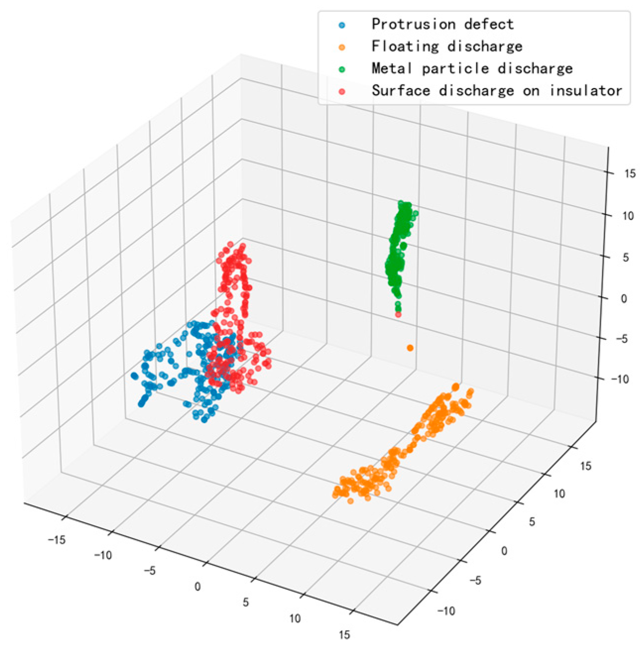
Through the above dimensionality reduction process, the fused features are effectively compressed while maintaining the main information structure: on the one hand, PCA retains the main variation patterns that contribute most to class differentiation, minimizing information loss; on the other hand, noise components and highly correlated redundant information in the original features are weakened or eliminated, thereby reducing the complexity of the input space and mitigating the adverse effects of multicollinearity on model training. Overall, this method provides a more compact, efficient, and robust input feature representation for subsequent classification models, which helps to improve training stability and generalization performance. The visualization of the multi-source fused features after PCA dimensionality reduction is presented in Figure 10.

5. A Fault Identification Model Based on ResNet-MLP

5.1. ResNet-MLP Network Architecture

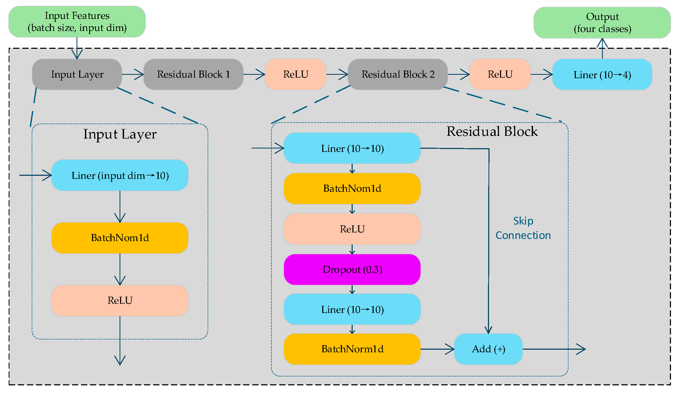
Traditional Multilayer Perceptrons (MLPs) suffer from slow convergence and unstable training when the network depth increases. Therefore, this work introduces the residual learning concept into a fully connected network, constructing a fully connected neural network classification model based on a residual structure (ResNet-MLP). The model structure is shown in Figure 11. It consists of three parts: first, an input mapping layer, which maps the feature vectors reduced by PCA to a unified hidden space dimension, and combines Batch Normalization and ReLU activation to stabilize feature distribution and enhance nonlinear expression; then, two serially stacked fully connected residual blocks are used to extract higher-level nonlinear discriminative features layer by layer; finally, a linear output layer maps the hidden space features to the class space of four fault types.

In each residual block structure, a main branch and identity skip connection is used, where the main branch consists of two fully connected layers, with Batch Normalization, ReLU activation, and Dropout (default dropout rate p = 0.3) introduced in between. For the k-th residual block, its main branch can be formally expressed as:

$$F(z)={\mathrm{BN}}_2\left(W_2\cdot \mathrm{Dropout}\left(\varphi \left({\mathrm{BN}}_1(W_{1}z+b_1)\right)\right)+b_2\right)$$

(19)

where F_(Z) denotes the mapping function of the main branch in the k-th residual block, Z is the input feature vector from the previous layer, W₁ and W₂ are the weight matrices of the two fully connected layers, ϕ(·) represents the ReLU activation function, BN denotes batch normalization, and Dropout is the regularization operation with dropout rate p.

The residual output is:

$$z^{\prime }=\varphi (z+F(z))$$

(20)

where F_(Z) denotes represents the main branch output computed by Equation (19), Z is the identity skip connection that directly passes the input to the output, and ϕ(·) represents the ReLU activation function.

In Figure 11, solid arrows represent the forward data flow, dashed lines enlarge the specific content contained in that layer, and different colors distinguish functional modules: orange represents liner layers, blue represents normalization, green represents activation functions, and purple represents dropout regularization. The “+” sign represents an add layer.

The core advantage of this structure lies in the fact that skip connections provide shorter gradient paths for backpropagation, allowing gradients to bypass some nonlinear transformations and be directly transmitted back to the shallower layers. This alleviates the optimization difficulties encountered during the training of deep MLPs, improving trainability while simultaneously enhancing the ability to express complex nonlinear feature mappings. Batch Normalization accelerates convergence and provides a certain degree of regularization by standardizing the input to each layer. The output layer uses a linear mapping and does not employ an activation function; it directly outputs logits for loss function calculation.

The ResNet-MLP model is configured with carefully tuned hyperparameters to balance model capacity and generalization ability. Considering that PCA dimensionality reduction only retains 9 features, a smaller hidden layer dimension is used to avoid overfitting.

Table 2. ResNet-MLP Model Hyperparameters.

No.	Hyperparameter	Value
1	Input dimension	9 (after PCA)
2	Hidden layer dimension	12
3	Number of residual blocks	2
4	Dropout rate	0.3
5	Batch size	64
6	Maximum epochs	150
7	Initial learning rate	0.003
8	Weight decay (L2 regularization)	1 × 10−3
9	Learning rate decay factor	0.5
10	LR scheduler patience	10 epochs
11	Early stopping patience	30 epochs
12	Output classes	4
13	Optimizer	AdamW
14	Loss function	Cross-Entropy

summarizes the key hyperparameters used in this study.

5.2. Training Process and Comparison of Results

After preliminary processing, there are 200 samples for each type of defect, resulting in a complete dataset of 800 samples. To ensure reliable evaluation and account for variability due to random data splitting, we performed 20 independent experimental runs with different random seeds. In each run, stratified random sampling was used to divide the data into training and test sets in an 8:2 ratio, ensuring a balanced distribution of each category across both sets. This resulted in 640 training samples and 160 test samples per run.

This work adopts the Cross-Entropy (CE) Loss function as the optimization objective during the model training phase. Internally, it first performs Softmax normalization on the model outputs, and then calculates the negative log-likelihood loss. Its expression is:

$$\mathcal{L}=-{\displaystyle \sum _{i=1}^C{y}_i}\log ({\widehat{y}}_i)$$

(21)

where $ℒ$ denotes the CE Loss, N is the total number of training samples, C is the number of classes (C = 4 in this work), and y_i is the ground-truth label indicator (1 if sample i belongs to class c, 0 otherwise).

This function quantifies the difference between the predicted class probability distribution and the true labels, and the model’s classification performance is gradually improved by minimizing this loss. Moreover, CE Loss imposes a more significant penalty on misclassifications, thus encouraging the model to learn more discriminative feature representations and decision boundaries.

For parameter updates, this work uses the AdamW optimizer for gradient optimization. AdamW retains the advantages of Adam’s adaptive learning rate and first- and second-order moment estimation, while decoupling weight decay from the gradient update process. This allows the regularization term to act on the parameter space in a more stable and controllable manner. This mechanism effectively suppresses unbounded parameter growth, reduces the effective complexity of the model, thereby improving training stability and enhancing the model’s generalization ability on unseen data.

To further improve the convergence efficiency and robustness of the training process, a dynamic learning rate scheduling strategy is introduced. Specifically, when the validation set loss does not show a significant decrease for several consecutive epochs, the learning rate is automatically decayed according to a preset rule. This allows for finer-grained parameter search and a smoother convergence trajectory in the later stages of training, avoiding oscillations or convergence stagnation caused by an excessively large learning rate.

Furthermore, considering that models are prone to overfitting under limited sample sizes, this work further adopts an early stopping mechanism as an effective regularization method: when the test set accuracy does not improve within the epoch interval corresponding to a preset patience value, the training process is terminated early, and the model parameters at the time of optimal performance are saved. This strategy effectively suppresses overfitting to the training data in the later stages, improving the stability and generalization performance of the final model, especially suitable for supervised learning tasks in small sample scenarios.

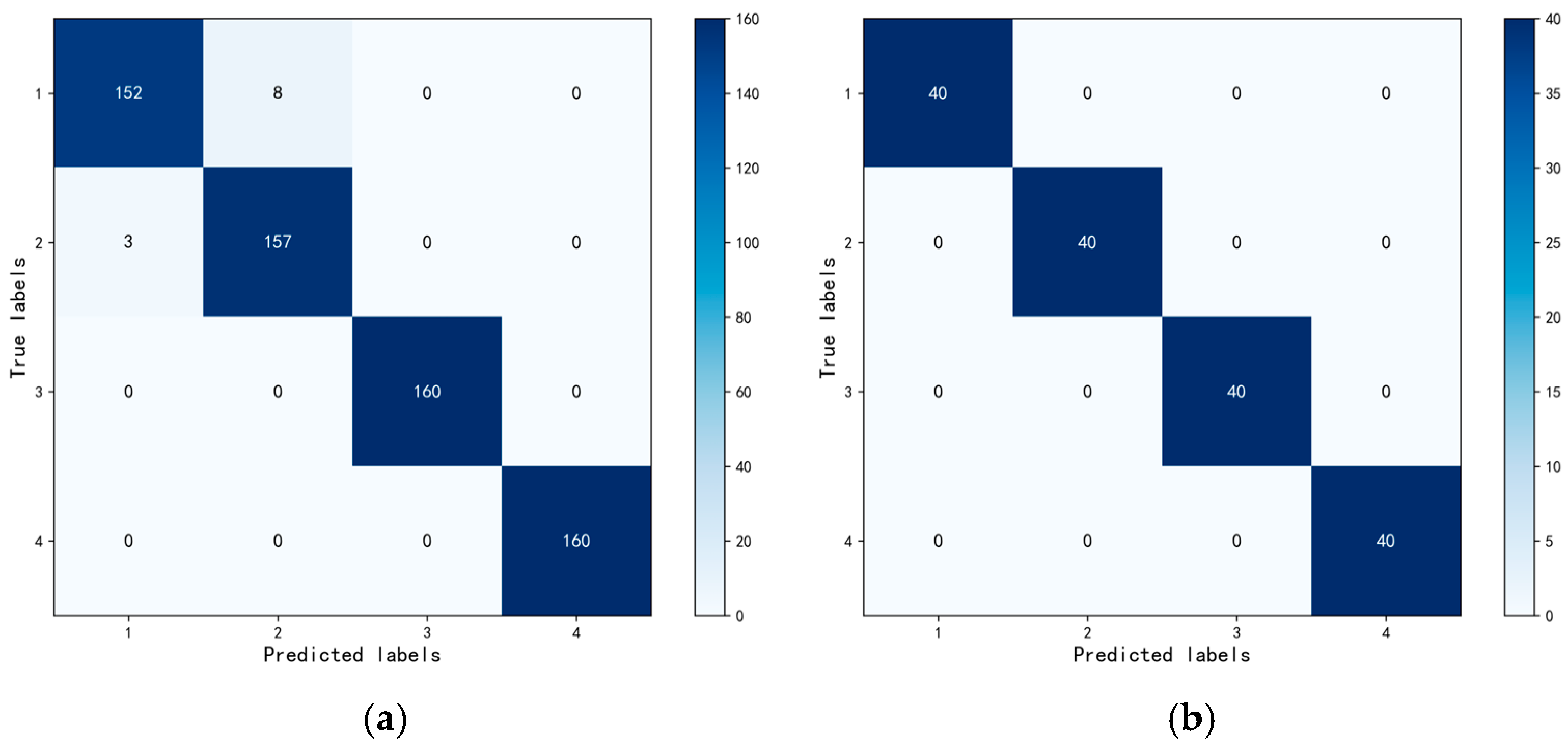
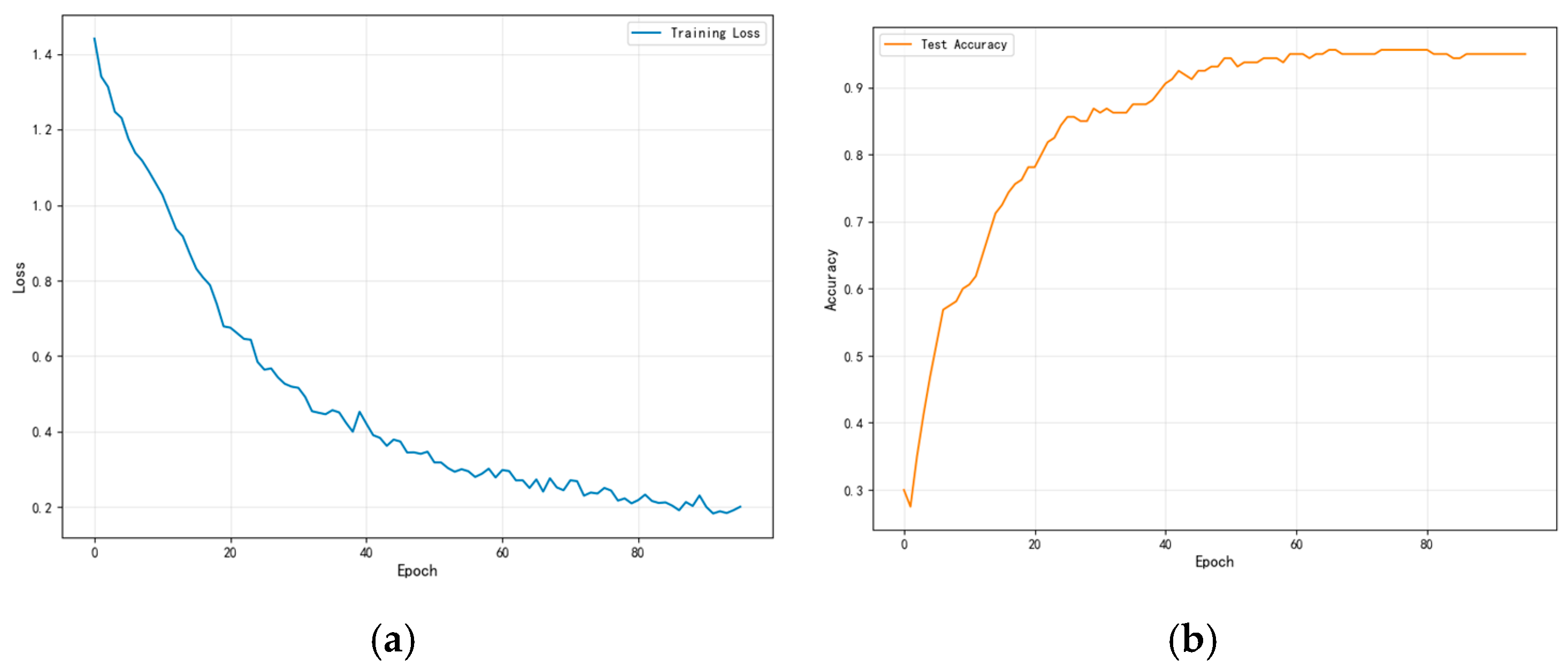
The confusion matrices of the training and test sets are shown in Figure 12. The training process exhibited stable convergence characteristics, as shown in Figure 13. The training loss decreased rapidly in the initial stages and gradually stabilized after approximately 50 epochs. The test accuracy also showed a corresponding upward trend, reaching its optimal value at approximately the 65th epoch. The early stopping mechanism was triggered at the 96th epoch when the test accuracy did not improve for 30 consecutive epochs, and the final test set accuracy reached 99.38%.

To comprehensively evaluate the classification performance of the proposed ResNet-MLP model, we report the precision, recall, and F1-score for each fault category on the test set, as summarized in

Table 3. Classification Performance on Test Set.

Defect Type	Precision (%)	Recall (%)	F1-Score (%)	Support
Protrusion defect	100.00	97.50	99.73	40
Floating discharge	97.56	100.00	98.77	40
Metal particle	100.00	100.00	100.00	40
Surface discharge	100.00	100.00	100.00	40
Overall Accuracy	/	/	99.38	160

. Overall Accuracy is the average of the values for the four types of defects and support indicates the number of true samples for each class in the test set.

To validate the effectiveness of the residual architecture, a comparative experiment was conducted between the proposed ResNet-MLP and a standard MLP baseline under identical conditions. The standard MLP with the only difference being the absence of skip connections. To ensure statistical reliability, both models were evaluated over 20 independent runs with different random seeds for data splitting.

Table 4. Comparison of ResNet-MLP and Standard MLP over 20 Independent Runs.

Model	Accuracy (%)	Precision (%)	Recall (%)	F1-Score (%)
Standard MLP	95.47 ± 3.72	96.78 ± 3.07	95.47 ± 3.72	94.79 ± 3.66
ResNet-MLP (Proposed)	98.94 ± 0.49	98.98 ± 0.46	98.94 ± 0.49	98.94 ± 0.49

summarizes the comparison results.

As shown in Table 4, the proposed ResNet-MLP achieves significantly higher performance than the standard MLP across all metrics. More importantly, the standard deviation of ResNet-MLP is substantially smaller, indicating more stable and reliable classification performance.

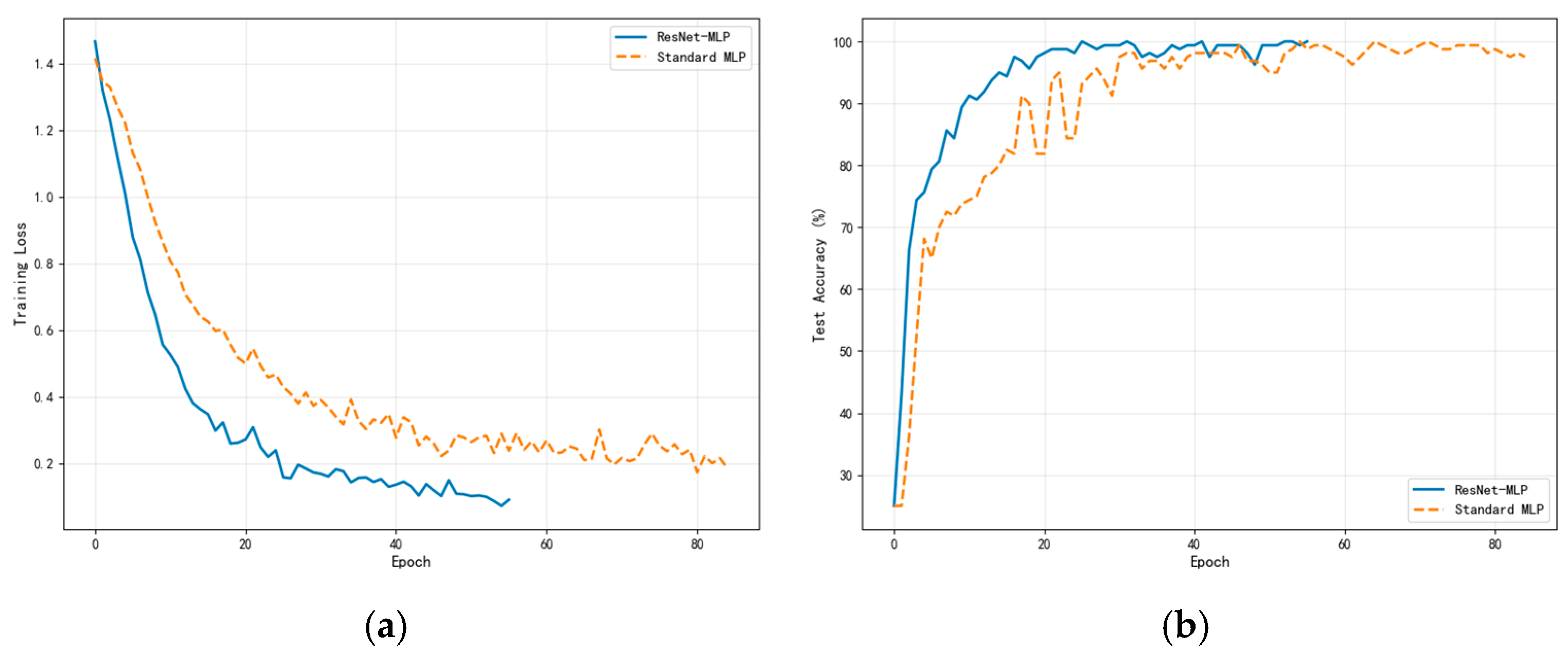
Figure 14 illustrates the training dynamics of both models under single train/test split conditions. Several key observations can be made. First, regarding convergence speed, ResNet-MLP converges faster, triggering early stopping at approximately epoch 55, while the standard MLP requires around 90 epochs. This demonstrates that skip connections facilitate more efficient gradient flow during backpropagation. Second, in terms of training stability, the loss curve of ResNet-MLP is smoother and more monotonically decreasing, whereas the standard MLP exhibits significant oscillations throughout training. Similarly, the test accuracy of ResNet-MLP stabilizes quickly at around 99%, while the standard MLP shows pronounced fluctuations between 60% and 100% before eventually stabilizing at approximately 96%. Third, considering final performance, ResNet-MLP achieves a lower final training loss (approximately 0.1) compared to the standard MLP (approximately 0.25), indicating better optimization of the network parameters.

These findings demonstrate that the residual connections effectively alleviate gradient-related optimization difficulties in the deeper network layers, enabling more stable training dynamics and superior classification performance. The skip connections provide shorter gradient paths during backpropagation, which helps maintain gradient magnitude and allows the network to learn more discriminative feature representations for GIS partial discharge fault diagnosis.

6. Conclusions

This work proposes a multi-modal PD fault diagnosis framework for GIS by fusing PRPD time-domain statistical features and UHF-domain features. After Z-score normalization, PCA is employed to obtain a compact low-dimensional representation, and a ResNet-MLP model is designed for defect classification.

Experiments conducted on four representative defect types—protrusion, floating discharge, metal particle, and insulator surface discharge—demonstrate that the proposed approach achieves 99.38% accuracy on the held-out test set, with consistently high precision, recall, and F1-score across all classes. These results validate the effectiveness of multi-modal feature fusion and the residual MLP architecture for nonlinear discrimination.

It should be noted that the current study was validated under laboratory conditions with well-defined defect types. In practical field applications, PD signals may contain higher noise levels and defect characteristics could partially overlap. However, the proposed method incorporates several design features that enhance its potential for field deployment. The VMD-based preprocessing provides effective noise suppression capability, while the multi-modal feature fusion combining HFCT and UHF measurements offers complementary information that improves robustness against single-sensor interference. Moreover, the consistently low variance of ResNet-MLP across 20 independent runs demonstrates strong generalization capability, suggesting potential resilience to real-world data variability. Future validation with field data from in-service GIS equipment will further confirm the practical applicability of the proposed approach.

Future work will focus on expanding the dataset to cover additional defect categories and operating conditions, validating the method on field data from in-service GIS, and exploring more robust feature-learning strategies to further enhance generalization and support online deployment. Additionally, the current experiments were conducted at a single voltage level (1.2 × inception voltage). Future work will include validation at multiple voltage levels to verify the robustness of the proposed method under varying operating conditions.

References

1. Li, C.; Zhang, C.; Lv, J.; Liang, F.; Liang, Z.; Fan, X.; Riechert, U.; Li, Z.; Liu, P.; Xue, J.; et al. China’s 10-Year Progress in DC Gas-Insulated Equipment: From Basic Research to Industry Perspective. iEnergy 2022, 1, 400–433. [Google Scholar] [CrossRef]
2. Song, X.; Shao, M. Health Assessment Method for Gas-Insulated Switchgear Based on Fault Tree Analysis. In Proceedings of the 2025 IEEE 3rd International Conference on Power Science and Technology (ICPST), Kunming, China, 16–18 May 2025; IEEE: New York, NY, USA, 2025; pp. 412–417. [Google Scholar]
3. Xing, Y.; Wang, Z.; Liu, L.; Xu, Y.; Yang, Y.; Liu, S.; Zhou, F.; He, S.; Li, C. Defects and Failure Types of Solid Insulation in Gas-insulated Switchgear: In Situ Study and Case Analysis. High Volt. 2022, 7, 158–164. [Google Scholar] [CrossRef]
4. Hussain, G.A.; Hassan, W.; Mahmood, F.; Shafiq, M.; Rehman, H.; Kay, J.A. Review on Partial Discharge Diagnostic Techniques for High Voltage Equipment in Power Systems. IEEE Access 2023, 11, 51382–51394. [Google Scholar] [CrossRef]
5. Yin, K.; Wang, Y.; Liu, S.; Li, P.; Xue, Y.; Li, B.; Dai, K. GIS Partial Discharge Pattern Recognition Based on Multi-Feature Information Fusion of PRPD Image. Symmetry 2022, 14, 2464. [Google Scholar] [CrossRef]
6. Liu, J.; Fan, X.; Zhang, C.; Lai, C.S.; Zhang, Y.; Zheng, H.; Lai, L.L.; Zhang, E. Moisture Diagnosis of Transformer Oil-Immersed Insulation with Intelligent Technique and Frequency-Domain Spectroscopy. IEEE Trans. Ind. Inform. 2021, 17, 4624–4634. [Google Scholar] [CrossRef]
7. Yang, J.; Hu, K.; Wang, F.; Zhang, J.; Bao, J.; Liu, W. A Partial Discharge Diagnosis Method for GIS Based on a Semi-Supervised Classification Framework and Density Peak Clustering Algorithm. IEEE Trans. Instrum. Meas. 2025, 74, 3516513. [Google Scholar] [CrossRef]
8. Álvarez, F.; Garnacho, F.; Ortego, J.; Sánchez-Urán, M. Application of HFCT and UHF Sensors in On-Line Partial Discharge Measurements for Insulation Diagnosis of High Voltage Equipment. Sensors 2015, 15, 7360–7387. [Google Scholar] [CrossRef]
9. Okabe, S.; Yamagiwa, T.; Okubo, H. Detection of Harmful Metallic Particles inside Gas Insulated Switchgear Using UHF Sensor. IEEE Trans. Dielectr. Electr. Insul. 2008, 15, 701–709. [Google Scholar] [CrossRef]
10. Gao, W.; Ding, D.; Liu, W. Research on the Typical Partial Discharge Using the UHF Detection Method for GIS. IEEE Trans. Power Deliv. 2011, 26, 2621–2629. [Google Scholar] [CrossRef]
11. Kong, F.; Zhao, K.; Ma, J.; Zhuang, T.; Li, H.; Gao, S.; Liu, J.; Zhang, C. Multiple Detections of Insulation Defects Partial Discharge in Gas-Insulated Equipment. Front. Energy Res. 2022, 10, 937599. [Google Scholar] [CrossRef]
12. Fang, W.; Chen, G.; Li, W.; Xu, M.; Xie, W.; Chen, C.; Wang, W.; Zhu, Y. A PRPD-Based UHF Filtering and Noise Reduction Algorithm for GIS Partial Discharge. Sensors 2023, 23, 6763. [Google Scholar] [CrossRef] [PubMed]
13. Meng, X.; Li, X.; Lu, T. Statistical Properties of Corona Current Pulses in Rod-Plane Air Gap Under AC–DC Composite Voltages. IEEE Trans. Dielectr. Electr. Insul. 2024, 31, 212–221. [Google Scholar] [CrossRef]
14. Hui, M.; Chan, J.C.; Saha, T.K.; Ekanayake, C. Pattern Recognition Techniques and Their Applications for Automatic Classification of Artificial Partial Discharge Sources. IEEE Trans. Dielectr. Electr. Insul. 2013, 20, 468–478. [Google Scholar] [CrossRef]
15. Hao, L.; Lewin, P. Partial Discharge Source Discrimination Using a Support Vector Machine. IEEE Trans. Dielectr. Electr. Insul. 2010, 17, 189–197. [Google Scholar] [CrossRef]
16. Hao, L.; Lewin, P.L.; Dodd, S.J. Comparison of Support Vector Machine Based Partial Discharge Identification Parameters. In Proceedings of the Conference Record of the 2006 IEEE International Symposium on Electrical Insulation, Toronto, ON, Canada, 11–14 June 2006; IEEE: New York, NY, USA, 2006; pp. 110–113. [Google Scholar]
17. Lei, Z.; Wang, F.; Li, C. A Denoising Method of Partial Discharge Signal Based on Improved SVD-VMD. IEEE Trans. Dielectr. Electr. Insul. 2023, 30, 2107–2116. [Google Scholar] [CrossRef]
18. Peng, X.; Yang, F.; Wang, G.; Wu, Y.; Li, L.; Li, Z.; Bhatti, A.A.; Zhou, C.; Hepburn, D.M.; Reid, A.J.; et al. A Convolutional Neural Network-Based Deep Learning Methodology for Recognition of Partial Discharge Patterns from High-Voltage Cables. IEEE Trans. Power Deliv. 2019, 34, 1460–1469. [Google Scholar] [CrossRef]
19. Zheng, J.; Chen, Z.; Wang, Q.; Qiang, H.; Xu, W. GIS Partial Discharge Pattern Recognition Based on Time-Frequency Features and Improved Convolutional Neural Network. Energies 2022, 15, 7372. [Google Scholar] [CrossRef]
20. Sun, W.; Ma, H.; Wang, S. A Novel Fault Diagnosis of GIS Partial Discharge Based on Improved Whale Optimization Algorithm. IEEE Access 2024, 12, 3315–3327. [Google Scholar] [CrossRef]
21. Srivastava, R.; Avasthi, V. Deep Convolutional Neural Network for Partial Discharge Monitoring System. Adv. Eng. Softw. 2023, 180, 103407. [Google Scholar] [CrossRef]
22. Greenacre, M.; Groenen, P.J.F.; Hastie, T.; Markos, A.; Tuzhilina, E. Principal Component Analysis. Princ. Compon. Anal. 2022, 2, 100. [Google Scholar] [CrossRef]
23. Dragomiretskiy, K.; Zosso, D. Variational Mode Decomposition. IEEE Trans. Signal Process. 2014, 62, 531–544. [Google Scholar] [CrossRef]
Figure 1. The schematic diagram of PD measurement setup.
Energies 19 01073 g001
Figure 2. Four fault models in GIS.
Energies 19 01073 g002
Figure 3. Photograph of the experimental setup: GIS test chamber with electrode configuration. This work connects the sensor output signal to a high-speed digital oscilloscope with a sampling rate of 5 GS/s. This configuration provides sufficient time resolution to capture fast transient electromagnetic pulses. The oscilloscope is synchronized with the applied voltage waveform through precise trigger settings, enabling PRPD correlation analysis. To ensure statistical significance, multiple measurements were performed under stable operating conditions, generating 200 sets of signal data for each defect type. After obtaining the raw signals, band-pass filtering was applied to the raw time-domain signals to suppress out-of-band noise and interference. Subsequently, frequency-domain features were extracted using spectral analysis techniques. PRPD analysis focuses on the phase-amplitude relationship, while UHF signal analysis focuses on the spectral energy distribution and frequency components, providing important complementary data for comprehensive fault diagnosis.
Energies 19 01073 g003
Figure 4. PRPD pattern of four fault types induced PD: (a) protrusion defect, (b) floating discharge, (c) metal particle discharge, and (d) surface discharge on insulator.
Energies 19 01073 g004
Figure 5. The results of extracting the upper and lower envelopes of the pulsed current signal.
Energies 19 01073 g005
Figure 6. Two-dimensional visualization of PRPD time-domain feature vectors using the t-SNE algorithm.
Energies 19 01073 g006
Figure 7. Collected signals of UHF: (a) protrusion defect, (b) floating discharge, (c) metal particle discharge, and (d) surface discharge on insulator.
Energies 19 01073 g007
Figure 8. Comparison of frequency-domain power spectra of UHF signals for different fault types.
Energies 19 01073 g008
Figure 9. Visualization of 6D frequency-domain features of UHF signals via t-SNE algorithm.
Energies 19 01073 g009
Figure 10. Three-dimensional visualization of multi-source fused features after PCA dimensionality reduction.
Energies 19 01073 g010
Figure 11. The architecture of the proposed ResNet-MLP network.
Energies 19 01073 g011
Figure 12. The confusion matrix of the proposed ResNet-MLP diagnostic model: (a) Confusion matrix of the training set and (b) Confusion matrix for the test set.
Energies 19 01073 g012
Figure 13. Convergence characteristics of the ResNet-MLP model: (a) Training loss curves and (b) test accuracy curves.
Energies 19 01073 g013
Figure 14. Comparison of training dynamics between ResNet-MLP and Standard MLP: (a) Training loss curves and (b) test accuracy curves.
Energies 19 01073 g014