Enhancing Oil Recovery in Ultra-Low Permeability Reservoirs Refracturing: Sweet Spot Evaluation and the Re-Pressurization Plus Infill-Fracturing Strategy

Abstract

The non-uniform production contribution caused by insufficient reservoir stimulation during initial fracturing significantly constrains the lifecycle and estimated ultimate recovery (EUR) of horizontal wells. Refracturing is therefore urgently required to reconstruct fracture networks and activate undeveloped reserves. In this study, a coupled geomechanics-matrix-fracture-seepage model is developed based on the Unconventional Fracturing Model (UFM) to characterize formation energy evolution and residual oil distribution. Simulation results indicate that initial fracturing creates a limited pressure diffusion radius (5–30 m), resulting in a “strong near-well, weak far-field” pressure distribution and inefficient residual oil utilization. To address this, a synergistic strategy is proposed, integrating “re-pressurization of existing fractures” for energy replenishment with “infill fracturing” for activating bypassed reserves. This strategy significantly outperforms conventional refracturing, increasing the predicted cumulative oil production by 55.86%. Parameter optimization indicates that maintaining a pumping rate of 10–12 m³/min and a fluid intensity of 1700–1900 m³/stage, while optimizing proppant ratios for conductivity, maximizes recovery. This work provides theoretical guidance for sweet spot evaluation and refracturing design in ultra-low permeability reservoirs.

1. Introduction

The low- to ultra-low permeability sandstone reservoirs in the central-southern Yishan Slope constitute significant hydrocarbon-bearing formations in the Ordos Basin, with lithologic reservoirs in the Yishan Slope and Paleozoic gas in the Tianhuan Depression being primary exploration targets. According to China’s 2023 Energy Assessment, the recoverable geological reserves of tight oil in the Ordos Basin are estimated at approximately 4.5–5.0 billion tonnes (including conventional ultra-low-permeability oil reservoirs and shale oil), accounting for 70–75% of the basin’s proven petroleum reserves. This region has become crucial for sustaining the stability of China’s onshore crude oil production [1,2]. These developed reservoirs exhibit significant burial depth variations. With ongoing exploration and development, two dominant resource types have emerged: Mesozoic oil reservoirs and Upper Paleozoic gas reservoirs, reflecting a multi-layered and multi-type resource distribution [3,4,5]. The reservoirs underwent prolonged shallow burial during the early stages and rapid deep burial in the later stages, resulting in uneven compaction and fluid expulsion, which readily leads to overpressure conditions. Based on field logging data from 25 wells in the block, the matrix porosity ranges from 8.5% to 11.5%. The relatively low geothermal gradient (approximately 2.5–3.0 °C/100 m) has delayed diagenesis, but has also exacerbated the development of overpressure, to some extent. As a result, these reservoirs exhibit typical “low porosity, low permeability, low pressure, and low abundance” characteristics. Effective and efficient production enhancement technologies are urgently needed to exploit the residual oil reserves [6].

In the early 1990s, North America pioneered the integration of horizontal drilling and hydraulic fracturing to successfully develop the Barnett Shale gas field, directly catalyzing the United States’ transition from a net energy importer to exporter. Subsequently, the concept of “hydraulic isolation” gradually emerged, with the application of hydraulic jetting and staged fracturing techniques [7,8,9,10,11,12]. In the early 2000s, China initiated the application of horizontal well fracturing technologies, with field trials conducted in tight and shale oil and gas formations in the Junggar, Sichuan, and Ordos Basins. These techniques achieved effective development of large quantities of oil and gas reservoirs that are difficult to exploit due to low economic returns from vertical well fracturing, such as low-permeability, ultra-low-permeability, and tight sandstones, oil shales, and ultra-deep carbonate rocks [13,14,15,16]. For wells experiencing post-initial-fracturing or natural production decline, refracturing treatments or infill drilling around parent wells are standard industry practices to restore or enhance production. These constitute core re-stimulation techniques for sustaining unconventional resource development [17,18]. However, complex fracture networks created during initial stimulation are prone to channeling during flooding, exacerbating reservoir heterogeneity and energy depletion. Consequently, residual oil exhibits coexisting dispersed and locally concentrated distribution patterns. According to production evaluations by oilfield service companies in North American shale refracturing operations, over 40% of perforation clusters contribute little to no output, due to insufficient stimulation or uneven proppant placement [19]. This inefficiency results in a specific distribution pattern of residual oil: while near-fracture zones are depleted, substantial “bypassed oil” remains trapped in the unstimulated regions between valid stages. An analysis of 22 fractured horizontal wells in the tight gas reservoirs of the eastern Ordos Basin revealed that only 30% of the fractured stages contributed to over 90% of the total production, with the remaining stages deemed ineffective due to poor sweet spot connectivity [20]. Therefore, simply re-fracturing existing perforations cannot effectively tap into these inter-stage reserves. A strategy combining energy replenishment in old fractures with the creation of new infill fractures is required. However, current numerical studies rarely quantify the complex geomechanical interference between re-pressurized old fractures and propagating new infill fractures. Existing optimization research often treats these mechanisms in isolation, failing to capture the dynamic evolution of the seepage field during this coupled process.

This extreme imbalance in production contribution shows the urgent need for precise modeling and characterization of hydraulic fractures to optimize development strategies and enhance recovery in unconventional reservoirs. The Unconventional Fracture Model (UFM) was developed specifically for naturally fractured formations, enabling the simulation of fracture propagation at multiple tips [21,22]. Kresse et al. proposed a semi-analytical fracture modeling platform based on the accuracy of the Displacement Discontinuity Method (DDM), which investigated the effects of friction coefficient, fracture propagation direction, and in situ stress on hydraulic–natural fracture interaction [23]. The Extended Finite Element Method (XFEM) was utilized to simulate hydraulic–natural fracture interactions without the need for remeshing, thereby enabling accurate modeling in heterogeneous reservoirs with complex boundary conditions [24]. Field demonstrations and recent theoretical investigations confirm that accurate characterization of hydraulic-fracture geometry, dynamic simulation of formation energy fields—specifically the stress evolution induced by pressure depletion—and spatial mapping of bypassed reserves, are critical for reliable reservoir performance prediction and the optimization of subsequent refracturing and infill well development [25,26,27,28,29].

Accurate evaluation of residual oil distribution and sweet spot potential in ultra-low permeability reservoirs is important for optimizing development strategies, risk mitigation, and enhanced oil recovery. To bridge the gap between static geological characterization and dynamic fracture propagation in refracturing design, this study develops a fully coupled geomechanics-matrix–fracture-seepage model, based on the updated UFM framework. Distinct from previous preliminary studies or single-factor analyses, this work introduces a novel quantitative sweet spot evaluation method specifically calibrated for ultra-low permeability reservoirs. Furthermore, we propose and rigorously validate a “synergistic strategy” that integrates re-pressurization of depleted zones with infill fracturing. This approach explicitly addresses the formation energy deficit—a critical factor often overlooked in conventional refracturing optimizations—providing a robust pathway to maximize the estimated ultimate recovery (EUR).

2. Model Establishment

To quantify the impact of geological and engineering factors on horizontal well fracturing in ultra-low permeability reservoirs, a comprehensive model is required to capture the significant changes in seepage and stress fields during late-stage waterflooding. A geomechanics-matrix–fracture-seepage coupling model is constructed, incorporating the fluid–solid dynamic coupling between the matrix and fractures under reservoir conditions, and the influence of proppant transport on the final conductivity of hydraulic fractures. In addition, the updated stress field (including stress shadow effects) from the hydraulic fracturing simulator is iteratively fed back into the geomechanical model to constrain subsequent fracture propagation and conductivity evolution. To ensure computational efficiency and accuracy, fracture propagation is simulated using the Petrel–Kinetix hydraulic fracturing platform. This simulation integrates the Schlumberger Petrel™ platform (V2021, Schlumberger, Houston, TX, USA) for static geological modeling with the Kinetix™ simulator (V2017, Schlumberger, Houston, TX, USA) for dynamic hydraulic fracturing, coupled via a bi-directional data exchange interface. The UFM models fluid–reservoir interactions during fracture growth. Distinct from conventional 3D modeling, this workflow features strongly nonlinear, multi-physics, multi-timestep, and multi-scale coupling characteristics, necessitating advanced equation-solving methodologies [30,31,32].

2.1. Theoretical Framework and Governing Equations

When simulating fracture propagation in multi-layered formations using the UFM model, fracture geometry is primarily governed by fluid pressure, in situ stresses, fracture toughness, layer thickness, and elastic modulus. Accordingly, key assumptions for the fracture propagation model include the following: (a) each cross-section is independent, and plane strain conditions are assumed; (b) the fracture is assumed to be a vertical planar fracture, discretized along its length into segments of varying heights, which may span multiple thin layers; and (c) fluid flow occurs horizontally along the fracture length, with vertical flow and pressure gradients neglected except near the fracture tips and boundaries. The pressure distribution within the fracture cross-section can be expressed as:

$$p=p_{cp}+{\rho }_{f}g\left(h_{cp}-l\right)$$

(1)

where $p_{cp}$ is fracture pressure at depth $h_{cp}$. $l$ is position along fracture, and ${\rho }_f$ is fluid density. Under the assumption of equilibrium height, the stress intensity factors at the top and bottom tips of the fracture can be determined, based on the internal fracture pressure, fracture geometry, and in situ stress. For asymmetric multi-layer solutions, the governing relations are expressed as:

$$\begin{array}{l}{K}_{IU}=\sqrt{\frac{\pi h}{2}}\left[p_{cp}-{\sigma }_n+{\rho }_{f}g\left(h_{cp}-{\displaystyle \frac{3}{4}}h\right)\right]+\sqrt{\frac{2}{\pi h}}{\displaystyle \sum _{i-1}^{n-1}}({\sigma }_{i+1}-{\sigma }_i)\left[{\displaystyle \frac{h}{2}}arccos\left({\displaystyle \frac{h-2h_i}{h}}\right)-\sqrt{h_i(h-h_i)}\right]\\ \end{array}$$

(2)

$$\begin{array}{l}{K}_{IL}=\sqrt{{\displaystyle \frac{\pi h}{2}}}\left[p_{cp}-{\sigma }_n+{\rho }_{f}g\left(h_{cp}-{\displaystyle \frac{h}{4}}\right)\right]+\sqrt{{\displaystyle \frac{2}{\pi h}}}{\displaystyle \sum _{i-1}^{n-1}}({\sigma }_{i+1}-{\sigma }_i)\left[{\displaystyle \frac{h}{2}}arccos\left({\displaystyle \frac{h-2h_i}{h}}\right)-\sqrt{h_i(h-h_i)}\right]\\ \end{array}$$

(3)

where $K_{IU}$ and $K_{IL}$ are the stress intensity factors at the top and bottom tips of the vertical fracture $K_{IU}$. $h$ is the fracture height. $h_{cp}$ is the height from the perforation location to the bottom tip of the fracture. ${\sigma }_n$ is the normal stress, MPa. $i$ is the layer index ranging from the top to the bottom of the fracture. $h_i$ is the vertical distance from the top of the $i$ layer to the bottom tip of the fracture.

While describing fluid flow, mass conservation, and fracture deformation in fracture networks, both the UFM Model and Pseudo-3D models are fundamentally based on classical Linear Elastic Fracture Mechanics (LEFM) and lubrication theory [33] frameworks. Therefore, Poiseuille’s law governs the flow equation for power-law fluids within fractures:

$$\begin{array}{l}{\displaystyle \frac{\partial p}{\partial s}}=-{\alpha }_0{\displaystyle \frac{1}{{\overline{w}}^{2n^{\prime }+1}}}{\displaystyle \frac{q}{H_{fl}}}{\left|{\displaystyle \frac{q}{H_{fl}}}\right|}^{n^{\prime }-1}\\ {\alpha }_0={\displaystyle \frac{2K}{\mathsf{\Phi }{\left(n^{\prime }\right)}^{n^{\prime }}}}{\left({\displaystyle \frac{4n^{\prime }+2}{n^{\prime }}}\right)}^{n^{\prime }}\\ \mathsf{\Phi }\left(n^{\prime }\right)={\displaystyle \frac{1}{H_{fl}}}{\displaystyle \underset{H_{fl}}{\int }}{\left({\displaystyle \frac{w\left(z\right)}{\overline{w}}}\right)}^{{\displaystyle \frac{2n^{\prime }+1}{n^{\prime }}}}dz\end{array}$$

(4)

where $p$ is the fluid pressure. $s$ is the flow distance along the fracture. $q$ represents the fluid velocity in the fracture. $H_{fl}$ is the height of the fluid within the fracture. $w(z)$ is the fracture width at depth $z$. $\overline{w}$ is the average fracture width. $n^{\prime }$ and $K$ are the flow behavior index and consistency index of the power-law fluid, respectively.

Within a fracture element, the local mass conservation of the fluid is governed by the continuity (mass balance) equation, expressed as:

$$\begin{array}{l}{\displaystyle \frac{\partial q}{\partial s}}+{\displaystyle \frac{\partial \left(H_{fl}\overline{w}\right)}{\partial t}}+q_l=0\\ q_l={\displaystyle \frac{2h_l{C}_t}{\sqrt{t-\tau \left(s\right)}}}\\ t>{\tau }_0\left(s\right)\end{array}$$

(5)

where $q_l$ is the leak-off rate of fracturing fluid into the formation. $h_l$ is the height of the invaded (leak-off) zone. $C_t$ is the total leak-off coefficient. ${\tau }_0(s)$ denotes the time when fluid first enters a specific fracture element. Additionally, global volume conservation must be satisfied:

$${\displaystyle {\int }_0^{t}Q\left(t\right)}dt={\displaystyle \underset{H_{fl}}{\int }{\displaystyle {\int }_0^{L\left(t\right)}{\displaystyle {\int }_0^t{q}_L}}}dtdsdh$$

(6)

where $Q\left(t\right)$ is the dynamic injection rate. $L(t)$ is the total length of all fractures at time $t$. $H\left(s,t\right)$ represents the fracture height.

Injected fluid in the wellbore must either enter fractures or leak off into the surrounding formation; thus, the total injection rate equals the sum of instantaneous perforation cluster rates during initiation [22,34], expressed as:

$$\begin{array}{l}{\displaystyle \sum _i}{q}_i\left(t\right)=Q\left(t\right)\\ i=1\dots N_{perf}\end{array}$$

(7)

where $q_i\left(t\right)$ is the flow rate for each perforation cluster.

2.2. Proppant Transport Model

In this study, a one-dimensional proppant transport model is employed in the horizontal direction to calculate the migration of various fluids and proppants in the fracture network, taking into account multiple factors including advective transport, fluid leak-off, proppant bridging, deposition, gravitational settling, and proppant bank erosion. Based on the transport equations of proppant, the vertical heights of the proppant bank, mud, and fracturing fluid in each fracture element at every time step are calculated. The integral formulation for fluid phase concentrations above the proppant bank (pure fluid zone) is given as:

$$C_k={\displaystyle \frac{1}{\Delta x^{\prime }\overline{w\left(H-H_{bank}\right)}}}{\displaystyle \underset{H_{bank}}{\overset{H}{\int }}}{\displaystyle \underset{-{\displaystyle \frac{\overline{w}}{2}}}{\overset{{\displaystyle \frac{\overline{w}}{2}}}{\int }}}{\displaystyle \underset{x_c^{\prime }-{\displaystyle \frac{\Delta x}{2}}}{\overset{x_c^{\prime }+{\displaystyle \frac{\Delta x}{2}}}{\int }}}{X}_k\left(x^{\prime },y^{\prime },z\right)d{x}^{\prime }d{y}^{\prime }dz$$

(8)

where $C_k$ is the proppant concentration. $\Delta x^{\prime }$ is the length of the fracture element. $H_{bank}$ is the proppant bank height. $X_k$ is the volumetric fraction of phase $k$.

The one-dimensional proppant transport equation used in this study is similar to the formulation presented by Clark and Adachi [35,36], but differs in assuming purely advective transport for both proppant and fluid within fractures. For the fluid phase, the leak-off mass is modeled as a source term in the transport equation as:

$${\displaystyle \frac{\partial \left(H-H_{\mathit{bank}}\right)\overline{w}{c}_{fl,k}}{\partial t}}+{\displaystyle \frac{\partial \left(q_{fl}{c}_{fl,k}\right)}{\partial x}}+f_{lea{k}_{off}}{c}_{fl,k}=0$$

(9)

where $q_{fl}$ the fluid velocity. $f_{lea{k}_{off}}$ is the wall-normal fluid flow rate above the proppant bank, which also represents fluid leak-off through the fracture walls in the vertical direction.

Vertically, the proppant transport model incorporates two competing mechanisms: proppant settling into the proppant bank and erosion of the deposited proppant. When the fracture width is insufficient for proppant passage, the model accounts for bridging effects, while erosion dynamics under localized velocity surges are also modeled. To address the assumption of homogeneity, the model incorporates a corrected settling velocity based on Stokes’ law [37], modified for fracture wall retardation effects and non-Newtonian fluid rheology:

$$v_{set,k}={\left[{\displaystyle \frac{1}{3^{\overline{n}-1}18}}{\displaystyle \frac{\left({\rho }_{\mathit{prop},\mathit{k}}-{\overline{\rho }}_{fl}\right)g}{{\overline{K}}^{\prime }}}{D}_k^{\overline{n}+1}\right]}^{{\displaystyle \frac{1}{\overline{n}}}}$$

(10)

where $v_{set,k}$ is the proppant settling velocity. ${\rho }_{\mathit{prop},\mathit{k}}$ is the density of the proppant. $D_k$ is the diameter of the proppant particles. $K^{\prime }$ and $n$ are the average consistency index and the average flow behavior index of the fluid, respectively, both weighted by fluid concentration.

2.3. Multi-Fracture Propagation Model

The Displacement Discontinuity Method (DDM) is employed to simultaneously solve the deformation of both the rock matrix and fractures, as well as fluid diffusion from fractures into the surrounding formation. For a linear elastic medium, the spatial distribution of stress and displacement can be expressed as:

$$\begin{array}{c}{\sigma }_{ij}=\lambda u_{k,k}{\delta }_{ij}+\mu \left(u_{i,j}+u_{j,i}\right)\\ \mu ={\displaystyle \frac{E\left(1+v\right)}{2}}\\ \lambda ={\displaystyle \frac{Ev}{\left(1+v\right)\left(1-2v\right)}}\end{array}$$

(11)

where ${\sigma }_{ij}$ represents the stress components in each direction. $E$ is the Young’s modulus of the material. The fracture surface divides the domain into an upper and a lower half-space. Across the fracture surface, a discontinuity in displacement occurs, while displacement remains continuous in regions outside the fracture ($\left|x\right|>a$, $y=0$ and $y\ne 0$).

In the upper half-space, the displacement field is related to the tangential and normal displacement discontinuities across the fracture elements, as follows:

$$\begin{array}{l}{u}_x=D_s\left[2(1-v)f_{,y}-y{f}_{,xx}\right]-D_n\left[(1-2v)f_{,x}+y{f}_{,xy}\right]\hfill \\ u_y=D_s\left[(1-2v)f_{,x}-y{f}_{,xy}\right]+D_n\left[2(1-v)f_{,y}-y{f}_{,yy}\right]\hfill \end{array}$$

(12)

The stress relationship can be expressed as:

$$\begin{array}{l}{\sigma }_{xx}=2G{D}_s\left[2f_{xy}+y{f}_{xyy}\right]+2G{D}_n\left[f_{,yy}+y{f}_{,yyy}\right]\hfill \\ {\sigma }_{yy}=2G{D}_s\left[-y{f}_{xyy}\right]+2G{D}_n\left[f_{yy}-y{f}_{,yy}\right]\hfill \\ {\tau }_{xy}=2G{D}_s\left[2f_{,yy}+y{f}_{,yy}\right]+2G{D}_n\left[-y{f}_{,xyy}\right]\hfill \end{array}$$

(13)

where $u_x$ is the displacement in the x-direction, and $u_y$ is the displacement in the y-direction. $D_s$ denotes the tangential displacement discontinuity across the fracture element. $D_n$ is the normal displacement discontinuity, with negative values indicating fracture opening.

To account for stress interaction among adjacent fractures in complex-fracture networks, three-dimensional correction factors are introduced. And a fracture-induced stress field model is established to quantify stress shadowing effects. The normal stress ${\sigma }_n$ and shear stress ${\sigma }_s$ acting on any fracture element are computed as the superposition of stresses induced by the tensile $D_n$ and $D_s$ shear $i$ displacement discontinuities of all other fracture elements, as:

$$\begin{array}{l}{\sigma }_n^i={\displaystyle \sum _{j=1}^N}{A}^{ij}{C}_{ns}^{ij}{D}_S^j+{\displaystyle \sum _{j=1}^N}{A}^{ij}{C}_{nn}^{ij}{D}_n^j\\ {\sigma }_S^i={\displaystyle \sum _{j=1}^N}{A}^{ij}{C}_{ss}^{ij}{D}_S^j+{\displaystyle \sum _{j=1}^N}{A}^{ij}{C}_{sn}^{ij}{D}_n^j\end{array}$$

(14)

where $C^{ij}$ denotes the two dimensional plane-strain elastic influence factor. $A^{ij}$ is the three-dimensional correction factor accounting for out-of-plane effects in fracture interactions.

The mechanism of such stress interaction is fundamentally governed by two coupled effects: mechanical stress interference and poroelastic response. Mechanically, the opening of hydraulic fractures exerts compressive stress on the surrounding rock (stress shadowing), altering the local principal stress magnitudes and reorienting the stress field. Simultaneously, fracturing fluid leak-off increases the pore pressure in the matrix, which induces poroelastic stress changes that further modify the effective stress distribution around the fractures. This dynamic evolution of the stress field creates the “perturbation” necessary to activate natural fractures and rebalance the energy field.

To align the simulation with field implementation constraints, the impact of effective stress increase on fracture conductivity is rigorously considered. Specifically, proppant embedment and long-term conductivity degradation are quantified using an exponential decay function dependent on the closure stress:

$$C_f=C_0{e}^{-d\Delta \sigma }$$

(15)

where $C_f$ is the current fracture conductivity, $C_0$ is the initial conductivity, $d$ is the degradation coefficient, and $\Delta \sigma$ represents the effective stress variation. This adjustment ensures that the EUR predictions account for the realistic decline in flow capacity during the production lifecycle.

2.4. Spatial Discretization and Numerical Solution

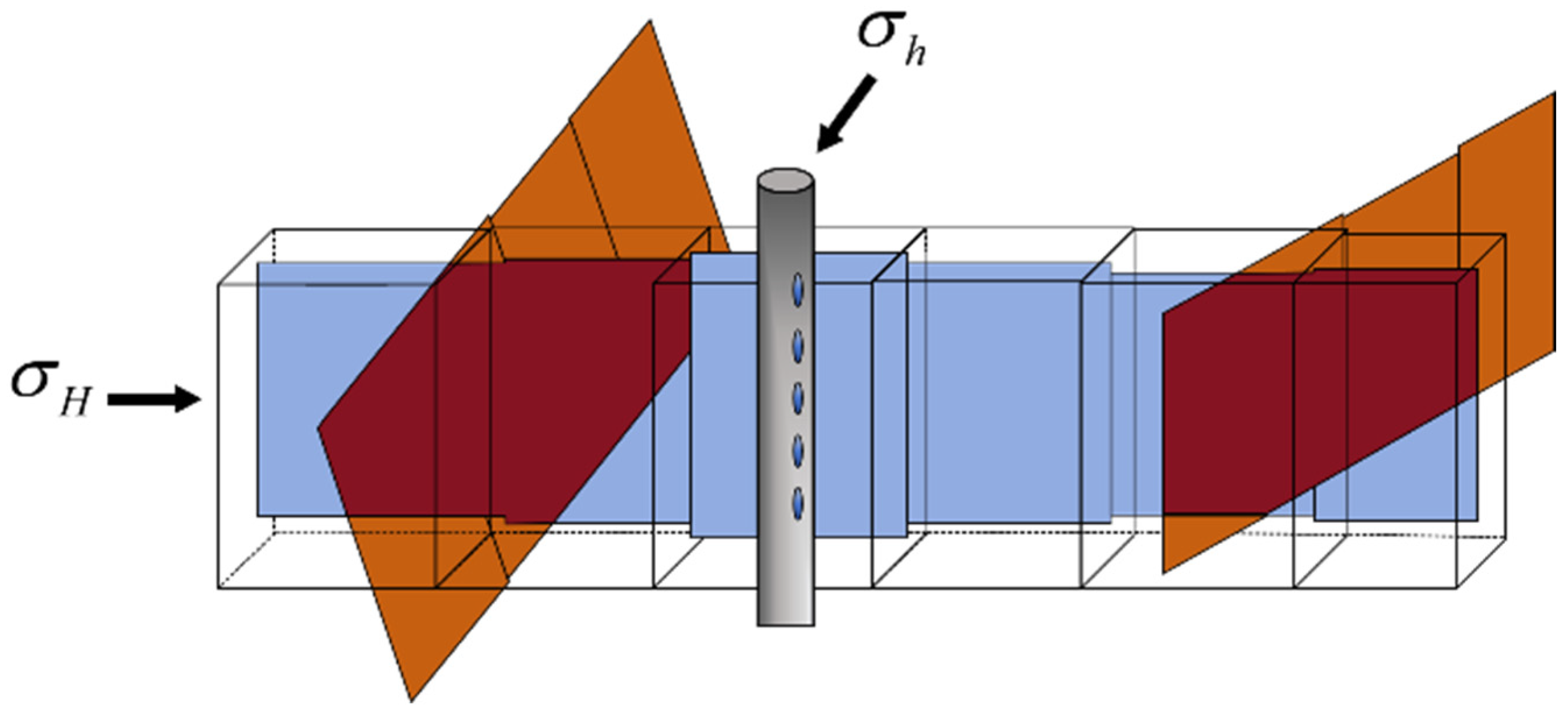
The discrete fracture network (DFN) representing natural fractures is generated based on Formation Microresistivity Imaging (FMI) logging data and ant-tracking seismic attributes, following a fractal length distribution. The UFM explicitly characterizes propagation and interaction of discrete fracture networks, while coupling stress fields to compute deformations. For fluid flow simulations, UFM employs unstructured meshes or specialized algorithms to explicitly resolve fracture networks and their branches, calculating interconnectivity between fracture elements (e.g., branch intersections, fracture–matrix connections) to model complex seepage pathways (Figure 1). The simulation domain employs no-flow boundary conditions to represent a symmetric sector model of the well pad, ensuring computational efficiency while capturing inter-well interference.

The conductivity is calculated using the method proposed by Karimi based on the Star–Delta transformation, and can be written as:

$$T_{nnc}={\displaystyle \frac{K_f{A}_{eff}}{d_{eff}}}$$

(16)

where $T_{nnc}$ is the conductivity. $K_f$ is the fracture permeability. $A_{eff}$ represents the effective contact area. $d_{eff}$ is the effective flow path length. When two fractures intersect, fluid exchange occurs at the intersection. Although the conductivity at the intersection can be determined using the harmonic or geometric mean of the conductivities of the two fractures, a more common method is to directly compute it based on the contact area and flow distance at the intersection, as:

$$T_{cross}=={\displaystyle {\sum }_{i=1}^n\frac{K_{f,i}{w}_i{L}_i}{d_{i,cross}}}$$

(17)

where $w_i$ is the width of the $i$-the fracture. $L_i$ denotes the length of the intersection segment and $d_i$ is the distance from the fracture element centroid to the intersection point.

The validity of the fluid–solid coupling assumptions within the UFM framework has been extensively verified against classic analytical solutions and experimental data in previous studies [38]. To further ensure the reliability of this study’s specific model, we conducted a sensitivity analysis on key geomechanical parameters (Young’s modulus and Poisson’s ratio). The fracture propagation geometry simulated by our model shows a deviation of less than 5% when compared to the standard KGD analytical solution under homogeneous conditions, confirming the numerical stability of the coupling algorithm [39]. The fluid–structure interaction simulation is conducted using a fixed-stress iterative scheme. A specialized coding structure is implemented to link newly generated fracture elements, and intersection elements are introduced at multi-branch junctions to ensure the connectivity and accuracy of the fracture network. The fluid–structure interaction is solved using a fixed-stress iterative splitting scheme. In this scheme, the flow and mechanical problems are solved sequentially, at each time step. Convergence is achieved when the relative residual norm of pressure and stress fields drops below a tolerance of 10⁻⁴ between iterations.

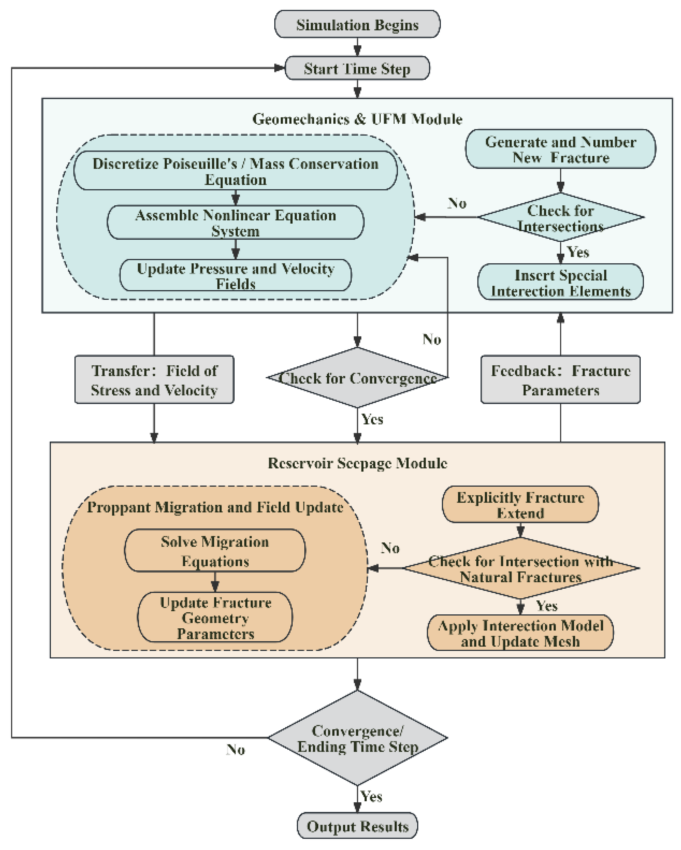
As shown in Figure 2, the coupled numerical solution is implemented within a rigorous time-stepping framework, which explicitly divides the computation into two interacting modules: the Geomechanics and UFM Module and the Reservoir Seepage Module. At each time step, the workflow initiates in the Geomechanics Module, where the in situ stress field is updated, and the fracture propagation criteria are evaluated. If propagation occurs, the fracture topology (length, width, and height) is updated along the direction of the local maximum principal stress. Crucially, the updated fracture geometry is converted into fracture conductivity, which serves as the key coupling parameter transferred to the Seepage Module. Subsequently, the Seepage Module updates the grid permeability and solves the nonlinear system of mass conservation equations to obtain the pressure and saturation distributions. The resulting pore pressure changes are then fed back to the Geomechanics Module to update the induced stress field (stress shadow effect), forming a bi-directional coupling loop. This iterative process continues until the simulation period concludes, ensuring that both dynamic fracture extension and multiphase flow behavior are accurately captured.

3. Reservoir Characterization and Sweet Spot Identification

3.1. Reservoir Characteristics and History Matching of Production Dynamics

This study employs the proposed model to simulate the ultra-low permeability field (CP) in the Ordos Basin. Geologic and production data are sourced directly from the target reservoir to ensure model reliability. The reservoir features a gentle monocline structure dipping westward, targeting the Triassic Yanchang Formation with an effective reservoir thickness of 19.7 m. Well logging results indicate an average porosity of 11.7% and an average permeability of 0.38 × 10⁻³ μm². The maximum horizontal principal stress (${\sigma }_H$) is between 40.88 and 42.25 MPa, and the minimum horizontal principal stress (${\sigma }_h$) is between 34.74 and 36.60 MPa. The vertical stress ($S_v$) falls within 53.17 to 55.63 MPa, indicating a reverse strike-slip faulting stress regime. According to the accuracy requirements of the simulation, the modeled area covers 9.66 km². The main reservoir interval is discretized with a grid size of 20 m × 20 m × 2.8 m, resulting in a total of 2,898,000 grid blocks (138 × 175 × 120). Detailed statistical parameters for the grid discretization are listed in

Table 1. Reservoir characteristics and numerical model parameters.

Formation	Parameters					Property
	Average Porosity, %	Average Permeability, 10−3 μm2	${\mathit{\sigma }}_{\mathit{H}}$, MPa	${\mathit{\sigma }}_{\mathit{h}}$, MPa	${\mathit{S}}_{\mathit{v}}$, MPa	Mesh Elements	Mesh Area, km2
Yanchang	11.7	0.38	40.88–42.25	34.74–36.60	53.17–55.63	2,898,000	9.66

. The model includes three horizontal production wells and eight vertical injection wells.

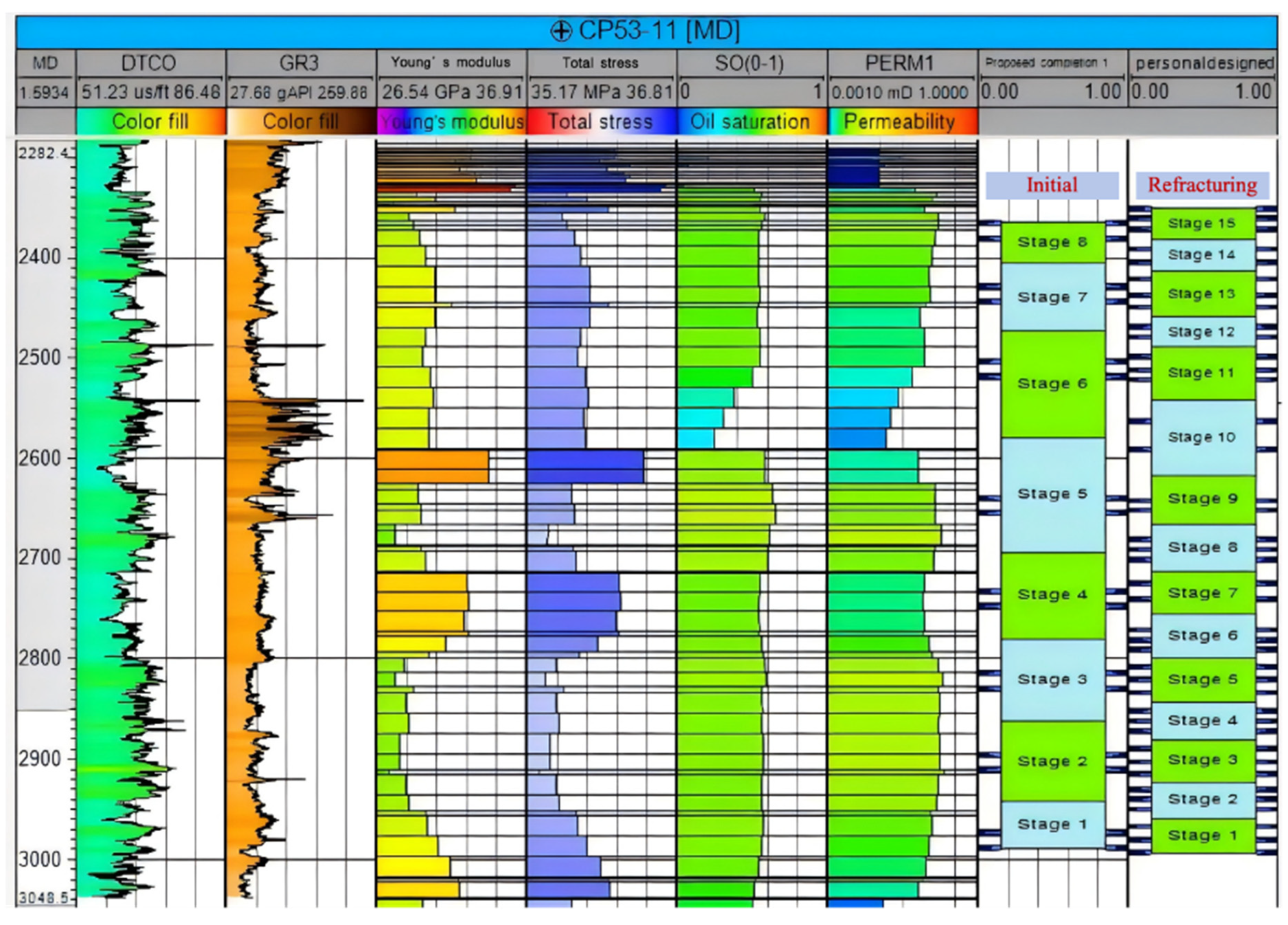
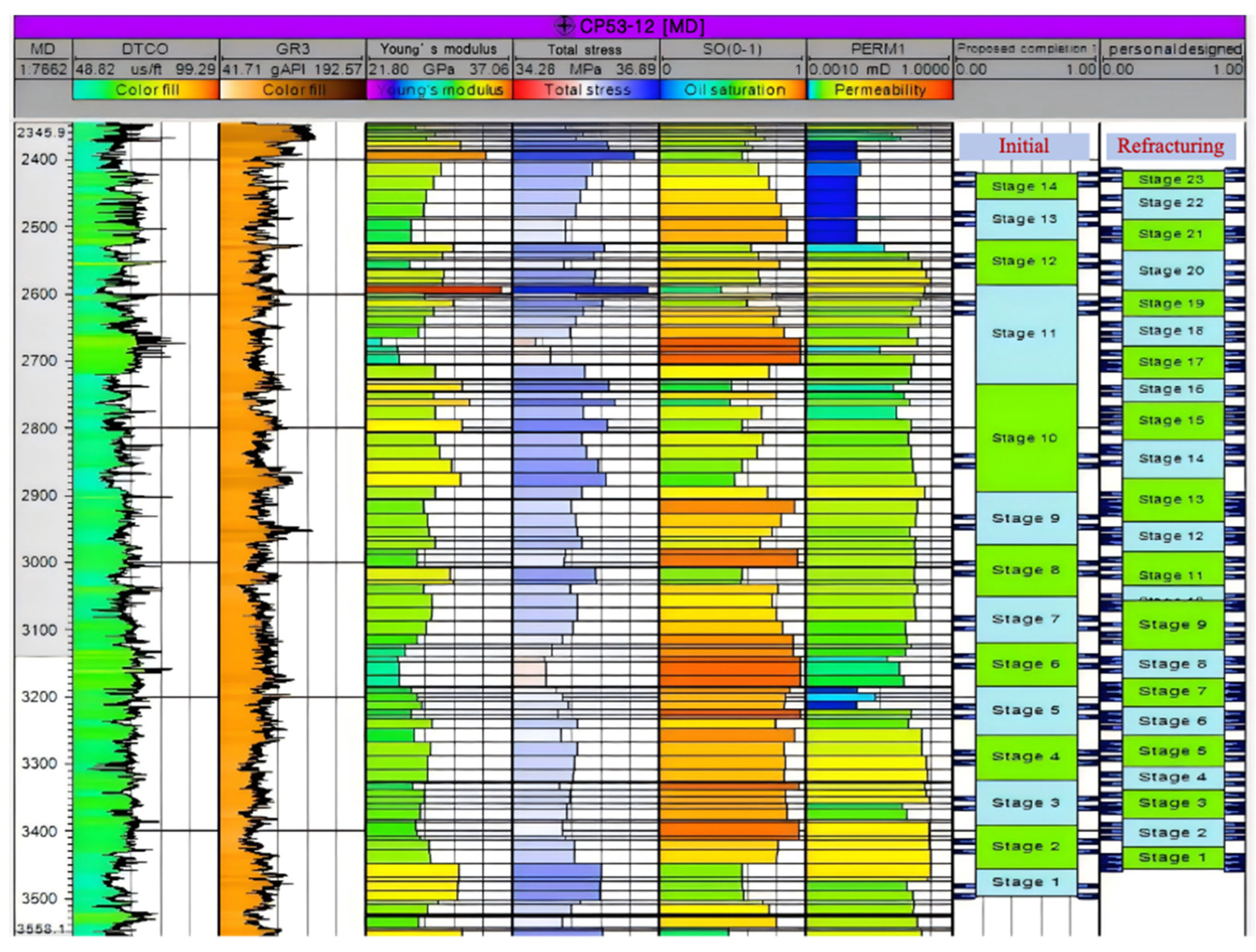
Based on geomechanical properties and fluid characteristics of target well groups CP53-11 and CP53-12, a high-resolution reservoir simulation model is constructed for production performance evaluation. Both wells are completed using hydraulic jet fracturing, with a measured depth of approximately 2295 m. For CP53-11, the horizontal section is 695 m in length, with 8 fracturing stages. The total injected fluid volume is 1933.5 m³, and the total proppant volume is 240 m³. For CP53-12, the horizontal section is 1096 m long with 14 stages, and the total fluid and proppant volumes are 2229.5 m³ and 415 m³, respectively. Detailed fracturing parameters are listed in

Table 2. Fracturing parameters for each well group.

NO.	Horizontal Section Length (m)	Stages	Clusters/Stage	Pumping Rate, m3	Proppant per Stage, m3	Injection Volume per Stage, m3
CP53-11	695	8	16	3.5	30.0	246.3
CP53-12	1096	14	28	3	29.6	159.5
Average	895.5	11	22	3.25	29.8	202.9

. Using the proposed model and incorporating the actual mechanical and physical properties of the reservoir, along with the designed fracturing schemes, simulations of fracture geometry and conductivity are conducted for both wells. The simulated fracture lengths for CP53-11 range from 143 to 244 m, with fracture conductivities between 0.46 and 1.18 D·m. For CP53-12, the fracture lengths range from 107 to 171 m, with conductivities between 0.47 and 0.82 D·m.

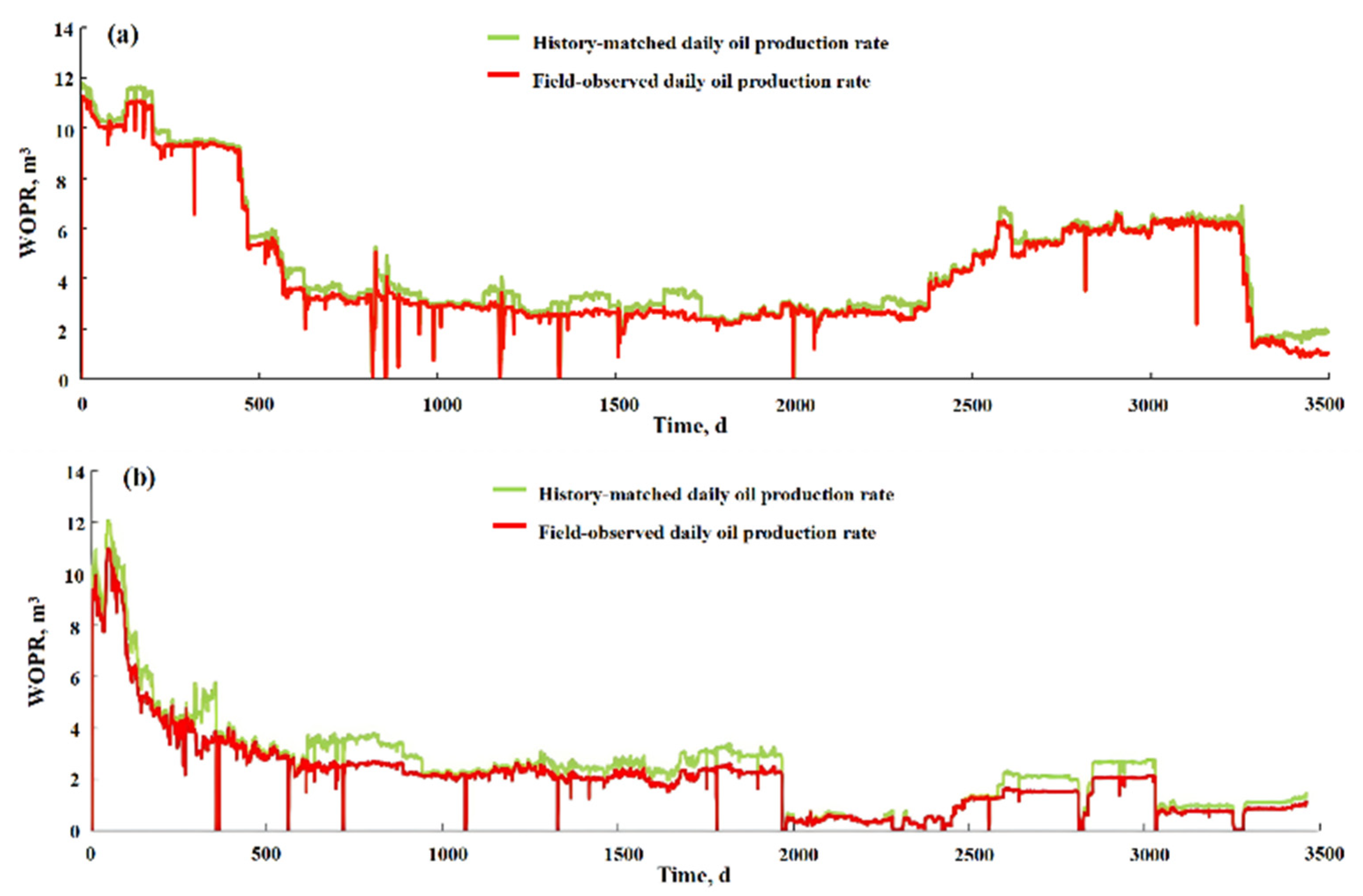
To ensure the fidelity of the numerical simulation, a rigorous history-matching process is conducted, using field production data from two representative horizontal wells, CP53-12 and CP53-11. The field production data, including daily oil rates and water cut, are measured using standard oilfield three-phase test separators installed at the wellhead, which are routinely calibrated and widely accepted for production monitoring in field operations. To address the limitation of single-parameter validation, the validation is conducted using a dual-parameter approach: matching the instantaneous “Daily Oil Production Rate” while simultaneously constraining the “Cumulative Oil Production” trend. Figure 3 presents the direct comparison between the numerical simulation results and the measured data under real exploitation conditions. As shown in Figure 3, the simulation curves exhibit a high degree of consistency with field records. Although minor discrepancies exist in the early flowback stage due to complex multiphase cleanup effects, the model effectively captures the characteristic rapid decline and the subsequent stable low-production behavior. Quantitative error analysis indicates that the relative error between the simulated and cumulative observed oil production is 4.2%. While a history-match error of 10–20% is generally acceptable in field-scale simulations, due to geological uncertainties [40], a threshold of within 5% is widely recognized as a high-precision standard in rigorous numerical studies to ensure the reliability of performance forecasting in complex ultra-low permeability reservoirs [41,42].

To verify the uniqueness of the history-matching solution, a sensitivity analysis is conducted on key uncertain parameters, including matrix permeability and fracture conductivity. Results indicated that cumulative production is most sensitive to matrix permeability deviations, with a ±10% change in permeability resulting in a ±15% variation in production, whereas fracture conductivity showed a lower sensitivity impact (<5%). The final matched parameters (Table 1) are selected within the geological constraints, to minimize the global error.

3.2. Characteristics of Energy Field Distribution

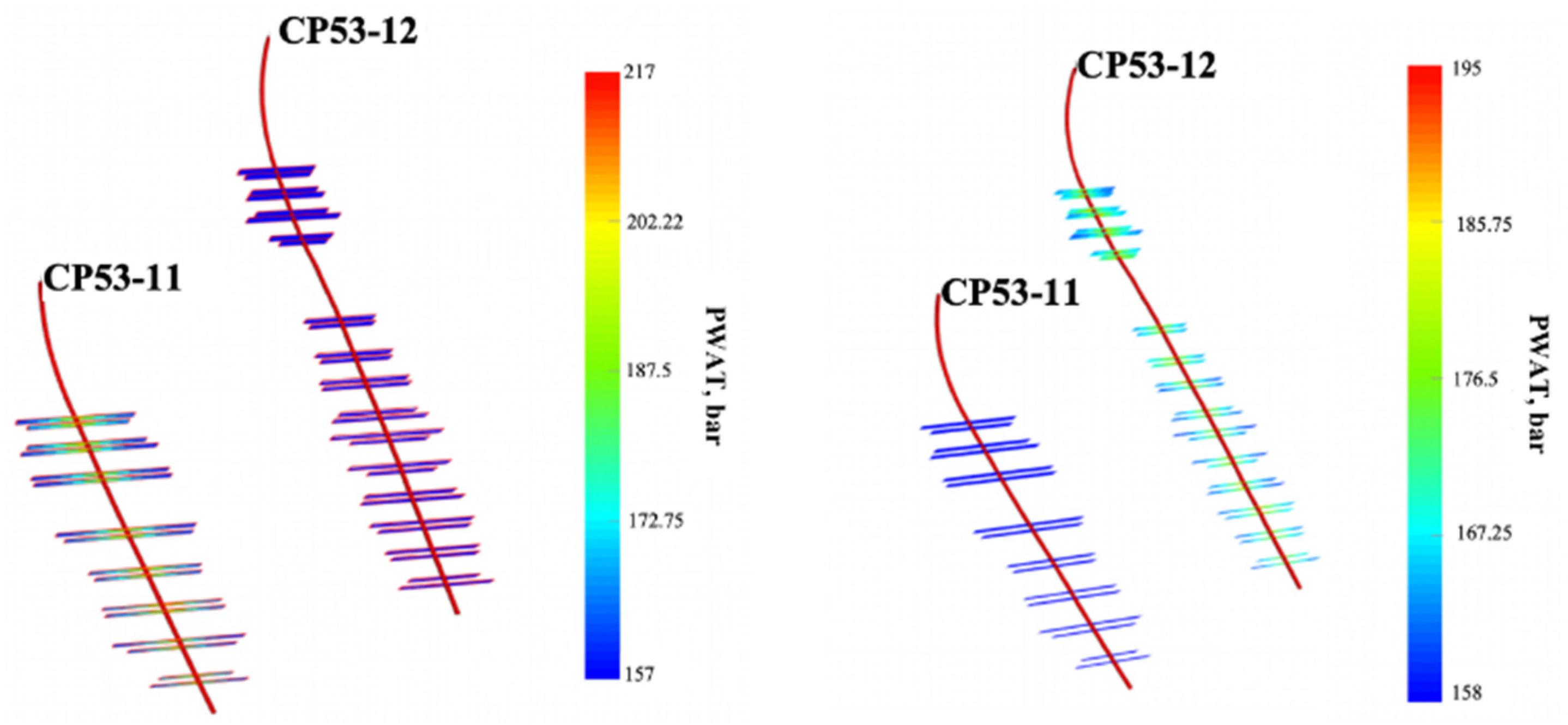
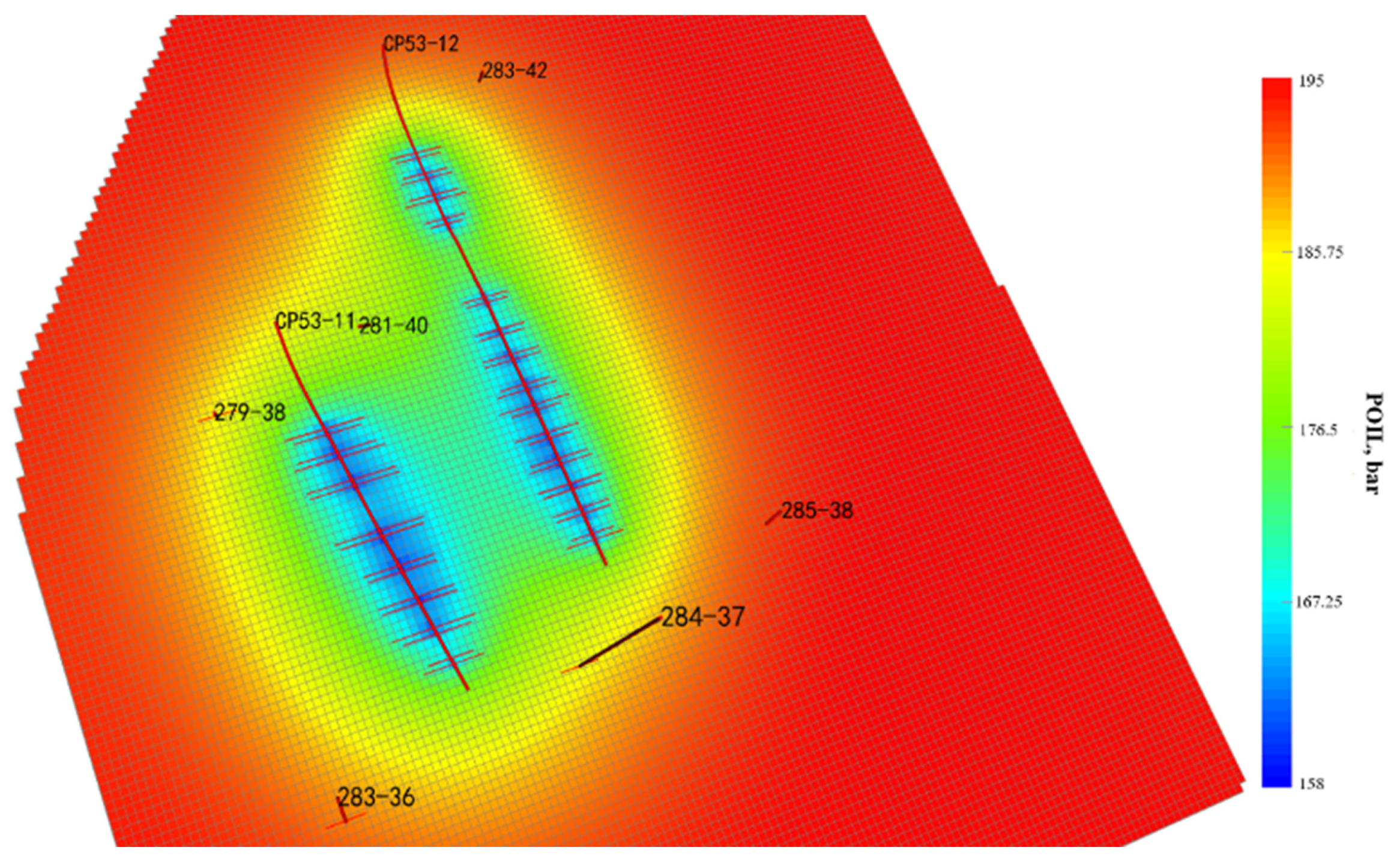
Field practices demonstrate that waterflooding patterns often have limited sweep efficiency in unconventional reservoirs. These approaches typically fail to adequately enhance pressure in remote zones, resulting in a common phenomenon of “strong near-well pressure support but weak far-field support”. Consequently, this leads to an imbalance in the early-stage injection profile and low sweep efficiency. Figure 4 shows the formation pressure response immediately after the initial hydraulic fracturing. It is evident that the initial hydraulic fracturing provides a certain degree of energy replenishment to the formation. For CP53-11 (8 stages, 16 clusters, 1933.5 m³ fluid), the pressure diffusion radius extends approximately 5 to 30 m from the wellbore, elevating the near-well pressure from 15.8 to 21.7 MPa. For CP53-12 (14 stages, 28 clusters, 2229 m³ fluid), a similar localized diffusion pattern (radius 5–25 m) is observed, increasing local pressure to 19.5 MPa. These simulation results quantitatively confirm the “strong near-well, weak far-field” energy distribution characteristic. The pressure wave fails to propagate effectively into the inter-well matrix, due to the uneven pressure distribution, leaving the vast areas between fracturing stages unstimulated.

Figure 5 further illustrates the reservoir pressure distribution after 10 years of depletion production. During this period, the average reservoir pressure declined significantly, from 20.8 MPa to 9.6 MPa. The blue zones in the map clearly identify the low-energy regions located between the two horizontal wells and in the inter-stage gaps. Efficient hydraulic communication between injection and production wells is not established, leading to severe energy depletion around the wellbores while leaving the far-field energy relatively isolated. This “stress-locking” effect creates substantial bypassed reserves (dead oil zones) that justify the necessity for the proposed refracturing strategy.

3.3. Characteristics of Residual Oil Saturation Field Distribution

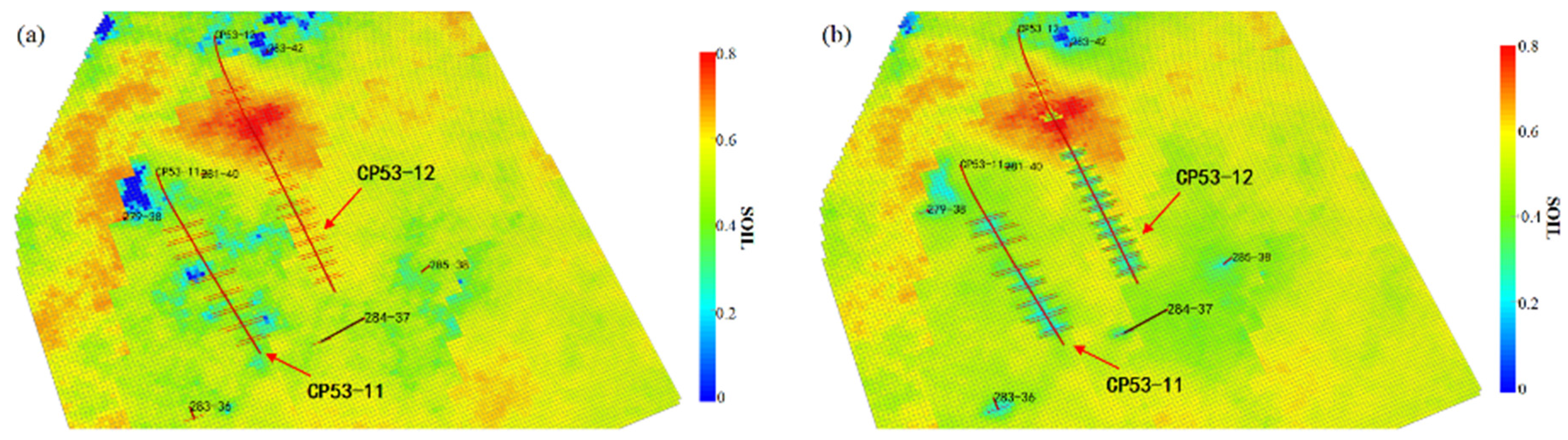
Residual oil saturation fields characterize the spatial distribution of drained and undrained oil phases in reservoirs during long-term waterflooding development. It serves as a scientific basis for evaluating development potential, accurately locating residual oil zones, optimizing development strategies, and ultimately maximizing recovery. The history-matched reservoir simulation model reveals the residual oil distribution patterns around producers and injectors. Comparative analysis of oil saturation before production and after waterflooding, with distinct “remaining oil rich zones”, are identified as shown in Figure 6. These regions are predominantly located in the inter-stage areas, distant from the primary fractures, with an effective drainage radius of only 5 to 30 m. Quantitative analysis indicates that post-fracturing residual oil saturation remains as high as 73.6% in Well CP53-12 and 59.6% in Well CP53-11 (indicated by the red/orange spectrum), with a saturation reduction of only 2%. This clear disparity in saturation distribution provides the geological basis for the subsequent infill fracturing design.

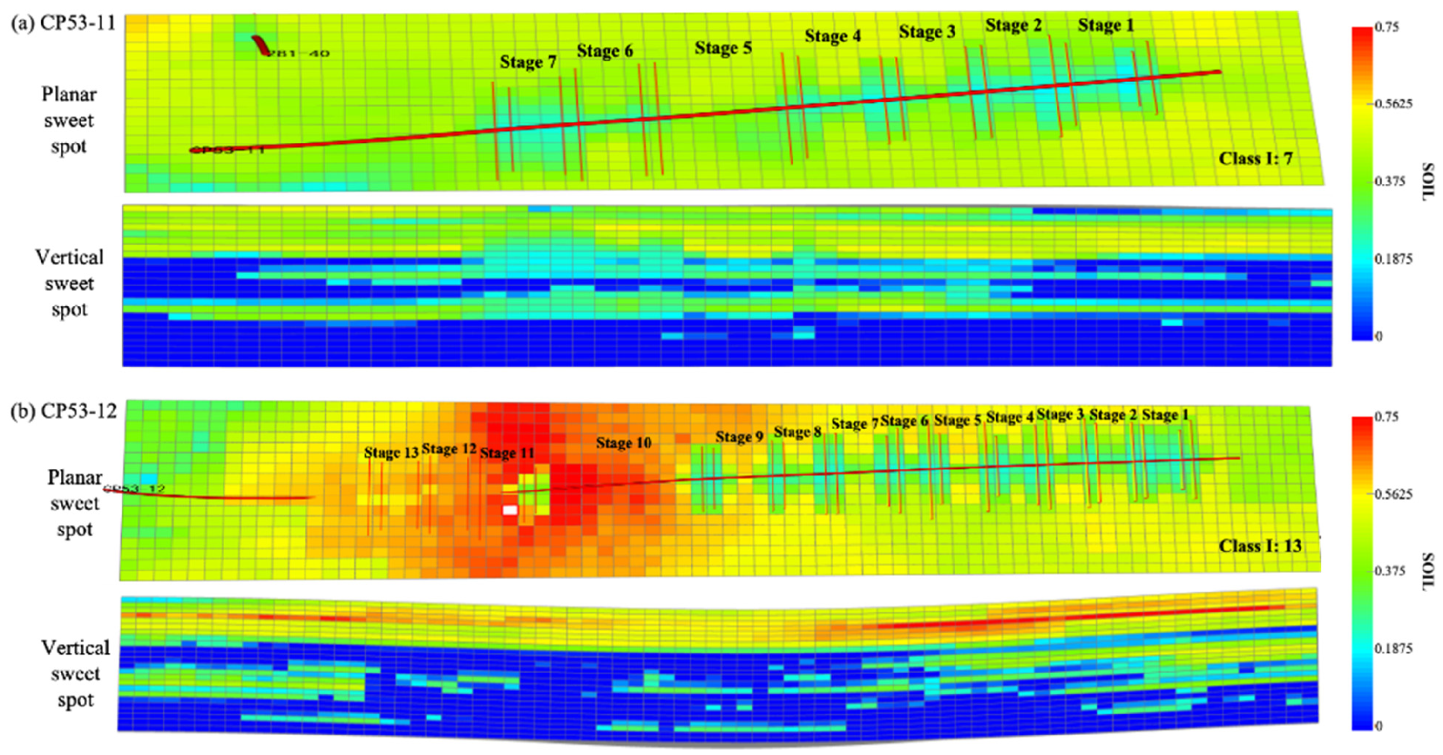
Figure 7 illustrates the distribution characteristics of inter-stage remaining oil. Simulation results indicate that a significant volume of residual oil between fracturing stages remains effectively unutilized. To characterize this potential, a zonation analysis is performed on the target area, based on the average oil saturation within the 3D inter-stage volume, integrating both planar and vertical sweet-spot characteristics along the horizontal wellbore. Statistical analysis of well logging data indicates that oil saturation in the study area primarily ranges from 10% to 78.5%, with a field-wide average of 24.9%. Notably, the average oil saturation in the primary productive layers (“sweet spots”) is 50.5%. Given the relatively homogeneous porosity and permeability distribution within the target matrix, residual oil saturation serves as the primary differentiator for production potential. Therefore, consequently, a remaining oil saturation classification standard, which is widely recognized in the tight oil development of the Ordos Basin, is adopted: Class I (So ≥ 0.50), Class II (0.25 ≤ So < 0.50), and Class III (0 < So < 0.25). This criterion aligns with local field practices, where Class I corresponds to the mobile oil saturation threshold in this ultra-low permeability matrix, representing the primary target for infill fracturing. Based on this evaluation, 7 and 13 Class I geological sweet spot segments are identified in well groups CP53-11 and CP53-12, respectively, delineating the precise target zones for the refracturing design.

4. Optimization of Refracturing Strategies and Parameters

Dynamic evaluation of energy field evolution and residual oil saturation distribution during fracturing development provides the foundation for this study. Centered on the core concept of “precision volumetric fracturing with integrated energy replenishment”, we propose a theoretical framework for refracturing key technologies and parameter optimization. (a) Replacing the traditional “refracturing of old fractures with regional energy supplementation” with optimized fracture spacing to generate a more complex fracture network and improve reservoir utilization. (b) Coupling the dynamic evolution of energy field and the seepage field, enhancing formation energy through combined water injection and fracturing to reconstruct the energy field and increase fracture complexity. (c) Multi-scale evaluation of the potential for residual oil recovery to guide the design of repeated fracturing parameters and improve well network deployment to achieve fracturing-energy replenishment coordinated development.

4.1. Optimization of Refracturing and Densified Fracture Strategy

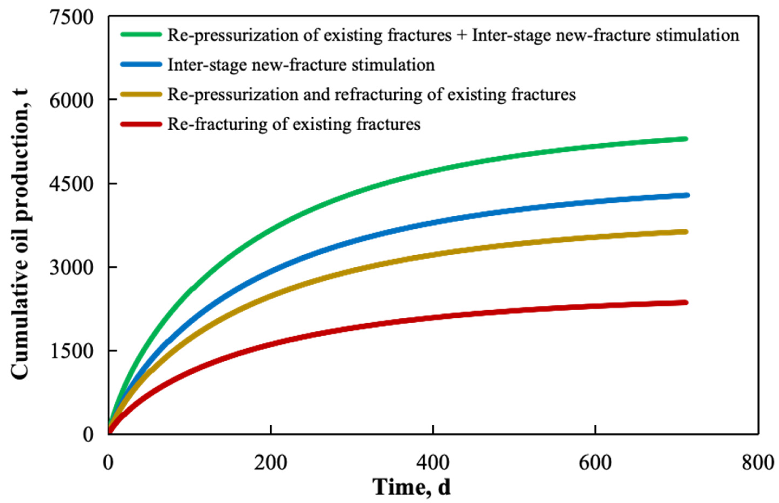
Previous analysis highlights significant undeveloped reserves in inter-well and inter-fracture zones, offering considerable potential for refracturing. Through detailed characterization of fracture networks and residual oil distribution, simulation studies (Figure 8) are conducted to maximize recovery from these fracture-controlled reserves. The results demonstrate the limited efficacy of conventional “re-pressurization and re-fracturing of existing fractures”. Instead, the optimized strategy—transitioning to “Re-pressurization of existing fractures + Inter-stage new fracture stimulation”—significantly enhances the stimulated volume. This approach is forecast to increase cumulative production by 55.86%, compared to the baseline. While this specific value represents a theoretical maximum derived from the optimized numerical model, the observed production enhancement trend is consistent with recent field pilot tests in the adjacent blocks of the Ordos Basin, confirming the strategy’s potential for field application.

Based on logging-derived petrophysical and mechanical parameters, a reservoir geological and engineering sweet-spot evaluation model is established. Simultaneously considering spacing between new and existing fractures and near-well residual oil distribution, refracturing is performed in inadequately stimulated zones, and additional fractures are placed between initial fracturing stages, to enhance reservoir stimulation. As shown in Figure 9, the number of refracturing stages in CP53-11 increased from 8 to 15, and from 14 to 23 in CP53-12, after fracture redesign.

4.2. Inter-Fracture Energy Supplementation to Reconstruct Energy Field

During long-term development, the original formation energy gradually depletes, resulting in reduced seepage-driving force. Consequently, residual oil is trapped in low-permeability zones or blind spots not previously stimulated by fracturing [43,44]. Refracturing provides physical fracture modification and flow rate optimization to break the “energy-depletion–stress-locking–residual-oil-trapping” cycle in late stages of production.

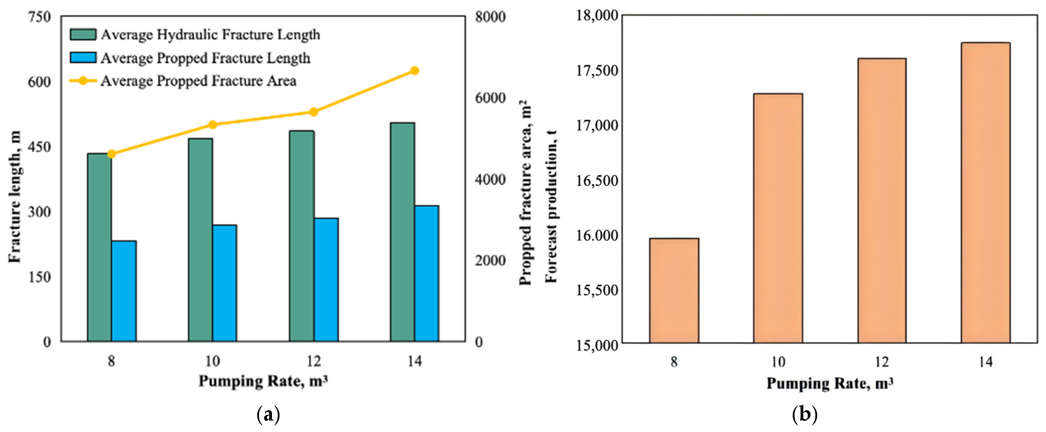
Based on the optimized refracturing-stage design, we evaluated the impact of different pumping rates (8, 10, 12, and 14 m³) on energy field evolution. These results served as initial conditions to estimate single-well performance using the standard of EUR performance. As shown in Figure 10a, production increases significantly with higher injection rates, accompanied by steady growth in hydraulic fracture length, propped fracture length, and propped area. However, the incremental production decreases from 24.28% to 10.78% when the pumping rate exceeds 12 m³/min. Fracture propagation analysis indicates that an optimal fracture half-length of 250 m is achieved at approximately 10 m³/min. Consequently, pumping rates between 10 and 12 m³/min are recommended, to yield the most favorable EUR performance (Figure 10b).

4.3. Energy Increase Optimization for Efficient Fracturing

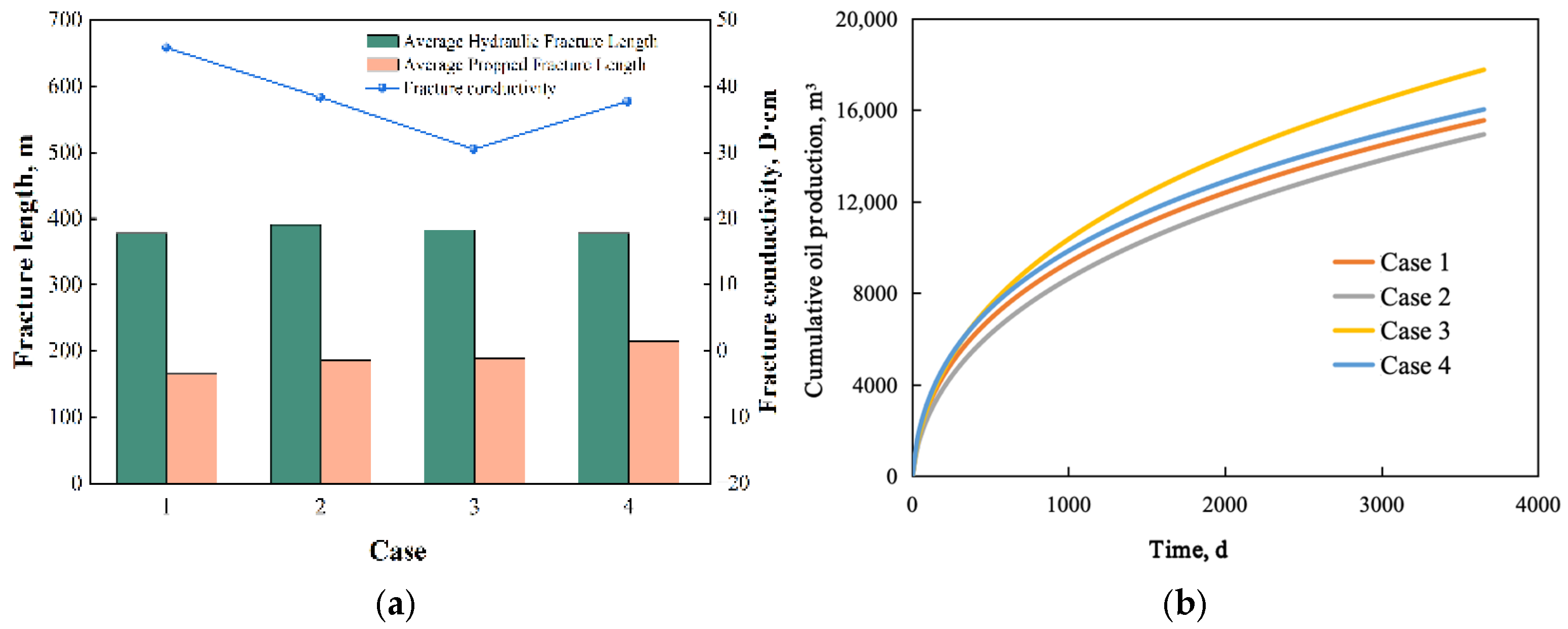
The core objective of reservoir energy increase lies in systematically optimizing fracturing parameters to generate complex multi-branch fracture networks, enhancing stimulated reservoir volume (SRV) and conductivity, thereby significantly improving residual oil recovery. To systematically investigate the impact of proppant size distribution on fracture conductivity and geometry, four simulation scenarios (Cases 1–4) are designed, based on varying mass ratios of coarse (20/40 mesh), medium (40/70 mesh), and fine (70/140 mesh) proppants. Specifically, Case 1 and Case 2 prioritize high conductivity using coarse-dominant ratios of 20/40 to 40/70 mesh at 4:1 and 2:1, respectively, without the addition of fine particles; Case 3 introduces a hybrid strategy with a ratio of 3:1:1 for 20/40, 40/70, and 70/140 mesh sizes, respectively, aiming to balance near-wellbore conductivity with far-field fracture access capability; whereas Case 4 shifts the focus toward medium-sized proppants with a 1:2 ratio of 20/40 to 40/70 mesh, to assess packing efficiency.

Simulation results (Figure 11a) indicate that Case 4 produced the longest propped-fracture length. However, the differences in average hydraulic- and propped-fracture lengths are relatively small, and the main difference lies in fracture conductivity. Case 4 achieves maximum propped length, though average hydraulic/propped lengths show minimal variation across schemes. Significant divergences emerge in fracture conductivity, with Case 1 exhibiting a peak conductivity that is 44.1–21.3 D·cm higher than Case 3. EUR simulations confirm Case 3’s superiority (Figure 11b), validating the small proportion of finer proppant (1:1:3 ratio) for maximizing ultimate recovery.

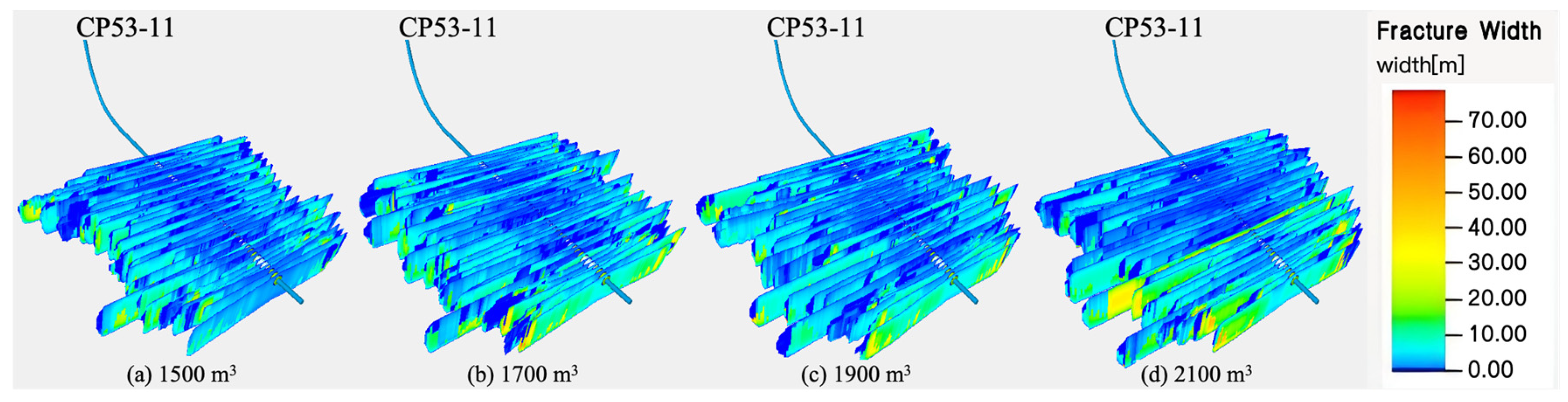
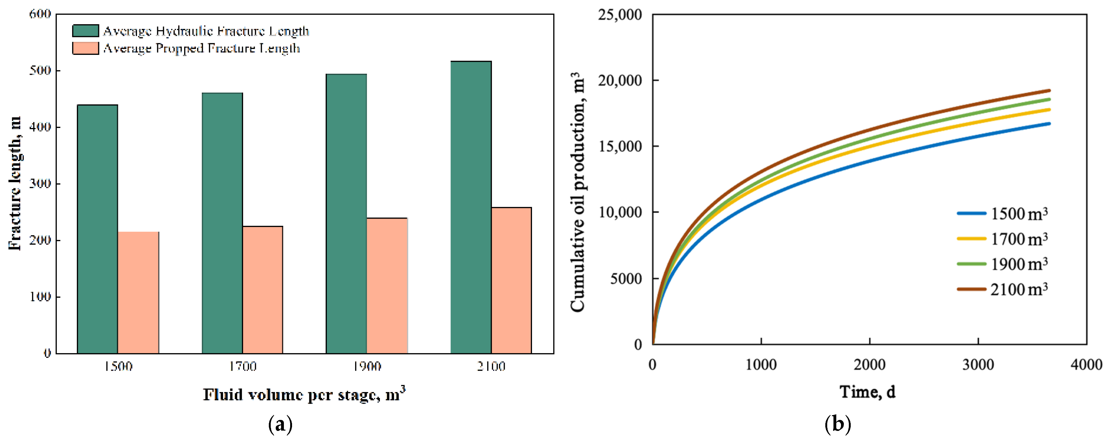
Treatment involving injected fluid-volume optimization proves equally critical during fracturing operations. A reasonable injection volume helps to reconstruct the in situ stress field, eliminate displacement blind zones, and enhance subsequent energy injection efficiency, by leveraging stress perturbations. To determine the optimal injected fluid volume per well, the design objective is set as the optimization of fracture half-length. Horizontal production Well CP53-11 is selected as a case study, to demonstrate the validity of the simulation results. The simulated fracture geometries under different scenarios are shown in Figure 12. As the injected fluid volume increased, both hydraulic and propped fracture lengths increased accordingly, though the change in propped fracture length is relatively minor—a result also confirmed by the fracture parameter comparison in Figure 13a. However, production forecast results showed that although oil production increased with fluid volume, the rate of increase diminished after 1700 m³, and the overall difference between scenarios became marginal, indicating the existence of an optimal value (Figure 13b). These results suggest that, in the studied area, controlling the single-stage fluid volume between 1700 and 1900 m³ yields the highest fluid-utilization efficiency.

4.4. Further Discussion

Comprehensive exploration of refracturing strategies is pivotal for the efficient development of unconventional reservoirs, representing a continuous industry evolution from primary depletion to advanced EOR techniques. Unlike the brittle shale plays in North America (e.g., Bakken and Eagle Ford), where refracturing focuses primarily on volume stimulation, the ultra-low permeability tight sandstone of the Ordos Basin exhibits significantly stronger stress sensitivity. Consequently, simple physical refracturing is often insufficient. This study addresses this specific geological challenge by proposing a synergistic strategy that integrates “re-pressurization of existing fractures” with “inter-stage infill fracturing”.

Existing research in similar geological settings indicates that while conventional refracturing (re-opening old fractures without energy supplementation) typically yields an EUR increment of only 15–20%, due to severe pressure depletion, and pure infill fracturing achieves approximately 30–35%, by contacting bypassed reserves [45], our synergistic strategy is projected to achieve a significantly higher EUR increase, of 55.86%. This performance gap—an additional ~20–25% gain over traditional methods—quantitatively confirms that re-pressurization is critical in preventing fracture closure in high-stress-sensitivity reservoirs, distinguishing this approach from purely volume-driven fracturing.

However, while the numerical model predicts substantial theoretical gains, field implementation faces inherent operational constraints that may temper these results. The primary concern is proppant embedment and long-term conductivity degradation. The current simulation assumes ideal proppant placement; yet, in reality, proppant embedment into softer, clay-rich layers could accelerate conductivity decline, potentially reducing the effective duration of the refracturing benefit. Future work should incorporate constitutive models for long-term creep and embedment, to further refine predictions. Furthermore, the operational risk of “frac hits”—where new fractures destructively interfere with existing ones—remains a concern. Although the spacing optimization proposed in this study serves to mitigate this risk, real-time microseismic monitoring is strongly recommended during field execution, to enable the dynamic adjustment of pumping parameters.

5. Conclusions

Based on the coupled geomechanics-matrix–fracture-seepage model and the numerical simulation of ultra-low permeability reservoirs in the Ordos Basin, the following conclusions are drawn:

• Initial hydraulic fracturing establishes limited effective displacement systems, with pressure diffusion radii ranging only from 5 to 30 m. The root cause of poor recovery is the “stress-locking” effect and the resulting “strong near-well, weak far-field” pressure distribution.
• The proposed strategy of “Re-pressurization of existing fractures + Inter-stage new fracture stimulation” synthesizes two mechanisms: it restores formation energy in depleted zones and reconstructs the formation energy field, leading to a theoretical production increase of 55.86%. This specific value corresponds to the theoretical maximum derived from the optimized numerical model, which is in agreement with the production enhancement trend observed during pilot tests in adjacent blocks.
• Precise parameter matching with geological sweet spots (Class I: So ≥ 0.50) is a prerequisite for success. Optimization indicates that for reservoirs with similar geological characteristics to the Ordos Basin, a moderate pumping rate (10–12 m³/min) combined with optimized fluid intensity (1700–1900 m³/stage) achieves the best balance between fracture complexity and containment, preventing inefficient height growth while maximizing reservoir contact.
• While increasing fluid volume enhances fracture length, an inflection point exists beyond which production gains diminish. Furthermore, optimizing the proppant schedule to include a specific ratio of smaller mesh sizes (e.g., 20/40, 40/70, and 70/140 combinations) balances fracture conductivity with propped length, maximizing the comprehensive sweep efficiency.

References

1. Jia, C. Breakthrough and Significance of Unconventional Oil and Gas to Classical Petroleum Geology Theory. Pet. Explor. Dev. 2017, 44, 1–10. [Google Scholar] [CrossRef]
2. Liu, X.; Li, S.; Zhou, X.; Chen, X.; Liu, J.; Guo, Q.; Wei, J.; Liao, Y. New Fields, New Types and Resource Potentials of Petroleum Exploration in Ordos Basin. Acta Pet. Sin. 2023, 44, 2070–2090. [Google Scholar] [CrossRef]
3. Hu, S.; Tao, S.; Wang, M.; Pang, Z.; Bai, B.; Chen, Y.; Lu, S.; Chen, Y.; Yang, Y.; Jin, X.; et al. Migration and Accumulation Mechanisms and Main Controlling Factors of Tight Oil Enrichment in a Continental Lake Basin. Pet. Explor. Dev. 2023, 50, 547–557. [Google Scholar] [CrossRef]
4. Jia, C.; Zou, C.; Yang, Z.; Zhu, R.; Chen, Z.; Zhang, B.; Jiang, L. Significant Progress of Continental Petroleum Geological Theory in Basins of Central and Western China. Pet. Explor. Dev. 2018, 45, 573–588. [Google Scholar] [CrossRef]
5. Song, Y.; Luo, Q.; Jiang, Z.; Yang, W.; Liu, D. Enrichment of Tight Oil and Its Controlling Factors in Central and Western China. Pet. Explor. Dev. 2021, 48, 492–506. [Google Scholar] [CrossRef]
6. Yang, H.; Liu, X.; Huang, D.; Lan, Y.; Wang, S. Natural Gas Exploration and Development in Changqing Oilfield and Its Prospect in the 13th Five-Year Plan. Nat. Gas Ind. B 2016, 3, 291–304. [Google Scholar] [CrossRef]
7. Barree, R.D.; Miskimins, J.L.; Svatek, K.J. Reservoir and Completion Considerations for the Refracturing of Horizontal Wells. SPE Prod. Oper. 2017, 33, 1–11. [Google Scholar] [CrossRef]
8. Cao, Y.; Feng, B.; Cui, Z.; Duan, X.; Zhao, J. Numerical Simulation Study of Segmented Hydraulic Fracturing in Horizontal Wells of Fractured Hot Dry Rocks, at the U.S. FORGE Site. Geoenergy Sci. Eng. 2025, 249, 213790. [Google Scholar] [CrossRef]
9. Denney, D. Ranking Production Potential from Key Geological Drivers—Bakken Case Study. J. Pet. Technol. 2011, 63, 63–65. [Google Scholar] [CrossRef]
10. Han, B.; Cui, G.; Wang, Y.; Zhang, J.; Zhai, Z.; Shi, Y.; Yan, F.; Li, W. Effect of Fracture Network on Water Injection Huff-Puff for Volume Stimulation Horizontal Wells in Tight Oil Reservoir: Field Test and Numerical Simulation Study. J. Pet. Sci. Eng. 2021, 207, 109106. [Google Scholar] [CrossRef]
11. Male, F.; Duncan, I.J. The Paradox of Increasing Initial Oil Production but Faster Decline Rates in Fracking the Bakken Shale: Implications for Long Term Productivity of Tight Oil Plays. J. Pet. Sci. Eng. 2022, 208, 109406. [Google Scholar] [CrossRef]
12. Themig, D. New Technologies Enhance Efficiency of Horizontal, Multistage Fracturing. J. Pet. Technol. 2011, 63, 26–31. [Google Scholar] [CrossRef]
13. Guo, J.; Tao, L.; Zeng, F. Optimization of Refracturing Timing for Horizontal Wells in Tight Oil Reservoirs: A Case Study of Cretaceous Qingshankou Formation, Songliao Basin, NE China. Pet. Explor. Dev. 2019, 46, 153–162. [Google Scholar] [CrossRef]
14. Ma, X.; Hao, R.; Lai, X.; Zhang, Y.; Ma, Z.; He, M.; Xiao, Y.; Bi, M.; Ma, X. Field Test of Volume Fracturing for Horizontal Wells in Sulige Tight Sandstone Gas Reservoirs, NW China. Pet. Explor. Dev. 2014, 41, 810–816. [Google Scholar] [CrossRef]
15. Guo, T. Key Geological Issues and Main Controls on Accumulation and Enrichment of Chinese Shale Gas. Pet. Explor. Dev. 2016, 43, 349–359. [Google Scholar] [CrossRef]
16. Zhang, Y.-J.; Li, Z.-W.; Guo, L.-L.; Gao, P.; Jin, X.-P.; Xu, T.-F. Electricity Generation from Enhanced Geothermal Systems by Oilfield Produced Water Circulating through Reservoir Stimulated by Staged Fracturing Technology for Horizontal Wells: A Case Study in Xujiaweizi Area in Daqing Oilfield, China. Energy 2014, 78, 788–805. [Google Scholar] [CrossRef]
17. Wei, J.; Huang, S.; Hao, G.; Li, J.; Zhou, X.; Gong, T. A Multi-Perforation Staged Fracturing Experimental Study on Hydraulic Fracture Initiation and Propagation. Energy Explor. Exploit. 2020, 38, 2466–2484. [Google Scholar] [CrossRef]
18. Zhang, G.Q.; Chen, M. Dynamic Fracture Propagation in Hydraulic Re-Fracturing. J. Pet. Sci. Eng. 2010, 70, 266–272. [Google Scholar] [CrossRef]
19. Tao, J.; Meng, S.; Cao, G.; Gao, Y.; Liu, H. Experimental Study on the Impact of Supercritical CO2 Soak Pre-Treatment on Re-Fracturing of Shale Oil Reservoirs. In Proceedings of the SPE Asia Pacific Oil & Gas Conference and Exhibition, Virtual, 12–15 November 2020; OnePetro: Richardson, TX, USA, 2020. [Google Scholar]
20. Liu, Z.; Li, X.; Wang, J.; Liu, R.; Wang, T.; Wang, Y.; Yan, Z.; Li, X. Study on Method of Sweet Spot Interval Identification of Tight Gas Reservoir in Horizontal Well. China Pet. Explor. 2021, 26, 117–125. [Google Scholar] [CrossRef]
21. Nolte, K.G. Fracturing-Pressure Analysis for Nonideal Behavior. J. Pet. Technol. 1991, 43, 210–218. [Google Scholar] [CrossRef]
22. Weng, X.; Kresse, O.; Cohen, C.; Wu, R.; Gu, H. Modeling of Hydraulic-Fracture-Network Propagation in a Naturally Fractured Formation. SPE Prod. Oper. 2011, 26, 368–380. [Google Scholar] [CrossRef]
23. Kresse, O.; Weng, X.; Gu, H.; Wu, R. Numerical Modeling of Hydraulic Fractures Interaction in Complex Naturally Fractured Formations. Rock Mech. Rock Eng. 2013, 46, 555–568. [Google Scholar] [CrossRef]
24. Taleghani, A.D.; Olson, J.E. How Natural Fractures Could Affect Hydraulic-Fracture Geometry. SPE J. 2013, 19, 161–171. [Google Scholar] [CrossRef]
25. Bhide, R.J.; Zhao, N.; McLennan, J.D.; Deo, M.D. Modeling Hydraulic Fracture Propagation in Low Permeability Reservoirs. In Proceedings of the 46th U.S. Rock Mechanics/Geomechanics Symposium, Chicago, IL, 24–27 June 2012; OnePetro: Richardson, TX, USA, 2012. [Google Scholar]
26. Li, J.; Zhu, Z.; Hua, W.; Wu, D.; Zhang, N.; Dong, S.; Guo, T. Numerical Simulation of Fracture Propagation during Temporary Plugging Staged Fracturing in Tight-Oil Horizontal Wells. ACS Omega 2024, 9, 18542–18555. [Google Scholar] [CrossRef] [PubMed]
27. Wang, Z.; Guo, J.; Qiao, L.; Liu, J.; Li, W. Matrix–Fracture Flow Transfer in Fractured Porous Media: Experiments and Simulations. Rock Mech. Rock Eng. 2022, 55, 2407–2423. [Google Scholar] [CrossRef]
28. Yu, J.; Li, N.; Hui, B.; Zhao, W.; Li, Y.; Kang, J.; Hu, P.; Chen, Y. Experimental Simulation of Fracture Propagation and Extension in Hydraulic Fracturing: A State-of-the-Art Review. Fuel 2024, 363, 131021. [Google Scholar] [CrossRef]
29. Wang, Q.; Wang, Y.; Wang, R.; Zhao, J.; Hu, Y.; Zhao, J. Evolution Law of Stress Induced by Pressure Depletion in Fractured Shale Reservoirs: Implications for Subsequent Refracturing and Infill Well Development. Petroleum 2025, 11, 71–83. [Google Scholar] [CrossRef]
30. Kresse, O.; Weng, X. Numerical Modeling of 3D Hydraulic Fractures Interaction in Complex Naturally Fractured Formations. Rock Mech. Rock Eng. 2018, 51, 3863–3881. [Google Scholar] [CrossRef]
31. Gu, H.; Weng, X.; Lund, J.; Mack, M.; Ganguly, U.; Suarez-Rivera, R. Hydraulic Fracture Crossing Natural Fracture at Non-Orthogonal Angles, A Criterion, Its Validation and Applications. SPE Prod. Oper. 2012, 27, 20–26. [Google Scholar]
32. Yong, R.; Zhou, F.-J.; Li, M.-H.; Song, Y.; Zhou, X.-J.; Zhao, Z.-H.; Li, B.; Qin, S.-Y. Effects of Fracturing Parameters on Fracture Unevenness During Large-Stage Multi-Cluster Fracturing in Horizontal Wells. Front. Energy Res. 2021, 9, 612486. [Google Scholar] [CrossRef]
33. Kanninen, M.F.; Popelar, C.A.; Saunders, H. Advanced Fracture Mechanics. J. Vib. Acoust. Stress Reliab. Des. 1988, 110, 419–420. [Google Scholar] [CrossRef]
34. Wu, K.; Olson, J.E. Simultaneous Multifracture Treatments: Fully Coupled Fluid Flow and Fracture Mechanics for Horizontal Wells. SPE J. 2014, 20, 337–346. [Google Scholar] [CrossRef]
35. Clark, P.E.; Quadir, J.A. Prop Transport in Hydraulic Fractures: A Critical Review of Particle Settling Velocity Equations. In Proceedings of the SPE/DOE Low Permeability Gas Reservoirs Symposium, Denver, CO, USA, 27–29 May 1981; OnePetro: Richardson, TX, USA, 1981. [Google Scholar]
36. Adachi, J.; Siebrits, E.; Peirce, A.; Desroches, J. Computer Simulation of Hydraulic Fractures. Int. J. Rock Mech. Min. Sci. 2007, 44, 739–757. [Google Scholar] [CrossRef]
37. Daneshy, A.A. Numerical Solution of Sand Transport in Hydraulic Fracturing. J. Pet. Technol. 1978, 30, 132–140. [Google Scholar] [CrossRef]
38. Warpinski, N.R.; Teufel, L.W. Influence of Geologic Discontinuities on Hydraulic Fracture Propagation (Includes Associated Papers 17011 and 17074). J. Pet. Technol. 1987, 39, 209–220. [Google Scholar] [CrossRef]
39. Geertsma, J.; De Klerk, F. A Rapid Method of Predicting Width and Extent of Hydraulically Induced Fractures. J. Pet. Technol. 1969, 21, 1571–1581. [Google Scholar] [CrossRef]
40. Baker, R.O.; Chugh, S.; Mcburney, C.; McKishnie, R. History Matching Standards; Quality Control and Risk Analysis for Simulation. In Proceedings of the Canadian International Petroleum Conference, Calgary, AB, Canadian, 13–15 June 2006; OnePetro: Richardson, TX, USA, 2006. [Google Scholar]
41. Pal, N.; Mandal, A. Compositional Simulation Model and History-Matching Analysis of Surfactant-Polymer-Nanoparticle (SPN) Nanoemulsion Assisted Enhanced Oil Recovery. J. Taiwan Inst. Chem. Eng. 2021, 122, 1–13. [Google Scholar] [CrossRef]
42. Yu, Y.; Liu, S.; Liu, Y.; Bao, Y.; Zhang, L.; Dong, Y. Data-Driven Proxy Model for Forecasting of Cumulative Oil Production during the Steam-Assisted Gravity Drainage Process. ACS Omega 2021, 6, 11497–11509. [Google Scholar] [CrossRef]
43. Craig, D.P.; Barree, R.D.; Warpinski, N.R.; Blasingame, T.A. Fracture Closure Stress: Reexamining Field and Laboratory Experiments of Fracture Closure Using Modern Interpretation Methodologies. In Proceedings of the SPE Annual Technical Conference and Exhibition, San Antonio, TX, USA, 9 October 2017; SPE: San Antonio, TX, USA, 2017. [Google Scholar]
44. Urban, E.; Orozco, D.; Fragoso, A.; Selvan, K.; Aguilera, R. Refracturing Vs. Infill Drilling—A Cost Effective Approach to Enhancing Recovery in Shale Reservoirs. In Proceedings of the SPE/AAPG/SEG Unconventional Resources Technology Conference, San Antonio, Texas, USA, 1 August 2016; OnePetro: Richardson, TX, USA, 2016. [Google Scholar]
45. Zhang, X.; Ren, J.; Feng, Q.; Wang, X.; Wang, W. Prediction of Refracturing Timing of Horizontal Wells in Tight Oil Reservoirs Based on an Integrated Learning Algorithm. Energies 2021, 14, 6524. [Google Scholar] [CrossRef]
Figure 1. Connectivity pattern of the unstructured DFN model. (The background grid represents the matrix domain. Matrix grids are shown as gray background. Natural fracture surfaces are in brown, while hydraulic fractures are in blue. σ H and σ h denote the maximum and minimum horizontal principal stresses, respectively).
Energies 19 01022 g001
Figure 2. Flowchart of the coupled simulation algorithm.
Energies 19 01022 g002
Figure 3. History matching results of daily oil production rate for Wells (a) CP53-11 and (b) CP53-12.
Energies 19 01022 g003
Figure 4. Effect of different fracturing treatment size on pressure transmission response for Wells CP53-11 and CP53-12.
Energies 19 01022 g004
Figure 5. Formation pressure distribution for Wells CP53-11 and CP53-12 after 10 years.
Energies 19 01022 g005
Figure 6. Comparison of oil saturation distribution for well groups CP53-11 and CP53-12: (a) initial state before production, and (b) residual oil distribution after long-term waterflooding.
Energies 19 01022 g006
Figure 7. Planar and vertical distribution of residual oil saturation for CP53-11 and CP53-12.
Energies 19 01022 g007
Figure 8. Cumulative oil production under different development strategies.
Energies 19 01022 g008
Figure 9. Optimized refracturing stage design for Wells CP53-11 and CP53-12.
Energies 19 01022 g009aEnergies 19 01022 g009b
Figure 10. Fracture parameters and production forecast of a single well under different pumping rates. (a) Fracture-propagation simulation parameters; (b) post-fracturing numerical production forecast of EUR.
Energies 19 01022 g010
Figure 11. Fracture parameters and production forecast of a single well under different proppant cases. (a) Fracture-propagation simulation parameters; (b) post-fracturing numerical production forecast of EUR.
Energies 19 01022 g011
Figure 12. Fracture geometry of Well CP53-11 under different refracturing cases.
Energies 19 01022 g012
Figure 13. Fracture parameters and production forecast of a single well under different injected fluid volume. (a) Fracture-propagation simulation parameters; (b) post-fracturing numerical production forecast of EUR.
Energies 19 01022 g013