


Abstract
The photovoltaic field has seen significant development in recent years, with continuously expanding installation capacity and increasing grid integration. However, due to the intermittency of solar energy and meteorological variability, PV output power poses serious challenges to grid security and dispatch reliability. Traditional forecasting methods largely rely on modeling historical power and meteorological data, often neglecting the consideration of cloud movement, which constrains further improvement in prediction accuracy. To enhance prediction accuracy and model interpretability, this paper proposes a dual-branch attention-based PV power prediction model that integrates physical features from ground-based cloud images. Regarding input features, a cloud segmentation model is constructed based on the vision foundation model DINO encoder and an improved U-Net decoder to obtain cloud cover information. Based on deep feature point detection and an attention matching mechanism, cloud motion vectors are calculated to extract cloud motion speed and direction features. For feature processing, feature attention and temporal attention mechanisms are introduced, enabling the model to learn key meteorological factors and critical historical time steps. Structurally, a parallel architecture consisting of a linear branch and a nonlinear branch is adopted. A context-aware fusion module adaptively combines the prediction results from both branches, achieving collaborative modeling of linear trends and nonlinear fluctuations. Comparative experiments were conducted using two years of engineering data. Experimental results demonstrate that the proposed model outperforms the benchmarks across multiple metrics, validating the predictive advantages of the dual-branch structure that integrates physical features under complex weather conditions.
1. Introduction
Rising carbon emissions and fossil fuel dependence necessitate clean energy development. Solar PV has expanded rapidly but exhibits highly variable and stochastic output due to irradiation, weather, and cloud dynamics, challenging grid stability and dispatch reliability. Therefore, achieving high-precision photovoltaic power prediction has become a key core technology for ensuring grid integration capacity, optimizing power plant operation management, and enhancing the economic performance of PV power generation [1,2].
In recent years, photovoltaic power prediction technology has seen significant development. From the perspective of model evolution, PV power prediction models have transitioned from physical models and statistical models to machine learning and deep learning models. Physical models are based on weather data and component parameters of PV power plants, constructing mapping relationships from meteorological parameters such as solar radiation to output power [3]. Scholars have predicted PV output by modeling the mathematical relationships between internal physical processes of PV components (e.g., photoelectric conversion, carrier transport) and external meteorological conditions (irradiance, temperature) [3]. This modeling process is complex, requires high data quality, and often performs poorly under complex weather conditions. Statistical models mostly employ techniques such as ARIMA (Autoregressive Integrated Moving Average) and exponential smoothing. By establishing relationships between past and future power outputs and making explicit parametric assumptions about the data generation process based on mathematical formulas and probability theory [4,5], these methods struggle to describe complex nonlinear characteristics and handle various complex weather conditions, as the nature of PV output power is far more intricate.
The development of machine learning methods such as Random Forest and Support Vector Regression has led to a significant improvement in the accuracy of photovoltaic power prediction [6,7]. Through standardized benchmarking, extensive experimentation, and scientific comparison, scholars have applied 24 machine learning models (e.g., Kernel Ridge Regression, Multi-Layer Perceptron, Decision Tree) to PV power prediction based on Numerical Weather Prediction (NWP), achieving favorable results [8].
With the development of deep learning, a large number of excellent time-series models have been applied to the field of power forecasting. Among the most classic are Recurrent Neural Networks (RNNs) and Long Short-Term Memory (LSTM) networks. Leveraging their powerful ability to capture temporal features, these models have elevated the accuracy of photovoltaic power prediction to new heights [9,10,11,12]. Scholars have combined Genetic Algorithm (GA) with the AMODE (Adaptive Multi-Objective Differential Evolution) algorithm to optimize Bi-directional LSTM (BiLSTM) networks. The optimized models significantly outperform traditional models in terms of accuracy metrics, stability, and generalization ability [13]. RNN-based models are limited by issues like vanishing gradients and difficulty in modeling long sequences, while Convolutional Neural Networks (CNNs) cannot capture dynamic temporal dependencies. In recent years, with the progress in artificial intelligence, Transformer-based models have garnered attention from scholars, further advancing the development of temporal and multimodal prediction. Their core self-attention mechanism can capture long-sequence dependencies and offers high parallelism [14,15,16]. Scholars have proposed integrated frameworks combining physical modeling, multivariate meteorological data, and Transformer neural networks, capable of achieving high-precision and strongly generalizable PV power prediction [15]. Comparative experiments have demonstrated that a combined Transformer–LSTM model outperforms individual CNN, Gated Recurrent Unit (GRU), LSTM, or Transformer models in terms of both accuracy and stability [15]. Subsequently, improved architectures such as Informer and Autoformer have significantly enhanced the efficiency and stability of Transformer in time series forecasting tasks, establishing Transformer as a new trend in time series prediction models [17,18]. Scholars proposed a BiLSTM–Informer hybrid model, incorporating innovative feature optimization methods and real-time network inference validation, which substantially improved the accuracy of both short-term and long-term predictions [18]. Another study presented an improved Autoformer model for short-term PV power prediction, integrating a multi-scale framework and a de-stationary attention mechanism, and validated its superior performance over other baseline models on datasets with different temporal resolutions [17].
Meanwhile, to enhance model capacity and robustness, hybrid or ensemble architectures have become another significant trend in the development of forecasting models. The modeling approach has gradually shifted from single models to hybrid and ensemble models. Researchers combine models with different strengths through cascading (e.g., GRU-CNN [19]), stacking (e.g., Stacking ensembles [20]), or voting methods [21] to optimize prediction outcomes. Scholars constructed a GRU-CNN deep learning network, utilizing weather forecast data and historical power data to achieve weekly PV power forecasting, which outperformed multiple baseline models [19]. Scholars proposed a novel two-layer stacked ensemble model, Stack-ETR, where the fusion strategy significantly improved the accuracy of PV power generation forecasting [20]. Scholars introduced an ensemble voting model for solar irradiance forecasting, demonstrating that the weighted average voting model outperformed all individual algorithms in most cases [21]. These practical results indicate that hybrid models offer more stable advantages compared to single models. However, existing hybrid methods primarily focus on model combination techniques in their structure and employ static or fixed fusion strategies (e.g., weighted averaging) for result integration. They are unable to dynamically adjust the contributions of sub-models based on real-time weather contexts, making it challenging to accurately address the dynamic evolution of linear trend components (e.g., diurnal cycles) and nonlinear disturbance components (e.g., sudden cloud occlusion) in PV power, which vary with conditions. From a modeling perspective, such methods represent more of an engineering-level model ensemble rather than a structural modeling approach based on signal generation mechanisms.
In terms of input sources, the input data for PV forecasting have also evolved from single to multimodal. Early studies primarily relied on historical power data and meteorological observations such as irradiance, temperature, and humidity. With advancements in weather forecasting and computer vision technologies, an increasing number of studies have begun to incorporate external information such as Numerical Weather Prediction (NWP) [22], satellite cloud imagery [23,24], and ground-based cloud imagery [25,26,27] to enrich model inputs and improve forecasting accuracy. Ground-based cloud imagery, due to its high acquisition frequency and resolution, as well as its ability to directly reflect cloud movement around PV power plants, has gradually become an important data source for short-term PV forecasting. Scholars proposed a hybrid Swin Transformer-CNN-LSTM framework based on ground-based image sequences and historical PV power data to capture global spatial features of cloud movement in images for short-term power forecasting [28]. Scholars employed CNNs to process static images while integrating the latest power measurements and used CNN-LSTM to process dynamic image sequences, demonstrating potential in both overall forecasting and ramp event prediction [29]. Current mainstream methods primarily follow the paradigm of end-to-end deep feature fusion, where networks such as CNNs or Vision Transformers are used to directly extract visual features from cloud images. These features are then concatenated with time-series data to assist in forecasting [30]. While such methods enhance feature representation capabilities, they often overlook the most direct physical quantities in cloud imagery, such as cloud cover [31], cloud movement speed [32], and cloud movement direction [33]. This results in poor model interpretability and limited generalization ability under sudden weather changes or cross-scenario applications. From a methodological perspective, this implicit visual feature fusion approach fails to establish a structural link between cloud physical evolution processes and power variation.
In recent years, to address the complex characteristics of PV power forecasting, various hybrid forecasting models have been proposed, such as CNN-BiLSTM [34], CNN-Transformer [34], and DSE-XGB [35]. These methods combine different types of temporal modeling modules, improving forecasting accuracy to some extent. However, their inputs primarily rely on historical power and conventional meteorological data, lacking explicit modeling of key physical processes such as cloud motion. Furthermore, most methods adopt a fusion approach based on outputs from multiple models, making it difficult to distinguish the relative roles of linear trends and nonlinear disturbances under different weather scenarios.
In response, the research objective of this paper is clearly articulated as one testable core hypothesis: In the task of short-term PV power forecasting, if physically meaningful dynamic cloud features are explicitly constructed from ground-based cloud imagery, and the linear trends and nonlinear disturbances within the power sequence are decoupled and modeled at the model architecture level, then this modeling paradigm will outperform existing hybrid forecasting methods that primarily rely on implicit feature fusion or model stacking in terms of stability and adaptability. Centering around this core hypothesis, the main contributions of this paper are as follows:
- A physics-informed enhanced feature construction method is proposed: Cloud segmentation based on DINO and an improved U-Net, combined with deep feature matching, is employed to explicitly extract and integrate physical features such as cloud cover, cloud motion speed, and cloud motion direction. This approach replaces traditional “black-box” image features, establishing an interpretable “cloud–irradiance–power” mapping bridge and enhancing feature generalizability.
- A hybrid decoupled architecture based on data generation mechanisms is designed: A novel dual-branch architecture is proposed, featuring a parallel linear branch (Autoregressive Model) and a nonlinear branch (Dilated Causal Convolution—Transformer). This framework decomposes the power forecasting task into linear trends and nonlinear disturbances, achieving an intrinsic decoupling and targeted modeling of complex signals rather than relying on simple model stacking.
- A context-aware dynamic intelligent fusion mechanism is introduced: A fusion module incorporating real-time meteorological and cloud image contexts dynamically adjusts the prediction weights of the two branches. This enables the model to adapt to different weather scenarios, particularly under rapidly changing cloud conditions, shifting from “static combination” to “dynamic decision-making”.
Table 1 presents a comparison between the proposed method and existing hybrid models. It clarifies the positioning of the proposed method within the existing hybrid model framework across multiple dimensions, including input information, input feature processing, model architecture design, and fusion strategy.
Table 1.
Conceptual Comparison of Recent Photovoltaic Power Forecasting Models from Multiple Dimensions including Input Features, Feature Processing, Model Architecture, and Fusion Strategy.
2. Data and Preprocess
2.1. Data Sources and Site Description
The data for this study were collected from a PV power plant located on the Mongolian Plateau, with geographical coordinates of 41.98° N latitude and 111.39° E longitude. The installed capacity of the power plant is 75 MW. The power plant site is equipped with a comprehensive data acquisition system, including a weather station, an EKO ASI-16 sky imager, and has access to Numerical Weather Prediction (NWP) data. The time span of the data used is two years. The dataset is used for model architecture design, parameter training, and ablation study analysis. The data employed in this study primarily consist of the following three parts:
Ground weather station data: Key meteorological parameters including solar irradiance, ambient temperature, wind speed, wind direction, humidity, and atmospheric pressure. The temporal resolution of the data is 15 min.
Ground-based cloud image data: Images captured periodically by the sky imager according to a programmatically set acquisition frequency. Through its fisheye lens, the sky imager can directly capture the distribution and movement of clouds around the power plant. Cloud images are captured at a frequency of 30 s, which is significantly higher than the temporal resolution of power forecasting. At each power forecasting time step, the model uses the most recent available cloud image to extract cloud cover and cloud motion-related features, thereby capturing the impact of short-term cloud variations on PV output. When a new cloud image is unavailable at a given forecasting time step, the most recent historical cloud image is used as a substitute to ensure the completeness of input features during the inference phase.
Numerical Weather Prediction (NWP) data: Providing forecasts of meteorological parameters for future time periods. The temporal resolution of this data is 15 min.
To further evaluate the generalization ability of the proposed dual-branch forecasting framework across different geographical locations and climatic conditions, the open-source PV power forecasting dataset PVOD was additionally introduced as a cross-site validation data source [36]. The PVOD dataset contains multiple photovoltaic power plants located in different regions, covering a variety of climatic conditions and operational scenarios.
2.2. Cloud Feature Extraction Process
To extract effective cloud features from ground-based cloud images, an automated ground-based cloud image processing procedure was established. The flowchart for extracting cloud features is shown in Figure 1.
Figure 1.
Cloud Feature Extraction Process. Cloud segmentation and cloud motion estimation for constructing physically interpretable cloud features.
After setting the initial parameters, a conditional judgment is performed to determine whether the current time is within the daytime power generation interval. When it is determined that the power plant is in a power generation state, a weather judgment is conducted using the method described in the literature to determine if the current condition is cloudy [37]. When the above conditions are met, the process proceeds to the core cloud image feature calculation stage. The ground-based cloud image for the current time step is read, and a segmentation algorithm based on the vision foundation model DINO encoding and an improved U-Net decoding is employed to precisely identify cloud pixels, thereby determining the ratio of cloud pixel area to the total sky area. By analyzing the motion difference between the current image and the previous frame, the displacement of key features is determined using a deep feature matching algorithm, enabling the calculation of cloud movement speed and direction.
2.3. Data Cleaning and Preprocessing
As the power prediction data used was collected from a real power plant, the data inevitably contains significant noise, gaps, and outliers. To ensure training quality, the data must be cleaned and preprocessed to improve its quality. The data processing measures employed in this paper primarily consist of two parts: handling missing values and handling outliers.
Missing values in the dataset mainly fall into two categories. The first is concentrated data gaps caused by factors such as equipment maintenance or malfunctions, characterized by the absence of data for consecutive hours or multiple days. Due to the long duration of such gaps, interpolation or imputation methods might introduce significant bias, thereby affecting the model’s correct learning of temporal features. Therefore, entire days containing such gaps were directly removed from the dataset. Approximately 4% of the total observations consisted of data from entire days that were removed. The second category comprises scattered missing points distributed across the time scale, caused by transient sensor failures or communication interruptions. For such cases, missing values were filled using features from neighboring dates under similar meteorological conditions.
Outlier handling primarily addresses significant erroneous points that defy the principles of photovoltaic power generation or fall outside the measurement range of the equipment, such as negative solar irradiance, output power exceeding maximum capacity, or wind speeds far beyond historical extremes. Such outliers were detected by defining reasonable physical threshold ranges for each feature, and the continuity of the outliers was assessed. Following an approach similar to missing value handling, consecutive outliers were removed in their entirety, while scattered outliers were replaced with features from neighboring dates under similar conditions.
The determination of similar meteorological conditions is based on the normalized Euclidean distance across multiple meteorological variables. Centered on the current time step, a local time window of ±30 min is constructed. Historical data from the same time period within the preceding 10 days are selected as candidate samples (only the −30-min point is taken for days with missing data at that exact time). To ensure consistency in solar elevation angle and seasonal conditions, only data from approximately the same time are compared.
Let the observed feature vector at time be . To eliminate the influence of different feature scales, each feature is uniformly normalized before distance calculation. Considering that random feature missing may occur in the actual data, the currently available feature set is defined as . Based on the available feature subset, the similarity between the current window and a candidate window is measured using the normalized Euclidean distance, as shown in Equation (1):
3. Methodology
In photovoltaic (PV) power forecasting tasks, the output power is not the result of a single statistical process but is formed by the superposition of deterministic trends with clear physical drivers (e.g., solar cycles, system inertia) and stochastic disturbances influenced by cloud occlusion. Meanwhile, the input data exhibit multi-source heterogeneity and strong time-varying importance: under different weather scenarios, the contributions of historical power, meteorological variables, and cloud image information to the forecast differ significantly. Based on these characteristics, this paper proposes a physics-informed decoupled modeling paradigm. At the input layer, physically meaningful intermediate features are explicitly constructed to avoid the black-box nature of end-to-end visual feature extraction. The dynamic importance of inputs is explicitly modeled across both feature and temporal dimensions. At the model architecture level, linear trends and nonlinear disturbances are decoupled and modeled separately, with an adaptive fusion mechanism enabled through context-aware processing.
3.1. Cloud Image Information Extraction Method
Existing photovoltaic (PV) power forecasting methods based on ground-based cloud images primarily employ Convolutional Neural Networks (CNNs) or Vision Transformers (ViTs) to perform end-to-end encoding of cloud images. The resulting high-dimensional visual features are then directly concatenated with temporal inputs. While this approach enhances feature representation capability, it struggles to establish a clear physical connection between cloud image visual patterns and irradiance variations, thereby limiting model interpretability and cross-scenario generalization.
This paper posits that the value of cloud images in PV forecasting lies not merely in their “image attributes,” but in the physical process information they implicitly contain. Therefore, at the input level, we treat cloud images as observational carriers of cloud physical states and extract their most critical physical quantities through explicit modeling.
Guided by this concept, this paper constructs two types of intermediate features with clear physical meaning from cloud images: cloud cover and cloud motion information (speed and direction). These features are used to characterize cloud occlusion intensity and cloud evolution dynamics, respectively.
3.1.1. Cloud Segmentation and Cloud Cover Calculation Based on DINO Encoding and Improved U-Net Decoding
Cloud segmentation technology is a critical means for extracting cloud information [38]. To distinguish whether pixels are clouds or sky and thereby determine the ratio of cloud pixels to sky pixels, which defines cloud cover, cloud segmentation technology is employed. Cloud cover is one of the core factors influencing ground-level irradiance variation. However, traditional cloud segmentation methods based on thresholding or shallow features exhibit limited robustness under complex lighting and multi-cloud conditions. This paper adopts an advanced framework based on Vision Transformer (ViT). This framework uses the classic encoder–decoder structure, as shown in Figure 2.
Figure 2.
Cloud Segmentation Model Structure based on DINO and Improved U-net. The left figure shows the traditional U-net, and the right figure shows the improved DINO and U-net structure.
For the encoder part, the DINO-ViT (Distillation with No Labels—Vision Transformer) model serves as the core. Trained extensively through self-distillation on a large-scale dataset in a self-supervised pre-training manner, the DINO model possesses powerful image feature extraction capabilities. The extracted feature maps already contain rich deep semantic information and exhibit a certain discriminative ability for cloud edges and textures [39].
The input image is first processed by a Patch Embedding layer. This layer divides the ground-based cloud image into fixed-size (14 × 14) non-overlapping patches. Each image patch is mapped to a feature vector via a linear transformation. Learnable positional encodings are introduced to preserve spatial structural information, forming the initial sequence of feature tokens. This sequence of feature tokens is processed through multiple, sequentially connected transformer encoder blocks. Each encoder block contains a multi-head self-attention module and a feed-forward neural network, which can effectively establish long-range dependencies between image patches. The feature extraction part of this paper utilizes multi-layer stacking, with encoder blocks from different layers (the 2nd, 5th, 8th, and 11th layers) outputting multi-scale feature sequences. Features from shallow encoder blocks contain rich spatial detail information, while features from deep encoder blocks contain high-level semantic content.
During the model training process, part of the encoder was frozen to facilitate adaptation to ground-based cloud images. The parameters of the first seven transformer encoder blocks were frozen, and the last five encoder blocks were fine-tuned. This approach preserves the general visual features learned by the pre-trained model while allowing the model to adaptively adjust for the specific cloud image segmentation task.
Decoder Part: In the field of cloud image segmentation, the U-net architecture has gained widespread recognition. We adhere to the U-net structure but propose an improved U-net decoder architecture to better accommodate the DINO encoder structure. The feature fusion process follows a path from deep to shallow layers. At each step, the current feature map is upsampled via bilinear interpolation to match the resolution of the corresponding shallower encoder feature map. For the lateral connections, each multi-scale feature map output from the encoder is first processed by a lateral connection layer. This layer consists of a convolutional operation, batch normalization, and a ReLU activation function, serving to unify the number of feature channels and perform preliminary local information fusion. The fused features are then processed by a convolutional layer to smooth potential inconsistencies arising from upsampling and fusion, and to learn new feature representations.
The final fused feature map is processed through a prediction head (comprising a 3 × 3 convolution followed by a 1 × 1 convolution) and bilinear interpolation to generate a cloud probability map with the same dimensions as the input image.
Based on the distortion correction applied to the ground-based cloud images to eliminate geometric deformation caused by the fisheye lens, cloud cover is calculated by determining the ratio of cloud pixels to the total number of pixels in the valid sky region of the corrected image. The specific calculation formula is shown in Equation (2):
3.1.2. Cloud Motion Vector Computing Based on Deep Feature Matching
In order to precisely track the dynamic evolution of cloud masses, we employ a deep learning-based feature detection and matching method to calculate the cloud motion vector (CMV) field (containing both cloud speed and direction). The technical framework of the proposed method is based on reference [40], and its overall flowchart is shown in Figure 3. The process primarily consists of three stages: feature detection, feature matching, and CMV calculation.
Figure 3.
Cloud Motion Vector Calculation Process based on Deep Feature Detection and Matching. The process comprises three stages: cloud feature extraction, feature matching, and cloud motion vector calculation.
Feature detection is employed to jointly learn the positions of feature points and their corresponding deep descriptors from cloud images. The network input is a ground-based cloud image of size H × W × 1. A convolutional encoder performs down-sampling on the image to extract deep features, outputting a feature map of size Hc × Wc × 256, where Hc and Wc are 1/8 of the original height and width, respectively.
In the feature point detection branch, the encoder’s output feature map is upsampled and reconstructed back to a size of H × W × 1 via sub-pixel convolution operations. Each pixel value in this output map represents a score indicating the likelihood of the corresponding location being a feature point. Through training, the network learns to output high scores in information-rich regions of the image (such as cloud edges and textures). A set of feature point coordinates for an image can then be generated by filtering this score matrix.
In the descriptor generation branch, a 1 × 1 convolutional layer processes the encoder’s output feature map (Hc × Wc × 256) and up-samples it to H × W × 256. The length and width of this map correspond exactly to those of the original image, while the depth is a 256-dimensional vector representing the deep feature descriptor for that location in the image. Normalization using the L2 norm ensures the magnitude of the descriptor vector is 1, facilitating subsequent similarity measurement via dot product or Euclidean distance. The feature detection module is trained by minimizing the distance between feature point pairs and the distance between descriptor pairs. The loss function is expressed as shown in Equation (3):
In the equation, L represents the loss, k denotes the feature points, A and B represent the pairwise matching images, and d denotes the descriptors. The feature point loss is implemented by calculating the cross-entropy loss between the model output and the ground truth labels, as shown in Equation (4):
For calculating the descriptor loss, it is first determined whether the model-predicted feature points satisfy a homography matrix transformation. Specifically, if the L2 norm between the product of the predicted feature point in the original image and the homography matrix Q, and the corresponding point in the transformed image, is less than a predefined threshold, then Y = 1; otherwise, Y = 0. A hinge loss is employed to measure the distance between descriptors before and after the transformation. The loss becomes zero only when the sample is correctly classified and the distance is sufficiently large. Parameters m and n are used to control the upper and lower bounds of the loss, d represents each specific descriptor, and is a balancing factor for positive and negative samples, as shown in Equations (5)–(7).
Once feature detection has been performed on both the current and previous frames of cloud images, the corresponding feature points and descriptors are obtained. These are then fed into an attention-based matching module for association.
The coordinates and descriptors of the feature points, after positional encoding, are input into an attention network. This network utilizes self-attention and cross-attention mechanisms to enhance the match ability of the descriptors. The self-attention mechanism is used to explore the contextual relationships among feature points within the same image, allowing the descriptor of each feature point to incorporate information from its surrounding local structure. The cross-attention mechanism is employed to establish cross-image associations between feature points in image A and those in image B, generating new matching features, and , that are more suitable for matching. By modeling the distance matrix and the assignment matrix between and , and updating the network weights with the objective of maximizing their product, the optimal matching relationships for feature point pairs are determined, as shown in Equations (8) and (9). Here, the assignment matrix is constrained such that the sum of probabilities in each row and each column is less than 1.
After completing feature matching, a series of corresponding feature point pairs between the two consecutive frames is obtained. For each successfully matched feature point pair, its motion vector v can be calculated as the vector difference, as shown in Equation (10):
This motion vector contains two key pieces of information: speed magnitude v and direction . The magnitude of the speed (i.e., the rate) is the norm of the displacement vector divided by the time interval .The direction of motion is the angle between the displacement vector v and the positive direction of the x-axis in the coordinate system.
3.2. Feature Attention Weighting and Time Attention Weighting
In multimodal PV forecasting tasks, the importance of different input features is not constant across varying time scales and weather scenarios. For example, under clear-sky conditions, the linear trend of historical power data plays a dominant role, while under cloudy or rapidly changing cloud conditions, the influence of cloud image-related features on the forecast significantly increases. However, many existing methods implicitly assume uniform importance across all features and all time steps during the input processing stage. Based on these observations, this paper introduces feature-wise attention and temporal attention mechanisms into the model. These are designed to characterize the importance distribution of heterogeneous input features and the varying contributions of historical time steps to the current prediction, respectively. This design enables the model to adaptively adjust information flow based on the real-time input context, providing a more discriminative feature representation for the subsequent decoupled modeling.
The purpose of introducing feature attention is to assign different weights to different features at each time step. This is because different inputs contribute differently to the output power. It allows the model to learn “which parts are more important” within the input features, thereby amplifying the features with high contribution values.
Given an input tensor , where B is the batch size, T is the sequence length, and D is the feature dimension. The feature attention layer performs a non-linear mapping on the feature vector at each time step to generate a feature importance score, as shown in Equation (11):
where W1 and W2 are trainable parameters, and is the feature attention weight vector for the t-th time step. Subsequently, the attention weights are applied to the input features, as shown in Equation (12):
Through weighting by attention weights, the model can selectively learn from different features, thereby enhancing the extraction of important features and suppressing unimportant ones before temporal modeling. This approach strengthens the model’s sensitivity to physical features such as cloud cover, cloud direction, and solar irradiance under complex weather conditions, improving prediction stability and interpretability.
The purpose of introducing temporal attention is to assign different weights to the multiple time steps in the input. This enables the model to dynamically focus on the historical moments most critical to the power prediction outcome. For the input sequence , a linear mapping is first applied along the temporal dimension, as shown in Equation (13):
where is the transpose along the time dimension, Wt is the learnable temporal mapping matrix, and H is the normalized temporal attention weight. After transposing the attention weights back to the original dimensions, we obtain:
Through weighting by temporal attention weights, the model can learn complex temporal dependencies across different features. For example, during rapid fluctuations in solar radiation caused by cloudy weather, higher weights can be assigned to more recent time points, thereby enhancing the model’s responsiveness to scenarios of abrupt weather changes.
3.3. Dual-Branch Prediction Framework
PV power sequences simultaneously contain stable linear autocorrelation structures and strong nonlinear fluctuations caused by factors such as cloud occlusion. Based on an analysis of the signal generation mechanism, this paper proposes an explicitly decoupled dual-branch forecasting framework, which separately models the linear trend component and the nonlinear disturbance component. During the forecasting stage, these are synergistically integrated through a dynamic fusion mechanism. The linear branch learns the linear portion of the prediction task using a classical linear autoregressive (AR) model. This sub-task primarily focuses on the temporal dependency of the target variable (historical power) itself. The nonlinear branch captures the complex nonlinear components within multi-source data (e.g., meteorological data, cloud image features) through a deep learning model. An intelligent fusion module dynamically determines the weighting of the prediction results from the two branches based on the latest moment’s meteorological context, enhancing the robustness and accuracy of the predictions. The overall architecture is shown in Figure 4.
Figure 4.
Dual-Branch Photovoltaic Power Forecasting Framework. The architecture consists of an input layer, a dual-branch predictor, an adaptive fusion module, and an output layer. The dual-branch structure comprises a linear branch and a nonlinear branch.
3.3.1. Nonlinear Branch
The nonlinear branch is primarily designed to capture the complex spatiotemporal nonlinear relationships caused by cloud evolution and meteorological condition changes. This branch integrates dilated causal convolutions, the Transformer architecture, and dual attention mechanisms (feature-wise and temporal), enabling efficient capture of long-range dependencies and multi-scale dynamic features while ensuring causality.
The input sequence first passes through a preprocessing module composed of feature attention and temporal attention mechanisms. The feature attention mechanism assigns different weights to different features within each time step, enabling the model to focus on which influencing factor (e.g., irradiance, cloud cover) is more important at the current moment. Subsequently, the temporal attention mechanism, from a global perspective, assigns weights to different time steps across the entire sequence, highlighting the historical periods that are most informative for the prediction.
The attention-weighted features are then fed into a feature extraction module consisting of three layers of dilated causal convolutions. DCC is a specialized one-dimensional convolution designed for sequential data, ingeniously combining the dual properties of causality and dilation to efficiently capture long-term dependencies in time series. By employing exponentially increasing dilation rates (dilation rate = 1, 2, 4), DCC constructs an exponentially expanding receptive field while maintaining computational efficiency. For a one-dimensional input sequence and a filter (convolution kernel) , the output y(t) at position t for a standard causal convolution is defined as shown in Equation (15):
The local feature set (where is the output channel dimension of the DCC) extracted by the DCC module is subsequently fed into a standard Transformer encoder to model global dependencies. To enable the Transformer to perceive the temporal information of the sequence, learnable positional embeddings are introduced as shown in Equation (13):
Fixed positional encodings generated using sine and cosine functions are employed, as shown in Equations (17) and (18):
In the equation, t is the index of the time step and i is the index of the feature dimension.
The core of the Transformer encoder is the multi-head self-attention mechanism based on scaled dot-product attention. For the feature sequence after positional encoding, Query, Key, and Value are first generated via linear projection, as shown in Equations (19) to (21):
Subsequently, the attention weights are obtained by calculating the dot-product similarity between the Query and the Key, as shown in Equation (22):
In the equation, is the dimension of the Key vector, used for scaling to prevent gradient vanishing. The multi-head mechanism splits the input into multiple “heads,” performs the above computation in parallel for each head, and finally concatenates the outputs of all heads and projects them again. This allows the model to focus on different types of information simultaneously in distinct representation subspaces. Crucially, to maintain the causality of the forecasting task, a causal attention mask M is introduced. This mask is an upper triangular matrix where the upper triangular elements are set to negative infinity. It is added to the matrix before computing the Softmax, as shown in Equation (23):
This ensures that for any position t, it can only compute and attend to information from positions 1 to t, completely preventing any leakage of future information.
A complete Transformer encoder layer consists of the aforementioned causal self-attention sub-layer and a Position-wise Feed-Forward Network (PFFN) sub-layer. The PFFN is composed of two linear layers and a non-linear activation function. It performs a non-linear transformation on the representation at each position, further refining the features. Each sub-layer employs residual connections and layer normalization, as shown in Equations (24) and (25):
This design significantly mitigates the gradient vanishing problem in deep networks and stabilizes the training process. By stacking multiple such encoder layers, the model can perform layer-by-layer abstraction, progressively extracting highly abstract global sequential representations from the original local features.
3.3.2. Linear Branch
The linear branch employs an AR model to capture the stable linear autocorrelation structures within the PV power sequence, such as diurnal cycles and system inertia effects. This branch features a simple architecture with interpretable parameters, providing a stable baseline output for the overall forecast. The linear branch primarily focuses on the linear patterns of the target variable across the time series.
The input to this branch is the time series of the target variable (historical power values). It utilizes a single linear layer to linearly map the power values from the past T time steps to predicted values for future time steps. Although the AR model has limited capacity for capturing nonlinear relationships, it is highly efficient and robust in fitting stable, apparent linear trends within the data. Therefore, using the AR model to extract the more prominent linear features from the power curve ensures the model does not overfit when the data patterns are simple, providing a stable “baseline prediction” for the entire framework.
The AR model assumes that the future value of a time series at a certain time point can be expressed as a linear combination of its values at several past time points. For a target variable time series , an autoregressive model of order p can be defined by the mathematical formula, as shown in Equation (26):
In the equation, y(t) represents the true value of the target variable at time t; c is the constant term, representing the baseline level of the series; p is the order of the model, i.e., the number of historical time steps used for prediction; are the autoregressive coefficients, indicating the contribution weight of the observation at time t − I to predicting the value at time t; and is the random error term at time t.
3.3.3. Fusion Module
Unlike traditional fusion methods that rely on fixed weights or static weighting, this paper designs a context-aware dynamic fusion module. This module adaptively adjusts the contribution weights of the linear branch and the nonlinear branch based on the current meteorological conditions, cloud image features, and the internal state of the model. This design enables the model to flexibly switch strategies under different weather scenarios: it relies more on the linear branch under stable conditions, while enhancing the role of the nonlinear branch during periods of intense cloud occlusion changes, thereby achieving refined modeling of complex power variation processes.
The fusion weights for a given prediction moment must be conditioned on the current environmental context. To achieve this, the module first extracts a contextual feature vector, summarizing the current system state, from the raw input of the nonlinear branch. Specifically, we extract the last time step of the input sequence, as it encodes the most recent and relevant multi-source environmental information (e.g., the latest meteorological data, cloud image features, etc.). This vector is then mapped to a low-dimensional, dense contextual feature vector through a feature extractor consisting of two fully connected layers. This process can be formalized as shown in Equation (27):
where typically consists of a linear layer activated by ReLU and a Dropout layer, aimed at nonlinear feature dimensionality reduction and information purification.
The predictions from the nonlinear branch , the predictions from the linear branch , and the contextual feature vector are concatenated to form a comprehensive decision vector . This vector is then fed into a fusion decision network , and the output dynamic fusion weights are calculated, as shown in Equation (28):
The final PV power prediction value is obtained by performing a weighted combination of the prediction results from the two branches using the fusion weights .
4. Results and Analysis
This paper proposes a dual-branch power prediction model that integrates ground-based cloud image features and employs both feature and temporal attention weighting. This chapter aims to systematically evaluate the performance of the proposed prediction framework. It will quantitatively analyze the results of the cloud image feature extraction and the attention weighting mechanisms through ablation studies. Finally, comparative experiments will be conducted between the dual-branch prediction model and existing mainstream models.
4.1. Cloud Image Feature Results
4.1.1. Analysis of Cloud Segmentation Results
To validate the effectiveness of the cloud segmentation method based on DINO encoding and improved U-Net decoding, this study conducted tests on a manually annotated dataset of 100 cloud images. The 100 ground-based cloud images used in the study were all manually annotated pixel-by-pixel by an experienced professional annotator following a unified and explicit annotation protocol. Pixels were categorized into two classes: “cloud” and “sky”. Using a single annotator avoided systematic bias that could arise from interpretational differences among multiple annotators. Regarding sample selection, the chosen images cover various typical sky states and cloud types, including cirrus, cumulus, stratus, nimbus, and various mixed-cloud scenarios, encompassing complex scenes under different cloud thicknesses, cloud boundary clarity levels, and lighting conditions. Intersection over Union (IoU), Precision, Recall, and F1-score are employed to comprehensively evaluate the model’s performance in the cloud image segmentation task from multiple perspectives. The definitions of each evaluation metric are as shown in Equations (29)–(32).
In the equation, TP represents the number of pixels correctly classified as cloud; FP represents the number of pixels incorrectly classified as cloud; and FN represents the number of pixels incorrectly classified as sky.
The visualization results of cloud image segmentation are shown in Figure 5, and the quantitative results are presented in Table 2. As can be seen from the figure, the R/B-OTSU method tends to produce a significant number of missed detections across various scenarios, such as nimbus and mixed clouds. This occurs because the method relies on a simple global threshold based on the red-to-blue channel ratio. When lighting conditions, cloud types, or cloud colors change, the fixed threshold fails to handle the complexity of the cloud images, leading to segmentation errors. U-Net, employing a classic encoder–decoder architecture, significantly outperforms traditional methods across all metrics, indicating its capability to effectively learn the spatial structural features of clouds. Our model, based on a Vision Transformer (ViT) large-model encoder and an improved U-Net decoder, enables the network to adaptively focus on the semantic information and edge details of clouds. This results in greater precision when processing ambiguous regions such as thin clouds and cloud edges, achieving an IoU of 92.4%, a Precision of 97.1%, a Recall of 91.6%, and an F1-score of 92.3.
Figure 5.
Segmentation results of the three models under different cloud scenarios. (a1,b1,c1,d1,e1,f1,g1,h1) Image 1 represents the original image, (a2,b2,c2,d2,e2,f2,g2,h2) Image 2 represents the R/B-OTSU model, (a3,b3,c3,d3,e3,f3,g3,h3) Image 3 represents the U-Net model, and (a4,b4,c4,d4,e4,f4,g4,h4) Image 4 represents the proposed method. Details of the differences are highlighted with red boxes.
Table 2.
Quantitative Results of Segmentation by Different Models. The quantitative metrics include IoU, Precision, Recall, and F1-score. Bold formatting indicates the best performance.
To validate the effectiveness of this model, two representative methods were selected as baselines: the adaptive threshold segmentation method R/B-OTSU based on the Red/Blue channel ratio, and the classic U-Net model.
The visualization results of cloud image segmentation are shown in Figure 5, and the quantitative results are presented in Table 2. As can be seen from the figure, the R/B-OTSU method is prone to generating false negatives. This is because the method relies on a simple Red/Blue channel ratio for global threshold segmentation. When lighting conditions, cloud types, or cloud colors change, a fixed threshold cannot handle complex cloud images, leading to segmentation errors.
U-Net employs the classic encoder–decoder architecture. Its PA (Pixel Accuracy) value of 90.1% far surpasses that of traditional methods, demonstrating the powerful capability of deep learning in automatically learning complex features from data. Our model, based on a ViT large model as the encoder and an improved U-Net decoder, enables the network to adaptively focus on the semantic information and edge details of clouds. This results in greater precision when handling ambiguous regions such as thin clouds and cloud edges, achieving a PA value of 92.4%.
4.1.2. Cloud Motion Vector Calculation
To quantitatively evaluate the performance of the proposed method for calculating cloud motion states, we conduct a comprehensive analysis from two dimensions: matching quantity and matching quality, and perform a comparative analysis with the classical Scale-Invariant Feature Transform (SIFT) feature matching algorithm and the traditional optical flow method. Define the relative feature matching quantity as the ratio of the number of valid matching point pairs detected by the proposed method to the number detected by the reference method on the same image pair, as shown in Equation (33):
To establish a unified standard for evaluating matching quality, a major angular deviation criterion is defined: a matched point pair is judged to have a major angular deviation if the absolute difference between the motion direction calculated from that pair and the reference direction exceeds a predefined threshold. A “consensus motion vector” is used as a reference. For each test image pair, the motion vector sets obtained by the SIFT method, the optical flow method, and the proposed method are calculated separately. The mean of their motion directions is taken as the standard reference direction for that location. The matching accuracy is defined as the proportion of matched point pairs without major angular deviation to the total number of matched point pairs, as shown in Equation (34):
The results of the CMV calculation are illustrated in Figure 6, and the quantitative results are presented in Table 3. In terms of matching quantity, the relative matching quantity achieved by the proposed method is 2.60, which is 2.6 times that of SIFT and 1.73 times that of the optical flow method. Regarding matching quality, the proposed method achieves a matching accuracy of 0.86, significantly higher than the optical flow method’s 0.75 and SIFT’s 0.71. This reveals its superior robustness in complex scenarios. Algorithms such as SIFT detect local feature points at different scales within an image pyramid. These feature points are mainly distributed in texture-rich areas such as cloud edges and boundaries. However, within cloud, particularly in smooth regions inside cumulus clouds, SIFT struggles to detect effective feature points, resulting in a limited number of matches. Although optical flow methods can theoretically generate dense vector fields, in practical applications they are highly susceptible to interference from factors such as illumination changes and smooth areas within cloud, leading to a large number of invalid or unreliable optical flow vectors in uniform image regions. To ensure accuracy, these invalid vectors are filtered out using thresholding methods. While this post-processing step improves the overall quality of the vector field, it also causes a significant reduction in the final number of effective matches. The method proposed in this paper effectively extracts deep semantic features from cloud images and performs matching based on these points and their surrounding features, leading to improvements in both the quantity and accuracy of matches.
Figure 6.
Feature matching performance of the proposed method under different cloud conditions. The red points represent cloud feature points in the current frame, and the yellow points represent their corresponding matched points in the previous frame. a-f represent different cloud types. (a1,b1,c1,d1,e1,f1) Image 1 shows the feature point matching connections between consecutive frames. (a2,b2,c2,d2,e2,f2) Image 2 shows the motion vectors at the current moment.
Table 3.
Comparison of Feature Point Detection Counts and Matching Accuracy for the Three Methods. Bold formatting indicates the best performance.
The proposed method for CMV estimation, based on a deep feature detector and attention-based Graph Neural Network (GNN) matching, can effectively identify and match corresponding features between consecutive frames of cloud images.
4.1.3. Cloud Image Feature Ablation Study
To quantitatively evaluate whether the cloud features extracted from ground-based cloud images contribute to the prediction results, we designed an ablation study. The ablation study established four cases. Meteorological data and power data were kept constant as the baseline. A comparison was made across the following four scenarios: not incorporating cloud image features (Case 1), incorporating only cloud cover information (Case 2), incorporating only cloud motion state features (Case 3), and the proposed method (Case 4). All models were trained, validated, and tested on the same dataset. Root Mean Square Error (RMSE), Mean Absolute Error (MAE), Mean Squared Error (MSE), and R-squared (R2) were used to measure the single-step power prediction accuracy. The comparative results are shown in Table 4.
Table 4.
Comparison of Forecasting Accuracy for Different Input Feature Cases. Bold formatting indicates the best performance.
Compared to Case 1, which contains no cloud image features, the models with only cloud cover information (Case 2) and with only cloud motion information (Case 3) showed a decrease across all error metrics and an increase in R2 values. This indicates that cloud information extracted from ground-based cloud images can effectively compensate for the shortcomings of traditional meteorological data in characterizing short-term irradiance fluctuations, providing the model with direct or indirect clues regarding cloud coverage and motion. The proposed complete model (incorporating both cloud cover and motion features) achieved the lowest prediction error, with RMSE, MAE, and MSE values of 6.2 MW, 2.8 MW, and 39.0 MW2, respectively, and also achieved the highest R2 of 0.94. This demonstrates that the combination of cloud cover information and cloud motion state features has a synergistic positive effect on improving prediction accuracy. Cloud cover information primarily reflects the “current state” of cloud distribution and, to some extent, the weather type. Cloud motion state features, on the other hand, reveal the “future trend”. The organic integration of these two aspects enables the model to construct a more comprehensive and precise spatiotemporal representation of the photovoltaic power evolution process, thereby achieving prediction accuracy that surpasses any configuration using a single feature type.
4.2. Attention Weighting Ablation Study
The proposed dual-attention mechanism aims to dynamically weight features and time steps, enabling the model to focus on key information more valuable for power prediction. To dissect their respective impacts, a series of ablation studies were conducted by systematically removing the feature attention (Case 1), the temporal attention (Case 2), and both (Case 3) from the complete model. Forecasting accuracy was measured using RMSE, MAE, MSE, and R2. The comparative results are shown in Table 5.
Table 5.
Results of the Attention Weighting Ablation Study. Bold formatting indicates the best performance.
Comparing Case 3 (the baseline without attention mechanisms) with the complete model, the RMSE increased from 6.2 MW to 7.1 MW, MAE increased from 2.8 MW to 4.1 MW, and the R2 value also decreased from 0.94 to 0.91. This indicates the necessity of the dual attention mechanism structure. By weighting features and time steps, it enhances the model’s representational capacity and prediction accuracy. Comparing Case 1 with the complete model, removing the feature attention mechanism caused the RMSE to increase from 6.2 MW to 6.5 MW and the MAE to increase from 2.8 MW to 3.0 MW. This demonstrates the effectiveness of dynamically assessing the weights of different input features at each time step. Feature attention enables the model to suppress noisy features and amplify key features according to the specific context of the current moment, thereby improving the quality of the input sequence. Similarly, comparing Case 2 with the complete model, removing the temporal attention mechanism led to performance degradation. This highlights the importance of temporal attention for weighting time steps across different scenarios.
To further analyze the interpretability of the model, this paper selects two representative sample periods from the test set, corresponding to clear-sky and cloudy conditions, respectively, and performs a visualization analysis of the model’s internal attention weights, as shown in Figure 7.
Figure 7.
Distribution of attention weights under clear-sky and cloudy weather conditions.
Under clear-sky conditions, the attention weights are distributed relatively smoothly across the temporal dimension. The model primarily focuses on the most recent historical time steps, while in the feature dimension, it places greater emphasis on stable factors such as irradiance and historical power. The weights assigned to cloud-related features are comparatively low.
In contrast, under cloudy conditions, the attention weights exhibit a more concentrated distribution. The model assigns higher weights to the time steps associated with cloud cover and cloud motion features, indicating that the model can adaptively adjust its focus in scenarios of rapidly changing cloud conditions.
4.3. Dual-Branch Forecasting Results
To comprehensively evaluate the proposed model, several representative baseline models were selected for comparative analysis: the AR model, DCC, LSTM, and the standard Transformer. The AR model serves as a statistical baseline. DCC represents models based on convolutional sequence modeling. LSTM is the exemplar of Recurrent Neural Network (RNN) architectures. And the standard Transformer represents a current state-of-the-art model for sequence modeling. All models were trained, validated, and tested on the same training set, validation set, and test set. Prediction curves for the various methods are shown in Figure 8, and quantitative comparison results are presented in Table 6.
Figure 8.
Comparison of forecasting results between the proposed dual-branch power prediction model and various representative models.
Table 6.
Comparison of forecasting results for different power prediction models. Bold formatting indicates the best performance.
In comparison with traditional and early deep learning models, the Autor AR model, serving as a linear baseline, achieved an RMSE of 6.7 MW, demonstrating acceptable performance. This indicates the presence of significant autocorrelation in the photovoltaic power series. However, the Dilated Causal Convolution (DCC) model performed the worst (RMSE = 8.2 MW). This is likely because DCC alone struggles to capture the complex time-varying patterns in the power series. The classic LSTM model performed comparably to the AR model. This may be because, although LSTM possesses long-term memory capabilities, it might not have fully exploited the nonlinear features within the data for this specific task, or its potential might not have been fully realized due to issues such as vanishing gradients. Compared to these temporal models, the standard Transformer model, leveraging its powerful self-attention mechanism, achieved slightly better performance (RMSE = 6.6 MW) than both LSTM and AR. This underscores the effectiveness of the attention mechanism in capturing internal dependencies within sequences. However, the model proposed in this work still significantly outperformed it, reducing the RMSE from 6.6 MW to 6.2 MW (a decrease of approximately 6.1%) and the MAE from 3.3 MW to 2.8 MW (a substantial reduction of 15.2%). This significant improvement suggests that simple sequential modeling is not the optimal solution, and the underlying photovoltaic power data likely contains a mixture of both linear and nonlinear patterns.
Table 7 presents the relative improvement rates of the proposed model compared to the standard Transformer model. The proposed dual-branch power prediction architecture enhanced with physical features achieved the best performance in RMSE, MAE, and MSE, while its R2 value matched that of the best baseline. This fully demonstrates the effectiveness of the dual-branch architecture. This design allows the model to decouple the complex power decomposition process: the linear branch focuses on capturing stable trends dominated by factors such as Earth’s rotation and seasonal changes, while the nonlinear branch specializes in learning rapid fluctuations caused by random factors like cloud occlusion. This approach of decomposing a complex task into multiple sub-tasks enables each branch to undergo specialized optimization on simpler sub-problems, ultimately achieving prediction accuracy that surpasses that of single models through intelligent fusion.
Table 7.
Relative Improvement Rates of the Proposed Model over the Standard Transformer in Terms of RMSE, MAE, and MSE Metrics. Bold formatting indicates the best performance. The arrows indicate fluctuations in the metrics.
To evaluate the engineering feasibility of the proposed model in practical PV power forecasting scenarios, this paper conducts a comparative analysis of the training time and per-sample inference time for different models under a unified hardware environment, as shown in Table 8. During the training stage, traditional statistical models (AR) and single deep models (LSTM, Transformer) exhibit lower training costs. The proposed forecasting architecture, which incorporates a dual-branch structure, feature and temporal attention mechanisms, and a dynamic fusion module, has a slightly higher training time compared to the standard Transformer (218 s vs. 175 s). It should be noted that the training process employs an early stopping strategy, automatically terminating once performance on the validation set converges. Therefore, although the proposed model introduces additional complexity, the improved convergence efficiency means the overall training overhead does not increase substantially. During the inference stage, the per-sample inference time of the proposed model is approximately 0.007 ms, which is higher than that of the baseline models. However, this inference time is orders of magnitude smaller than the temporal resolution of PV power forecasting (15 min). This means the model occupies minimal computational resources within a single forecasting cycle and does not impose constraints on the real-time operation of an online forecasting system. It is further noted that the cloud image segmentation and cloud motion feature extraction processes, which constitute the physical feature construction, required approximately 130 h for two years of historical data. This is a one-time cost. In the online forecasting phase, updating the features for newly acquired cloud images takes about 20 s, which remains significantly shorter than the forecasting time step. Therefore, this computational overhead is acceptable in engineering terms as quasi-real-time processing.
Table 8.
Comparison of Training and Inference Costs for Different Models under Identical Configuration.
To avoid the non-determinism introduced by parameter initialization and the stochastic optimization process in deep learning models, a single training run may be influenced by the random seed, leading to potential bias in performance evaluation. Therefore, while keeping the data split and hyperparameter settings unchanged, this paper conducted 5 independent training and testing runs for each comparative model and the proposed model. The main evaluation metrics were computed for the predictions from each experiment, and their mean and standard deviation were further calculated. Additionally, to more intuitively depict the distribution characteristics of the results from multiple experiments, this paper employed boxplots to visualize the performance distribution of each model on the test set, as shown in Figure 9. The boxplot results indicate that the proposed model outperforms the comparative models, demonstrating that the method maintains high prediction accuracy across multiple independent training and testing runs. Furthermore, the proposed model exhibits a shorter box height and a significantly narrower interquartile range, indicating lower performance variability and better consistency and stability in training outcomes. In contrast, while some baseline models achieve near-optimal results in individual experiments, their boxplots show greater dispersion, suggesting their prediction performance is more sensitive to random initialization.
Figure 9.
Box-plot analysis of forecasting errors from multiple independent runs.
4.4. Generalization Performance of the Dual-Branch Forecasting Framework
To evaluate the applicability of the proposed dual-branch forecasting framework across different geographical locations and climatic conditions, this study further introduces an open-source PV power forecasting dataset, PVOD, and selects PV stations 1, 2, and 3 from it for cross-site validation. The PVOD dataset includes multi-site historical power, conventional ground meteorological observations, and Numerical Weather Prediction (NWP) data, which are similar to the local dataset used in this study.
Table 9 presents a comparative analysis of the forecasting performance between the proposed model and various baseline methods across the three different stations. The dual-branch forecasting model consistently achieves the lowest MAE and the highest R2 across all stations, demonstrating overall superior performance compared to the single models. This indicates that decomposing the forecasting task into linear and nonlinear components for decoupled modeling helps the model maintain better prediction stability under varying power fluctuation characteristics and meteorological conditions.
Table 9.
Performance Comparison of Different Models Across Three PV Stations in the PVOD Dataset.
5. Conclusions
This study investigates the integration of interpretable features extracted from ground-based cloud images into a dual-branch hybrid framework for short-term photovoltaic (PV) power forecasting. Given the limitations of existing methods that primarily rely on implicit image feature fusion or homogeneous modeling architectures, we developed a dual-branch attention-based model to explicitly incorporate physical cloud information and decouple the linear and nonlinear components of PV power time series.
Experimental results demonstrate that physically meaningful features extracted from ground-based cloud images are beneficial for short-term PV power forecasting. The cloud segmentation method based on the DINO encoder and an improved U-Net decoder shows enhanced performance compared to traditional threshold-based methods and the standard U-Net, particularly under complex sky conditions. Furthermore, the cloud motion vector estimation method based on deep feature detection and matching exhibits greater stability in evaluation scenarios than classical Scale-Invariant Feature Transform (SIFT) baselines and optical flow. Ablation studies reveal that cloud cover and cloud motion vectors provide complementary information, enriching the representation of sky dynamics relevant to short-term power fluctuations.
The proposed dual-attention mechanism, incorporating both feature and temporal attention, enhances the model’s ability to capture critical information. Feature attention adaptively focuses on key features according to different meteorological states, while temporal attention effectively highlights historical time segments with greater predictive contributions. Ablation experiments show that removing either attention module degrades prediction performance, and the synergistic effect of dual attention yields optimal results.
The constructed dual-branch hybrid forecasting framework effectively separates and models linear trends and nonlinear fluctuations within the power curve. The linear branch robustly captures the long-term stationary components of the PV power sequence, while the nonlinear branch models the nonlinear spatiotemporal dependencies in multi-source inputs via the DCC–Transformer architecture. The context-aware fusion module, incorporating the latest meteorological conditions, further enhances the model’s adaptability in scenarios with rapidly changing weather.
It should be noted that the forecasting task in this study focuses on deterministic point prediction. Uncertainty is assessed through repeated experiments rather than explicit probabilistic modeling. Future work could further explore probabilistic modeling.
The proposed physics-informed dual-branch attention model provides an exploratory, physics-based modeling perspective for short-term PV power forecasting. This perspective may facilitate the effective integration of cloud image information into short-term PV power prediction. Future research could consider incorporating additional physical quantities related to ground-based cloud image analysis or solar radiation—such as cloud base height calculation, cloud optical thickness estimation, cloud classification, and PV soiling loss calculation—to achieve more accurate and robust predictions of PV output power.
Author Contributions
Conceptualization, J.S.; Methodology, L.Z. and H.Q.; Software, H.Q.; Validation, L.Z.; Formal analysis, P.T.; Investigation, X.X.; Resources, L.Z.; Data curation, S.Z.; Writing—original draft, L.Z.; Writing—review & editing, H.Q.; Visualization, J.H.; Supervision, J.S.; Project administration, J.S.; Funding acquisition, J.S. All authors have read and agreed to the published version of the manuscript.
Funding
This work is supported by Project “Vice President of Science and Technology” of Changping District, Beijing (202502007023) and partly supported by the Fundamental Research Funds for the Central Universities (2024JC007).
Data Availability Statement
The dataset used in this study is subject to a confidentiality agreement with the power plant. It can be requested from the corresponding author for scientific research purposes only and may not be used for commercial purposes.
Conflicts of Interest
The authors declare no conflicts of interest.
Abbreviations
The following abbreviations are used in this manuscript:
| AR | Autoregressive |
| ARIMA | Autoregressive Integrated Moving Average |
| BiLSTM | Bidirectional Long Short-Term Memory |
| CMV | Cloud Motion Vector |
| CNN | Convolutional Neural Network |
| DCC | Dilated Causal Convolution |
| DINO | Distillation with No Labels |
| GA | Genetic Algorithm |
| GRU | Gated Recurrent Unit |
| GNN | Graph Neural Network |
| LSTM | Long Short-Term Memory |
| MAE | Mean Absolute Error |
| MLP | Multilayer Perceptron |
| MSE | Mean Squared Error |
| NWP | Numerical Weather Prediction |
| PA | Pixel Accuracy |
| PFFN | Position-wise Feed-Forward Network |
| PV | Photovoltaic |
| R2 | R-squared |
| RNN | Recurrent Neural Network |
| RMSE | Root Mean Square Error |
| SIFT | Scale-Invariant Feature Transform |
| SVR | Support Vector Regression |
| ViT | Vision Transformer |
References
- Gupta, A.K.; Singh, R.K. A review of the state of the art in solar photovoltaic output power forecasting using data-driven models. Electr. Eng. 2024, 107, 4727–4770. [Google Scholar] [CrossRef] [Scilit]
- Santos, L.d.O.; AlSkaif, T.; Barroso, G.C.; Carvalho, P.C.M.d. Photovoltaic power estimation and forecast models integrating physics and machine learning: A review on hybrid techniques. Sol. Energy 2024, 284, 113044. [Google Scholar] [CrossRef] [Scilit]
- Rosell, J.I.; Ibáñez, M. Modelling power output in photovoltaic modules for outdoor operating conditions. Energy Convers. Manag. 2006, 47, 2424–2430. [Google Scholar] [CrossRef] [Scilit]
- Agoua, X.G.; Girard, R.; Kariniotakis, G. Short-Term Spatio-Temporal Forecasting of Photovoltaic Power Production. IEEE Trans. Sustain. Energy 2018, 9, 538–546. [Google Scholar]
- Li, Y.; Su, Y.; Shu, L. An ARMAX model for forecasting the power output of a grid connected photovoltaic system. Renew. Energy 2014, 66, 78–89. [Google Scholar] [CrossRef] [Scilit]
- Demir, V.; Citakoglu, H. Forecasting of solar radiation using different machine learning approaches. Neural Comput. Appl. 2022, 35, 887–906. [Google Scholar] [CrossRef] [Scilit]
- Lauret, P.; Voyant, C.; Soubdhan, T.; David, M.; Poggi, P. A benchmarking of machine learning techniques for solar radiation forecasting in an insular context. Sol. Energy 2015, 112, 446–457. [Google Scholar] [CrossRef] [Scilit]
- Markovics, D.; Mayer, M.J. Comparison of machine learning methods for photovoltaic power forecasting based on numerical weather prediction. Renew. Sustain. Energy Rev. 2022, 161, 112364. [Google Scholar] [CrossRef] [Scilit]
- Akhter, M.N.; Mekhilef, S.; Mokhlis, H.; Almohaimeed, Z.M.; Muhammad, M.A.; Khairuddin, A.S.M.; Akram, R.; Hussain, M.M. An Hour-Ahead PV Power Forecasting Method Based on an RNN-LSTM Model for Three Different PV Plants. Energies 2022, 15, 2243. [Google Scholar] [CrossRef] [Scilit]
- Babalhavaeji, A.; Radmanesh, M.; Jalili, M.; Gonzalez, S.A. Photovoltaic generation forecasting using convolutional and recurrent neural networks. Energy Rep. 2023, 9, 119–123. [Google Scholar] [CrossRef] [Scilit]
- Castillo-Rojas, W.; Bekios-Calfa, J.; Hernández, C.; Chong, K.K. Daily Prediction Model of Photovoltaic Power Generation Using a Hybrid Architecture of Recurrent Neural Networks and Shallow Neural Networks. Int. J. Photoenergy 2023, 2023, 2592405. [Google Scholar] [CrossRef] [Scilit]
- Hu, Z.; Gao, Y.; Ji, S.; Mae, M.; Imaizumi, T. Improved multistep ahead photovoltaic power prediction model based on LSTM and self-attention with weather forecast data. Appl. Energy 2024, 359, 122709. [Google Scholar] [CrossRef] [Scilit]
- Wang, J.; Zhang, Z.; Xu, W.; Li, Y.; Niu, G. Short-Term Photovoltaic Power Forecasting Using a Bi-LSTM Neural Network Optimized by Hybrid Algorithms. Sustainability 2025, 17, 5277. [Google Scholar] [CrossRef] [Scilit]
- Kim, J.; Obregon, J.; Park, H.; Jung, J.-Y. Multi-step photovoltaic power forecasting using transformer and recurrent neural networks. Renew. Sustain. Energy Rev. 2024, 200, 114479. [Google Scholar] [CrossRef] [Scilit]
- Piantadosi, G.; Dutto, S.; Galli, A.; De Vito, S.; Sansone, C.; Di Francia, G. Photovoltaic power forecasting: A Transformer based framework. Energy AI 2024, 18, 100444. [Google Scholar] [CrossRef] [Scilit]
- Zhai, C.; He, X.; Cao, Z.; Abdou-Tankari, M.; Wang, Y.; Zhang, M. Photovoltaic power forecasting based on VMD-SSA-Transformer: Multidimensional analysis of dataset length, weather mutation and forecast accuracy. Energy 2025, 324, 135971. [Google Scholar] [CrossRef] [Scilit]
- Huang, Y.; Wu, Y. Short-Term Photovoltaic Power Forecasting Based on a Novel Autoformer Model. Symmetry 2023, 15, 238. [Google Scholar] [CrossRef] [Scilit]
- Kamil, K.R.; Khan, U.F.; Sheriff, R.E.; Amin, H.U. Real-time web inference of a BiLSTM-informer hybrid model for enhanced photovoltaic power output forecasting. Renew. Energy Focus 2025, 56, 100763. [Google Scholar] [CrossRef] [Scilit]
- Li, H.; Ren, Z.; Xu, Y.; Wenyuan, L.; Hu, B. A Multi-Data Driven Hybrid Learning Method for Weekly Photovoltaic Power Scenario Forecast. IEEE Trans. Sustain. Energy 2022, 13, 91–100. [Google Scholar] [CrossRef] [Scilit]
- Abdellatif, A.; Mubarak, H.; Ahmad, S.; Ahmed, T.; Shafiullah, G.M.; Hammoudeh, A.; Abdellatef, H.; Rahman, M.M.; Gheni, H.M. Forecasting Photovoltaic Power Generation with a Stacking Ensemble Model. Sustainability 2022, 14, 11083. [Google Scholar] [CrossRef] [Scilit]
- Solano, E.S.; Affonso, C.M. Solar Irradiation Forecasting Using Ensemble Voting Based on Machine Learning Algorithms. Sustainability 2023, 15, 7943. [Google Scholar] [CrossRef] [Scilit]
- Dai, H.; Zhang, Y.; Wang, F. A Day-Ahead PV Power Forecasting Method Based on Irradiance Correction and Weather Mode Reliability Decision. Energies 2025, 18, 2809. [Google Scholar] [CrossRef] [Scilit]
- Si, Z.; Yang, M.; Yu, Y.; Ding, T. Photovoltaic power forecast based on satellite images considering effects of solar position. Appl. Energy 2021, 302, 117514. [Google Scholar] [CrossRef] [Scilit]
- Thaker, J.; Höller, R.; Kapasi, M. Short-Term Solar Irradiance Prediction with a Hybrid Ensemble Model Using EUMETSAT Satellite Images. Energies 2024, 17, 329. [Google Scholar] [CrossRef] [Scilit]
- Xu, S.; Zhang, R.; Ma, H.; Ekanayake, C.; Cui, Y. On vision transformer for ultra-short-term forecasting of photovoltaic generation using sky images. Sol. Energy 2024, 267, 112203. [Google Scholar] [CrossRef] [Scilit]
- Wu, W.; Gao, R.; Wu, P.; Yuan, C.; Xia, X.; Liu, R.; Wang, Y. Enhanced Ultra-Short-Term PV Forecasting Using Sky Imagers: Integrating MCR and Cloud Cover Estimation. Energies 2024, 18, 28. [Google Scholar] [CrossRef] [Scilit]
- Kuo, W.-C.; Chen, C.-H.; Chen, S.-Y.; Wang, C.-C. Deep Learning Neural Networks for Short-Term PV Power Forecasting via Sky Image Method. Energies 2022, 15, 4779. [Google Scholar] [CrossRef] [Scilit]
- Tang, P.; Su, Y.; Zhao, W.; Wang, Q.; Zou, L.; Song, J. A Hybrid Framework for Photovoltaic Power Forecasting Using Shifted Windows Transformer-Based Spatiotemporal Feature Extraction. Energies 2025, 18, 3193. [Google Scholar] [CrossRef] [Scilit]
- Kong, W.; Jia, Y.; Dong, Z.Y.; Meng, K.; Chai, S. Hybrid approaches based on deep whole-sky-image learning to photovoltaic generation forecasting. Appl. Energy 2020, 280, 115875. [Google Scholar]
- Schizas, S.P.; Kousounadis-Knousen, M.A.; Catthoor, F.; Georgilakis, P.S. Multi-Step Sky Image Prediction Using Cluster-Specific Convolutional Neural Networks for Solar Forecasting Applications. Energies 2025, 18, 5860. [Google Scholar] [CrossRef] [Scilit]
- Li, X.; Wang, B.; Qiu, B.; Wu, C. An all-sky camera image classification method using cloud cover features. Atmos. Meas. Tech. 2022, 15, 3629–3639. [Google Scholar] [CrossRef] [Scilit]
- Carrière, T.; Amaro e Silva, R.; Zhuang, F.; Saint-Drenan, Y.-M.; Blanc, P. A New Approach for Satellite-Based Probabilistic Solar Forecasting with Cloud Motion Vectors. Energies 2021, 14, 4951. [Google Scholar] [CrossRef] [Scilit]
- Pierce, B.G.; Stein, J.S.; Braid, J.L.; Riley, D. Cloud Segmentation and Motion Tracking in Sky Images. IEEE J. Photovolt. 2022, 12, 1354–1360. [Google Scholar] [CrossRef] [Scilit]
- Dai, Y.; Wang, Y.; Chen, Y.; Wu, J.; Chao, J. Combining meteorological and power information of station-measurement and model-prediction with the hybrid CNN-Transformer and CNN-BiLSTM for ultra-short-term photovoltaic power forecasting. Int. J. Electr. Power Energy Syst. 2025, 171, 111009. [Google Scholar] [CrossRef] [Scilit]
- Khan, W.; Walker, S.; Zeiler, W. Improved solar photovoltaic energy generation forecast using deep learning-based ensemble stacking approach. Energy 2022, 240, 122812. [Google Scholar] [CrossRef] [Scilit]
- Yao, T.; Wang, J.; Wu, H.; Zhang, P.; Li, S.; Wang, Y.; Chi, X.; Shi, M. PVOD v1.0: A Photovoltaic Power Output Dataset, Version 1.0; Science Data Bank: Beijing, China, 2021.
- Niu, Y.S.; Song, J.F.; Zou, L.L.; Yan, Z.X.; Lin, X.L. Cloud detection method using ground-based sky images based on clear sky library and superpixel local threshold. Renew. Energy 2024, 226, 120452. [Google Scholar] [CrossRef] [Scilit]
- Niu, Y.; Lin, X.; Zou, L.; Song, J.; Yan, Z.; Tang, P.; Wang, Q.; Wang, B. A note of double-layer cloud detection method based on cloud base height and brightness. Sol. Energy 2024, 279, 112845. [Google Scholar] [CrossRef] [Scilit]
- Zhang, H.; Li, F.; Liu, S.; Zhang, L.; Su, H.; Zhu, J.; Ni, L.M.; Shum, H.-Y. Dino: Detr with improved denoising anchor boxes for end-to-end object detection. arXiv 2022, arXiv:2203.03605. [Google Scholar]
- Zou, L.; Tang, P.; Niu, Y.; Yan, Z.; Lin, X.; Song, J.; Wang, Q. A Cloud Motion Estimation Method Based on Cloud Image Depth Feature Matching. IEEE Geosci. Remote Sens. Lett. 2024, 22, 1–5. [Google Scholar] [CrossRef] [Scilit]
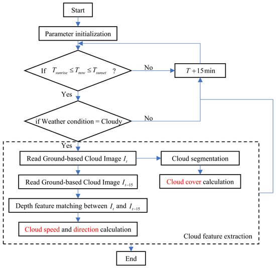
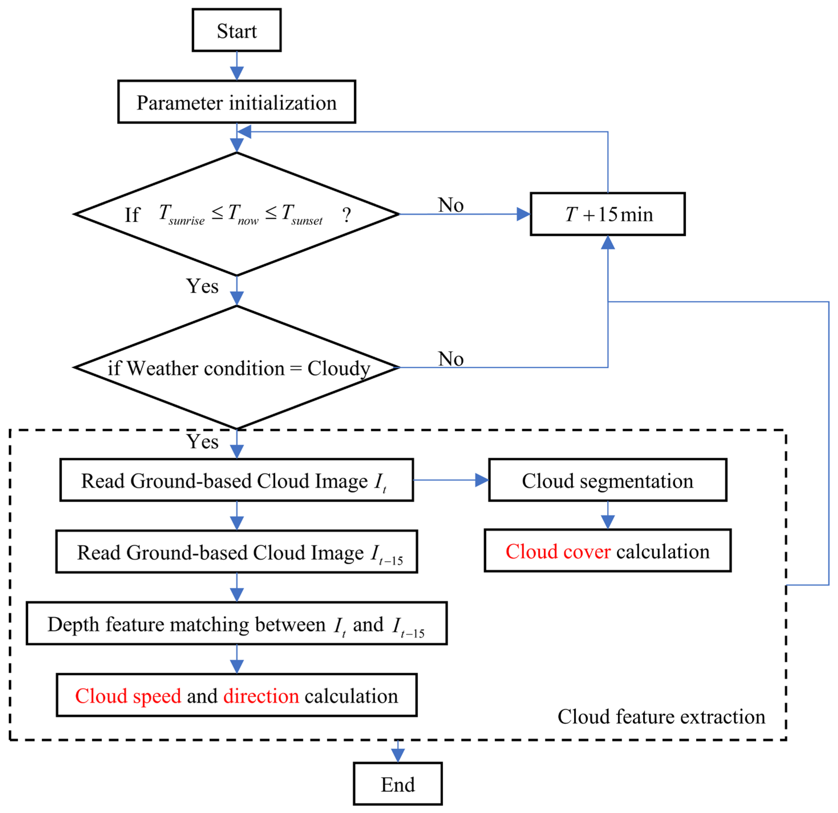
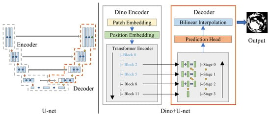
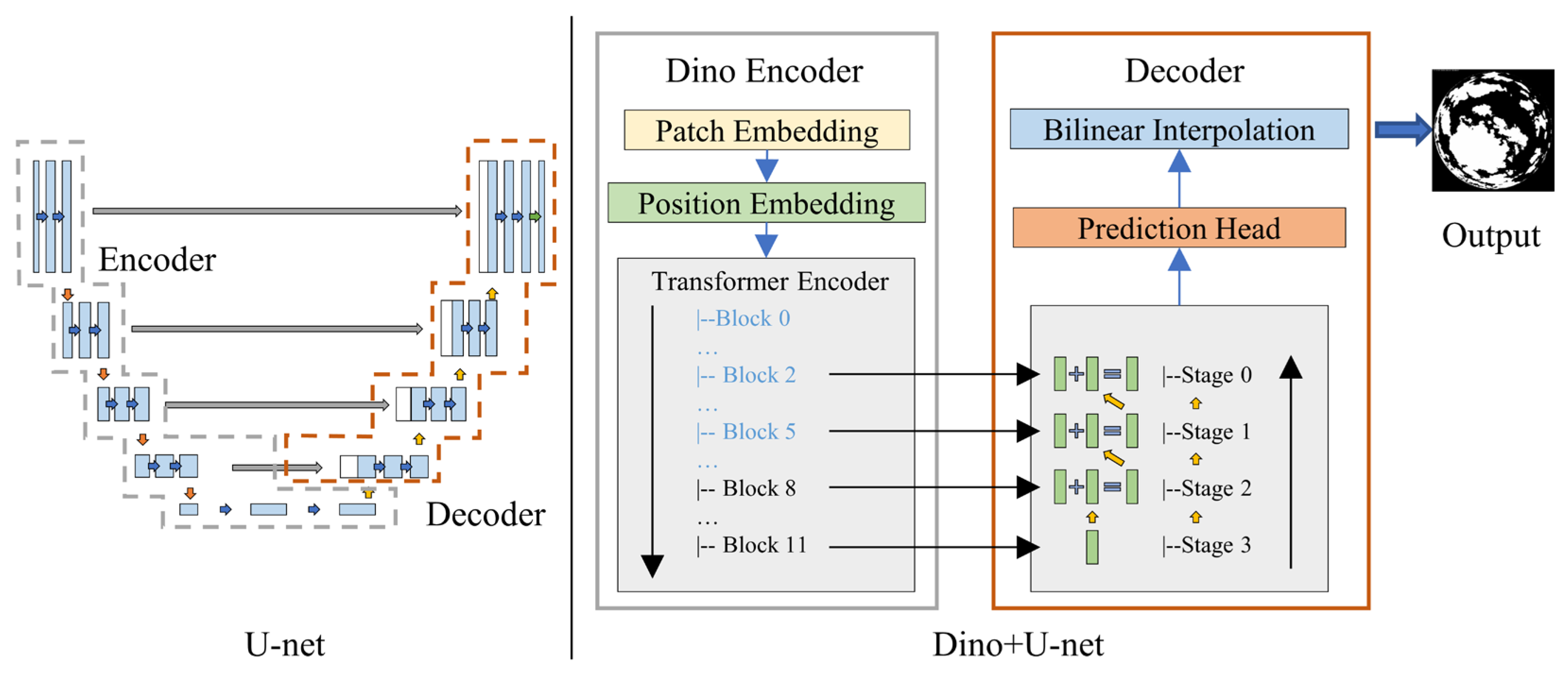
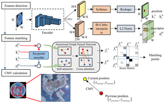
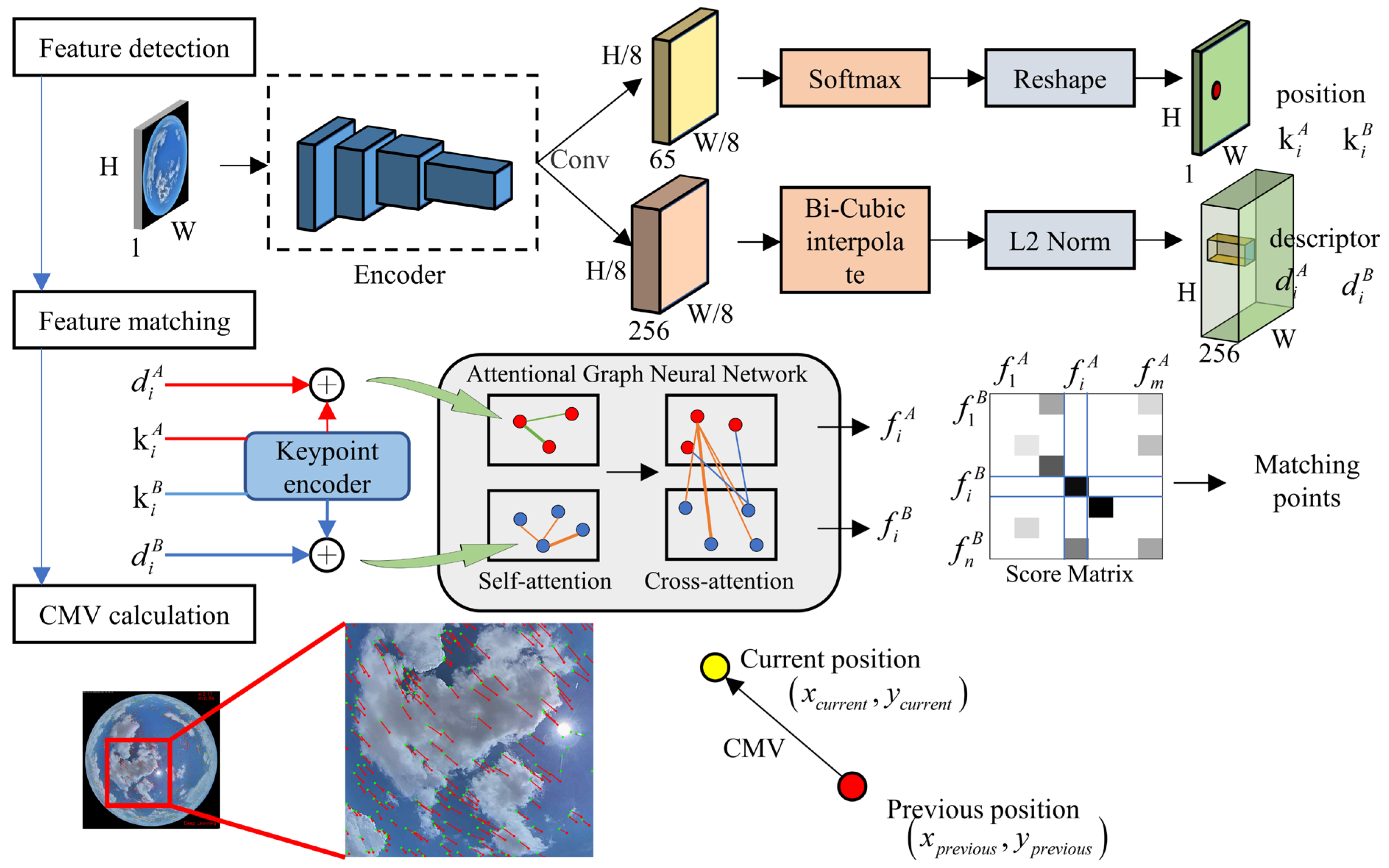
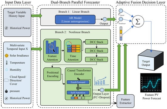
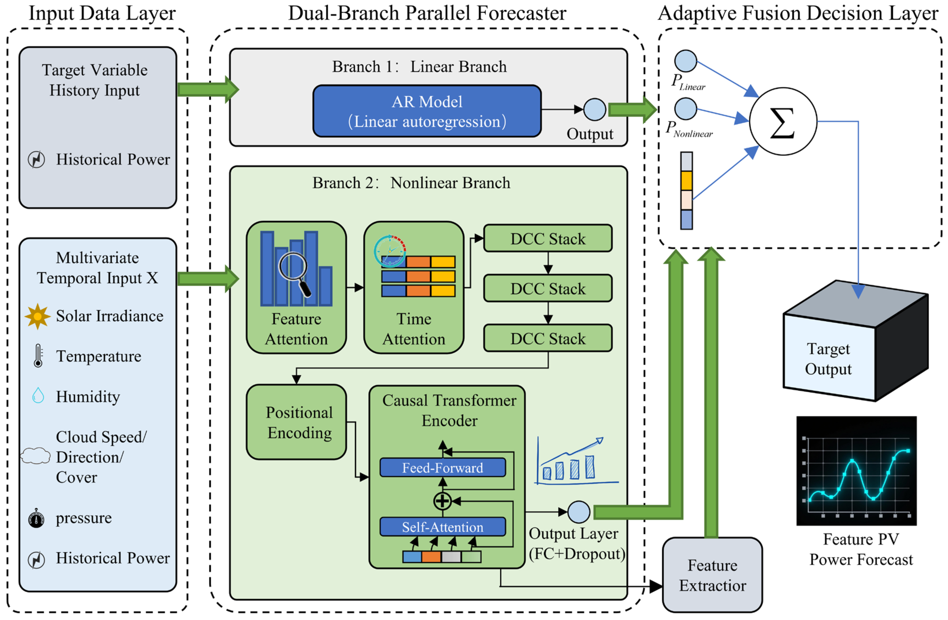
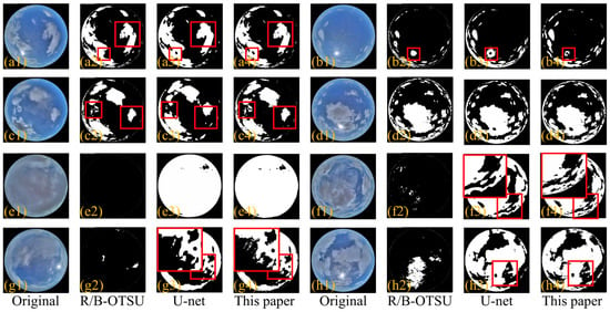
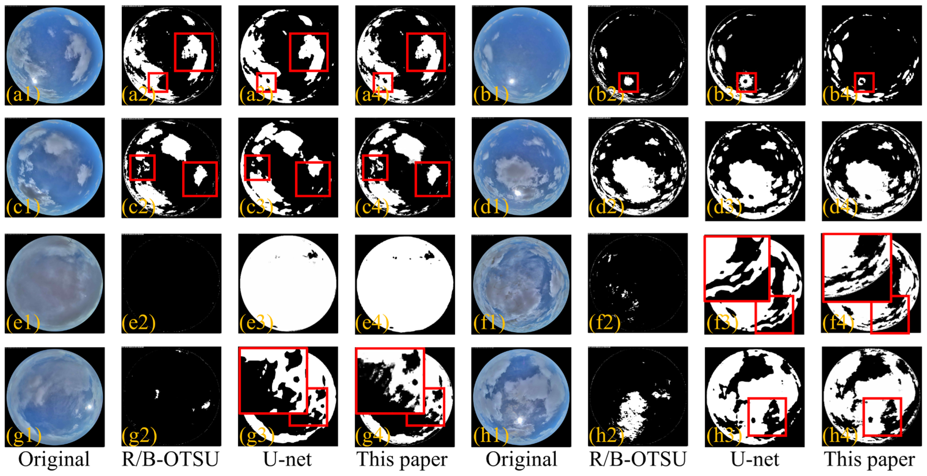
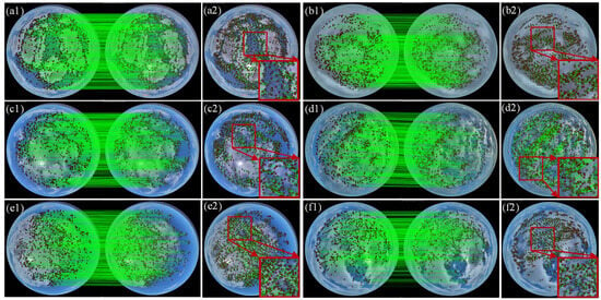
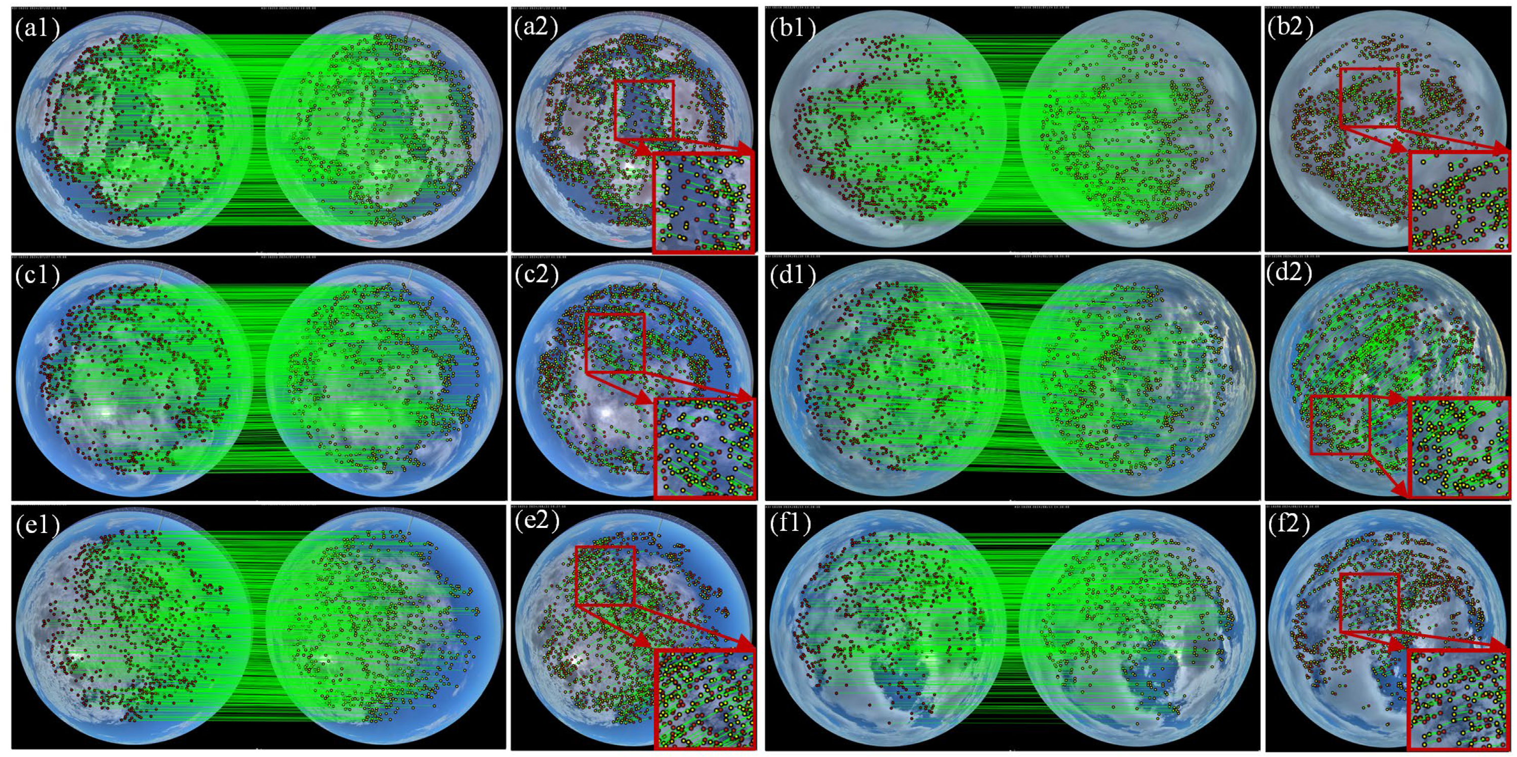
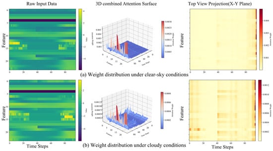
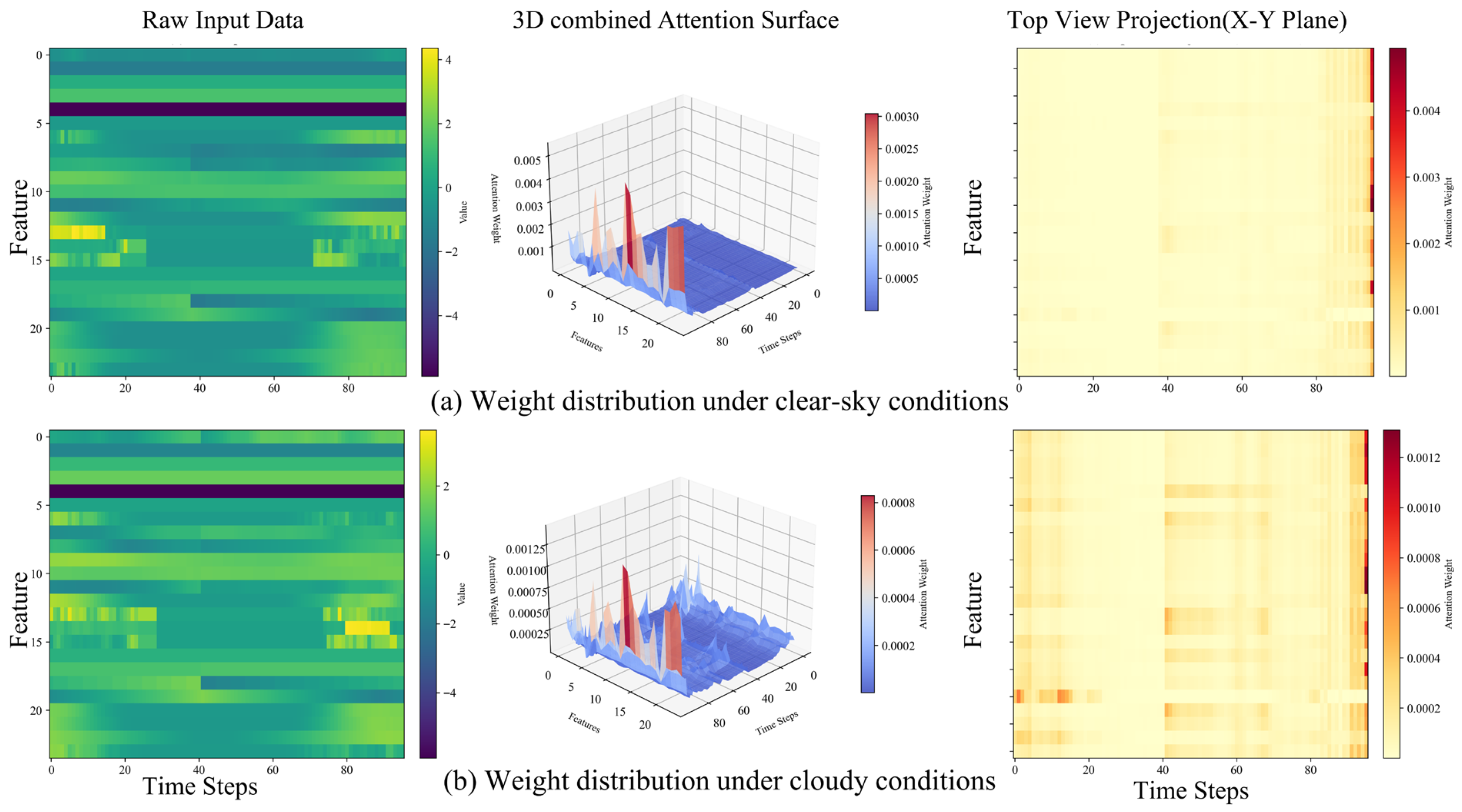
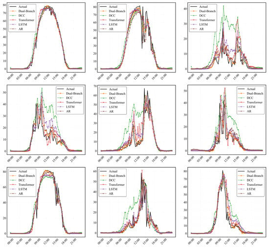
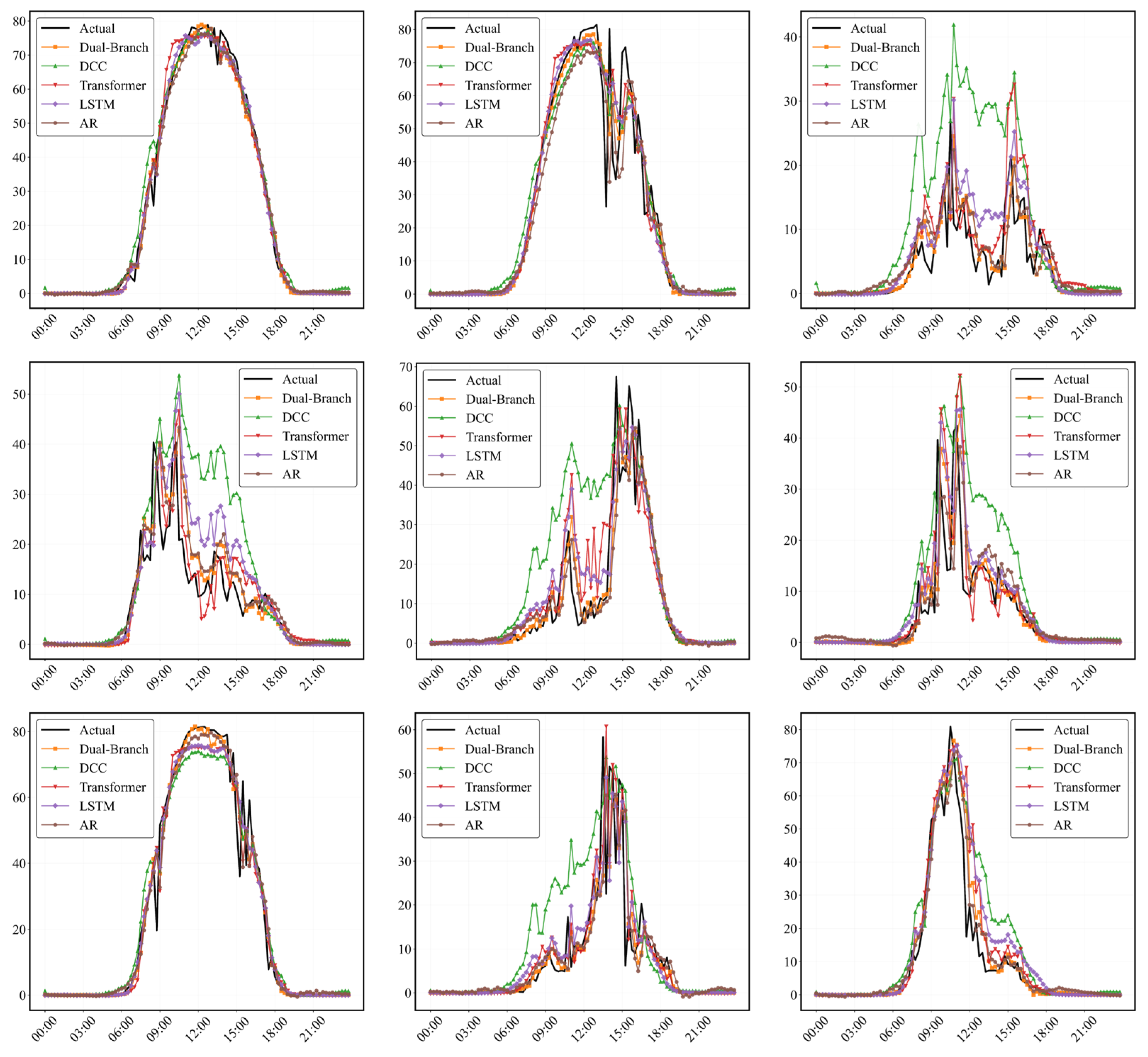
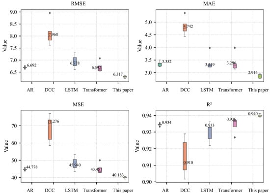
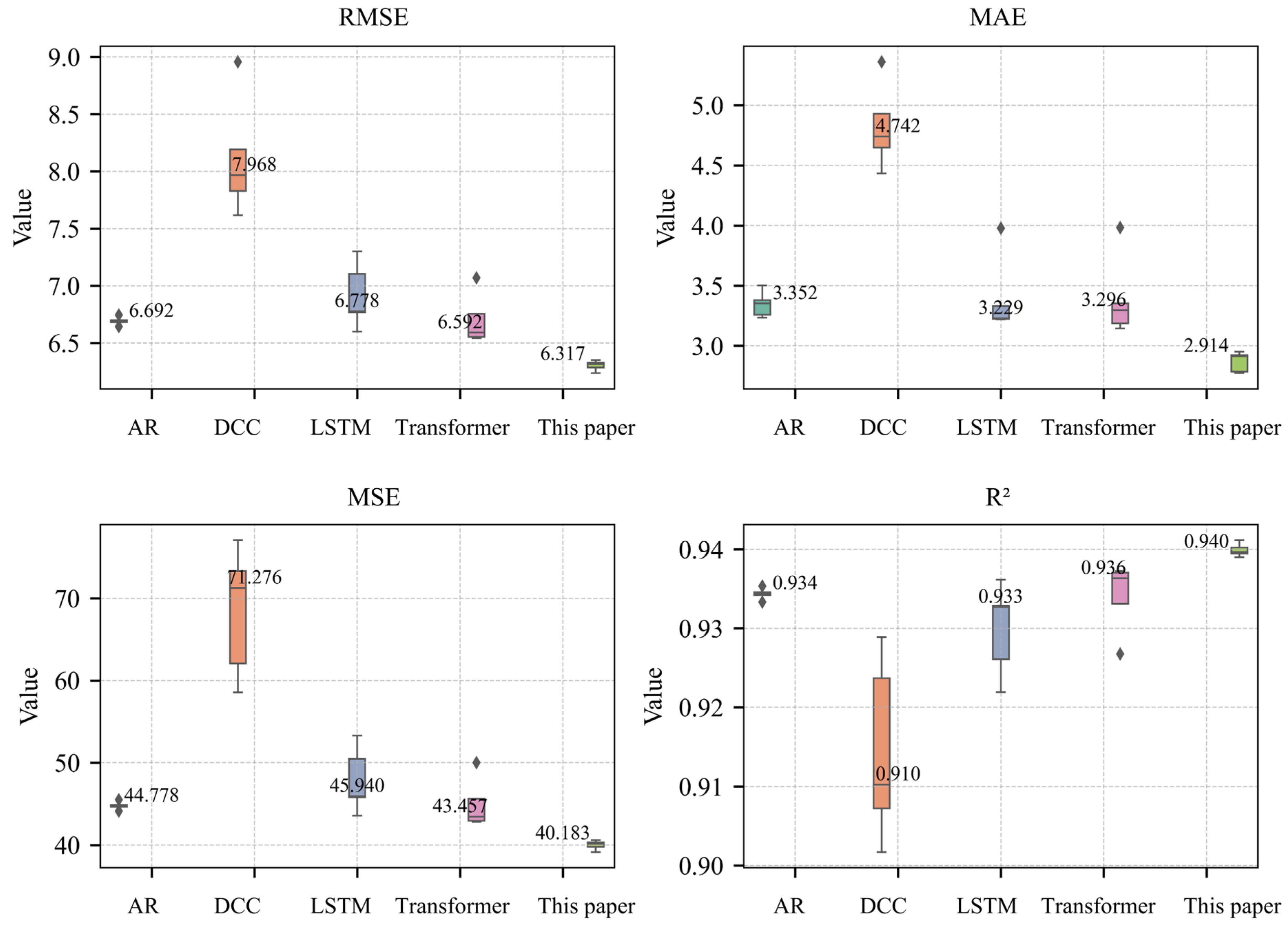

Disclaimer/Publisher’s Note: The statements, opinions and data contained in all publications are solely those of the individual author(s) and contributor(s) and not of MDPI and/or the editor(s). MDPI and/or the editor(s) disclaim responsibility for any injury to people or property resulting from any ideas, methods, instructions or products referred to in the content. |
© 2026 by the authors. Licensee MDPI, Basel, Switzerland. This article is an open access article distributed under the terms and conditions of the Creative Commons Attribution (CC BY) license.