Optimal Energy Storage Capacity Sizing Method Based on Power-Energy Characteristics of Curtailment and Deficit Events

Abstract

With the increasing penetration of renewable energy represented by wind and photovoltaic (PV) power in the power grid, the fluctuation amplitude of the net load curve is growing significantly, and the regulation capability of thermal power units can hardly accommodate such large fluctuations. When the adjustable range fails to meet the net load fluctuations, power curtailment and deficit issues arise in the system. Deploying energy storage is a common method to addressing power curtailment and deficit. However, over-sizing the storage capacity leads to low utilization of the storage equipment, while under-sizing fails to effectively mitigate the curtailment and deficit issues. Addressing the insufficiency of regulation capacity in future power systems with high wind and solar penetration, this paper proposes an optimal energy storage capacity allocation method based on the characteristics of power curtailment and deficit. First, a characterization model for the regulation capacity of existing conventional power sources is constructed. Combined with the annual wind and PV output curves, the temporal distribution of annual curtailment and deficit events is quantified based on the existing regulation capacity. Second, an optimal energy storage capacity allocation method matching the power–energy characteristics of curtailment and shortage is developed to minimize storage investment and maximize the reduction in losses caused by curtailment and deficit. Finally, the proposed method is validated based on a full-cycle operation scenario of a provincial power grid. The results show that compared with traditional empirical sizing schemes, the proposed scheme increases the complete mitigation rate of curtailment and deficit events from 32.57% to 49.01%; compared with the extreme sizing scheme that completely covers the gaps, it avoids a massive investment of nearly 380 million RMB/year. In future scenarios with gradually increasing renewable energy penetration, both the optimal charge/discharge duration and the event mitigation rate derived by the proposed scheme increase steadily, demonstrating its significant guiding value for long-term planning.

1. Introduction

With the deepening of the global energy transition, the penetration of renewable energy represented by wind and PV power continues to climb in power systems. The grid integration of renewable energy generation in China has experienced rapid development, with the installed capacity of wind and PV power continuously increasing. However, the output of renewable energy sources such as wind and solar power is highly variable. Their large-scale grid integration not only exacerbates the peak-shaving pressure on the system but also impacts the security and economy of traditional power system operations [1,2]. During intra-day operations, the system net load curve presents a steep “duck curve” characteristic [3,4]. Due to the rigid constraints on the maximum/minimum output and ramp rates of conventional thermal power units [5,6], the system’s regulation capacity struggles to fully track the net load fluctuations.

Deploying energy storage is a critical means to smooth out fluctuations [7,8]. However, the sizing of energy storage capacity faces rigorous technical and economic planning constraints [9,10]. Over-sizing the capacity leads to long-term equipment idling and wasted investment, while under-sizing fails to effectively alleviate the peak-shaving pressure of the power grid [11]. Therefore, optimizing the energy storage sizing scheme has become one of the core challenges for power grids with high renewable penetration.

Extensive research has been conducted by domestic and international scholars on the optimal sizing of energy storage capacity in power systems with high renewable energy penetration.

In terms of mitigating renewable energy fluctuations and improving system economy, references [12,13] explored energy storage capacity sizing methods to relax the peak-shaving bottlenecks of wind power integration, reducing the curtailment rate by absorbing surplus wind power during off-peak periods; references [14,15] proposed optimal siting and sizing strategies for distributed energy storage in distribution networks and islanded microgrids; references [16,17] constructed economic optimization models aiming to minimize the life-cycle cost of energy storage or the comprehensive system operation cost. However, the aforementioned studies mostly conduct macro-level capacity sizing based on daily electricity or full-cycle total energy, ignoring the discrepancy between power and energy in actual demand, which leads to the final configurations deviating from the actual demand of the power grid.

Regarding risk-based capacity sizing for the supply and demand uncertainty of high-proportion renewable energy, references [18,19] constructed two-stage robust optimal sizing models for energy storage based on extreme wind power fluctuations; references [20,21] explored chance-constrained and probabilistic forecasting planning methods considering the randomness of flexible supply and demand; references [22,23,24] further combined the Wasserstein metric with stochastic programming theory to establish energy storage dispatch and sizing models under worst-case scenarios. The above studies mostly rely on manual presetting when defining extreme scenarios and uncertainty sets, and thus cannot objectively identify the boundary where actual grid fluctuations deteriorate sharply, which tends to cause the optimization models to over-allocate capacity.

Regarding the multi-timescale coordination between energy storage and conventional units, references [25,26] established rolling optimal dispatch models incorporating demand-side response and multi-timescale source-storage-load coordination; references [27,28] evaluated the game mechanisms of battery energy storage participating in frequency regulation ancillary services and capacity pricing; references [29,30,31] proposed flexibility envelope models and joint wind-solar-storage optimization architectures. Although these methods explore aggregation models of multi-timescale resources, they do not satisfy the adaptive matching requirement for the charging/discharging duration of energy storage, thus violating the inherent duration distribution of grid deficits.

To address the theoretical deficiencies of the aforementioned methods, this paper proposes an optimal energy storage capacity sizing method based on the power-energy characteristics of power curtailment and deficit events. The main contributions of this paper are as follows:

• Construct an independent event characterization model to authentically restore the pulse-like shocks experienced by the system, thereby establishing a non-linear decoupling mechanism between power and energy.
• Utilize the Kneedle algorithm [32] to optimize the empirical cumulative distribution function (CDF) of independent events, constructing the capacity value boundary for energy storage configuration and eliminating the impact caused by extreme events.
• Establish a “power-energy” two-dimensionally decoupled global economic synergistic optimization model, taking the physical knee-points as feasible domain constraints, and solving for the global configuration parameters through a two-dimensional grid search.

The remainder of this paper is organized as follows: Section 2 establishes the daily regulation envelope and the benchmark unit commitment model for thermal power units. Section 3 completes the identification and quantification of power curtailment and deficit events. Section 4 derives the energy storage sizing method based on physical knee-points and economic synergy. Section 5 conducts case studies and multi-scheme comparisons based on data from a provincial power grid. Section 6 concludes the paper.

2. Regulation Capacity Envelope and Baseline Committed Capacity

2.1. Definition and Characteristics of Net Load

Given the original total system load L(t), wind power output W(t), and photovoltaic output S(t), the net load L_net(t) is defined as the residual demand after deducting the wind and PV power outputs from the total load:

L_net(t) = L(t) − W(t) − S(t)

(1)

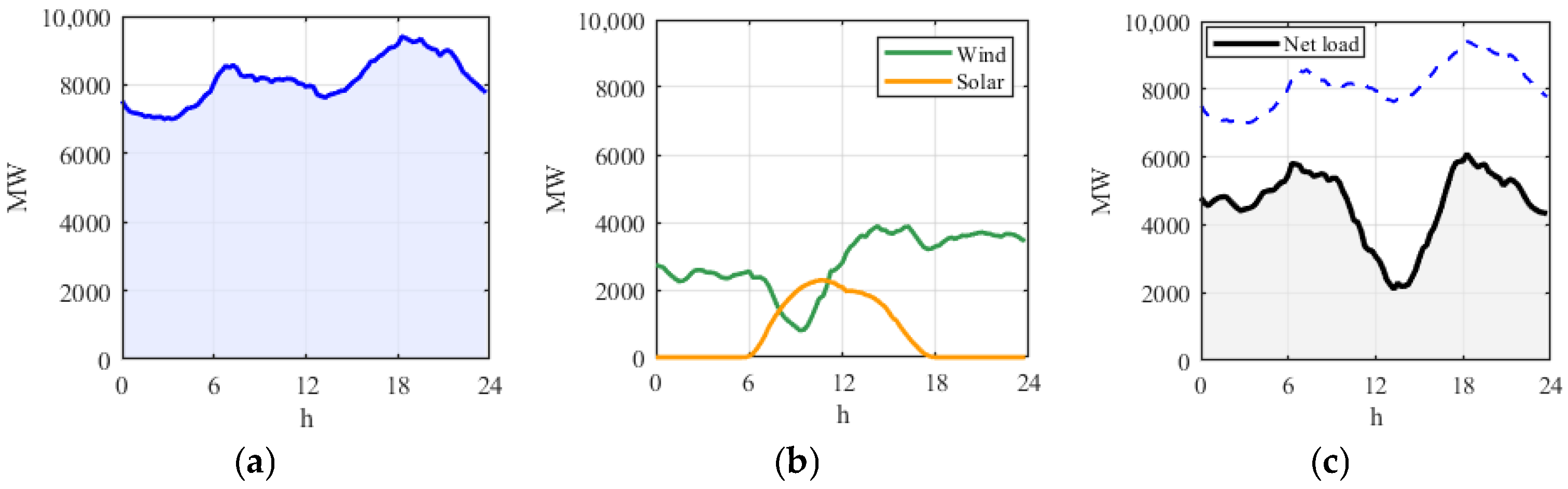
The net load represents the operational baseline that conventional generating units in the system must satisfy. Taking a typical day as an example, Figure 1 illustrates the evolution mechanism of the original load, wind and PV power outputs, and the net load curve.

As shown in Figure 1a, the traditional original load typically presents a double-peak pattern in the morning and evening. Figure 1b displays the intra-day distribution characteristics of renewable energy output: wind power tends to fluctuate throughout the entire day, whereas PV output exhibits strong temporal concentration, peaking at noon.

By superimposing these components to obtain the net load curve, Figure 1c clearly illustrates the morphological differences between the original load and the net load. Influenced by strong PV output, the net load curve is significantly depressed during the midday period, forming a typical deep valley; during the evening period, the sudden drop in PV output coupled with the surge in evening peak power consumption results in an extremely steep upward ramping trend for the net load.

These fluctuations, induced by renewable energy grid integration, constitute the core problem in the operation of high-penetration power grids: the regulation capacity of conventional thermal power units struggles to meet such severe net load fluctuations.

2.2. Definition of Regulation Capacity

To facilitate the analysis, it is assumed that all committed units have an identical rated capacity of P_rate. Given n committed units, the total committed capacity is S = n × P_rate. The actual adjustable power output of the units at any given moment is subject to the following three constraints:

• Capacity constraint. The maximum output of the units must not exceed the rated capacity, and spinning reserve must be retained to accommodate load forecast errors. Assuming the reserve ratio is β, the effective maximum output after deducting the reserve under load L(t) is S − βL(t).
• Minimum output constraint. Assuming a minimum output ratio of α, the total minimum output of the n units is αS; accounting for the downward spinning reserve, the effective minimum output is αS + βL(t).
• AGC regulation window constraint. Each unit has a rapid automatic generation control (AGC) regulation capability γ of approximately ±5% of the rated capacity around its operating base point. The total AGC regulation window of n units is γS. Therefore, from the current load base point L_net(t), the maximum achievable output upward is L_net(t) + γS, and the minimum achievable output downward is L_net(t) − γS.

Combining the above three constraints, the effective upper limit P_up(t) of thermal power output is:

P_up(t,n) = min(S − βL(t),L_net(t) + γS)

(2)

the effective lower limit P_lo(t) is:

P_lo(t,n) = max(αS + βL(t),L_net(t) − γS)

(3)

To avoid the dimensional explosion caused by introducing large-scale Mixed Integer Linear Programming (MILP) in full-year long-term planning, the envelope model in this paper adopts certain macroscopic equivalent simplifications. This macroscopic static envelope simplification may, to some extent, slightly overestimate the system’s actual dynamic ramping response capability, thereby making the calculated curtailment and deficit gaps somewhat conservative. However, at the level of long-term macroscopic capacity planning, this approximate model strikes a reasonable balance between computational efficiency and the characterization of system physical boundaries.

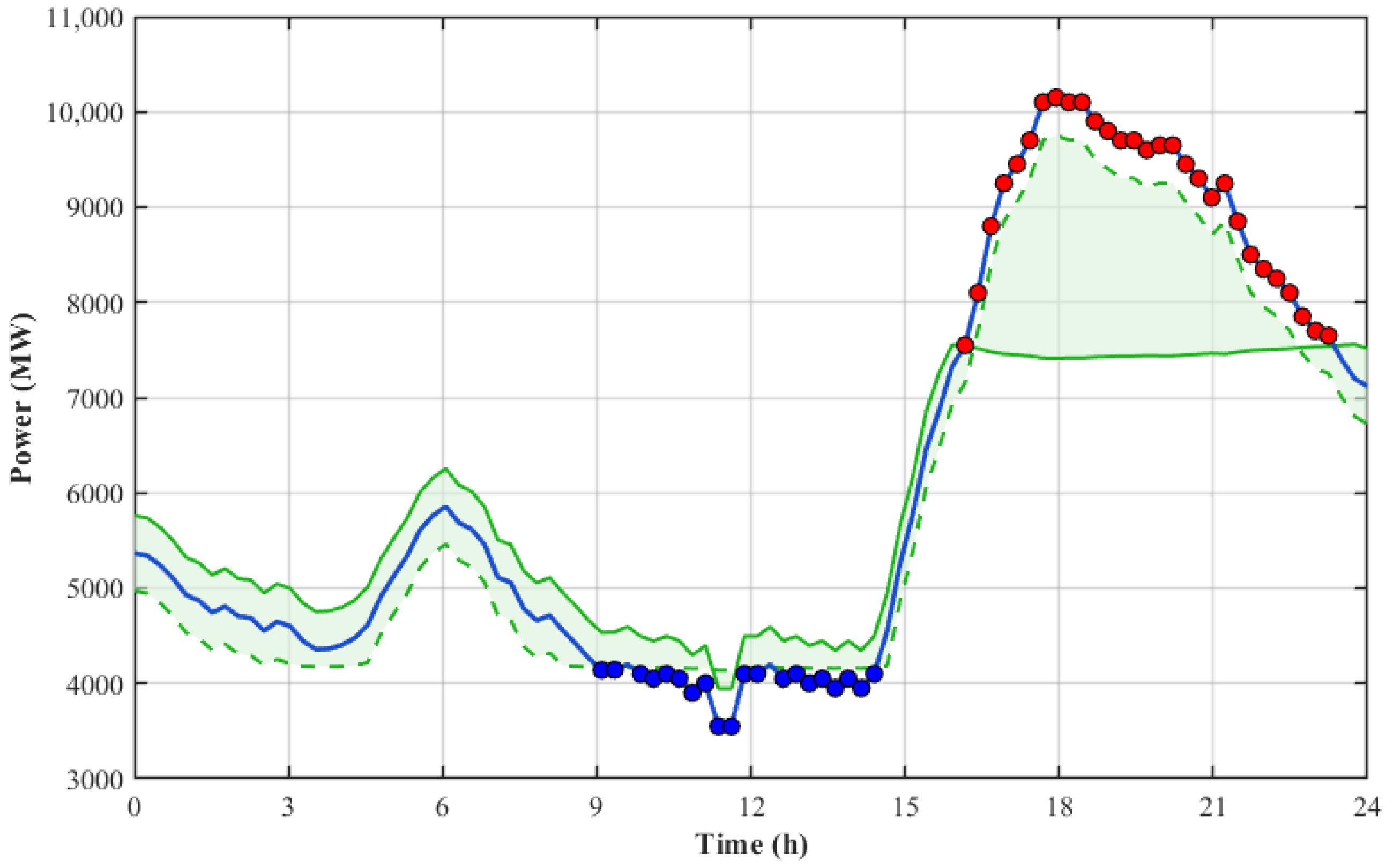
Therefore, for given time t and number of committed units n, the interval [P_lo(t,n), P_up(t,n)] constitutes the regulation capacity envelope of the thermal power units. Figure 2 presents a comparison between the regulation capability interval of thermal power units and the net load curve under a certain scheme. The green region represents the adjustable output range of thermal power units, with the green solid line denoting the upper boundary P_up(t), the green dashed line denoting the lower boundary P_lo(t), the blue curve denoting the net load, and the red and blue scatter points denoting the net load fluctuations that cannot be accommodated by the regulation capability.

During certain periods, the upper and lower boundaries of the regulation capacity region may become inverted, which indicates the complete exhaustion of the regulation capacity of conventional units under the current committed capacity. When the mismatch between the net load and the current committed capacity is too large, thermal power units, even at their physical limits, cannot simultaneously satisfy the minimum output/maximum capacity constraints and the AGC regulation reserve requirements.

When the committed capacity S is insufficient relative to the net load L, i.e., S < (1 + β)L, the effective upper limit P_up is dominated by S − βL, and the effective lower limit P_lo is dominated by L − γS. In this case, P_up is much smaller than P_lo, indicating that even operating at full capacity, the units cannot meet the net load at this moment.

When the committed capacity S is excessively large relative to the net load L, i.e., S > (1 − β)L ∕ α, the effective lower limit P_lo is dominated by αS + βL, and the effective upper limit P_up is dominated by L + γS. In this case, P_lo is greater than P_up, indicating that even when reduced to their minimum output, the units still exceed the net load at this moment.

From the above analysis, the feasible window of net load corresponding to a given committed capacity S can be derived as:

$${\displaystyle \frac{\mathit{\alpha S}}{1-\beta }}\le L(t)\le {\displaystyle \frac{S}{1+\beta }}$$

(4)

In the quantitative framework of this paper, fluctuations exceeding the feasible window of net load represent the portion that cannot be accommodated by the regulation capacity of thermal power units, necessitating the additional deployment of energy storage to smooth out such fluctuations.

2.3. Determination of Baseline Committed Capacity

The envelope coverage rate (CR) of the thermal power units’ regulation capacity characterizes the proportion of time during which the units, under a specific committed capacity, can achieve supply–demand balance solely by relying on their own upper and lower regulation limits, without triggering external interventions (such as power curtailment, load shedding, or energy storage dispatch).

For day d and the number of committed units n, the daily coverage rate is defined as follows:

$$C{R}_d(n)={\displaystyle \frac{1}{T_{\mathit{total}}}}{\displaystyle \sum _{t=1}^{T_{\mathit{total}}}\mathbb{I}}\left[P_{\mathit{lo}}(t,n)\le L_{\mathit{net},d}(t)\le P_{\mathit{up}}(t,n)\right]$$

(5)

where CR_d(n) is the envelope coverage rate on day d with n committed units; T_total is the total number of time steps in a single day; $\mathbb{I}$ is the indicator function, which equals 1 when the logical condition inside the brackets holds (i.e., the net load at time t does not cross the boundaries and strictly falls within the adjustable range of the thermal power units), and 0 otherwise; P_lo(t,n) and P_up(t,n) represent the effective lower and upper boundaries of the thermal power units at time t, respectively; and L_net,d(t) is the system net load at the corresponding time.

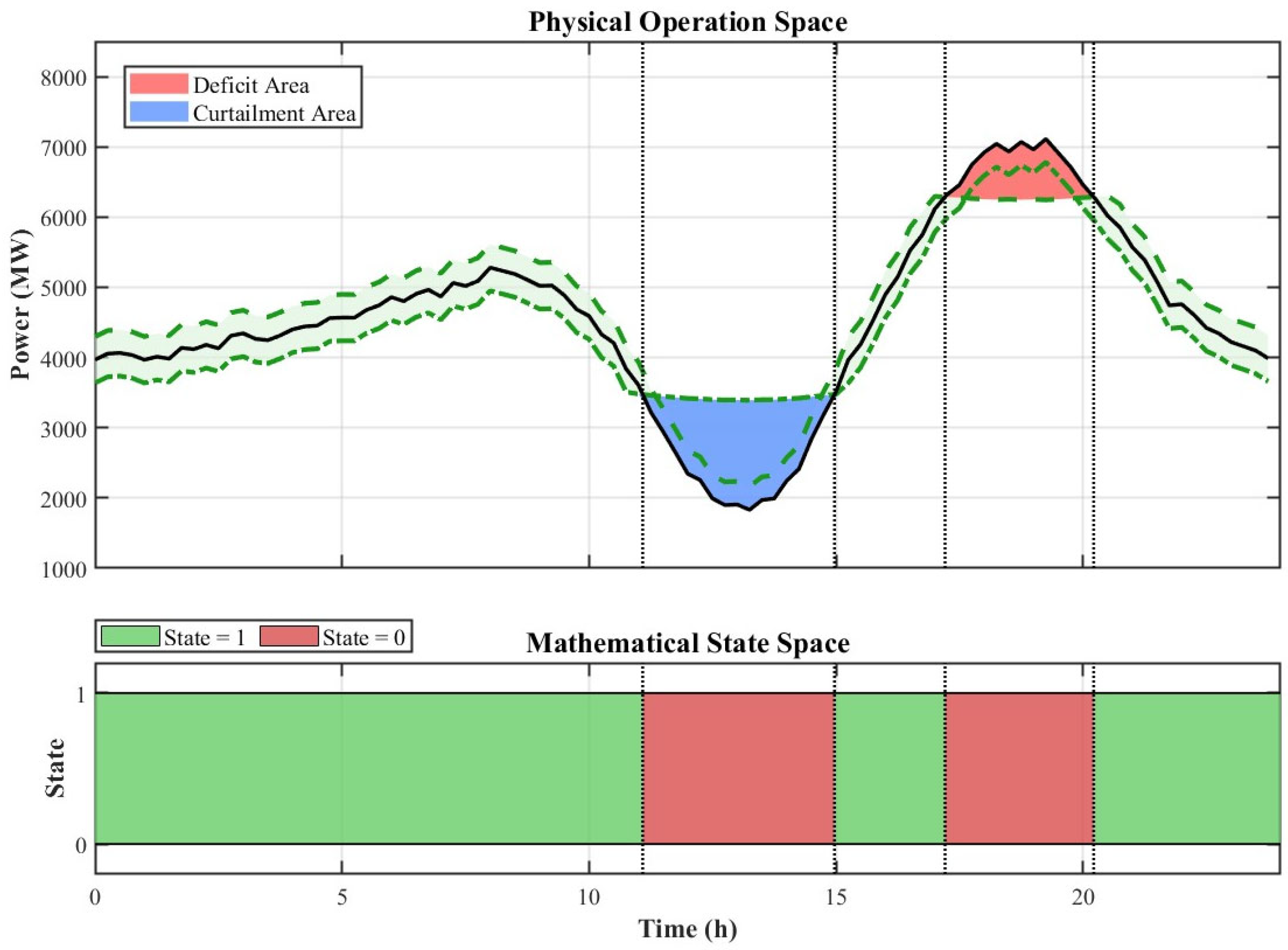
An illustrative example of the time status for a specific day is shown in Figure 3:

As illustrated in Figure 3, the upper subplot represents the unit operating status, demonstrating the geometric overlapping relationship between the system net load and the thermal power regulation capacity. The lower subplot depicts the mathematical state space, illustrating the downward projection mapping of the indicator function $\mathbb{I}$[⋅] along the time axis.

When the net load strictly falls within the regulation capacity interval, the logical condition of the indicator function holds true, outputting a state value of 1, which projects downward as a green time rectangle. Conversely, when the regulation capacity of the thermal power units fails to accommodate the net load fluctuations, the indicator function undergoes a step change and outputs a state value of 0, projecting downward as a red time rectangle.

In summary, the coverage rate CR_d(n) essentially represents the proportion of the green state duration relative to the total daily operating time in the projection diagram. Based on this evaluation metric, this paper takes maximizing the coverage rate as the surrogate objective to search the feasible range of committed units for the optimal daily number of committed units $n_d^{*}$. In practical decision-making, if multiple commitment schemes achieve the same maximum coverage rate, the scheme with the minimum committed capacity is selected as the final daily decision.

3. Curtailment and Deficit Events

After the daily baseline unit commitment scheme is determined, the upper and lower boundaries of the thermal power units’ regulation capacity are subsequently established. At this point, the portions of the net load curve that fall outside the regulation capacity envelope represent the flexibility gaps that the system cannot self-regulate relying solely on internal conventional units, namely, the power curtailment and deficit events. This section will rigorously identify and quantify these deficit and curtailment events.

3.1. Definition of Curtailment and Deficit Events

Deficit events occur at moments when the system’s upward regulation capacity is exhausted. The deficit power is defined as the portion of the net load that exceeds the effective upper limit of the thermal power output:

$$P_{\mathit{def}}(t)=\max (0,L_{\mathit{net}}(t)-P_{\mathit{up}}(t,n_d^{*}))$$

(6)

Assuming a total of M_def deficit events occur throughout the year, the occurrence period for the i-th deficit event is denoted as $\left[t_{s,i}^{\mathit{def}},t_{e,i}^{\mathit{def}}\right]$, and its maximum peak power $P_{\mathit{peak},i}^{\mathit{def}}$ is given by:

$$P_{\mathit{peak},i}^{\mathit{def}}=\underset{t\in \left[t_{s,i}^{\mathit{def}},t_{e,i}^{\mathit{def}}\right]}{\max }{P}_{\mathit{def}}(t)$$

(7)

By performing discrete integration of the deficit power along the time axis, the cumulative deficit energy $E_{\mathit{event},i}^{\mathit{def}}$ of this deficit event can be quantified as:

$$E_{\mathit{event},i}^{\mathit{def}}={\displaystyle \sum _{t=t_{s,i}^{\mathit{def}}}^{t_{e,i}^{\mathit{def}}}{P}_{\mathit{def}}(t)}\cdot \Delta t$$

(8)

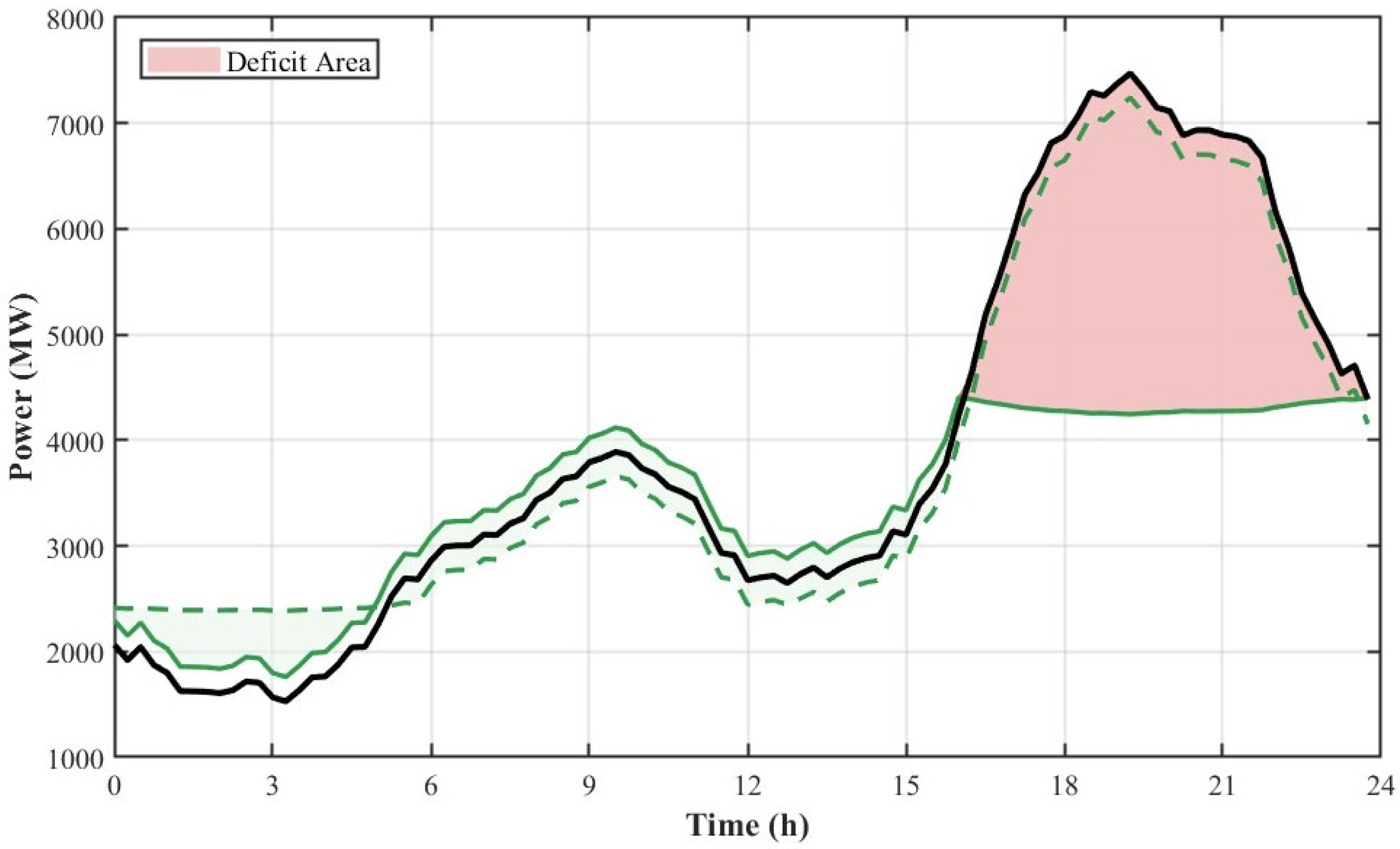
where Δt is the time resolution step size. A typical scenario is extracted in this paper to plot the schematic diagram of the deficit area, as shown in Figure 4.

As illustrated in Figure 4, when the evening peak load surges or the wind and solar power outputs drop suddenly, the net load curve penetrates upward through the upper boundary of the regulation capacity. The red area in the figure represents the system’s “upward flexibility gap” that cannot be accommodated by thermal power units. The integral area of this region corresponds to the daily deficit energy, and this energy gap needs to be smoothed out by discharging external energy storage devices.

Symmetrically, curtailment events occur at moments when the system’s downward regulation capacity is exhausted. The curtailment power is defined as the portion by which the effective lower limit of the thermal power output exceeds the net load:

$$P_{\mathit{cur}}(t)=\max (0,P_{\mathit{lo}}(t,n_d^{*})-L_{\mathit{net}}(t))$$

(9)

Assuming a total of M_cur curtailment events occur throughout the year, the occurrence period for the j-th curtailment event is denoted as $\left[t_{s,j}^{\mathit{cur}},t_{e,j}^{\mathit{cur}}\right]$, and its maximum peak power $P_{\mathit{peak},j}^{\mathit{cur}}$ is given by:

$$P_{\mathit{peak},j}^{\mathit{cur}}=\underset{t\in \left[t_{s,j}^{\mathit{cur}},t_{e,j}^{\mathit{cur}}\right]}{\max }{P}_{\mathit{cur}}(t)$$

(10)

Similarly, by performing discrete integration of the curtailment power, the cumulative curtailment energy $E_{\mathit{event},j}^{\mathit{cur}}$ of this curtailment event can be quantified as:

$$E_{\mathit{event},j}^{\mathit{cur}}={\displaystyle \sum _{t=t_{s,j}^{\mathit{cur}}}^{t_{e,j}^{\mathit{cur}}}{P}_{\mathit{cur}}(t)}\cdot \Delta t$$

(11)

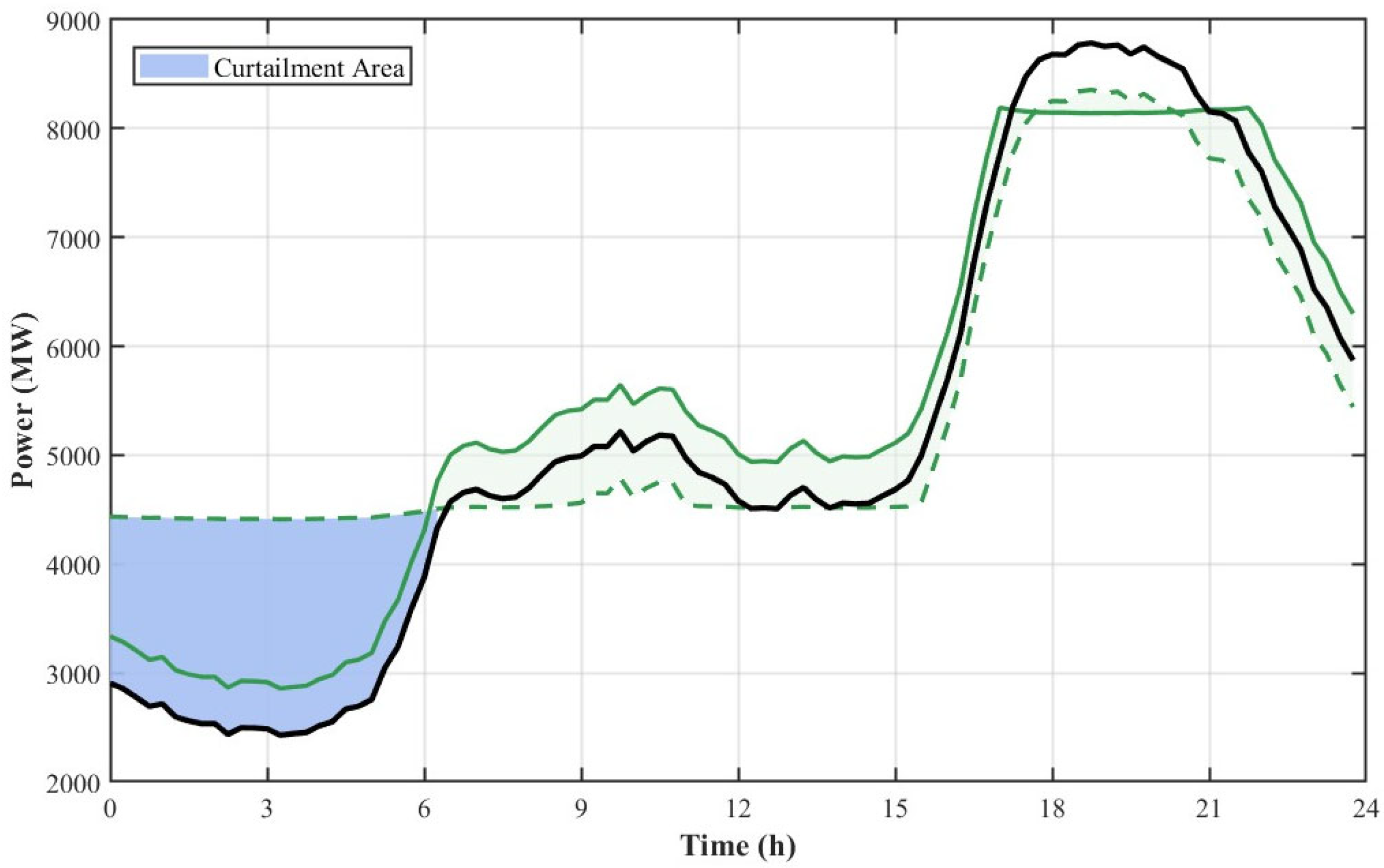
A typical scenario is extracted to plot the schematic diagram of the curtailment area, as shown in Figure 5:

As illustrated in Figure 5, during periods of high photovoltaic generation or wind power surges, the net load curve is depressed below the lower boundary of the thermal power regulation capacity. The blue area in the figure represents the “downward flexibility gap” that cannot be accommodated by the units. The integral area of this region corresponds to the curtailed energy, and this surplus energy constitutes a natural energy pool for charging the energy storage devices.

3.2. Temporal Distribution and Sorted Characteristics of Events

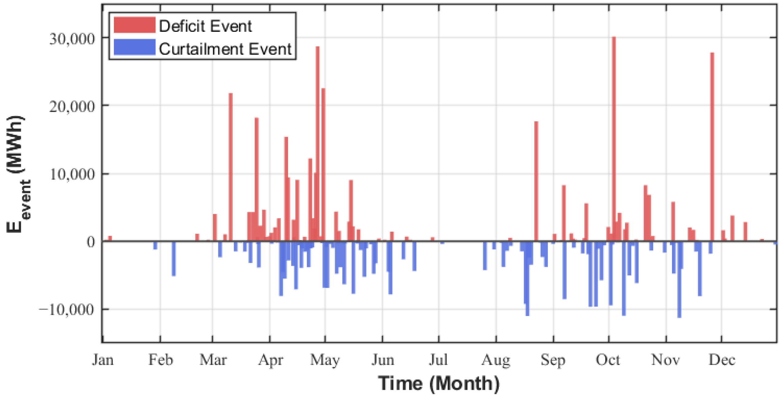
After identifying and quantifying the curtailment and deficit events, these values can be plotted along the time axis to reveal the temporal distribution characteristics of the system’s flexibility gaps, as illustrated in Figure 6.

Due to the strong meteorological correlation of renewable energy output and the socio-economic attributes of load demand, the system’s flexibility gaps often exhibit significant seasonal alternation and spatiotemporal clustering effects. For instance, in seasons characterized by high renewable generation but sluggish load demand, the system’s downward regulation capacity is easily exhausted, leading to frequent occurrences of continuous power curtailment. Conversely, during periods of extreme temperatures coupled with low wind speeds, the upward regulation capacity is often insufficient, thereby triggering power deficit events.

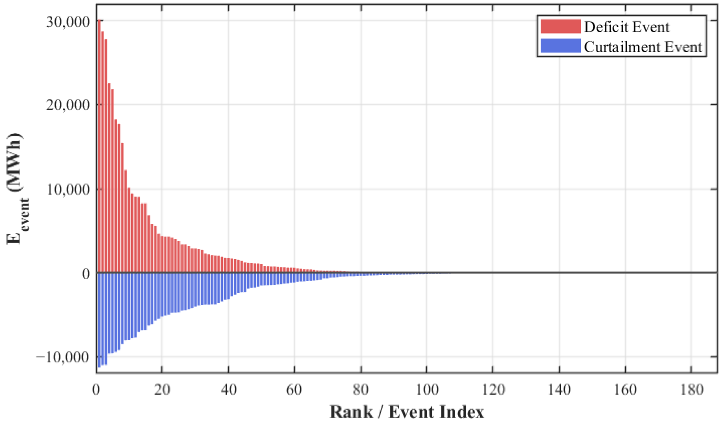
By sorting these sequences in descending order of magnitude, the “curtailment/deficit duration curve” is constructed. The deficit and curtailment sequences are independently re-indexed from the largest to the smallest values to obtain monotonically decreasing sorted sequences.

As illustrated by the geometric morphology in Figure 7, the sorted curtailment and deficit duration curves of the high-proportion renewable energy power grid exhibit typical extreme skewness and “heavy-tail” characteristics. A few samples at the very beginning of the curves present extremely high magnitudes, implying that a very small number of extreme days contribute to the vast majority of the system’s total curtailment and deficit energy. The latter segments of the curves converge rapidly and cling to the horizontal axis, indicating that during the overwhelming majority of days in the full cycle, the system’s net load fluctuations fall completely within, or only slightly exceed, the regulation capacity range of conventional units.

4. Energy Storage Capacity Sizing Method

By analyzing the temporal bar charts of curtailment and deficit events, the core dilemma faced by traditional energy storage sizing methods is elucidated: relying on a few extreme events as the sizing basis inevitably leaves the energy storage system idle for the vast majority of the year; conversely, under-sizing the capacity fails to mitigate the vast majority of curtailment and deficit events.

To address the challenge of rational energy storage capacity sizing, this chapter constructs an optimal sizing method that matches the power-energy characteristics of the curtailment and deficit events.

4.1. Over-Sizing and Under-Sizing of Energy Storage Capacity

Under daily operational scenarios, energy storage primarily functions as cross-time energy shifting: charging to store energy during curtailment periods and discharging to compensate for gaps during deficit periods. On the sorted duration curve of curtailment and deficit events, a given energy storage capacity E acts as a horizontal truncation line, demarcating the effective working zone of the energy storage.

Given the rated energy storage capacity E, the remaining deficit and curtailment energy uncovered by the energy storage are respectively given by:

$$E_{\mathit{unserved}}^{\mathit{def}}(E)={\displaystyle \sum _{i=1}^{M_{\mathit{def}}}\max (0,E_{\mathit{event},i}^{\mathit{def}}-E)}$$

(12)

$$E_{\mathit{unserved}}^{\mathit{cur}}(E)={\displaystyle \sum _{j=1}^{M_{\mathit{cur}}}\max (0,E_{\mathit{event},j}^{\mathit{cur}}-E)}$$

(13)

Equations (12) and (13) conceptually represents the cumulative sum of the residual energy from all independent events that exceeds the configured energy storage capacity E. Specifically, the max(0,∙) operator calculates the unmitigated overflow energy for a single event. If an individual event’s energy is less than or equal to the storage capacity E, it is fully mitigated by the energy storage, yielding zero residual. If it exceeds E, only the overflow portion is recorded.

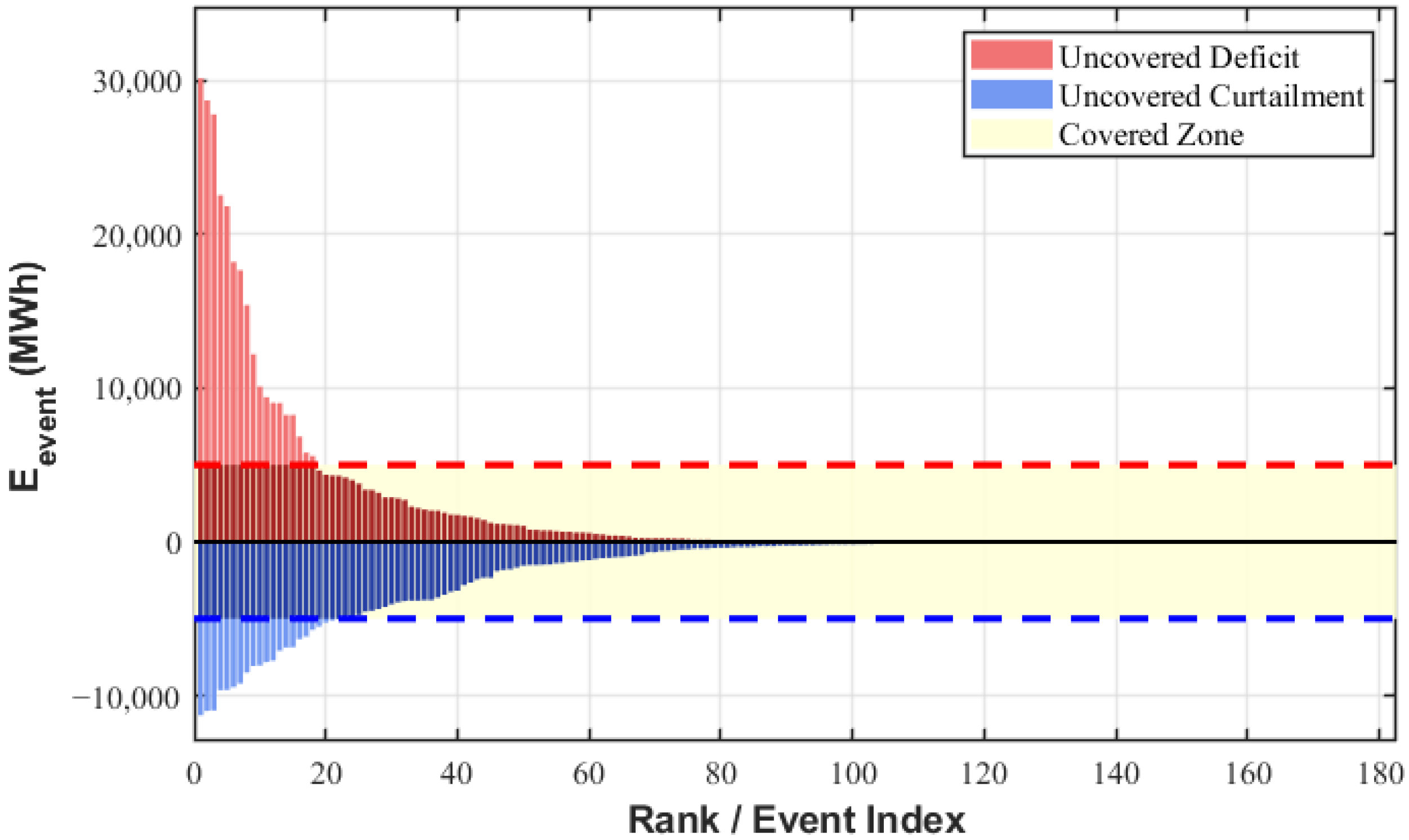
Taking E = 5000 MWh as an example, Figure 8 illustrates the energy storage capacity boundaries using horizontal lines at ±5000 MWh. Under this configuration, the energy storage covers approximately 50% of the deficit energy and 83% of the curtailed energy.

Observing Figure 8, it is evident that the width of the energy storage capacity envelope [−E,E] directly impacts the security and economy of the system. When the configured capacity is set at an extremely low level, it is termed capacity under-sizing. Assuming the penalty prices for power deficit and curtailment are r_def and r_cur respectively, the remaining penalty loss C_gap(E) under the under-sized state is formulated as:

$$C_{\mathit{gap}}(E)=r_{\mathit{def}}{\displaystyle {\displaystyle \sum _{i=1}^{M_{\mathit{def}}}}\max (0,E_{\mathit{event},i}^{\mathit{def}}-E)+r_{\mathit{cur}}}{\displaystyle {\displaystyle \sum _{j=1}^{M_{\mathit{cur}}}}\max (0,E_{\mathit{event},j}^{\mathit{cur}}-E)}$$

(14)

Conversely, if the configured capacity is forcibly elevated to an excessively high level to pursue power supply reliability, it results in capacity over-sizing. Let the unit energy investment cost and unit power investment cost of the energy storage system be c_e and c_p respectively, and the annualized discount factor be F. Assuming the system’s charge/discharge duration is rigidly fixed at 4 h, the investment cost function C_inv(E) can be expressed as:

$$C_{\mathit{inv}}(E)=F\cdot (c_p\cdot {\displaystyle \frac{E}{4}}+c_e\cdot E)$$

(15)

However, as the investment in energy storage equipment increases, its utilization rate drops drastically. The annualized life-cycle utilization rate of the energy storage system, η_util(E), is defined as the ratio of the total energy actually mitigated throughout the year to its theoretical maximum energy throughput:

$${\eta }_{\mathit{util}}(E)={\displaystyle \frac{{\displaystyle \sum _{i=1}^{M_{\mathit{def}}}\min (E_{\mathit{event},i}^{\mathit{def}},E)+{\displaystyle \sum _{j=1}^{M_{\mathit{cur}}}\min (E_{\mathit{event},j}^{\mathit{cur}},E)}}}{E\cdot (M_{\mathit{def}}+M_{\mathit{cur}})}}\times 100\%$$

(16)

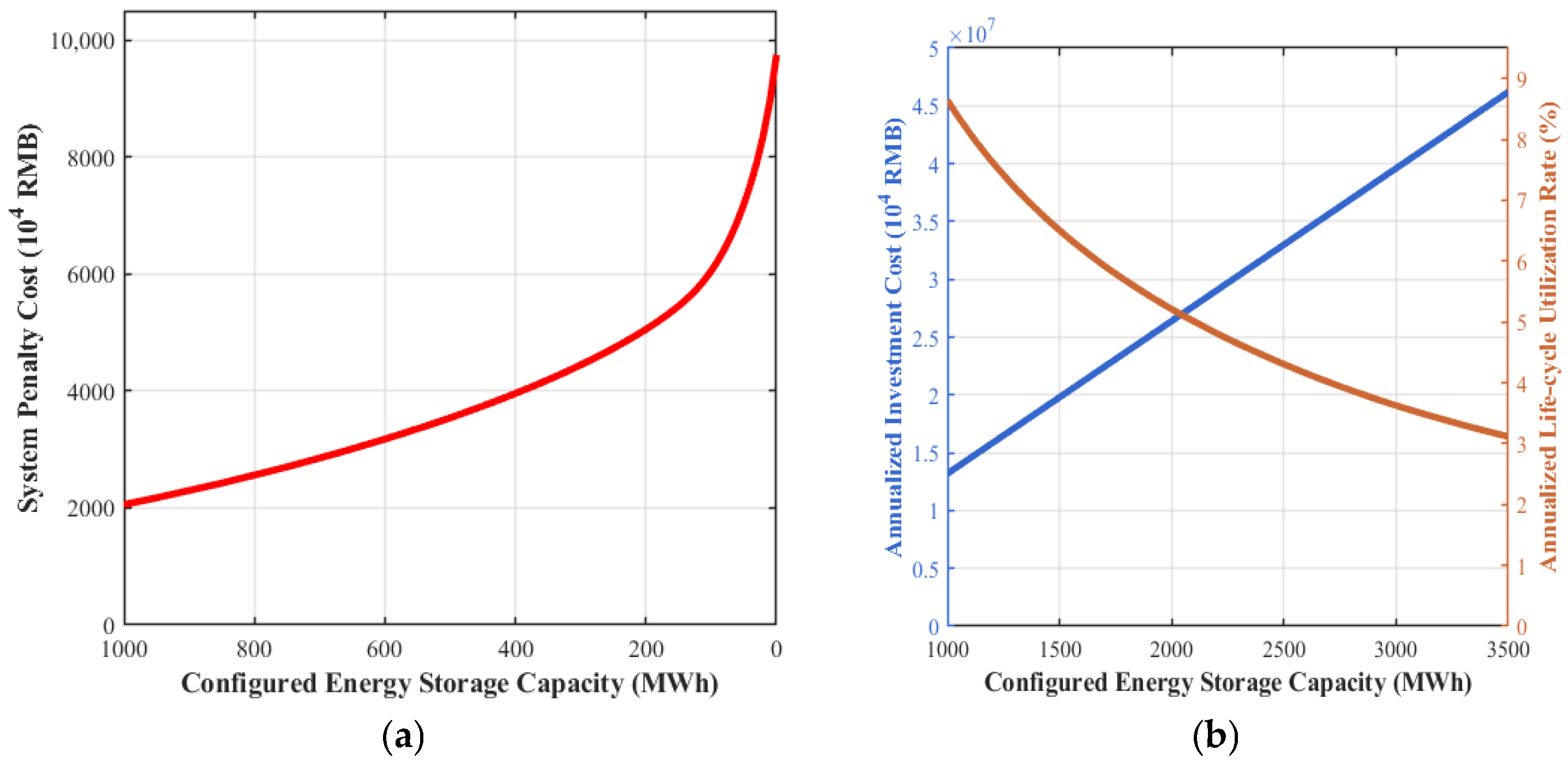
The evolutionary curves of economic characteristics under capacity under-sizing and over-sizing conditions are illustrated in Figure 9.

In the under-sizing region shown in Figure 9a, the system’s ability to smooth fluctuations diminishes significantly as the configured capacity is progressively compressed. During this process, the volume of deficit and curtailment energy exposed outside the energy storage envelope increases exponentially, driving the system’s comprehensive penalty cost curve to exhibit an extremely steep upward trend.

In the over-sizing region shown in Figure 9b, as the capacity is continuously pushed higher, the blue curve representing the annualized investment cost of the system rises linearly; in contrast, the orange curve representing the annualized equipment utilization rate undergoes a precipitous decline. This contrast reveals that blindly increasing energy storage capacity to cover extreme events with extremely low occurrence probabilities leads to a state where the vast majority of the newly added capacity remains idle throughout the year, thereby resulting in massive asset wastage and sunk costs.

4.2. Optimal Sizing Method for Energy Storage Capacity

Rational energy storage sizing should neither bear excessive penalty losses caused by under-sizing nor tolerate equipment idling and wastage resulting from over-sizing. This section analyzes the distribution patterns of annual power curtailment and deficit events in the “power-energy” two-dimensional plane. By combining the physical knee-points of the Cumulative Distribution Function (CDF) with a comprehensive economic objective function, we derive an energy storage sizing optimization scheme that balances physical support capability with economic rationality.

The configuration of the energy storage system involves both rated power P and rated capacity E. For the M_def deficit events and M_cur curtailment events occurring throughout the full cycle, the Cumulative Distribution Function (CDF) for the peak power and cumulative energy of these two types of events is constructed respectively. Here, CDF statistically describes the probability that a random variable takes on a value less than or equal to a specific threshold:

$$F_P^{\mathit{def}}(P)={\displaystyle \frac{1}{M_{\mathit{def}}}}{\displaystyle \sum _{i=1}^{M_{\mathit{def}}}\mathbb{I}}(P_{\mathit{peak},i}^{\mathit{def}}\le P)$$

(17)

$$F_E^{\mathit{def}}(E)={\displaystyle \frac{1}{M_{\mathit{def}}}}{\displaystyle \sum _{i=1}^{M_{\mathit{def}}}\mathbb{I}}(E_{\mathit{event},i}^{\mathit{def}}\le E)$$

(18)

$$F_P^{\mathit{cur}}(P)={\displaystyle \frac{1}{M_{\mathit{cur}}}}{\displaystyle \sum _{j=1}^{M_{\mathit{cur}}}\mathbb{I}}(P_{\mathit{peak},j}^{\mathit{cur}}\le P)$$

(19)

$$F_E^{\mathit{cur}}(E)={\displaystyle \frac{1}{M_{\mathit{cur}}}}{\displaystyle \sum _{j=1}^{M_{\mathit{cur}}}\mathbb{I}}(E_{\mathit{event},j}^{\mathit{cur}}\le E)$$

(20)

where $\mathbb{I}$(∙) is the indicator function, which outputs 1 when the logical condition within the brackets is satisfied, and 0 otherwise.

The Kneedle algorithm [32] is introduced to solve for the physical knee-points. Since the constructed empirical CDF curves are inherently monotonically increasing, this paper adopts the chord-only approach (the baseline secant method) of the Kneedle algorithm to ensure computational efficiency and mathematical rigor, bypassing the additional smoothing and local maxima tracking steps required in the full Kneedle algorithm. By connecting the two endpoints of the CDF curve to form a baseline secant line, the point on the curve with the maximum vertical distance from the secant line is identified as the physical knee-point, representing the maximum curvature mutation and the steepest decline in marginal benefits. The power and energy knee-point operators for curtailment and deficit events are respectively defined as:

$$P_{\mathit{knee}}^{\mathit{def}}=\arg \underset{P}{\max }\left|F_P^{\mathit{def}}(P)-L_P^{\mathit{def}}(P)\right|$$

(21)

$$E_{\mathit{knee}}^{\mathit{def}}=\arg \underset{E}{\max }\left|F_E^{\mathit{def}}(E)-L_E^{\mathit{def}}(E)\right|$$

(22)

$$P_{\mathit{knee}}^{\mathit{cur}}=\arg \underset{P}{\max }\left|F_P^{\mathit{cur}}(P)-L_P^{\mathit{cur}}(P)\right|$$

(23)

$$E_{\mathit{knee}}^{\mathit{cur}}=\arg \underset{E}{\max }\left|F_E^{\mathit{cur}}(E)-L_E^{\mathit{cur}}(E)\right|$$

(24)

where L(∙) represents the linear equation of the secant line connecting the endpoints of the power and energy CDF curves. The mathematical operator arg max(∙) is utilized to return the exact value of the independent variable (i.e., P or E) that maximizes this vertical distance. The subscript knee represents the identified physical saturation boundary, indicating the point of maximum curvature mutation and the steepest decline in marginal benefits.

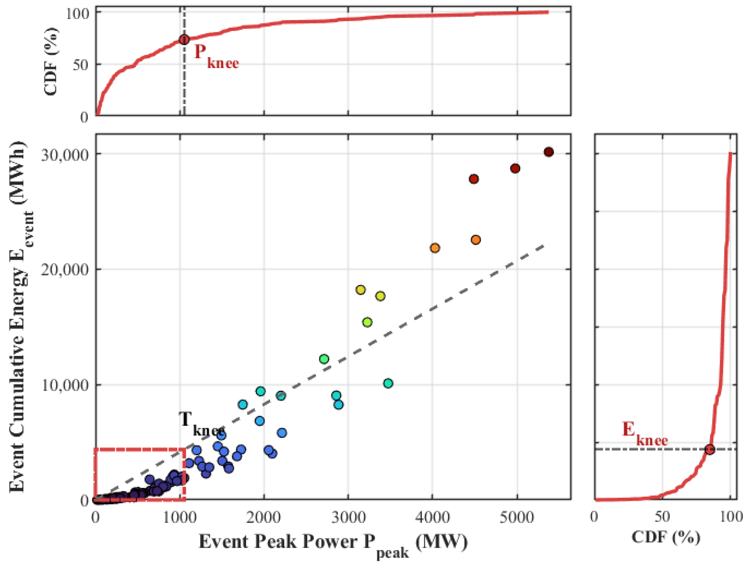
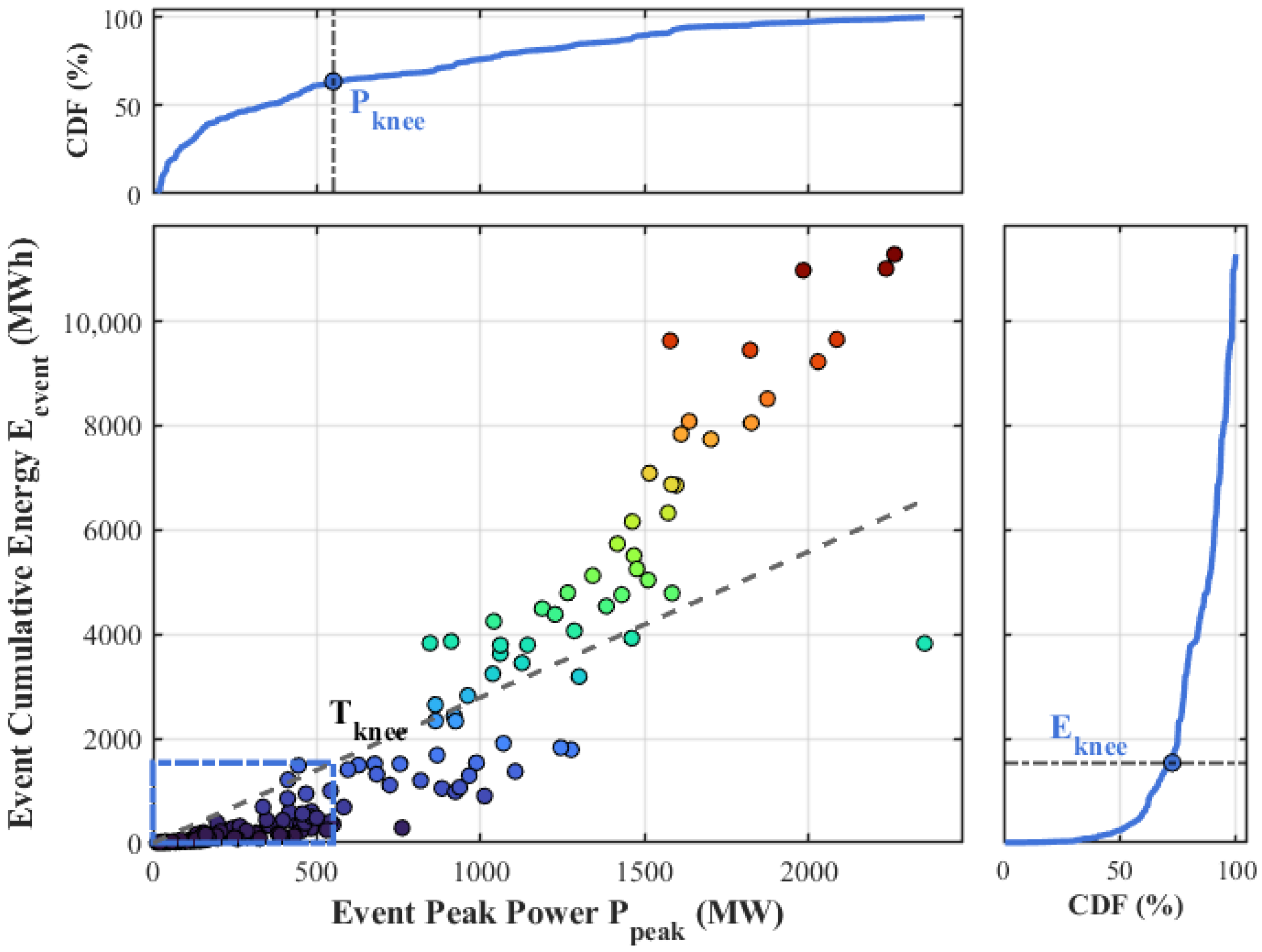
The independent evaluation models for power deficit and curtailment events are illustrated in Figure 10 and Figure 11, respectively.

In the Figure, the color gradient of the scatter points maps to the magnitude of the event cumulative energy E_event, transitioning from cool tones (blue) for low-energy normal events to warm tones (red) for high-energy extreme events.

As shown in Figure 10 and Figure 11, the knee-points $\left(P_{\mathit{knee}}^{\mathit{def}},E_{\mathit{knee}}^{\mathit{def}}\right)$ and $\left(P_{\mathit{knee}}^{\mathit{cur}},E_{\mathit{knee}}^{\mathit{cur}}\right)$ derived from the algorithm respectively lock the critical values between the high-benefit normal operating regions and the extreme event tail-ends for the two types of events. The final system energy storage capacity boundaries (P_knee,E_knee) are determined by taking the maximum of these two values:

$$P_{\mathit{knee}}=\max (P_{\mathit{knee}}^{\mathit{def}},P_{\mathit{knee}}^{\mathit{cur}})$$

(25)

$$E_{\mathit{knee}}=\max (E_{\mathit{knee}}^{\mathit{def}},E_{\mathit{knee}}^{\mathit{cur}})$$

(26)

To assess the stability of the physical knee-points identified by the Kneedle algorithm, this paper conducts a Monte Carlo-based sensitivity analysis. By injecting ±5% Gaussian white noise into the original peak power and cumulative energy sequences to simulate slight fluctuations and measurement uncertainties, 1000 iterative solutions were executed. The statistical results indicate that the coefficients of variation (CV) for P_knee and E_knee are 18.54% and 4.13%, respectively. Although P_knee exhibits a certain degree of fluctuation, it remains constrained within a stable magnitude interval under minor perturbations. This sensitivity analysis confirms that the knee-points captured by the Kneedle algorithm are not numerical couplings overfitted to local data points, but rather stable metrics representing the inherent distribution of system flexibility requirements, thereby providing a robust physical feasible domain for subsequent economic optimization.

After determining the capacity boundaries using the Kneedle algorithm, these boundaries are imposed as feasible domain constraints. A global economic optimization model considering power-energy decoupling is then established by incorporating the system’s annualized total cost objective function. Let P be the rated power and E be the rated capacity of the energy storage system. The annualized total cost C_total(P,E) consists of the annualized equipment investment cost and the remaining penalty losses from uncovered deficits. The two-dimensional comprehensive economic optimization model within the feasible domain [0,P_knee] × [0,E_knee] is expressed as:

$$\begin{array}{l}\underset{P\le P_{\mathit{knee}},E\le E_{\mathit{knee}}}{\min }{C}_{\mathit{total}}(P,E)=\\ F\cdot (c_{p}P+c_{e}E)+\left[r_{\mathit{def}}{\displaystyle \sum _{i=1}^{M_{\mathit{def}}}{E}_{\mathit{unserved},i}^{\mathit{def}}(P,E)+r_{\mathit{cur}}{\displaystyle \sum _{j=1}^{M_{\mathit{cur}}}{E}_{\mathit{unserved},j}^{\mathit{cur}}(P,E)}}\right]\end{array}$$

(27)

where F is the annualized conversion factor; c_p and c_e denote the unit cost of power and energy for energy storage, respectively; r_def and r_cur are the penalty prices for power deficits and curtailment, respectively; $E_{\mathit{unserved},i}^{\mathit{def}}(P,E)$ and $E_{\mathit{unserved},j}^{\mathit{cur}}(P,E)$ represent the residual energy of the i-th deficit event and the j-th curtailment event, respectively, that remains unmitigated after being balanced by the energy storage system under the configuration parameters (P,E).

The optimization problem is numerically solved using MATLAB software (MATLAB R2024 b). The feasible domain [0,P_knee] × [0,E_knee] is discretized into a uniformly spaced 50 × 50 mesh grid. For each discrete grid cell (P,E), the unserved energy $E_{\mathit{unserved},i}^{\mathit{def}}(P,E)$ and $E_{\mathit{unserved},j}^{\mathit{cur}}(P,E)$ are computed by simulating the physical energy shifting process governed by the power and capacity constraints. The specific computational logic inside each cell is as follows: the instantaneous gap power is first clipped by the configured rated power P, and then the cumulative integral of this clipped power within a single independent event is capped by the configured energy capacity E.

By performing a grid search over the two-dimensional grid (P × E), the algorithm automatically solves for the global economic optimal solution (P^*,E^*), that minimizes the system’s annualized total cost, and the optimal charge/discharge duration is subsequently determined as T^* = E^*/P^*. For extreme deficits that exceed this decision boundary, they are designated as intervention intervals for external flexibility resources, to be addressed collaboratively through demand-side response and deep peak-shaving of thermal power units.

5. Case Study

5.1. Basic Data and Parameter Settings

To validate the effectiveness and economic superiority of the proposed optimal energy storage capacity sizing method in a real-world power grid environment, this chapter conducts an assessment based on the operational data of a provincial power grid in northern China, encompassing the entire year with a 15-min resolution (a total of 35,040 time nodes).

The power structure and operational parameters of the case study system are set as follows: the rated capacity of conventional thermal power units is set to P_rate = 660 MW, the minimum technical output ratio is α = 0.50, the downward spinning reserve rate is β = 0.05, and the rapid AGC regulation proportion is γ = 0.05. For the energy storage system, the unit energy cost is c_e = 1000 RMB/kWh (equivalent to 1 million RMB/MWh), the unit power cost is c_p = 400 RMB/kW (equivalent to 0.4 million RMB/MW), and the annualized conversion factor for a 10-year operating cycle is F = 0.12. Regarding grid operational assessment and reliability parameters, the penalty price for power deficit is r_def = 2000 RMB/MWh, and the penalty price for wind and solar curtailment is r_cur = 400 RMB/MWh.

To objectively quantify the performance of the proposed method, following the standard evaluation paradigms in the field of power system planning, three sets of comparative case studies are established:

Case 1: Traditional empirical fixed-duration sizing scheme. Adopting the standardized parameter configuration mode common in commercial energy storage, where the charge/discharge duration is pre-fixed at 4 h, and conventional one-dimensional economic optimization is performed under this constraint.

Case 2: The proposed scheme based on power-energy characteristics of power curtailment and deficit. After solving for the capacity boundaries using the Kneedle algorithm, global total cost synergistic optimization is conducted within this feasible domain.

Case 3: Full physical cumulative balance limit scheme. Aiming at achieving 100% physical zero-deficit and zero-load shedding across the entire grid, full-capacity sizing is carried out based on the extreme peak power and extreme cumulative energy of the largest single event throughout the full cycle.

5.2. Comparison of Energy Storage Sizing Results

The case study data were substituted into the three aforementioned models for calculation, and the key techno-economic indicators for each scheme over the full cycle are presented in

Table 1. Comparison of key techno-economic indicators.

Evaluation Metrics	Case 1	Case 2	Case 3
Rated Power P* (MW)	148.48	357.17	5378.33
Energy Capacity E* (MWh)	593.94	709.69	30,150.13
System Duration T* (h)	4.00	1.99	5.61
Annualized Investment Cost Cinv (106 RMB/year)	78.40	102.30	3876.17
Penalty Loss Cgap (106 RMB/year)	756.94	723.10	0.00
Annualized Total Cost Ctotal (106 RMB/year)	835.34	825.40	3876.17
Complete Event Mitigation Rate (%)	32.57%	49.01%	100.0%

.

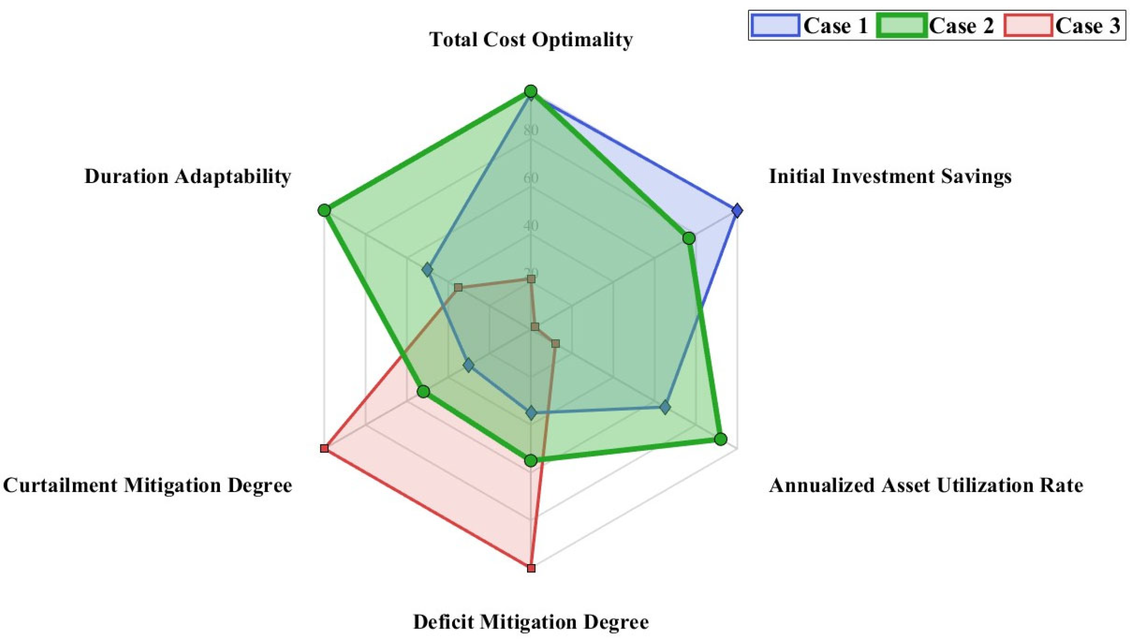
A standardized techno-economic evaluation matrix covering six dimensions—total cost optimality, initial investment savings, annualized asset utilization rate, deficit mitigation degree, curtailment mitigation degree, and duration adaptability—was constructed, and the multi-dimensional radar chart shown in Figure 12 was plotted.

Combining the data in Table 1 with the characteristics of the radar chart in Figure 12, the following conclusions can be drawn:

Case 1 (Traditional 4 h fixed-duration scheme): The rated power is locked at 148.48 MW. When faced with high-frequency, high-power pulse shocks, the system experiences power clipping by the converter, resulting in a complete mitigation rate for curtailment and deficit events of only 32.57%, which triggers massive penalty losses of 756.94 million RMB/year. The blue polygon in the radar chart exhibits a limited overall morphology, indicating that rigidly binding the charge/discharge duration without considering actual gap characteristics induces structural mismatches characterized by either power redundancy or insufficiency.

Case 3 (Full physical limit scheme): Although Case 3 achieves 100% physical safety, it is forced to configure an excessive capacity of 5378.33 MW and 30,150.13 MWh to mitigate extreme events with an occurrence probability of less than 1%, leading to a total investment scale exceeding 380 million RMB. In the radar chart, the red polygon presents an extremely distorted, unilateral extension shape; while it maximizes the security assurance dimension, it shrinks toward the origin in terms of investment savings, total cost, and asset utilization rate.

Case 2 (The proposed scheme): By employing two-dimensional decoupling, the proposed scheme adaptively identifies the optimal system duration of 1.99 h for normal net load fluctuations. With a marginal increase in annualized equipment investment of approximately 23.9 million RMB, the rated power is appropriately released to 357.17 MW, causing the complete mitigation rate for curtailment and deficit events to jump from 32.57% to 49.01%, an increase of 16.44 percentage points. Simultaneously, as penalty losses are significantly reduced by 33.84 million RMB/year, the annualized total system cost converges to 825.40 million RMB/year, demonstrating absolute superiority in both total cost economy and unit investment efficiency.

5.3. Comparative Analysis Under Future Scenarios with Increased Renewable Energy Penetration

To verify the forward-looking adaptability and scenario robustness of the proposed optimal energy storage capacity sizing method in the long-term evolution of future novel power systems, this section constructs evolutionary scenarios with an increasing scale of installed renewable energy. By proportionally scaling the wind and photovoltaic (PV) output data, the cost sensitivity and growth elasticity of each scheme during the penetration growth process are compared.

Taking the provincial wind and solar power output data as the baseline and keeping the grid power load level unchanged, a renewable energy installed capacity multiplication factor, κ, is introduced to construct a three-level evolutionary tier with penetration rate increments of 20% (κ = 1.20), 25% (κ = 1.25), and 30% (κ = 1.30). The chronological net load evolution equation under each scenario is expressed as:

$$L_{\mathit{net}}^{(\kappa )}(t)=L(t)-\kappa \cdot (W(t)+S(t))$$

(28)

With the increment of κ, the severe depression of the net load caused by massive midday PV generation and the steep ramping during evening sunset are non-linearly amplified, imposing more stringent support requirements on the energy storage system. By substituting the data of different penetration rates into the three schemes for independent solutions, the comparison of the economic costs and event mitigation rates of the energy storage configurations under various scenarios is shown in

Table 2. Comparison table of energy storage sizing schemes under different renewable energy penetration scenarios.

Penetration Scenario	Scheme	Rated Power (MW)	Energy Capacity (MWh)	System Duration (h)	Annualized Total Cost (106 RMB/year)	Complete Event Mitigation Rate (%)
+20%	Case1	917.95	3671.79	4.00	1538.43	64.71%
	Case2	1169.40	3368.76	2.88	1520.16	71.01%
	Case3	6198.65	38,208.11	6.16	4882.50	100.00%
+25%	Case1	1141.03	4564.10	4.00	1748.68	69.86%
	Case2	1344.84	4155.28	3.09	1741.46	73.05%
	Case3	6833.12	43,986.24	6.44	5606.64	100.00%
+30%	Case1	1289.74	5158.97	4.00	1939.63	69.90%
	Case2	1505.78	5012.29	3.33	1936.28	74.56%
	Case3	7467.58	50,036.69	6.70	6365.09	100.00%

.

Observing the comparison results in Table 2, it is evident that across all projected future high-penetration scenarios, the annualized total system cost of the proposed scheme consistently remains the global minimum. Meanwhile, as the penetration rate continues to climb, the annualized total cost of Case 1 exhibits a continuous upward trend, yet its complete mitigation rate of curtailment and deficit events falls into a distinct growth stagnation, merely moving from 69.86% in the +25% scenario to 69.90% in the +30% scenario. The proposed scheme accurately captures the variation laws of the grid net load curve caused by the future large-scale PV integration, and the calculated optimal charge/discharge duration T^* steadily climbs from 2.88 h to 3.09 h and 3.33 h. In terms of mitigation efficacy, the event mitigation rate also steadily increases from 71.01% to 74.56%, gradually widening the gap with Case 1. This proves that the proposed energy storage capacity optimal sizing method, which matches the power-energy characteristics, possesses the most robust long-term planning guiding value in future novel power systems with continuously increasing renewable energy grid integration.

6. Conclusions

To address the coexistence of power curtailment and deficit induced by net load fluctuations in power grids with a high proportion of renewable energy, this paper proposes a methodological framework for optimal energy storage capacity sizing. This framework encompasses the determination of conventional thermal power committed capacity, the quantification of curtailment and deficit events, the solution of physical saturation knee-points, and economic synergistic optimization. The main contributions and findings of this paper are summarized as follows:

• Deepening traditional daily macro-aggregation into a quantitative model of independent physical events. This method authentically restores the short-term power shocks and long-term energy accumulation experienced by the power grid, proving the feasibility of decoupling and independently optimizing the power and capacity of energy storage.
• Establishing a boundary demarcation mechanism for energy storage capacity based on the Kneedle algorithm. Serving as the upper limit for energy storage configuration, it provides a rigorous feasible domain constraint for subsequent economic optimization, effectively avoiding long-term equipment idling and capital wastage.
• A case study of a provincial power grid in northern China demonstrates that the proposed method significantly enhances the complete mitigation rate of curtailment and deficit events while achieving the lowest global annualized total system cost. This provides a rigorous quantitative decision-making basis for energy storage planning and multi-resource collaborative intervention in power grids with high renewable penetration.

Furthermore, this paper focuses on the extraction of physical boundaries and macro-economic optimization during the energy storage sizing phase. The curtailment and deficit processes are abstracted as independent physical events for decoupled evaluation. A full-cycle chronological operational simulation model—incorporating charge/discharge efficiencies, self-discharge losses, and continuous State of Charge (SOC) constraints—has not yet been established. Under extreme weather conditions, if the system lacks sufficient charging recovery windows, the actual mitigation effectiveness might slightly deviate. Therefore, validating the optimal sizing scheme derived in this study through a full-chronological production simulation model with refined equipment operational constraints will be a key focus of our future work.

References

1. Cui, Y.; Zhang, H.Q.; Zhong, W.Z.; Zhao, Y.; Zhang, J.; Wang, M. Multi-source Optimal Scheduling of Renewable Energy High-permeability Power System with CSP Plants Considering Demand Response. High Volt. Eng. 2020, 46, 1486–1496. [Google Scholar] [CrossRef]
2. Bi, P.P.; Xu, X.Y.; Mei, W.M.; Zhang, L.; Li, M.; Bai, B. Study on Cascaded Tripping-off Risk Assessment Method and Delivery Capacity of Wind Power Base. Power Syst. Technol. 2019, 43, 903–910. [Google Scholar] [CrossRef]
3. Hou, Q.C.; Zhang, N.; Du, E.; Miao, M.; Peng, F.; Kang, C. Probabilistic duck curve in high PV penetration power system: Concept, modeling, and empirical analysis in China. Appl. Energy 2019, 242, 205–215. [Google Scholar] [CrossRef] [Scilit]
4. Calero, I.; Cañizares, C.A.; Bhattacharya, K.; Baldick, R. Duck curve mitigation in power grids with high penetration of PV generation. IEEE Trans. Smart Grid 2022, 13, 314–329. [Google Scholar] [CrossRef] [Scilit]
5. Deng, T.T.; Lou, S.H.; Tian, X.; Wu, Y.; Li, N. Optimal Dispatch of Power System Integrated with Wind Power Considering Demand Response and Deep Peak Regulation of Thermal Power Units. Autom. Electr. Power Syst. 2019, 43, 34–41. [Google Scholar]
6. Li, J.H.; Zhang, J.H.; Mu, G.; Gu, Y.; Yan, G.; Shi, S. Hierarchical Optimization Scheduling of Deep Peak Shaving for Energy-storage Auxiliary Thermal Power Generating Units. Power Syst. Technol. 2019, 43, 3961–3970. [Google Scholar] [CrossRef]
7. Xu, G.D.; Cheng, H.Z.; Ma, Z.F.; Fan, S.; Fang, S.; Ma, Z. Overview of ESS planning methods for alleviating peak-shaving pressure of grid. Electr. Power Autom. Equip. 2017, 37, 3–11. [Google Scholar] [CrossRef]
8. Aneke, M.; Wang, M. Energy storage technologies and real life applications—A state of the art review. Appl. Energy 2016, 179, 350–377. [Google Scholar] [CrossRef] [Scilit]
9. Denholm, P.; Jorgenson, J.; Jenkin, T.; Hummon, M.; Palchak, D.; Kirby, B.; Ma, O.; O′MAlley, M. The Value of Energy Storage for Grid Applications; NREL/TP-6A20-58465; NREL National Renewable Energy Laboratory: Golden, CO, USA, 2013. [Google Scholar] [CrossRef] [Scilit]
10. Bahramirad, S.; Reder, W.; Khodaei, A. Reliability-constrained optimal sizing of energy storage system in a microgrid. IEEE Trans. Smart Grid 2012, 3, 2056–2062. [Google Scholar] [CrossRef] [Scilit]
11. Liu, R.H.; Jia, Y.B.; Fu, K.N.; Han, X.Q. Double-layer Optimization for Wind and Energy Storage Capacity Configuration in Transmission Network Considering Security Reserve Constraints. Power Syst. Technol. 2021, 45, 2741–2752. [Google Scholar] [CrossRef]
12. Yan, G.G.; Feng, X.D.; Li, J.H.; Mu, G.; Xie, G.; Dong, X.; Wang, Z.; Yang, K. Optimization of Energy Storage System Capacity for Relaxing Peak Load Regulation Bottlenecks. Proc. CSEE 2012, 32, 27–35+22. [Google Scholar] [CrossRef]
13. Sun, Y.S.; Tang, X.S.; Sun, X.Z.; Jia, D.; Zhang, G.; Wang, P. Research on Energy Storage Capacity Allocation Method for Smoothing Wind Power Fluctuations. Proc. CSEE 2017, 37, 88–97. [Google Scholar] [CrossRef]
14. Babacan, O.; Torre, W.; Kleissl, J. Siting and sizing of distributed energy storage to mitigate voltage impact by solar PV in distribution systems. Sol. Energy 2017, 146, 199–208. [Google Scholar] [CrossRef] [Scilit]
15. Zhang, Y.; Dong, Z.Y.; Luo, F.; Zheng, Y.; Meng, K.; Wong, K.P. Optimal allocation of battery energy storage systems in distribution networks with high wind power penetration. IET Renew. Power Gener. 2016, 10, 1105–1113. [Google Scholar] [CrossRef] [Scilit]
16. Liu, J.C.; Chen, X.; Xiang, Y. Optimal Sizing and Investment Benefit Analysis for Energy Storage of Electricity Retailers Under Market Mechanisms Considering Shared Mode. Power Syst. Technol. 2020, 44, 1740–1750. [Google Scholar] [CrossRef]
17. Yang, L.B.; Cao, Y.; Wei, W.; Chen, L.; Mei, S. Configuration Method of Energy Storage for Wind Farms Considering Wind Power Uncertainty and Wind Curtailment Constraint. Autom. Electr. Power Syst. 2020, 44, 45–52. [Google Scholar]
18. Han, X.N.; Li, J.M.; Wen, J.Y.; Ai, X.; Li, J.; Luo, W. Optimization for Robust Energy Storage Allocation in Power System With Multiple Wind Farms Integrated. Proc. CSEE 2015, 35, 2120–2127. [Google Scholar] [CrossRef]
19. Zhu, J.Y.; Liu, Y.; Xu, L.X.; Jiang, Z.; Lin, X. Adjustable Robust Optimization for Energy Storage System in Distribution Network Based on Wind Power Full Accommodation. Power Syst. Technol. 2018, 42, 1875–1883. [Google Scholar] [CrossRef]
20. Qian, W.T.; Zhao, C.F.; Wan, C.; Huang, Y.; Zhu, B.; Chen, W. Probabilistic Forecasting Based Stochastic Optimal Dispatch and Control Method of Hybrid Energy Storage for Smoothing Wind Power Fluctuations. Proc. CSEE 2021, 45, 18–27. [Google Scholar]
21. Sun, W.Q.; Song, H.; Qin, Y.H.; Li, H. Energy Storage System Optimal Allocation Considering Flexibility Supply and Demand Uncertainty. Power Syst. Technol. 2020, 44, 4486–4497. [Google Scholar] [CrossRef]
22. Baker, K.; Hug, G.; Li, X. Energy storage sizing taking into account forecast uncertainties and receding horizon operation. IEEE Trans. Sustain. Energy 2017, 8, 331–340. [Google Scholar] [CrossRef] [Scilit]
23. Li, J.; Xu, Z.; Liu, H.; Wang, C.; Wang, L.; Gu, C. A Wasserstein distributionally robust planning model for renewable sources and energy storage systems under multiple uncertainties. IEEE Trans. Sustain. Energy 2023, 14, 1346–1356. [Google Scholar] [CrossRef] [Scilit]
24. Alharbi, H.; Bhattacharya, K. Stochastic optimal planning of battery energy storage systems for isolated microgrids. IEEE Trans. Sustain. Energy 2018, 9, 211–227. [Google Scholar] [CrossRef] [Scilit]
25. Cui, Y.; Zhou, H.J.; Zhong, W.Z.; Hui, X.; Zhao, Y. Two-stage Day-ahead and Intra-day Rolling Optimization Scheduling Considering Joint Peak Regulation of Generalized Energy Storage and Thermal Power. Power Syst. Technol. 2021, 45, 10–20. [Google Scholar] [CrossRef]
26. Jin, L.; Fang, X.Y.; Cai, Z.H.; Chen, D.; Li, Y. Multiple Time-scales Source-storage-load Coordination Scheduling Strategy of Grid Connected to Energy Storage Power Station Considering Characteristic Distribution. Power Syst. Technol. 2020, 44, 3641–3650. [Google Scholar] [CrossRef]
27. Li, Z.A.; Chen, L.J.; Liu, D.W.; Chen, F.; Zheng, T.; Mei, S. Subsidy Pricing Method for Stackelberg-game-based Energy Storage System. High Volt. Eng. 2020, 46, 519–526. [Google Scholar] [CrossRef]
28. Zhu, D.W.; Zhang, Y.J.A. Optimal coordinated control of multiple battery energy storage systems for primary frequency regulation. IEEE Trans. Power Syst. 2019, 34, 555–565. [Google Scholar] [CrossRef] [Scilit]
29. Nosair, H.; Bouffard, F. Flexibility envelopes for power system operational planning. IEEE Trans. Sustain. Energy 2015, 6, 800–809. [Google Scholar] [CrossRef] [Scilit]
30. Li, H.; Zhang, N.; Bao, W.; Fan, Y.; Dong, L.; Cai, P. Modeling and planning of multi-timescale flexible resources in power systems. CSEE J. Power Energy Syst. 2024, 11, 1533–1543. [Google Scholar] [CrossRef] [Scilit]
31. Yang, P.; Nehorai, A. Joint optimization of hybrid energy storage and generation capacity with renewable energy. IEEE Trans. Smart Grid 2014, 5, 1566–1574. [Google Scholar] [CrossRef] [Scilit]
32. Satopaa, V.; Albrecht, J.; Irwin, D.; Raghavan, B. Finding a “Kneedle” in a haystack: Detecting knee points in system behavior. In Proceedings of the 31st International Conference on Distributed Computing Systems Workshops, Minneapolis, MN, USA, 20–24 June 2011; IEEE: New York, NY, USA, 2011; pp. 166–171. [Google Scholar] [CrossRef] [Scilit]
Figure 1. (a) Original load curve. (b) Wind and PV output curve. (c) Net load curve.
Energies 19 04637 g001
Figure 2. Schematic of thermal power regulation capacity.
Energies 19 04637 g002
Figure 3. Schematic diagram of temporal states.
Energies 19 04637 g003
Figure 4. Schematic diagram of deficit area.
Energies 19 04637 g004
Figure 5. Schematic diagram of curtailment area.
Energies 19 04637 g005
Figure 6. Temporal distribution of curtailment and deficit events.
Energies 19 04637 g006
Figure 7. Sorted duration curve of curtailment and deficit events.
Energies 19 04637 g007
Figure 8. Illustration of energy storage envelope coverage.
Energies 19 04637 g008
Figure 9. (a) Evolution curve of economic characteristics under capacity under-sizing. (b) Evolution curve of economic characteristics under capacity over-sizing.
Energies 19 04637 g009
Figure 10. Knee-point sizing evaluation plot for deficit events.
Energies 19 04637 g010
Figure 11. Knee-point sizing evaluation plot for curtailment events.
Energies 19 04637 g011
Figure 12. Radar chart of comprehensive techno-economic performance.
Energies 19 04637 g012