Regional Role Matching and Energy Temporal Coupling-Based Coordinated Dispatch of Multiple Pumped Storage Plants Under Zonal Transmission Constraints

Abstract

Although large-scale wind and solar power provide green electricity, their intermittency and reverse-peak characteristics pose severe challenges to the secure operation of power systems. Pumped storage hydropower (PSH), as the most mature and economically attractive large-scale energy storage technology, enables temporal energy shifting and serves as a core flexible resource for smoothing renewable fluctuations and peak load shaving. In a new power system dominated by renewables, the reverse distribution between resources and loads gives rise to a typical “three-zone coexistence” pattern, i.e., renewable-rich zones, load centers, and hub zones coexist. However, existing research lacks in-depth modeling of zonal functional differences and fails to reveal the coupling mechanism between inter-zonal section constraints and the temporal energy behavior of pumped storage plants (PSPs). To address these gaps, this paper proposes a zonal-differentiated optimal dispatch model for multiple PSPs considering inter-zonal section constraints. The model establishes a “zonal role–PSP behavior” matching mechanism, assigning differentiated objectives and operational constraints to PSPs located in different zones, and thereby automatically generating charging/discharging strategies that match each zone’s functional positioning. It integrates section power flow constraints with the energy balance equations of PSPs in each zone into a unified framework, quantifying how section congestion restricts the “cross-zone energy shifting” efficiency of PSPs. Furthermore, a congestion-driven adaptive rule is derived from the above coupling framework. Case studies on a three-zone test system demonstrate that the proposed model effectively reduces wind and solar curtailment, alleviates section overloading, and lowers total operating costs, while the adaptive rule provides real-time decision support for dispatchers. The proposed model is applicable to power grids at various levels exhibiting the “three-zone coexistence” characteristic, offering theoretical support and a practical tool for the joint dispatch of multiple PSPs under high-penetration renewable energy integration.

1. Introduction

Building a new power system dominated by renewable energy is a key pathway to achieving “carbon peak and carbon neutrality” goals [1,2,3]. While large-scale integration of wind and solar power provides green electricity, its intermittency and reverse peak characteristics bring severe challenges to the secure and economic operation of power systems [4,5,6]. Pumped storage hydropower (PSH), as the most mature and economically attractive large scale energy storage technology [7], enables temporal energy shifting and is a core flexible resource for smoothing renewable fluctuations and peak load shaving [8,9,10]. Pumped storage hydropower can be divided into two categories: pure pumped storage and hybrid pumped storage. The former has both upper and lower reservoirs artificially constructed with water circulated between them, while the latter is retrofitted from conventional hydropower stations and requires comprehensive consideration of reservoir operation in its scheduling [11].

In new power systems, the reverse distribution between resources and loads gives rise to a typical “three-zone coexistence” pattern, where renewable-rich zones, load centers, and interconnection hubs coexist within the same power grid [12]. Taking China, which has the world’s largest installed capacity of wind and solar power, as an example: at the national level, the distribution of wind and solar resources is inversely related to load centers—the renewable-rich areas in Northwest and North China experience high output fluctuations and limited local consumption [13]; the eastern load centers face a continuously widening power deficit; and the central hub grids serve as transfer nodes for inter-regional power re-dispatch [14]. Similarly, within China’s regional power grids (e.g., Northwest, Central, and East China Grids) and provincial grids, there are also concurrent zones of renewable-rich areas, load centers, and interconnection hubs [15,16]. This spatial characteristic provides the practical foundation for regional role matching in the dispatch of pumped storage plants: pumped storage in different zones assumes corresponding regulation roles based on its location and grid function. Meanwhile, by virtue of their energy storage capability, pumped storage plants (PSPs) can transfer and regulate electric energy across different time scales, forming an operational mechanism of energy temporal coupling [6,7,8]. When integrating these two aspects from a spatio-temporal perspective, not only can the coordinated dispatch of multiple pumped storage plants under zonal transmission constraints fully leverage the spatial coordination advantage of regional role matching and the time-shifting capability of energy temporal coupling, but it is also of great significance for the spatio-temporally coordinated dispatch of high-penetration renewable energy power systems and the joint optimization of multiple pumped storage plants.

To date, the vast majority of studies have focused on the feasibility analysis of pumped storage as a technical pathway [17,18,19,20]. For instance, a comparison between battery and pumped storage for seawater desalination systems shows that battery storage achieves a lower levelized cost of water, while pumped storage, although slightly more expensive, significantly reduces carbon emissions [17]. A dispatch model coupling pumped storage with wind–solar power for green hydrogen production demonstrates that pumped storage can effectively increase hydrogen production profit and its own utilization through electricity price arbitrage [18]. For rural electrification scenarios, a comparison of different photovoltaic technologies combined with pumped storage and battery storage reveals that the configuration of polycrystalline silicon PV, hydropower, and pumped storage is the most economical and efficient solution for achieving 100% renewable energy [19]. Furthermore, a study on the joint operation of a pumped storage plant with other power plants finds that, under wind and solar power uncertainty, the pumped storage plant can maximize the total system profit [20].

Some scholars have focused on the single-zone joint optimization of pumped storage plants and renewable energy. “Energy-power” dual variables were introduced for PSPs, and charging/discharging strategies were solved via mixed-integer nonlinear programming, effectively improving renewable integration [21]. Nevertheless, these single-zone models ignore the physical limits of inter-zonal power exchange and are not directly applicable to multi-zone interconnected systems. In recent years, multi-zone coordinated dispatch has become a research hotspot. Numerous studies have shown that transmission section constraints, line capacities, and security constraints are key factors affecting the operational benefits of pumped storage hydropower plants. The issue of transmission channel capacities severely restricting renewable energy accommodation is addressed using multistage partitioned section chance constraints and hydropower compensation for uncertainty, effectively alleviating congestion and reducing curtailment [22]. This demonstrates that section constraints directly determine cross-regional power transfer capability; ignoring them leads to physically infeasible dispatch schedules. A linearized simplified network-constrained unit commitment model is proposed for long-term planning, combining a dispatch-only model with a clustered unit commitment model via linking constraints [23]. It emphasizes that line capacity constraints significantly alter the output allocation of different power sources, and neglecting them overestimates the system’s flexible regulation capability. A novel iterative constraint-screening method that eliminates 99.4% of transmission constraints is proposed to tackle the computational bottleneck in security-constrained unit commitment [24]. The study points out that only a small subset of critical line constraints is active in actual operation, yet these active constraints are crucial for determining the charging/discharging timing and power levels of flexible resources such as pumped storage. In summary, transmission section constraints, line capacities, and security constraints together constitute the physical boundary for pumped storage plants to perform their spatio-temporal energy shifting function. Accurately modeling these constraints is a prerequisite for realizing the regulation benefits of pumped storage and ensuring secure grid operation.

Thus, the existing literature lacks an in-depth PSP dispatch modeling of zonal functional differences. In a renewable-rich zone, PSPs primarily solve local curtailment and shift surplus energy for later export; in a load center, they mainly relieve evening peak pressure; in a hub zone, they flexibly coordinate power flows in multiple directions. However, current models assign identical objective weights and constraint forms to all PSPs, and therefore cannot automatically generate charging/discharging patterns that match distinct zonal roles. More importantly, when section congestion occurs, the adaptive strategies of PSPs in different zones—e.g., reducing pumping in the sending zone or increasing generation in the receiving zone—have not been systematically studied. Given the research gaps described above, the following core issues remain unaddressed:

• The functional roles of zones (renewable-rich, load center, hub) are not mapped into distinct operation modes of PSPs, so the model cannot actively generate strategies that match each zone’s positioning.
• The coupling mechanism between section constraints and the temporal energy behavior of PSPs remains unrevealed. How section congestion forces PSPs to adjust their inter-temporal energy shift plans lacks a quantitative model.
• There is no adaptive rule for PSP charging/discharging that responds to section congestion, making it difficult for dispatch schedules to remain both economic and reliable when sections become tight.

To address the above gaps, this paper proposes a coordinated dispatch model for multiple PSPs under zonal section constraints, with the following main contributions.

(i)

A “zonal role–PSP behavior” matching mechanism is established. Based on zonal functional attributes, PSPs located in different zones are assigned differentiated characteristics: in a renewable-rich zone, priority is given to pumping during renewable surplus periods and generating for export during off-peak hours or when sections permit (encouraging “low-price storage and delayed export” through low opportunity costs); in a load center, priority is given to generation during evening peaks; in a hub zone, the model allows both pumping using power from the renewable-rich zone and discharging to the load center, using bidirectional power variables to achieve “energy interchange.” Through this differentiated modeling, the optimization automatically generates charging/discharging patterns that match each zone’s role.

(ii)

A coordination framework coupling inter-zonal sections and PSP energy balance is developed. The energy balance equations of PSPs in each node and the power flow constraints of inter-zonal sections are unified into a single optimization model. This framework quantifies for the first time how section congestion restricts the “cross-zone energy shifting” efficiency of PSPs, and provides guidance information for section capacity expansion or PSP capacity addition.

(iii)

Based on the above framework, an intuitive congestion-response rule is derived. If the sending-zone → receiving-zone section is saturated, the sending-zone PSP should maintain or increase pumping (to absorb surplus local power and reduce export demand), or if generating, switch to pumping; the receiving-zone PSP should stop pumping using imported power and switch to local generation. If the reverse direction is saturated, the original receiving-zone PSP should maintain or increase pumping, or if generating, switch to pumping; the original sending-zone PSP should stop pumping using imported power, or if pumping, switch to generation. This rule can be directly embedded into a decision support system, providing operators with clear operational guidelines.

The remainder of this paper is organized as follows. Section 2 presents the mathematical model. Section 3 gives the congestion-response PSP rule. Section 4 describes case studies and results. Section 5 provides sensitivity analysis. Section 6 concludes the paper and outlines future research directions.

2. Coordinated Dispatch Modeling of Multiple PSPs Considering Zonal Differences

2.1. Objective Function with Zonal Differentiation

To explicitly represent the distinct operational roles of different zones (e.g., renewable-rich zone, load center, hub zone), the objective function is formulated with a zonal index $z\in Z$. This allows for assigning zone-specific cost coefficients to thermal units, PSPs, wind, and solar generation, thereby reflecting the different economic priorities of each zone—for instance, lower pumping cost in a renewable-rich zone to encourage storage of surplus energy, and higher generation value in a load center to meet peak demand.

The modified objective function is given in (1):

$$\begin{array}{cc} & \mathrm{m}\mathrm{i}\mathrm{n}{\displaystyle \sum _{t=1}^T}[\Delta t{\displaystyle \sum _{z\in Z}}{\displaystyle \sum _{g\in G_z^{\mathrm{th}}}}{c}_{g,z}^{\mathrm{fuel}}{p}_{g,z,t}+{\displaystyle \sum _{z\in Z}}{\displaystyle \sum _{g\in G_z^{\mathrm{th}}}}\left(c_{g,z}^{\mathrm{su}}{v}_{g,z,t}+c_{g,z}^{\mathrm{sd}}{w}_{g,z,t}\right)\\ & +\Delta t{\displaystyle \sum _{z\in Z}}{\displaystyle \sum _{j\in G_z^{\mathrm{pump}}}}\left(c_{j,z}^{\mathrm{pump}}{p}_{j,z,t}^{\mathrm{pump}}+c_{j,z}^{\mathrm{gen}}{p}_{j,z,t}^{\mathrm{gen}}\right)\\ & +\Delta t{\displaystyle \sum _{z\in Z}}{\displaystyle \sum _{w\in G_z^{\mathrm{wind}}}}{c}_{w,z}^{\mathrm{wind}}{p}_{w,z,t}^{\mathrm{wind}}+\Delta t{\displaystyle \sum _{z\in Z}}{\displaystyle \sum _{s\in G_z^{\mathrm{solar}}}}{c}_{s,z}^{\mathrm{solar}}{p}_{s,z,t}^{\mathrm{solar}}\\ & +\Delta t{\displaystyle \sum _{z\in Z}}{\displaystyle \sum _{n\in N_z}}\left(C^{\mathrm{curtail}}{\mathrm{curt}}_{n,z,t}+C^{\mathrm{ls}}{\mathrm{ls}}_{n,z,t}\right)\end{array}$$

(1)

The first line captures the fuel cost of thermal units (converted from power to energy by $\Delta t$) plus their startup/shutdown costs, all summed over zones. The second line covers PSP pumping and generation costs. The third line includes the variable O&M costs of wind and solar power. The last line imposes high penalties on renewable curtailment and load shedding. By introducing zonal indices, the model can differentiate cost coefficients according to each zone’s functional role, which is essential for implementing the “Regional Role Matching” mechanism.

2.2. Inter-Zonal Constraints

2.2.1. System-Wide Nodal Power Balance

Equation (2) enforces the power balance at each node $n$ in zone $z$ at each time $t$. The left-hand side sums all injections: thermal generation, PSP generation, actual wind and solar outputs, and incoming inter-zonal power flows. The right-hand side sums all withdrawals: PSP pumping, net load (demand minus load shedding), and outgoing inter-zonal flows. Load shedding ${\mathrm{ls}}_{n,z,t}$ is permitted under extreme conditions but is heavily penalized in the objective function to ensure supply reliability.

$$\begin{array}{cc} & {\displaystyle \sum _{g\in G_{n,z}^{\mathrm{th}}}}{p}_{g,z,t}+{\displaystyle \sum _{j\in G_{n,z}^{\mathrm{pump}}}}{p}_{j,z,t}^{\mathrm{gen}}+{\displaystyle \sum _{w\in G_{n,z}^{\mathrm{wind}}}}{p}_{w,z,t}^{\mathrm{wind}}+{\displaystyle \sum _{s\in G_{n,z}^{\mathrm{solar}}}}{p}_{s,z,t}^{\mathrm{solar}}+{\displaystyle \sum _{l\in L_{n,z}^{\mathrm{in}}}}{f}_{l,t}\\ & ={\displaystyle \sum _{j\in G_{n,z}^{\mathrm{pump}}}}{p}_{j,z,t}^{\mathrm{pump}}+D_{n,z,t}-{\mathrm{ls}}_{n,z,t}+{\displaystyle \sum _{l\in L_{n,z}^{\mathrm{out}}}}{f}_{l,t},\forall z,\forall n\in N_z,\forall t\end{array}$$

(2)

2.2.2. Section Capacity Constraints

In practical power systems, inter-zonal power exchange is typically realized through a transmission corridor composed of multiple parallel tie lines, referred to as a section. The transfer capability of this corridor is limited by two types of constraints: (i) the thermal limit of each individual line, determined by conductor cross-section, cooling conditions, etc.; and (ii) the overall stability limit of the entire corridor, e.g., dynamic stability, transient stability, or the power transfer capability under the N 1 criterion. These two limits are not numerically equivalent—the overall stability limit is often smaller than the algebraic sum of the individual thermal limits. Consequently, three modeling options arise when modeling section capacity constraints in dispatch optimization. The modeling options are presented below, which can be selected based on data availability and operational requirements.

Total Section Capacity Only (Option 1): This option treats the section as a single entity and limits only the sum of all tie-line flows, without distinguishing individual lines. It is the most common model and requires minimal data. The total power flow on section $m$ at time $t$, $f_{m,t}$, lies within the maximum total transfer capacity of section m, $F_m^{\mathrm{m}\mathrm{a}\mathrm{x}}$.

$$-F_m^{\mathrm{m}\mathrm{a}\mathrm{x}}\le f_{m,t}\le F_m^{\mathrm{m}\mathrm{a}\mathrm{x}},\forall m,\forall t$$

(3)

where positive values indicate flow from sending to receiving zone; negative values indicate the opposite direction.

Individual Tie-line Capacity Only (Option 2): This option disaggregates the section into individual tie-lines and imposes an independent capacity limit on each line. It is suitable for scenarios where line capacities are independent and not coupled. The total section flow is the sum of individual line flows.

$$-F_l^{\mathrm{m}\mathrm{a}\mathrm{x}}\le f_{l,t}\le F_l^{\mathrm{m}\mathrm{a}\mathrm{x}},\forall m,\forall l\in L_m,\forall t$$

(4)

$$f_{m,t}={\displaystyle \sum _{l\in L_m}}{f}_{l,t}$$

(5)

Here, $L_m$ is the set of tie-lines belonging to section $m$, and $f_{l,t}$ is the power flow on line $l$ at time $t$ from sending node $n_i$ to ending node $n_j$.

Both Individual and Total Section Capacity (Option 3): This option enforces both individual line limits and a total section limit. The total section capacity $F_m^{\mathrm{m}\mathrm{a}\mathrm{x}}$ is typically less than or equal to the sum of individual line capacities ($F_m^{\mathrm{m}\mathrm{a}\mathrm{x}}\le {\sum }_l{F}_l^{\mathrm{m}\mathrm{a}\mathrm{x}}$), reflecting system-wide stability limits. This is the most stringent model for practical grids.

$$-F_l^{\mathrm{m}\mathrm{a}\mathrm{x}}\le f_{l,t}\le F_l^{\mathrm{m}\mathrm{a}\mathrm{x}},\forall m,\forall l\in L_m,\forall t$$

(6)

$$-F_m^{\mathrm{m}\mathrm{a}\mathrm{x}}\le {\displaystyle \sum _{l\in L_m}}{f}_{l,t}\le F_m^{\mathrm{m}\mathrm{a}\mathrm{x}},\forall m,\forall t$$

(7)

The core differences among the three options of section capacity constraints are given below: Option 1 ignores internal flow distribution and concerns only the total power; Option 2 concerns only individual line limits and allows the total section power to reach the sum of the line limits; Option 3 imposes both total and individual limits, making it the most stringent model. The relationships among the three options are given below: Option 2 is the basis of Option 1: If individual line limits are known, a conservative estimate of the total section limit can be obtained as $F_m^{\mathrm{m}\mathrm{a}\mathrm{x}}={\sum }_l{F}_l^{\mathrm{m}\mathrm{a}\mathrm{x}}$. Then, Option 1 becomes a relaxation of Option 2. Option 3 is a combination of Option 1 and Option 2: When $F_m^{\mathrm{m}\mathrm{a}\mathrm{x}}<{\sum }_l{F}_l^{\mathrm{m}\mathrm{a}\mathrm{x}}$, the feasible region of Option 3 is the intersection of the feasible regions of Option 1 and Option 2, and therefore tighter. If the actual overall stability limit happens to equal the sum of the individual line limits, and then Option 3 is equivalent to Option 2, and Option 1 (with that sum) is also equivalent to both.

2.3. Intra-Zonal Constraints

2.3.1. Pumped Storage Plant Constraints

Equation (8) describes the energy balance of the PSP reservoir. Pumping increases stored energy (multiplied by efficiency ${\eta }_j^{\mathrm{pump}}<1$), while generation decreases it (divided by efficiency ${\eta }_j^{\mathrm{gen}}<1$). This constraint embodies the temporal energy coupling of PSPs.

$$E_{j,z,t}=E_{j,z,t-1}+{\eta }_j^{\mathrm{pump}}{p}_{j,z,t}^{\mathrm{pump}}\Delta t-{\displaystyle \frac{p_{j,z,t}^{\mathrm{gen}}\Delta t}{{\eta }_j^{\mathrm{gen}}}},\forall j,z,t$$

(8)

Equation (9) limits the stored energy between the reservoir’s physical lower and upper bounds (e.g., dead storage and full capacity).

$$E_{j,z}^{\mathrm{m}\mathrm{i}\mathrm{n}}\le E_{j,z,t}\le E_{j,z}^{\mathrm{m}\mathrm{a}\mathrm{x}},\forall j,z,t$$

(9)

Equations (10) and (11) bound pumping and generation powers by their respective maximum technical limits. Equation (12) ensures that a PSP cannot pump and generate simultaneously.

$$0\le p_{j,z,t}^{\mathrm{pump}}\le P_{j,z}^{\mathrm{pump},\max }{u}_{j,z,t}^{\mathrm{pump}}$$

(10)

$$0\le p_{j,z,t}^{\mathrm{gen}}\le P_{j,z}^{\mathrm{gen},\max }{u}_{j,z,t}^{\mathrm{gen}}$$

(11)

$$u_{j,z,t}^{\mathrm{pump}}+u_{j,z,t}^{\mathrm{gen}}\le 1,\forall j,z,t$$

(12)

Equation (13) is optional and requires the stored energy at the end of the horizon to be no less than a target value, preserving regulation capability for subsequent periods. This target is typically set to the initial storage or a fraction of the maximum capacity.

$$E_{j,z,T}\ge E_{j,z}^{\mathrm{target}}$$

(13)

For Equation (13), if $E_{j,z}^{\mathrm{target}}$ is set to the initial reservoir energy $E_{j,z,0}$, i.e., $E_{j,z}^{\mathrm{target}}=E_{j,z,0}$, the inequality constraint $E_{j,z,T}\ge E_{j,z,0}$ is equivalent to the equality constraint $E_{j,z,T}=E_{j,z,0}$, because the economically optimal dispatch result will not maintain the final stored energy above the initial level. Meanwhile, the inequality form provides greater flexibility for model solvability and practicality under extreme conditions. For example, on days with renewable energy droughts, a lower $E_{j,z}^{\mathrm{target}}$ can be set, allowing the use of initial reservoir energy to ensure power supply and prevent load shedding [5].

Equations (14)–(17) define the switching and cycling limits for pumped storage plants. Frequent switching between pumping, generating, and idle modes accelerates mechanical wear and reduces equipment lifetime. In practice, the number of daily (or per-horizon) mode changes and complete cycles is limited. The following optional constraints are introduced to reflect this engineering reality.

The total number of times each PSP $j$ switches from idle to pumping or generating mode over the dispatch horizon shall not exceed $N_j^{\mathrm{switch}}$. Since mode switches are captured by the rising edges of the binary variables $u_{j,z,t}^{\mathrm{pump}}$ and $u_{j,z,t}^{\mathrm{gen}}$, the constraint can be expressed as

$${\displaystyle \sum _{t=2}^T}\mathrm{m}\mathrm{a}\mathrm{x}\left(u_{j,z,t}^{\mathrm{pump}}-u_{j,z,t-1}^{\mathrm{pump}},0\right)+{\displaystyle \sum _{t=2}^T}\mathrm{m}\mathrm{a}\mathrm{x}\left(u_{j,z,t}^{\mathrm{gen}}-u_{j,z,t-1}^{\mathrm{gen}},0\right)\le N_j^{\mathrm{switch}},\forall j,z$$

(14)

To avoid the nonlinear $\mathrm{m}\mathrm{a}\mathrm{x}(\cdot ,0)$ operator, auxiliary variables $s_{j,z,t}^{\mathrm{pump},\mathrm{on}},s_{j,z,t}^{\mathrm{gen},\mathrm{on}}\in \{0,1\}$ can be introduced with linearization constraints. A linear formulation suitable for mixed-integer linear programming is given below:

$$u_{j,z,t}^{\mathrm{pump}}-u_{j,z,t-1}^{\mathrm{pump}}\le s_{j,z,t}^{\mathrm{pump},\mathrm{on}},u_{j,z,t}^{\mathrm{gen}}-u_{j,z,t-1}^{\mathrm{gen}}\le s_{j,z,t}^{\mathrm{gen},\mathrm{on}},\forall j,z,t$$

(15)

$${\displaystyle \sum _{t=2}^T}\left(s_{j,z,t}^{\mathrm{pump},\mathrm{on}}+s_{j,z,t}^{\mathrm{gen},\mathrm{on}}\right)\le N_j^{\mathrm{switch}},\forall j,z$$

(16)

The number of complete cycles (pump → generate or generate → pump) that each PSP completes over the dispatch horizon shall not exceed $N_j^{\mathrm{cycle}}$. A simple linear approximation is

$${\displaystyle \sum _{t=2}^T}\left(\mathrm{m}\mathrm{a}\mathrm{x}(u_{j,z,t}^{\mathrm{pump}}-u_{j,z,t-1}^{\mathrm{pump}},0)+\mathrm{m}\mathrm{a}\mathrm{x}(u_{j,z,t}^{\mathrm{gen}}-u_{j,z,t-1}^{\mathrm{gen}},0)\right)/2\le N_j^{\mathrm{cycle}},\forall j,z$$

(17)

This expression approximates the number of cycles as half the total mode switches. For exact modeling, more complex integer linearization can be used, but the above approximation is acceptable in engineering practice.

In practice, $N_j^{\mathrm{switch}}$ and $N_j^{\mathrm{cycle}}$ can be adjusted according to the horizon length. For example, for a 24 h horizon, one may set at most four switches and two complete cycles per day. If these constraints are not needed, the limits can be set to sufficiently large numbers.

2.3.2. Renewable Generation Constraints

Equation (18) distinguishes actual wind power delivery from curtailment. The actual output cannot exceed the forecast available wind power ${\bar{P}}_{w,z,t}^{\mathrm{wind}}$. Curtailment ${\mathrm{curt}}_{w,z,t}\ge 0$ is permitted but penalized in the objective function. The same formulation applies to solar plants in (19).

$$p_{w,z,t}^{\mathrm{wind}}+{\mathrm{curt}}_{w,z,t}={\bar{P}}_{w,z,t}^{\mathrm{wind}},\forall w,z,t$$

(18)

$$p_{s,z,t}^{\mathrm{solar}}+{\mathrm{curt}}_{s,z,t}={\bar{P}}_{s,z,t}^{\mathrm{solar}},\forall \mathrm{s},z,t$$

(19)

Equation (20) aggregates all curtailment at a node into ${\mathrm{curt}}_{n,z,t}$, which is used in the objective function penalty term.

$${\mathrm{curt}}_{n,z,t}={\displaystyle \sum _{w\in G_{n,z}^{\mathrm{wind}}}}{\mathrm{curt}}_{w,z,t}+{\displaystyle \sum _{s\in G_{n,z}^{\mathrm{solar}}}}{\mathrm{curt}}_{s,z,t},\forall z,n,t$$

(20)

Equation (21) imposes an upper bound on total renewable curtailment per zone and per period. It can be set as a fraction ${\kappa }_z$ (e.g., 5%) of the total available wind and solar power, reflecting policy requirements for minimum renewable utilization. If not needed, ${\kappa }_z$ can be set to 1, or the bound can be replaced by an absolute power limit $C_z^{\mathrm{curtail},\max }$.

$${\displaystyle \sum _{w\in G_z^{\mathrm{wind}}}}{\mathrm{curt}}_{w,z,t}+{\displaystyle \sum _{s\in G_z^{\mathrm{solar}}}}{\mathrm{curt}}_{s,z,t}\le {\kappa }_z\cdot {\displaystyle \sum _{w,s}}{\bar{P}}_{w,s,z,t},\forall z,t$$

(21)

where ${\sum }_{w,s}{\bar{P}}_{w,s,z,t}$ denotes the total forecast available wind and solar power in zone $z$ at time $t$.

2.3.3. Thermal Unit Constraints

Equation (22) restricts thermal unit outputs between technical minimum and maximum, with zero output when the unit is offline. The binary variable $u_{g,z,t}$ indicates the commitment status.

$$p_{g,z}^{\mathrm{m}\mathrm{i}\mathrm{n}}{u}_{g,z,t}\le p_{g,z,t}\le p_{g,z}^{\mathrm{m}\mathrm{a}\mathrm{x}}{u}_{g,z,t},\forall g,z,t$$

(22)

Equations (23) and (24) are ramping constraints that limit the change in output between consecutive periods. The additional terms relax the limits during startup and shutdown, allowing rapid changes to minimum output or zero.

$$p_{g,z,t}-p_{g,z,t-1}\le R_g^{\mathrm{up}}\Delta t+p_{g,z}^{\mathrm{m}\mathrm{a}\mathrm{x}}(1-u_{g,z,t-1})+p_{g,z}^{\mathrm{m}\mathrm{i}\mathrm{n}}(u_{g,z,t}-u_{g,z,t-1})$$

(23)

$$p_{g,z,t-1}-p_{g,z,t}\le R_g^{\mathrm{down}}\Delta t+p_{g,z}^{\mathrm{m}\mathrm{a}\mathrm{x}}(1-u_{g,z,t})+p_{g,z}^{\mathrm{m}\mathrm{i}\mathrm{n}}(u_{g,z,t-1}-u_{g,z,t})$$

(24)

Equations (25) and (26) define the relationship between startup/shutdown indicators and the change in commitment status, while preventing simultaneous startup and shutdown. These indicators are used in the objective function to account for startup and shutdown costs.

$$v_{g,z,t}-w_{g,z,t}=u_{g,z,t}-u_{g,z,t-1},\forall g,z,t$$

(25)

$$v_{g,z,t}+w_{g,z,t}\le 1,\forall g,z,t$$

(26)

Equations (27) and (28) enforce minimum up- and down-times, preventing excessive switching and satisfying thermal and mechanical requirements. Once started, a unit must remain online for at least $T_g^{\mathrm{on}}$ periods; once shut down, it must remain offline for at least $T_g^{\mathrm{off}}$ periods.

$${\displaystyle \sum _{\tau =t-T_g^{\mathrm{on}}+1}^t}{v}_{g,z,\tau }\le u_{g,z,t},\forall g,z,t\ge T_g^{\mathrm{on}}$$

(27)

$${\displaystyle \sum _{\tau =t-T_g^{\mathrm{off}}+1}^t}{w}_{g,z,\tau }\le 1-u_{g,z,t},\forall g,z,t\ge T_g^{\mathrm{off}}$$

(28)

2.3.4. Spinning Reserve Constraints

To ensure secure operation under uncertainties such as wind/solar forecast errors, sudden unit trips, or load fluctuations, adequate upward and downward spinning reserves must be provisioned. This paper adopts zone-independent reserve constraints, where the reserve requirement for each zone $z$ at each time $t$ is determined by its load and renewable capacity.

The upward spinning reserve constraint (29) requires that the sum of the available upward capacity from online thermal units (maximum output minus current output) and the available additional generation capacity from PSPs (maximum generation minus current generation, or current pumping plus maximum generation) is no less than the upward reserve requirement $R_z^{\mathrm{up}}\left(t\right)$:

$${\displaystyle \sum _{g\in G_z^{\mathrm{th}}}}\left(p_{g,z}^{\mathrm{m}\mathrm{a}\mathrm{x}}{u}_{g,z,t}-p_{g,z,t}\right)+{\displaystyle \sum _{j\in G_z^{\mathrm{pump}}}}\left(p_{j,z,t}^{\mathrm{pump}}+P_{j,z}^{\mathrm{gen},\max }-p_{j,z,t}^{\mathrm{gen}}\right)\ge R_z^{\mathrm{up}}\left(t\right), \forall z,t$$

(29)

The downward spinning reserve constraint (30) requires that the sum of the available downward capacity from online thermal units (current output minus minimum output) and the available additional pumping capacity from PSPs (maximum pumping minus current pumping, or current generation plus maximum pumping) is no less than the downward reserve requirement $R_z^{\mathrm{down}}\left(t\right)$:

$${\displaystyle \sum _{g\in G_z^{\mathrm{th}}}}\left(p_{g,z,t}-p_{g,z}^{\mathrm{m}\mathrm{i}\mathrm{n}}{u}_{g,z,t}\right)+{\displaystyle \sum _{j\in G_z^{\mathrm{pump}}}}\left(p_{j,z,t}^{\mathrm{gen}}+P_{j,z}^{\mathrm{pump},\max }-p_{j,z,t}^{\mathrm{pump}}\right)\ge R_z^{\mathrm{down}}\left(t\right), \forall z,t$$

(30)

In the constraints (29) and (30), $p_{j,z,t}^{\mathrm{gen}}$ and $p_{j,z,t}^{\mathrm{pump}}$ are mutually exclusive through constraint (12), which ensures that the PSP cannot pump and generate simultaneously.

The reserve requirements are typically calculated as

$$R_z^{\mathrm{up}}(t)={\alpha }_z^{\mathrm{load}}\cdot D_{z,t}+{\beta }_z^{\mathrm{wind}}\cdot {\displaystyle \sum _{w\in G_z^{\mathrm{wind}}}}{\bar{P}}_{w,z,t}^{\mathrm{wind}}+{\beta }_z^{\mathrm{solar}}\cdot {\displaystyle \sum _{s\in G_z^{\mathrm{solar}}}}{\bar{P}}_{s,z,t}^{\mathrm{solar}}$$

(31)

$$R_z^{\mathrm{down}}(t)={\alpha }_z^{\mathrm{load}}\cdot D_{z,t}+{\beta }_z^{\mathrm{wind}}\cdot {\displaystyle \sum _{w\in G_z^{\mathrm{wind}}}}{\bar{P}}_{w,z,t}^{\mathrm{wind}}+{\beta }_z^{\mathrm{solar}}\cdot {\displaystyle \sum _{s\in G_z^{\mathrm{solar}}}}{\bar{P}}_{s,z,t}^{\mathrm{solar}}$$

(32)

where $D_{z,t}={\sum }_{n\in N_z}{D}_{n,z,t}$ is the total load in zone $z$ at time $t$; and ${\alpha }_z^{\mathrm{load}},{\beta }_z^{\mathrm{wind}},{\beta }_z^{\mathrm{solar}}$ are reserve coefficients for load and renewable forecast errors (typically 5–10%). If renewable-related reserves are not required, the corresponding $\beta$ coefficients can be set to zero. In this model, reserve requirements are treated as given input parameters.

3. Mathematical Derivation of the Congestion-Response Rule and PSP Action Rules Under Section Saturation

To clearly derive the congestion-response rule, we take an arbitrary section (e.g., Zone 1 ↔ Zone 2, Zone 2 ↔ Zone 3, or Zone 1 ↔ Zone 3) and its two adjacent zones as the analytical object. Without loss of generality, the two zones on either side of the section are denoted as Zone A (power sending direction) and Zone B (power receiving direction). For simplicity, the derivation adopts the total section capacity constraint shown in Equation (3). For individual line capacity constraints, the derivation remains fully applicable by replacing the section power flow $f_{m,t}$ with the individual line power flow $f_{l,t}$ and replacing the constraint index $m$ with $l$. For the case where both total section and individual line constraints are considered, the Lagrange multipliers in the KKT conditions are the sum of the multipliers corresponding to each active constraint, and the derivation principle remains unchanged.

3.1. Mathematical Derivation of the Congestion-Response Rule

To reveal the quantitative relationship between section constraints and PSP charging/discharging decisions, we derive the congestion-response rule under section saturation from the KKT optimality conditions of the proposed optimization model. In the derivation, the power transfer constraint of the section is denoted as $g\left(\mathit{x}\right)\le 0$, whose specific form corresponds to the section capacity constraint $f_{m,t}-F_m^{\mathrm{m}\mathrm{a}\mathrm{x}}\le 0$ in Equation (3). The section constraint is singled out for analysis, while all other inequality constraints (such as PSP power limits, renewable output limits, thermal unit output limits, and spinning reserve capacity constraints) are incorporated into the compact form ${\mathit{A}}_{ineq}\mathit{x}\le {\mathit{b}}_{ineq}$ and are handled uniformly, without affecting the analysis of the shadow price of the section constraint.

The optimization model is abstracted into the following compact form:

$$\begin{array}{cc}\hfill {\displaystyle \underset{\mathit{x}}{\mathrm{m}\mathrm{i}\mathrm{n}}}& f\left(\mathit{x}\right)\hfill \\ \hfill \mathrm{s}.\mathrm{t}.& {\mathit{A}}_{eq}x={\mathit{b}}_{eq} \hfill \\ \hfill & {\mathit{A}}_{ineq}x\le {\mathit{b}}_{ineq} \hfill \\ \hfill & {\mathit{x}}_{\mathrm{m}\mathrm{i}\mathrm{n}}\le \mathit{x}\le {\mathit{x}}_{\mathrm{m}\mathrm{a}\mathrm{x}}\hfill \end{array}$$

(33)

where $\mathit{x}$ includes all decision variables (thermal unit output, PSP pumping/generation power, wind/PV output, etc.); ${\mathit{A}}_{eq}\mathit{x}={\mathit{b}}_{eq}$ represents all equality constraints (e.g., nodal power balance equations); ${\mathit{A}}_{ineq}\mathit{x}\le {\mathit{b}}_{ineq}$ represents all inequality constraints (including section capacity constraints, unit output limits, spinning reserve capacity constraints, etc.); and ${\mathit{x}}_{\mathrm{m}\mathrm{i}\mathrm{n}}$ and ${\mathit{x}}_{\mathrm{m}\mathrm{a}\mathrm{x}}$ are the bound constraints on decision variables (e.g., PSP pumping/generation power limits). For the convenience of deriving the shadow price of the section constraint, the section constraint is extracted from ${\mathit{A}}_{ineq}\mathit{x}\le {\mathit{b}}_{ineq}$ and denoted separately as $g\left(\mathit{x}\right)\le 0$.

The Lagrangian function of this problem is

$$\mathcal{L}\left(\mathit{x},\mathit{\lambda },\mathit{\mu }\right)=f\left(\mathit{x}\right)+{\mathit{\lambda }}^T\left({\mathit{A}}_{eq}\mathit{x}-{\mathit{b}}_{eq}\right)+{\mathit{\mu }}^T\left({\mathit{A}}_{ineq}\mathit{x}-{\mathit{b}}_{ineq}\right)$$

(34)

where $\mathit{\lambda }$ is the vector of Lagrange multipliers for the equality constraints; and $\mathit{\mu }\ge \mathbf{0}$ is the vector of Lagrange multipliers (shadow prices) for the inequality constraints.

At the optimal solution, for any decision variable $x_i\in \mathit{x}$, the first-order optimality condition of KKT requires

$${\displaystyle \frac{\partial \mathcal{L}}{\partial x_i}}={\displaystyle \frac{\partial f\left(\mathit{x}\right)}{\partial x_i}}+{\displaystyle \sum _k}{\lambda }_k{\displaystyle \frac{\partial {\left({\mathit{A}}_{eq}\mathit{x}-{\mathit{b}}_{eq}\right)}_k}{\partial x_i}}+{\displaystyle \sum _j}{\mu }_j{\displaystyle \frac{\partial {\left({\mathit{A}}_{ineq}\mathit{x}-{\mathit{b}}_{ineq}\right)}_j}{\partial x_i}}=0$$

(35)

For the section power constraint $g\left(\mathit{x}\right)\le 0$ (i.e., $f_{m,t}-F_m^{\mathrm{m}\mathrm{a}\mathrm{x}}\le 0$), let its corresponding Lagrange multiplier be ${\mu }_{m,t}\ge 0$ (corresponding to the multiplier for $f_{m,t}\le F_m^{\mathrm{m}\mathrm{a}\mathrm{x}}$). This multiplier reflects the shadow price of the section capacity—that is, the reduction in system operating cost that could be achieved by increasing the section transmission capacity by 1 MW.

According to the complementary slackness condition, when the section is not saturated ($g\left(\mathit{x}\right)<0$, i.e., $f_{m,t}<F_m^{\mathrm{m}\mathrm{a}\mathrm{x}}$), we have ${\mu }_{m,t}=0$, and the section constraint has no impact on the optimal solution. When the section is saturated ($g\left(\mathit{x}\right)=0$, i.e., $f_{m,t}=F_m^{\mathrm{m}\mathrm{a}\mathrm{x}}$), we have ${\mu }_{m,t}>0$, and the section constraint must be incorporated into the optimality conditions.

For the case where the A → B direction is saturated ($f_{m,t}=F_m^{\mathrm{m}\mathrm{a}\mathrm{x}}$), the section power flow $f_{m,t}$ appears in the power balance equations of the nodes to which it is connected. Within the KKT framework, the signs of the partial derivatives of the section power flow with respect to the PSP decision variables determine the adjustment directions:

(i)

For the PSP generation variable $p_{\mathrm{gen},A,t}$ in Zone A (sending zone), since $\partial f_{m,t}/\partial p_{\mathrm{gen},A,t}>0$ (increasing generation in Zone A increases the A → B power flow), and ${\mu }_{m,t}>0$, the first-order optimality condition implies that continuing to increase generation in Zone A would violate the optimality condition. Therefore, generation should be reduced or switched to pumping.

(ii)

For the PSP pumping variable $p_{\mathrm{pump},A,t}$ in Zone A, since $\partial f_{m,t}/\partial p_{\mathrm{pump},A,t}<0$ (increasing pumping in Zone A acts as a local load and reduces the power flow leaving the zone), increasing pumping helps restore the first-order condition. Therefore, pumping should be maintained or increased.

(iii)

For the PSP pumping variable using imported power $p_{\mathrm{pump},B,t}$ in Zone B (receiving zone), since $\partial f_{m,t}/\partial p_{\mathrm{pump},B,t}>0$ (pumping in Zone B using power from Zone A increases the A → B power flow), it should be stopped or switched to generation.

(iv)

For the PSP generation variable $p_{\mathrm{gen},B,t}$ in Zone B, since $\partial f_{m,t}/\partial p_{\mathrm{gen},B,t}<0$ (increasing local generation in Zone B replaces imported power and reduces the A → B power flow), generation should be maintained or increased.

Similarly, when the B → A direction is saturated ($f_{m,t}=-F_m^{\mathrm{m}\mathrm{a}\mathrm{x}}$), the signs of all partial derivatives reverse, and the action rules are symmetric.

The KKT conditions quantitatively demonstrate that when a section is saturated, any PSP operation that increases the power flow in that direction (sending-zone generation, receiving-zone pumping) should be suppressed, while any PSP operation that decreases the power flow in that direction (sending-zone pumping, receiving-zone generation) should be encouraged.

3.2. PSP Action Rules Under Section Saturation

Based on the above KKT derivation, this subsection presents the specific action rules for PSPs in each zone under section saturation, along with an analysis of the rationality of each action under the nodal power balance constraints.

3.2.1. A → B Direction Section Saturation

Table 1. PSP action rules for A → B section saturation.

Zone	PSP Current State	Recommended Action	Nodal Power Balance Analysis
Zone A (sending)	Generating	Switch to shutdown or increase pumping	Reduced generation in Zone A → decreased local injection → reduced A → B power flow, alleviating section pressure; increased pumping adds local load → increased local consumption → reduced export power
	Pumping	Maintain or increase pumping	Pumping is a local load in Zone A; increasing pumping increases local consumption → reduces export power
	Idle	Start pumping or remain idle	Starting pumping can absorb surplus local power, reducing export pressure
Zone B (receiving)	Pumping using imported power	Stop pumping or switch to generation	Stopping pumping reduces load in Zone B → reduces demand for imported power → reduces A → B power flow; switching to generation increases local supply → replaces imported power
	Generating	Maintain or increase generation	Increasing local generation in Zone B reduces dependence on imported power → reduces A → B power flow
	Idle	Start generation or remain idle	Starting generation can replace imported power, reducing section occupancy

provides the PSP action rules for saturation of the section in the A→B direction. When the A → B direction section is saturated ($f_{m,t}=F_m^{\mathrm{m}\mathrm{a}\mathrm{x}}$), the following applies.

The A → B section is “occupied” by Zone B pumping using imported power. Therefore, Zone B PSPs should stop pumping using imported power and switch to local generation; Zone A PSPs should increase local pumping (which does not occupy the section) to absorb surplus local power and reduce export demand.

3.2.2. B → A Direction Section Saturation (Reverse)

Table 2. PSP action rules for B → A section saturation.

Zone	PSP Current State	Recommended Action	Nodal Power Balance Analysis
Zone B (sending)	Generating	Switch to shutdown or increase pumping	Reduced generation in Zone B → reduced export power; increased local pumping adds local load → reduces export power
	Pumping	Maintain or increase pumping	Pumping is a local load in Zone B; increasing pumping increases local consumption → reduces export power
	Idle	Start pumping or remain idle	Starting pumping can absorb surplus power in Zone B
Zone A (receiving)	Pumping using imported power (from Zone B)	Stop pumping or switch to generation	Stopping pumping reduces Zone A’s demand for imported power → reduces B → A power flow; switching to generation increases local supply → replaces imported power
	Generating	Maintain or increase generation	Increasing local generation in Zone A reduces dependence on imported power
	Idle	Start generation or remain idle	Starting generation replaces imported power, reducing section occupancy

provides the PSP action rules for saturation of the section in the B→A direction. When the B → A direction section is saturated ($f_{m,t}=-F_m^{\mathrm{m}\mathrm{a}\mathrm{x}}$, i.e., the reverse power flow has reached its limit), the following applies.

Symmetric to the A → B saturation case, the B → A section is “occupied” by Zone A pumping using imported power. Therefore, Zone A PSPs should stop pumping using imported power from Zone B and switch to local generation; Zone B PSPs should increase local pumping to absorb surplus local power and reduce export demand.

3.3. Mathematical Essence of the KKT Conditions

The mathematical essence of the PSP action rules under section saturation lies in the correction effect of the shadow prices of inequality constraints on the decision variables within the KKT optimality conditions.

When the section constraint $g\left(x\right)\le 0$ is active (saturated), its Lagrange multiplier ${\mu }_{m,t}>0$. This multiplier creates a “shift” effect on the optimal solution in the direction of the gradient of the objective function. Specifically,

(i)

Section saturation indicates that this constraint has become the primary bottleneck of the system economic dispatch. The multiplier ${\mu }_{m,t}$ quantifies the system cost reduction that could be achieved by increasing the section capacity by 1 MW; therefore, dispatch decisions must prioritize the reduction in section power flow.

(ii)

In the gradient direction, section saturation “penalizes” all variables that increase the section power flow in that direction. In the KKT conditions, the gradient term of the section constraint is added with a positive sign to the first-order derivatives of the corresponding variables, meaning further increases in these variables no longer satisfy the optimality conditions—they must be adjusted in the reverse direction.

(iii)

The signs of the action rules are determined by the signs of the partial derivatives $\partial g\left(x\right)/\partial x_i$. For the A→B direction,

• Sending-zone generation $p_{\mathrm{gen},A}$: $\partial g/\partial p_{\mathrm{gen},A}>0$→ should be reduced.
• Receiving-zone pumping $p_{\mathrm{pump},B}$: $\partial g/\partial p_{\mathrm{pump},B}>0$→ should be reduced.
• Sending-zone pumping $p_{\mathrm{pump},A}$: $\partial g/\partial p_{\mathrm{pump},A}<0$→ should be increased.
• Receiving-zone generation $p_{\mathrm{gen},B}$: $\partial g/\partial p_{\mathrm{gen},B}<0$→ should be increased.

(iv)

This rule is equivalent to a sensitivity analysis of the section constraint at the optimal solution. When the section is saturated, increasing pumping (in the sending zone) or increasing generation (in the receiving zone) is equivalent to “substituting” for section transmission, while reducing generation (in the sending zone) or reducing pumping (in the receiving zone) is equivalent to “reducing” section transmission—this is precisely the natural correction direction of the optimal dispatch solution under section congestion within the KKT framework.

This congestion-response rule is not an empirical heuristic strategy, but a mathematical conclusion rigorously derived from the KKT optimality conditions of the proposed optimization model, with a solid theoretical foundation. This rule can be directly embedded into the decision support module of existing energy management systems (EMSs), providing dispatchers with clear and quantifiable operational guidance when sections become congested, and thus offering strong engineering practicality.

4. Case Study and Results Analysis

4.1. Test System Description

This paper builds a power system with three functional zones based on the IEEE 118-bus standard test system through zoning and pumped storage configuration. The system nodes are divided into three zones: Zone 3 (buses 61–118) is the renewable-rich zone, equipped with large-scale wind power, photovoltaic (PV) and pumped storage plants, supplying renewable electricity to Zones 1 and 2; Zone 2 (buses 1–30) is the load center, which has high load density and insufficient local renewable energy resources, mainly relying on power import from other zones; and Zone 1 (buses 31–60) is the hub grid zone, undertaking the transfer function of power exchange between Zone 2 and Zone 3.

In terms of generation resources, thermal units adopt the original IEEE 118-bus parameters (output limits, fuel costs, ramping rates). Total installed wind power capacity is 2400 MW, connected to buses 80, 81, 82, 85, 105, and 106, each with 400 MW. Total installed PV capacity is 1250 MW, connected to buses 90, 91, 92, 93, and 94, each with 250 MW. Both wind and PV use typical daily 24 h forecast output curves (1 h step). Four pumped storage units are configured with identical parameters: located at bus 17 (Zone 2), bus 38 (Zone 1), buses 105 and 106 (Zone 3); each has a rated power of 300 MW, reservoir capacity of 1800 MWh, pumping efficiency 0.95, generating efficiency 0.90, and round trip efficiency 0.855; and pumping and generating operating costs are both set to 0.5 $/MWh (only reflecting mechanical wear). Buses 105 and 106 host both wind and pumped storage, simulating the same bus integration of renewables and storage.

There are 7 lines between Zone 1 and Zone 2, 11 lines between Zone 2 and Zone 3, and 5 lines between Zone 1 and Zone 3. Each individual tie line has a capacity of 500 MW in the base scenario. Scenarios 2 and 3 adjust the power transfer limit on each individual tie line of the Zone 1 ↔ Zone 2 and Zone 2 ↔ Zone 3 sections to 400 MW and 600 MW, respectively. These limits are either tighter (400 MW) or looser (600 MW) than the base 500 MW per line, thereby changing the overall section capacity (the sum of the line capacities in each corridor) and simulating different cases of section capacity limitation.

The coordinated dispatch model is solved using the Gurobi optimizer (version 13.0.0) within the Python (version 3.13.9)/Anaconda (version 25.11.0) framework. The computation is performed on a standard workstation with an Intel Core^TM i5-14400 @ 2.50 GHz processor and 16 GB RAM, with a computation time of less than 8 s per scenario. Branch power flows can be calculated using either AC power flow equations or DC power flow equations [8]. To improve computational efficiency, the DC power flow model is adopted in this paper.

4.2. Scenario Settings

Five typical scenarios are designed to analyze the impact of section capacity and wind power output on system operation, as shown in

Table 3. Typical scenario settings.

Scenario	Line Capacity Limitation in Zonal Section	Total Wind Capacity	Description
A	500 MW	2400 MW	Baseline
B	400 MW	2400 MW	Tightened section capacity
C	600 MW	2400 MW	Loosened section capacity
D	500 MW	1920 MW	Reduced wind output
E	500 MW	2880 MW	Increased wind output

. PV output remains the same in all scenarios (typical sunny day profile). This section focuses on the base scenario. The other four scenarios are discussed in the sensitivity analysis of the next section.

4.3. Results Analysis for Base Scenario

4.3.1. Operational Characteristics of Zonal Pumped Storage

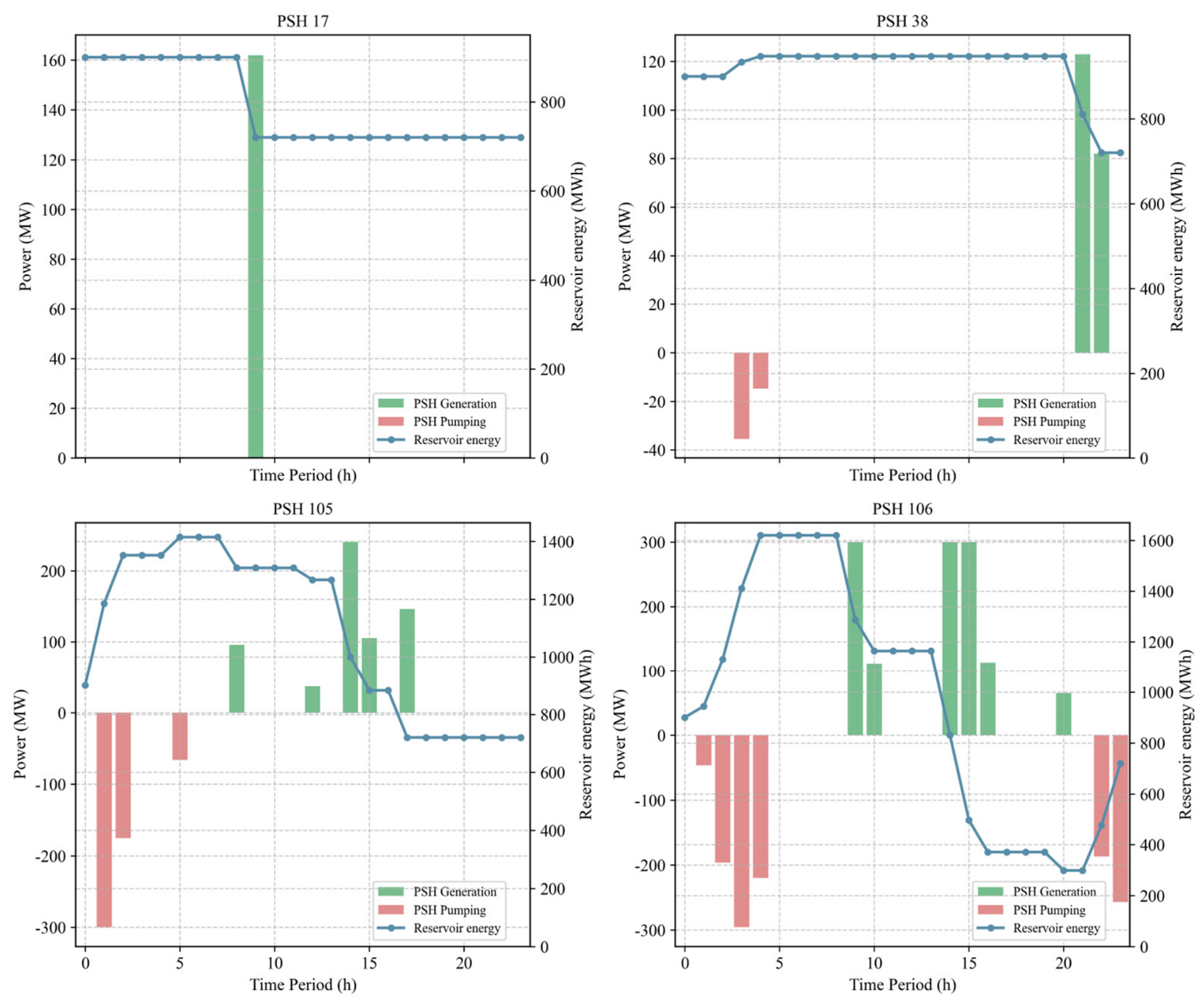
Based on the operational characteristics of pumped storage power and reservoir energy data for the base scenario shown in Figure 1, the following regularities can be summarized.

Operational characteristics of zonal pumped storage: The pumped storage unit in Zone 2 (PSH 17) only generates power (no pumping): it generates 162 MW at 9 h and remains off in other periods; its reservoir energy drops from 900 MWh to 720 MWh and then stays constant, indicating a net release of 180 MWh used for a single peak-shaving discharge before the evening peak. The unit in Zone 1 (PSH 38) both pumps and generates: pumping occurs at 3 h (35.44 MW) and 4 h (14.81 MW), while generation occurs at 21 h (122.93 MW) and 22 h (82.04 MW); its reservoir energy first rises from 900 MWh to 947.74 MWh (4 h) and then falls to 720 MWh (22 h), with a net release of about 227.74 MWh, playing a peak shaving regulation role of storing a small amount of energy at midday and discharging during the evening peak. The two units in Zone 3 (PSH 105 and PSH 106) are the main storage and discharge facilities. PSH 105 pumps at 1 h (300 MW), 2 h (175.49 MW) and 5 h (66.02 MW), and generates at 8 h (95.86 MW), 12 h (37.10 MW), 14 h (240.48 MW), 15 h (105.51 MW) and 17 h (146.03 MW); its reservoir energy rises from 900 MWh to 1414.43 MWh (5 h) and then drops to 720 MWh (17 h), a net release of about 694.43 MWh. PSH 106 pumps at 1 h (46.23 MW), 2 h (196.14 MW), 3 h (295.77 MW), 4 h (219.76 MW), 22 h (186.44 MW) and 23 h (256.67 MW), and generates at 9 h (300 MW), 10 h (111.08 MW), 14 h (300 MW), 15 h (300 MW), 16 h (112.80 MW) and 20 h (64.97 MW); its reservoir energy rises from 900 MWh to 1620 MWh (4 h), then after multiple discharge periods, drops to 720 MWh (23 h), a net release of about 900 MWh. Overall, the Zone 3 units store energy during renewable (wind and solar) surplus periods and discharge during load peaks.

Temporal patterns of pumped storage energy shifting: During the early morning to morning (0–7 h), when wind output is high, the Zone 3 units intensively pump: PSH 105 pumps at 1 h, 2 h, and 5 h (total 541.5 MWh), PSH 106 pumps at 1–4 h (total 757.9 MWh), and their reservoir energy rises to 1414.43 and 1620 MWh, respectively. During this period, PSH 38 also pumps a small amount at 3–4 h (about 50.25 MWh). No pumped storage generates. In the morning (8–12 h), load increases and PV starts to contribute; Zone 3 units begin to generate: PSH 105 generates at 8 h and 12 h (total 132.97 MWh), and PSH 106 generates at 9 h and 10 h (total 411.08 MWh); accordingly, the reservoir energy of PSH 105 drops from 1414.43 to 1266.69 MWh, and that of PSH 106 drops from 1620 to 1163.25. PSH 17 generates 162 MW at 9 h, reducing its reservoir energy to 720. In the afternoon to evening (14–19 h), PV declines, and the evening peak arrives; Zone 3 units generate heavily: PSH 105 generates at 14 h, 15 h, and 17 h (total 492.02 MWh), and PSH 106 generates at 14 h, 15 h, and 16 h (total 712.8 MWh); and, meanwhile, PSH 38 generates at 21–22 h (about 204.97 MWh). During this period, the reservoir energy of Zone 3 units keeps falling, with PSH 105 reaching 720 after 17 h and PSH 106 dropping to 371.24 at 16 h. At night (20–23 h), wind output recovers; PSH 106 pumps again at 22 h and 23 h (total 443.11 MWh) and generates a small amount at 20 h (about 64.97 MW), finally returning its reservoir energy to 720. PSH 105 has no action at night and stays at 720. Notably, the pumping of PSH 106 at 22–23 h follows the generation of PSH 38 at 21–22 h, forming a temporal succession without direct energy complementarity. PSH 106’s night pumping utilizes the recovered wind power for energy storage to achieve a daily cycle (final reservoir energy back to 720 MWh), whereas PSH 38’s evening generation plays a peak-shaving role.

In the base scenario, the operation modes of the four pumped storage units closely match their zonal roles: the Zone 2 unit (17) generates only once during the load peak, serving as a peaking unit; the Zone 1 unit (38) pumps a small amount at midday and generates in the evening, performing peak-shaving functions; and the two Zone 3 units (105 and 106) undertake the main tasks of storing renewable energy and discharging during load peaks. Their charging/discharging timings correspond to wind/PV surplus periods and load peak periods, respectively; moreover, PSH 106 pumps again at night when wind output recovers to maintain the daily cycle. The reservoir energy variations reveal the temporal coupling characteristics of cross-period energy shifting: storing in early morning → discharging before noon and in the afternoon → storing again at night, effectively smoothing renewable fluctuations and supporting the evening peak load. These regularities validate that the proposed model can correctly reflect the adaptive dispatch behavior of pumped storage based on zonal roles and transmission section constraints.

4.3.2. Zonal Power Exchange

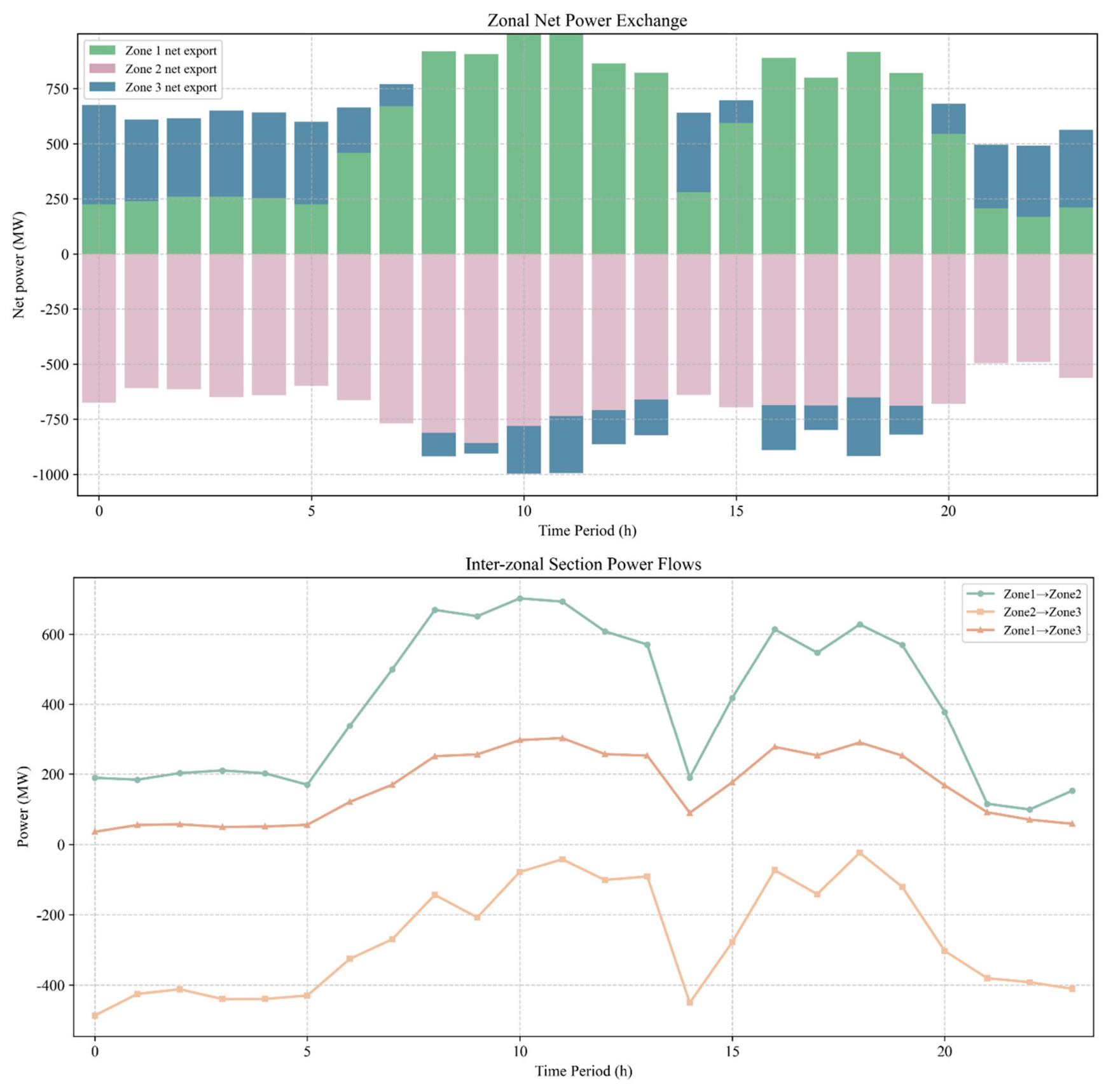
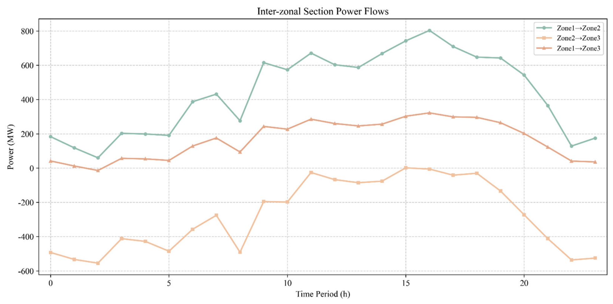
Based on the 24 h zonal power exchange data of the base scenario shown in Figure 2, the following regularities can be summarized.

Characteristics of zonal net power balance: Zone 1 (hub zone) is a net exporter throughout all periods, with a cumulative net export of 13,527.89 MWh and an hourly net export ranging from 169.20 MW (22 h) to 998.29 MW (10 h); the daily peak occurs at 10 h (morning load peak). Zone 2 (load center) is a net importer in all periods, with a cumulative net import of 16,066.02 MWh and an absolute hourly net import ranging from 490.97 MW (22 h) to 858.91 MW (9 h); the maximum net import of 858.91 MW appears at 9 h, indicating the load center’s dependence on power import through transmission. Zone 3 (renewable-rich zone) shows fluctuating behavior: net export from early morning to morning (0–7 h, highest 451.03 MW), shifts to net import during 8–13 h (maximum import 259.41 MW), returns to short-term net export during 14–15 h, changes again to net import during 16–19 h, and recovers to net export during 20–23 h. The cumulative net export of 2538.13 MW indicates that Zone 3 is a net exporter overall. The net import occurring in the evening is related to the sharp decline in PV output and the overlapping evening peak load.

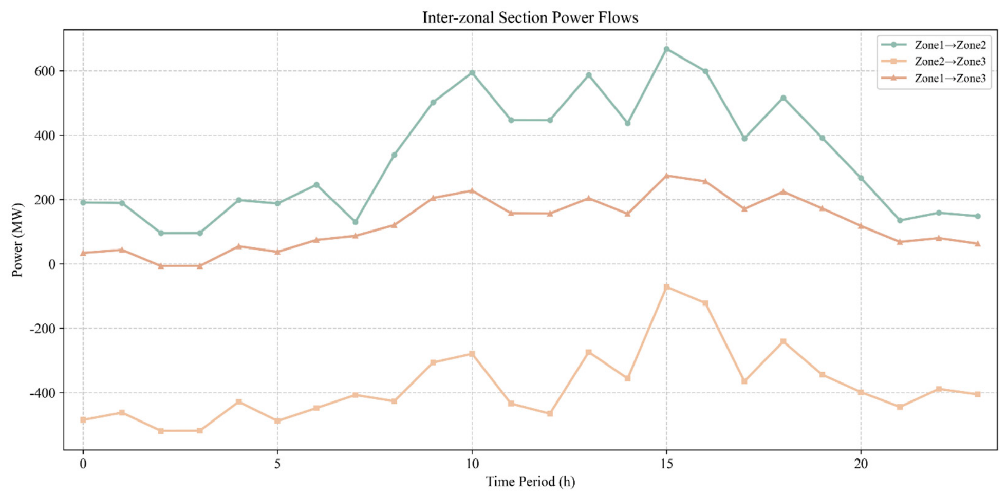
Characteristics of inter-zonal section power flows: The power flow directions on all three inter-zonal sections are fixed: the Zone 1 → Zone 2 section is always positive (power flows from Zone 1 to Zone 2), ranging from 99.08 MW (22 h) to 702.02 MW (10 h), with a daily average of about 399.89 MW; the Zone 2 → Zone 3 section is always negative (power flows from Zone 3 to Zone 2), with absolute values ranging from 23.75 MW (18 h) to 486.64 MW (0 h) and a daily average of about 269.53 MW; and the Zone 1 → Zone 3 section is always positive (power flows from Zone 1 to Zone 3), ranging from 35.61 MW (0 h) to 302.16 MW (11 h) and a daily average of about 163.77 MW. The absolute power on the Zone 2 → Zone 3 section is large during early morning and evening, and becomes very close to zero at midday (only 23.75 MW at 18 h), reflecting that the delivery capability of Zone 3 is significantly influenced by renewable output. The power on the Zone 1 → Zone 2 section rises rapidly before noon, synchronized with the morning load peak of Zone 1.

Temporal variation patterns:

(i)

During the early morning to early morning (0–5 h), wind power output is high: Zone 3 net exports 370–451 MW, Zone 2 net imports about 600–676 MW, and Zone 1 net exports 225–259 MW. At this time, the section powers are relatively low on Zone 1 → Zone 2 (169–210 MW), large in absolute value on Zone 2 → Zone 3 (412–487 MW), and small on Zone 1 → Zone 3 (35–57 MW). The system is mainly supplied by wind power from Zone 3, which is transmitted through the hub Zone 1 to Zone 2.

(ii)

From morning to noon (6–13 h), load increases and PV output rises. Zone 3 becomes a net importer from 8 h onward (maximum import 259 MW), Zone 1’s net export rapidly increases to 998 MW (10 h), and Zone 2’s net import also rises to 859 MW (9 h). On the sections, the power on the Zone 1 → Zone 2 section increases to 338–702 MW, the absolute value on the Zone 2 → Zone 3 section drops sharply to 42–101 MW, and the power on the Zone 1 → Zone 3 section rises to 250–302 MW. This indicates that during this period, Zone 1 not only directly sends power to Zone 3 to compensate for the power deficit caused by low wind output in Zone 3 but also sends power to Zone 2 to meet the increasing load demand in Zone 2.

(iii)

In the afternoon to evening (14–19 h), PV output declines. Zone 3 briefly exports during 14–15 h (360 MW and 102 MW) but then switches back to net import during 16–19 h (111–266 MW). The power on the Zone 1 → Zone 2 section first increases and then decreases (189–627 MW), the absolute value on the Zone 2 → Zone 3 section first decreases and then increases (450–24 MW), and the power on the Zone 1 → Zone 3 section stays in the range of 89–289 MW, showing bidirectional power exchange between Zone 3 and Zones 1 and 2.

(iv)

During the night (20–23 h), wind power output recovers. Zone 3 net export rises from 136 MW to 352 MW, and Zone 1 net import falls from 545 MW to 211 MW. On the sections, the power on the Zone 1 → Zone 2 section drops to 99–377 MW, the absolute value on the Zone 2 → Zone 3 section rises again to 303–411 MW, and the power on the Zone 1 → Zone 3 section stays at 58–167 MW. The system returns to the pattern where Zone 2 is mainly supplied by Zone 1 and Zone 3.

Under the base scenario, the zonal net power balance shows that Zone 2 is always a receiving end, Zone 1 is always a sending end, and the net power direction of Zone 3 fluctuates with renewable output, though cumulatively it is a net exporter. All inter-zonal section power directions are fixed (Zone 1 → Zone 2 and Zone 1 → Zone 3 are positive, Zone 2 → Zone 3 is negative), but their magnitudes vary significantly over time; notably, the power on the Zone 2 → Zone 3 section approaches zero at midday, reflecting that the mismatch between renewable generation and load in the renewable-rich zone causes a power reversal at that time. Temporally, the system relies on wind power exported from Zone 3 during early morning, switches to a pattern where Zone 1 uses its own thermal/pumped storage capacity and even sends power back to Zone 3 during the midday load peak, and then returns to the export pattern during the night. These regularities validate that the proposed model correctly captures the zonal functional roles and the temporal coupling characteristics of inter-zonal section powers.

4.3.3. Power Generation Structure

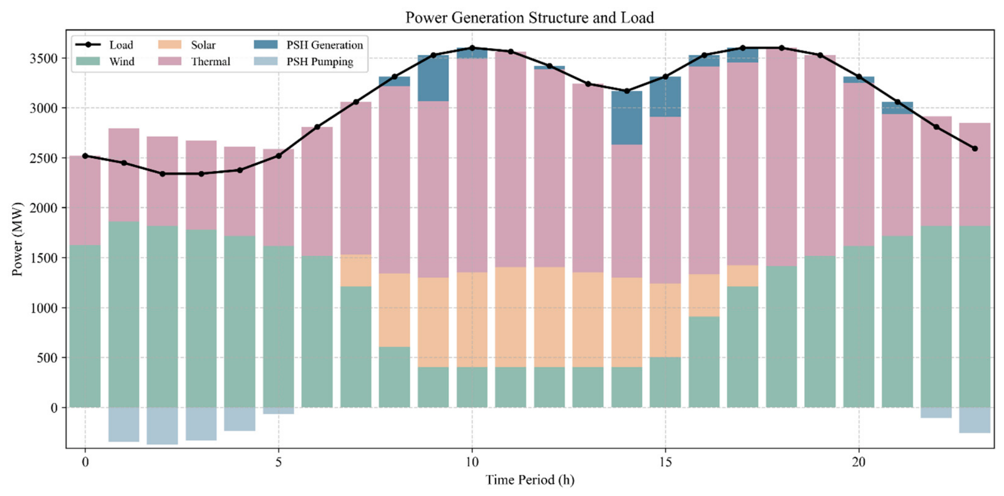
By the power generation structure based on wind-PV-thermal-PSH classification for the base scenario shown in Figure 3, the following regularities can be summarized.

The total system load over the 24 h horizon is 73,587.79 MWh. Zone 3 is the main clean energy supplier, equipped with large-scale wind and PV capacities. Wind output varies between 404.21 MW (midday) and 1859.37 MW (early morning), while PV peaks at 1000.00 MW around noon. The two PSH units in this zone perform intensive energy storage during periods of renewable surplus. The net effect is that Zone 3 stores excess wind energy during early morning (0–5 h) and night (22–23 h), and releases it during daytime peak hours, thereby smoothing renewable output and reducing thermal ramping requirements. Zone 2 is the primary load center with high load density. It relies on power imports from Zone 1 and Zone 3. Its PSH unit (PSH 17) operates only in generation mode: it generates 162.00 MW at 9 h (morning peak), discharging 180.00 MWh from its reservoir. This single discharge supports the morning load peak, demonstrating a peaking rather than a diurnal storage function. Zone 1 serves as the power transfer hub between Zone 2 and Zone 3. Its PSH unit (PSH 38) provides evening peak shaving and partially compensates for the reduction in renewable output after sunset.

A Temporal Coordination Summary is given below:

(i)

Early morning (0–5 h): High wind output, zero PV, low load. Zone 3 PSH units pump heavily (PSH 105: 541.51 MWh; PSH 106 during 1–4 h: 757.90 MWh; total ~1299.41 MWh). Zone 3 is a net exporter, supplying power via Zone 1 to Zone 2.

(ii)

Morning (8–12 h): Load rises to the daily peak, and PV output increases. Zone 3 PSH units start generating (PSH 105 at 8 h and 12 h: 132.97 MWh; PSH 106 at 9 h and 10 h: 411.08 MWh). Zone 2’s PSH 17 provides an additional 162.00 MW at 9 h. Zone 3 turns into a net importer, receiving power from Zone 1.

(iii)

Afternoon to evening (14–19 h): PV drops to zero, wind gradually recovers. Zone 3 PSH units discharge heavily (PSH 105: 492.02 MWh; PSH 106: 712.80 MWh). Zone 3 briefly becomes a net exporter but returns to net import during 16–19 h. Thermal generation ramps up to its evening peak (2185.45 MW at 18 h).

(iv)

Night (20–23 h): Wind output recovers to a high level. PSH 106 pumps again at 22–23 h (443.11 MWh) to restore its reservoir energy for the next day’s cycle. Zone 3 returns to net export, and thermal output decreases.

The power generation structure is dominated by wind (39.01%) and thermal (49.44%), with PV (11.01%) providing daytime support. The PSH units (net energy contribution of only 0.53%) play a critical flexibility role: Zone 3 units perform diurnal energy shifting, Zone 1’s unit offers evening peak shaving, and Zone 2’s unit supplies a morning peak. This classification validates that the coordinated operation of wind, PV, thermal, and PSH across three functional zones can effectively balance renewable variability and load following.

In the base scenario, the three zones have clear functional divisions: Zone 3 uses pumped storage to shift early morning wind power (and limited midday solar) to daytime peak hours (with brief reverse import at midday); Zone 1 relies on local thermal and pumped storage to support its load and even sends power back to Zone 3 when renewable energy is insufficient; Zone 2, as the load center, receives power from Zone 3 and Zone 1. The charging/discharging timing of pumped storage precisely matches the transition between renewable surplus and deficit (storage in early morning → discharge during daytime → re-storage at night). Thermal units provide regulation and reserve during high-load periods. These results validate that the proposed model correctly captures the temporal coordination characteristics among multiple zones, multiple pumped storage units, wind power, solar power, and thermal power.

5. Discussion

5.1. Core Indicator Comparison of Five Scenarios

Table 4. Operational indicators for five scenarios.

Scenario	Wind Installed Capacity (MW)	Thermal Generation (MWh)	Wind Generation (MWh)	Renewable Penetration (%)	Total Curtailment (MWh)	Curtailment Rate (%)	System Operation Cost ($)
A	2400	36,385.04	28,709.44	50.03	292.67	0.7887	1,887,316.44
B	2400	37,074.53	28,121.59	49.23	880.52	2.3729	1,919,907.16
C	2400	36,324.33	28,709.44	50.03	292.67	0.7887	1,884,384.27
D	1920	41,690.55	23,201.68	42.54	0.00	0.00	2,142,087.44
E	2880	32,852.15	32,417.32	55.07	2385.21	5.5589	1,717,112.77

reports the core operational indicators for five scenarios, including wind installed capacity, thermal generation, wind generation, renewable penetration, total curtailment, curtailment rate, and system operation cost.

Scenarios A–C share the same wind capacity (2400 MW) but differ in tie-line capacity: Scenario 1 (baseline, 500 MW), Scenario B (400 MW), and Scenario C (600 MW). As shown in Table 4, when the tie-line is tightened (Scenario B), the reduced transmission capability leads to higher wind curtailment: the curtailment rate rises from 0.79% to 2.37%. Consequently, thermal generation increases by 1.90% and system operation cost rises by 1.73%. When the tie-line is relaxed (Scenario C, 600 MW), the curtailment rate remains unchanged from the baseline (0.79%), with a slight cost reduction from 1,887,316.44 $ to 1,884,384.27 $. The limited improvement indicates diminishing marginal benefits once the tie-line capacity exceeds a critical value. With pumped storage deployed, the plant in the renewable-rich zone can store curtailed energy (using the curtailed power for pumping) during congested periods and generate later when the tie-line is less loaded or during peak load, effectively increasing the cross-zone transmission capability.

Scenarios A, D, and E maintain the same tie-line capacity (500 MW) while varying wind installed capacity: Scenario 1 (2400 MW, baseline), Scenario D (−20%, 1920 MW), and Scenario E (+20%, 2880 MW). From Table 4, when wind capacity is reduced by 20% (Scenario D), renewable penetration drops to 42.54% with zero curtailment (0.00%). However, thermal generation increases substantially (+14.59%) and system cost soars (+13.50%). The role of pumped storage weakens, but it can still replace some thermal peaking capacity. When wind capacity is increased by 20% (Scenario E), renewable penetration rises to 55.07%, the curtailment rate reaches 5.56%, total curtailed energy is 2385.21 MWh, and system cost decreases significantly (−9.02%). Under this high-penetration condition, pumped storage is urgently needed to absorb the curtailed energy.

5.2. Tie-Line Transmission Capacity Sensitivity Analysis

5.2.1. Variation Characteristics of Inter-Zonal Power Exchange in Scenarios A, B, and C

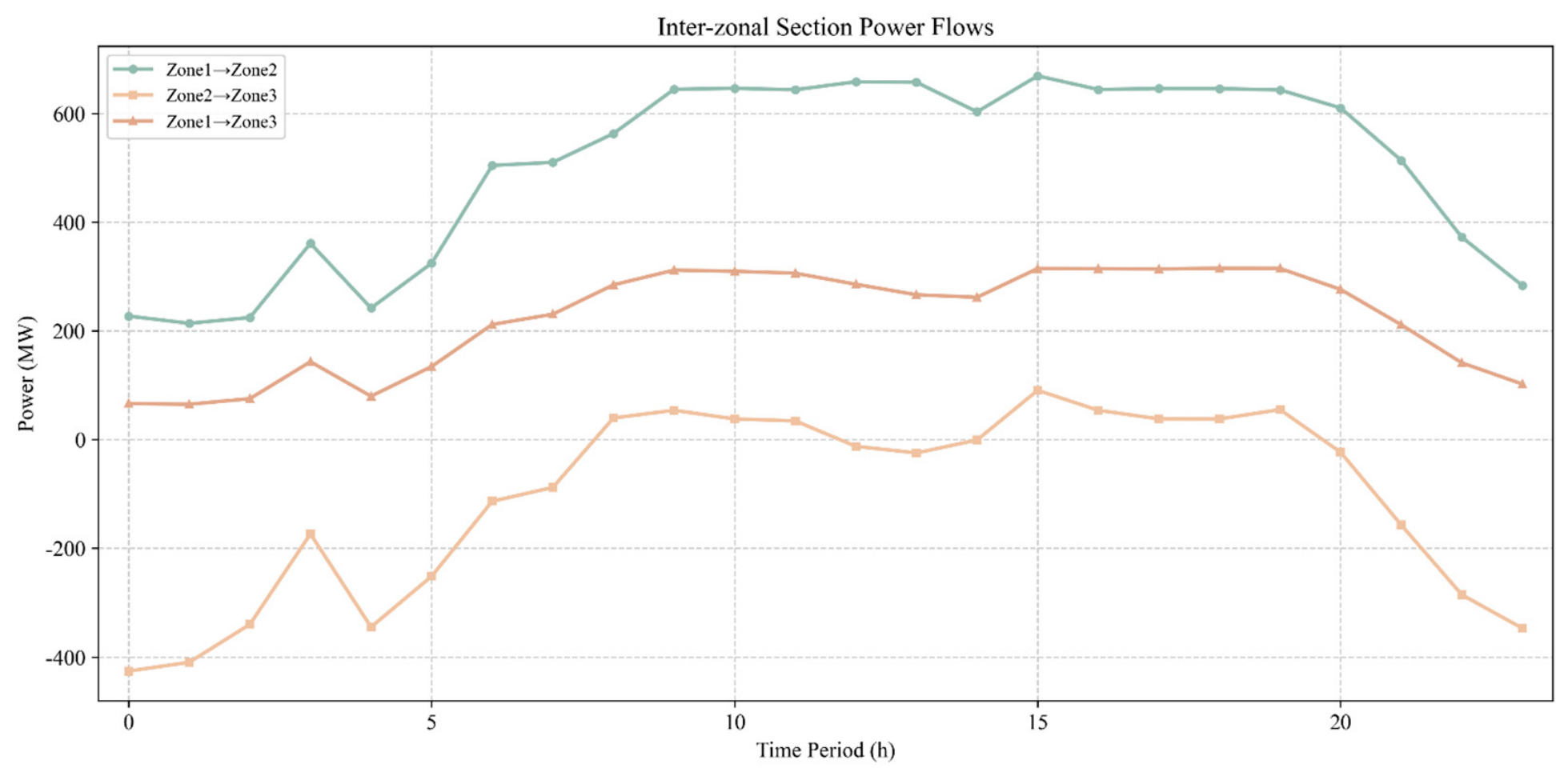
With the installed wind power capacity fixed at 2400 MW, the adjustment of tie-line capacity significantly changes the magnitude and fluctuation range of cross-zonal power flow, while the daily variation trend of inter-zonal power exchange remains essentially unchanged among the three scenarios.

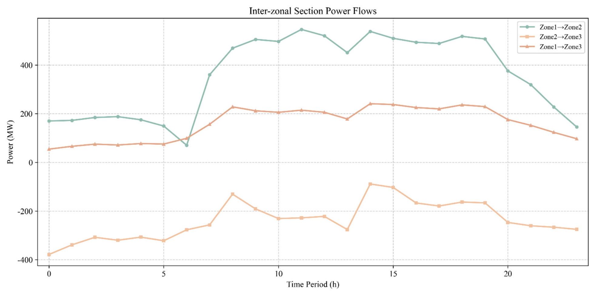
Figure 4 shows operational characteristics of zonal power exchange for Zones 1, 2 and 3 in Scenario B. In Scenario B, with the tie-line capacity tightened to 400 MW, inter-zonal transmission channels are subject to rigid constraints. Comparison of hourly data with Scenario A shows that the power from Zone 1 to Zone 2 decreases from 189.13 MW to 170.20 MW at Hour 0, and drops from 183.76 MW to 172.54 MW at Hour 1. Such differences are widely observed during daytime peak hours (8:00–19:00). The hourly transmission power from Zone 1 to Zone 2 and Zone 1 to Zone 3 in Scenario B is generally lower than that in the benchmark scenario. In terms of net outgoing power, the net outgoing power of Zone 2 is −675.77 MW in Scenario A and −548.38 MW in Scenario B at Hour 0, indicating a clear reduction in the absolute value of net incoming power of Zone 2. Restricted by insufficient transmission channels, surplus power generated in renewable-energy-rich zones cannot be delivered outward timely, resulting in local power accumulation and aggravated wind curtailment. During the peak delivery period of 8:00–19:00, the maximum net outgoing power of Zone 1 reaches 919.45 MW in Scenario A, while the corresponding value is only 779.07 MW in Scenario B. The outward delivery capability of Zone 1 is clearly suppressed, which fully reflects the bottleneck effect of tie-line capacity on cross-zonal power transmission.

Figure 5 shows operational characteristics of zonal power exchange for Zones 1, 2 and 3 in Scenario C. In Scenario C, with the tie-line capacity relaxed to 600 MW, the transmission margin of inter-zonal channels is improved. The power flow of each channel is highly consistent with that in Scenario A. At Hour 0, the power from Zone 1 to Zone 2 is 183.29 MW and the net outgoing power of Zone 1 is 224.73 MW, both nearly equal to the benchmark values. At Hour 11, the net outgoing power of Zone 1 is 956.07 MW, which has a small deviation from 994.78 MW in the benchmark scenario. On the whole, the variation in hourly exchange power of each channel and net outgoing power of each zone is negligible. It demonstrates that when the tie-line capacity exceeds the critical value matching power output and load level, further capacity expansion presents diminishing marginal benefits for cross-zonal power flow optimization and renewable energy accommodation. The tie-line no longer acts as the main constraint for inter-zonal power mutual support, and only minor adjustments occur in inter-zonal power exchange.

The daily temporal characteristics of power flow are highly uniform under the three tie-line configurations. During 0:00–7:00 and 20:00–23:00, the net outgoing power of Zone 3 remains positive. Taking Hour 0 as an example, the net outgoing powers of Zone 3 are 451.03 MW, 323.64 MW and 451.03 MW in Scenarios A, B and C respectively. Zone 2 maintains negative net outgoing power and undertakes the role of load center. During 8:00–19:00, the power flow direction reverses, the net outgoing power of Zone 3 turns negative, and the net outgoing power of Zone 1 rises sharply, making Zone 1 the dominant power delivery source. A typical time-divided and zone-divided power supply–demand pattern is formed, and this temporal power flow characteristic is not affected by tie-line capacity adjustments.

5.2.2. Operational Patterns of Pumped Storage Units in Scenarios A, B, and C

In Scenario A, the pumped storage units mainly perform peak shaving and valley filling, exhibiting a clear separation between charging (pumping) and discharging (generating) periods.

• Unit PSH 17 (Zone 2): Generates only at hour 9 (162 MW) for the morning peak, with no pumping. Its stored energy decreases from 900 MWh to 720 MWh and then remains constant.
• Unit PSH 38 (Zone 1): Pumps only at hours 3–4 (35.44 MW and 14.81 MW). Its stored energy rises from 900 MWh to 947.74 MWh, indicating absorption of surplus wind power during off-peak hours.
• Unit PSH 105 (Zone 3): Generates during the daytime (hours 8, 12, 14, 15, 17), with a peak of 240.48 MW (hour 14); pumps during the night and early morning (hours 1–2, 5), with a peak of 300 MW (hour 1). Its stored energy rises through pumping to the upper limit of 1414.43 MWh, then decreases to 720 MWh through generation.
• Unit PSH 106 (Zone 3): Generates at hours 9, 10, 14, 15, 16, 20 (maximum 300 MW); pumps at hours 1–4 and 22–23 (maximum 295.77 MW). Its stored energy increases from 900 MWh to 1620 MWh (fully charged at hour 4), then discharges to 720 MWh (at hour 23).

Under the base scenario, the pumped storage units follow a classic daily cycle—charging during low-load, high-wind night hours and discharging during daytime peak hours. The units in Zone 3 (PSH 105 and PSH 106) are highly utilized, while PSH 17 plays a minor role.

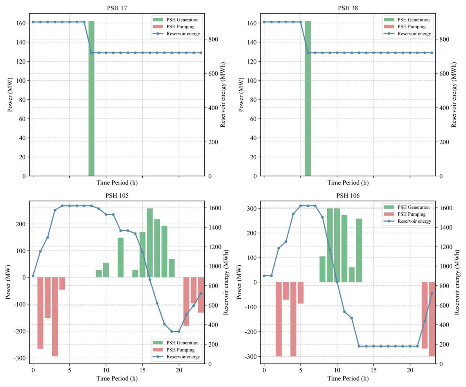
Figure 6 shows operational characteristics of zonal pumped storage for PSH 17/38/105/106 in Scenario B. Under tightened transmission capacity (400 MW), cross-zone power exchange is restricted, leading to increased curtailment risk. Pumped storage operation adapts accordingly.

• PSH 17: Generates 162 MW at hour 8 (morning peak)—similar to Scenario A, with no pumping.
• PSH 38: Generates 162 MW at hour 6 (early morning), which is a new operating point compared to Scenario A (where PSH 38 only pumped). Its reservoir energy drops from 900 MWh to 720 MWh at hour 6 and remains at that level. This indicates that under the constrained tie-line condition, Zone 1 cannot import surplus renewable power and uses pumped storage to convert the excess renewable energy into stored energy.
• PSH 105: Pumps heavily during hours 1–4 (265.40 MW, 152.10 MW, 294.12 MW, 46.28 MW) and generates during hours 9–19 (multiple periods, with a maximum of 257.71 MW at hour 16). Its reservoir energy rises to 1620 MWh (fully charged) by hour 4, then gradually discharges to 720 MWh by hour 23.
• PSH 106: Pumps during hours 2–5 and 22–23 (maximum 300 MW), and generates during hours 8–13 (maximum 300 MW). Its reservoir energy increases from 900 MWh to 1620 MWh by hour 5; after generation, it drops to 180 MWh at hour 13 and remains low until hour 22, when it slightly recharges.

Under tie-line constraint, pumped storage units operate more aggressively in both charging and discharging to compensate for limited cross-zone power transfer. The reservoir energy profiles show deeper discharge (e.g., PSH 106 down to 180 MWh) and higher cycling intensity. This helps absorb wind curtailment during off-peak hours and supply local load during peak hours, effectively substituting for missing transmission capacity.

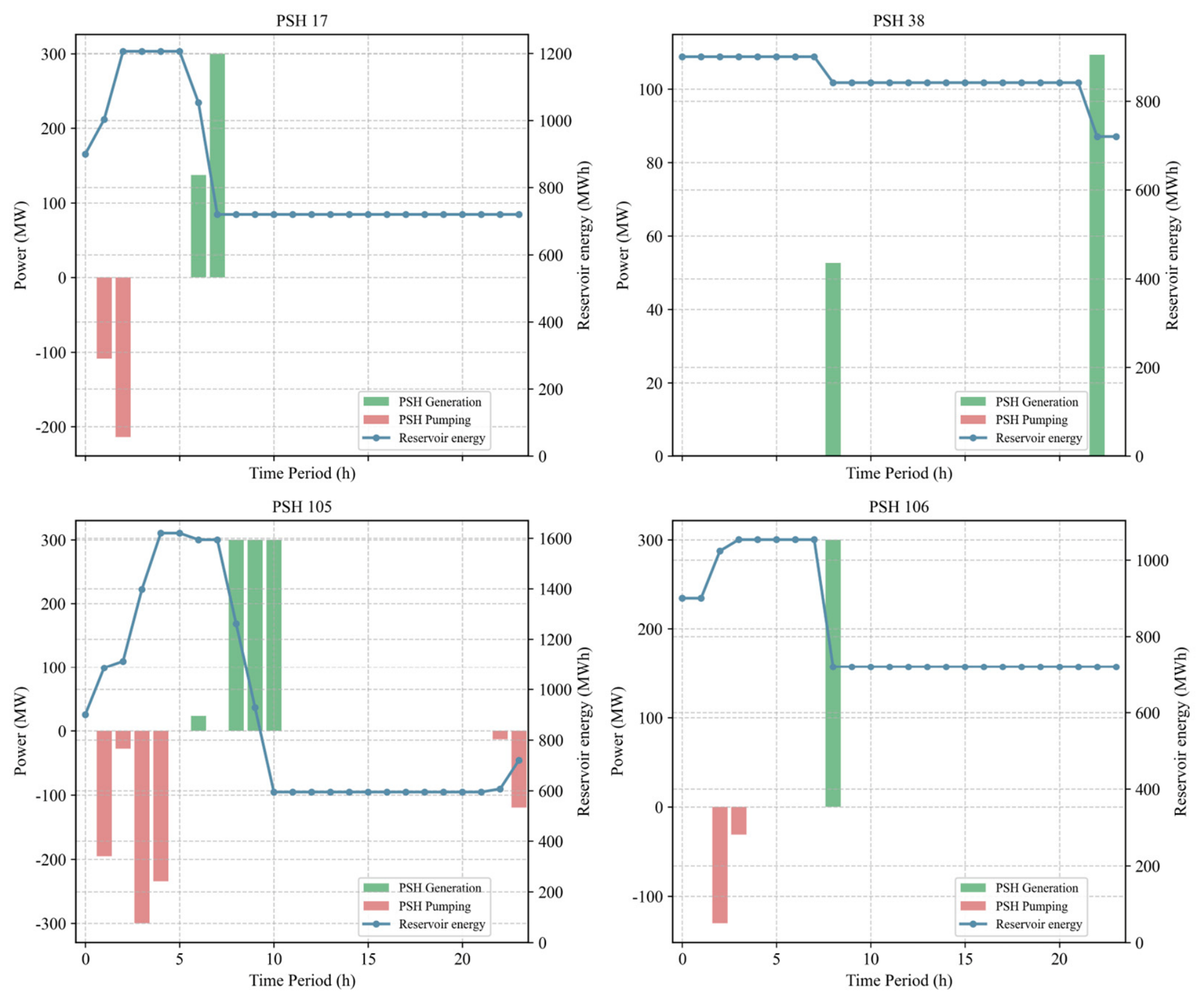
Figure 7 shows operational characteristics of zonal pumped storage for PSH 17/38/105/106 in Scenario C. With a more relaxed tie-line capacity (600 MW), cross-zone power exchange is less restricted, reducing the need for intensive pumped storage regulation.

• PSH 17: Pumps during hours 1–2 (108.49 MW and 213.66 MW) and generates during hours 6–7 (137.44 MW and 300 MW). Its reservoir energy increases from 900 MWh to 1206 MWh (pumping) and then decreases to 720 MWh after generation. This is a clear daily cycle.
• PSH 38: Generates 52.63 MW at hour 8 and 109.37 MW at hour 22, with no pumping. Its reservoir energy decreases slightly from 900 MWh to 841.52 MWh after generation, and then remains constant.
• PSH 105: Pumps during hours 1–4 (195.55 MW, 27.77 MW, 300 MW, 234.57 MW) and generates at hours 6, 8, 9, and 10 (maximum 300 MW). Its reservoir energy rises to 1620 MWh by hour 4, then discharges to 594 MWh by hour 10 and stays at that level until hour 21. During hours 22–23, it pumps 12.97 MW and 119.61 MW, and its reservoir energy jumps to 720 MWh.
• PSH 106: Pumps during hours 2–3 (130.19 MW and 31.21 MW). Its reservoir energy increases from 900 MWh to 1053 MWh. At hour 8, it generates 300 MW, and its reservoir energy drops to 720 MWh.

With a relaxed tie line, pumped storage operation becomes less intense compared to Scenario B. Charging and discharging are more balanced, and units do not deplete reservoir energy to extremely low levels (PSH 106 stays above 720 MWh after hour 8). The system relies more on cross-zone power transfer rather than local storage.

Table 5. Synergistic rules of tie-line transmission capacity and pumped storage operation.

Indicator	Unit	Scenario A	Scenario B	Scenario C
Total daily pumping (TDP)	MWh	1792.76	2493.76	1374.03
Total daily generation (TDG)	MWh	2180.81	2780.16	1822.80
Minimum reservoir energy (MRE)	MWh	299.05	180	594.04
Maximum reservoir energy (XRE)	MWh	1620	1620	1620
Curtailed renewable energy (CRE)	MWh	292.67	880.52	292.67
Curtailment rate (CR)	%	0.7887	2.3729	0.7887
PSH operation		Peak shaving	Deep discharge	Peak shaving

gives synergistic rules of tie-line transmission capacity and pumped storage operation. Six key operational indicators, including total daily pumping (TDP), total daily generation (TDG), minimum reservoir energy (MRE), maximum reservoir energy (XRE), curtailed renewable energy (CRE), and curtailment rate (CR), are used to analyze the impact of tie-line transmission capacity on pumped storage operation. The pumped storage units exhibit a clear dependency on tie-line capacity. Under base conditions (Scenario A), they follow a conventional daily charge–discharge cycle, storing excess wind energy at night and releasing it during daytime peaks. When the tie line is constrained (Scenario B), the units operate more aggressively—deeper discharge and more frequent cycling—to compensate for the limited cross-zone power exchange, thereby reducing renewable curtailment. When the tie line is relaxed (Scenario C), the operational intensity declines, and storage is used primarily for price arbitrage and grid stability, with reservoir energy remaining within a narrower band. These results demonstrate that pumped storage can effectively substitute for transmission capacity in multi-zone power systems, but its utilization factor and economic viability are highly sensitive to the degree of interconnection.

5.3. Installed Wind Power Capacity Sensitivity Analysis

5.3.1. Variation Characteristics of Inter-Zonal Power Exchange in Scenarios A, D, and E

With the tie-line capacity maintained at the benchmark value of 500 MW, the change in installed wind power capacity directly alters the power output of power-rich zones. Significant divergences in cross-zonal power flow distribution are observed according to the 24 h hourly exchange power data.

Figure 8 shows operational characteristics of zonal power exchange for Zones 1, 2 and 3 in Scenario D. In Scenario D, where the installed wind power capacity is reduced by 20% to 1920 MW, the overall output of renewable energy declines. The transmission power of all inter-zonal channels increases throughout the day. At Hour 0, the power from Zone 1 to Zone 2 is 227.01 MW, clearly higher than 189.13 MW in Scenario A. The power increment is more prominent during 8:00–19:00, with the net outgoing power of Zone 1 reaching 847.19 MW at Hour 8 and 949.31 MW at Hour 11. To make up for the shortage of wind power generation, thermal power output increases substantially, and Zone 1 becomes the main power delivery source of the system. In terms of power flow pattern, the net outgoing power of Zone 2 and Zone 3 keeps negative during 8:00–19:00. The direction of inter-zonal power flow tends to be single, the fluctuation range of power exchange decreases, and the pressure of cross-zonal power delivery is highly concentrated on Zone 1. Meanwhile, the reduction in wind power output eliminates wind curtailment, and surplus power in each zone is fully accommodated.

Figure 9 shows operational characteristics of zonal power exchange for Zones 1, 2 and 3 in Scenario E. In Scenario E, where the installed wind power capacity is increased by 20% to 2880 MW, the total output of renewable energy rises dramatically, and the power flow presents strong time-varying characteristics. During nighttime, with high wind power output (0:00–7:00, 20:00–23:00), the inter-zonal transmission power drops clearly. At Hour 0, the power from Zone 1 to Zone 2 is 190.80 MW, close to the benchmark value, while the net outgoing power of Zone 3 reaches 451.03 MW. At Hour 22, the power from Zone 1 to Zone 2 is only 158.71 MW, much lower than that in Scenario D. Restricted by tie-line capacity, a large amount of surplus wind power accumulates locally, leading to severe wind curtailment. During daytime load peak hours (8:00–19:00), the inter-zonal delivery power rebounds significantly. The net outgoing power of Zone 1 hits 942.42 MW at Hour 15, the maximum value among all scenarios, representing the peak outward delivery pressure of Zone 1. According to the hourly data, large-scale wind power integration further intensifies the time mismatch between power generation and load. The characteristics of surplus power in each zone at night and full-load cross-zonal transmission in the daytime are distinct, and the contradiction between local power surplus and cross-zonal transmission constraints becomes prominent.

5.3.2. Operational Patterns of Pumped Storage Units in Scenarios A, D, and E

To investigate the influence of wind power installed capacity on pumped storage unit operation, three typical scenarios are selected: Scenario A (wind power 2400 MW, baseline), Scenario D (wind power 1920 MW, reduced by 20%), and Scenario E (wind power 2880 MW, increased by 20%). Based on hourly wind power output, pumped storage unit charging/discharging power, and reservoir energy, the coupling relationship between wind power level and pumped storage regulation intensity is revealed.

(i)

Scenario A (Baseline Wind Power, 2400 MW)

Wind Power Output Characteristics: During nighttime (0–7 h), wind power output remains at a high level, ranging between 1212 MW and 1859 MW; it drops sharply in the early morning (8–9 h) to 606.32 MW and 404.21 MW; during the daytime (9–14 h), it stabilizes at 404.21 MW; and in the evening (15–23 h), it gradually recovers to 1818.95 MW. This exhibits a typical anti-peaking characteristic (high at night, low during the day).

Pumped Storage Operation: In Scenario A, PSH 17 in Zone 2 generates briefly at hour 9, while PSH 38 in Zone 1 pumps during early morning and generates in the evening. During the nighttime high-wind period, PSH 105 and PSH 106 pump heavily to absorb surplus wind power, converting electrical energy into hydraulic potential energy. During the daytime, when wind power output plummets, the pumped storage units generate intensively to compensate for the wind power deficit and meet the peak load. The charging/discharging schedule closely matches wind power fluctuations, effectively smoothing the net load curve.

(ii)

Scenario D (Wind Power Reduced by 20%, 1920 MW)

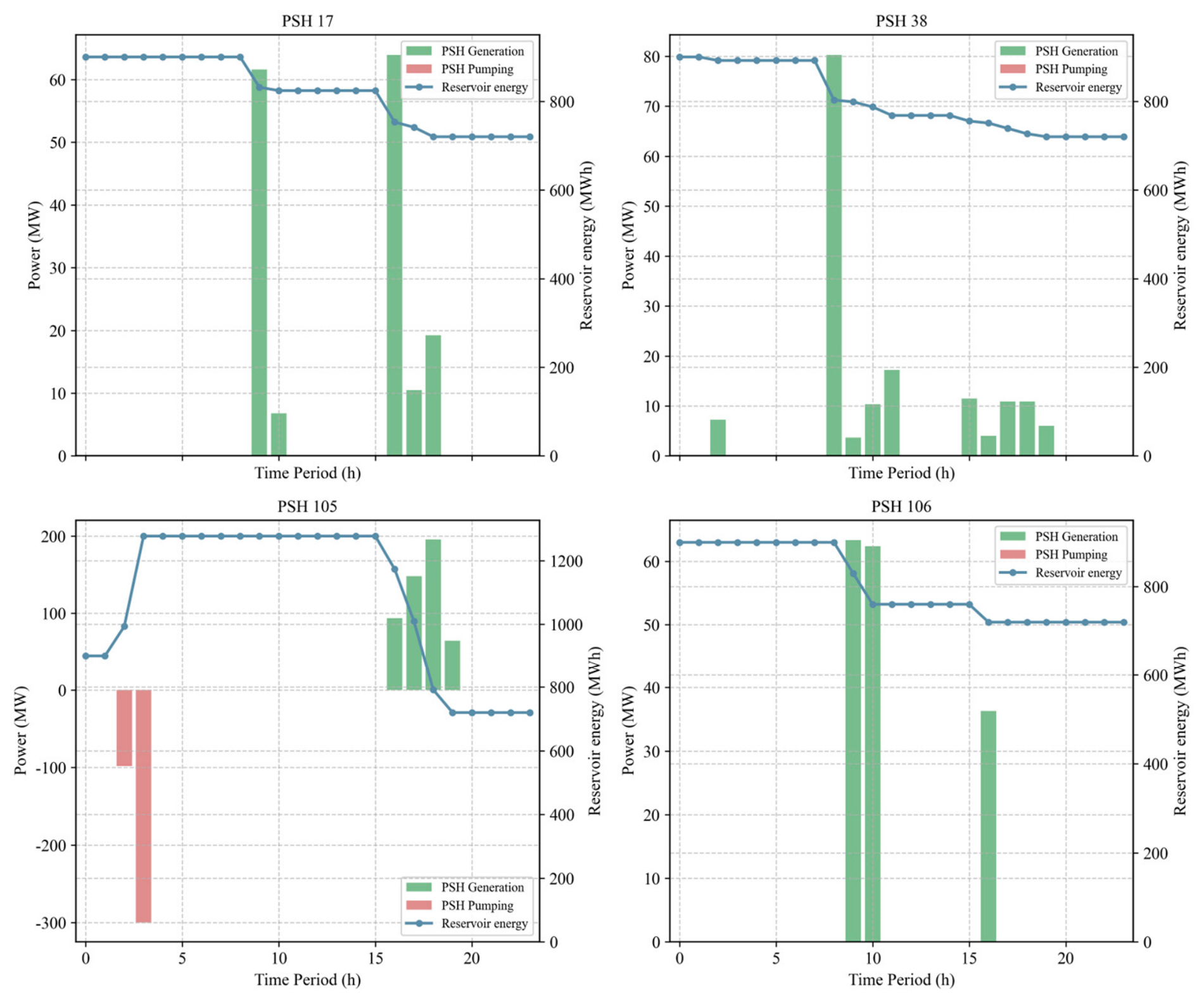
Figure 10 shows the operational characteristics of zonal pumped storage for PSH 17/38/105/106 in Scenario D.

Wind Power Output Characteristics: The overall output is approximately 20% lower than the baseline scenario. Nighttime output decreases from 1536 MW (hour 0) to 970.11 MW (hour 7); the daytime trough further drops to 323.37 MW (hours 9–14); and evening output recovers to 1455.16 MW (hours 22–23). The daily output is significantly reduced.

Pumped Storage Operation in Scenario D:

• Unit PSH 17: Generates a small amount during hours 9–10 (61.57 MW and 6.77 MW) and hours 16–18 (63.93 MW, 10.50 MW and 19.23 MW). Its reservoir energy drops from 900 MWh to 824.06 MWh, and then to 720 MWh.
• Unit PSH 38: Generates intermittently during hours 2–19 (peak 80.29 MW). Its reservoir energy decreases from 900 MWh to 720 MWh.
• Unit PSH 105: Pumps only during nighttime hours 3 and 4 (97.96 MW and 300 MW, respectively). Its reservoir energy rises from 900 MWh to 1278.06 MWh and remains constant until hour 15, then discharges during hours 16–19, and its reservoir energy drops to 720 MWh.
• Unit PSH 106: No pumping record. It generates 63.34 MW, 62.38 MW and 36.28 MW at hours 9, 10 and 16, respectively. Its reservoir energy stays at 900 MWh (hours 0–8) and then drops to 720 MWh by hour 16.

Due to low wind power output, there is no significant curtailment (curtailment rate ≈ 0). The need for curtailment absorption by pumped storage greatly diminishes. Only PSH 105 pumps once at night; the remaining units generate at very low power levels, primarily for daily peak shaving rather than curtailment mitigation. The total cycling energy of pumped storage is significantly lower than in the baseline scenario, indicating reduced utilization of energy storage under low wind power capacity.

(iii)

Scenario E (Wind Power Increased by 20%, 2880 MW)

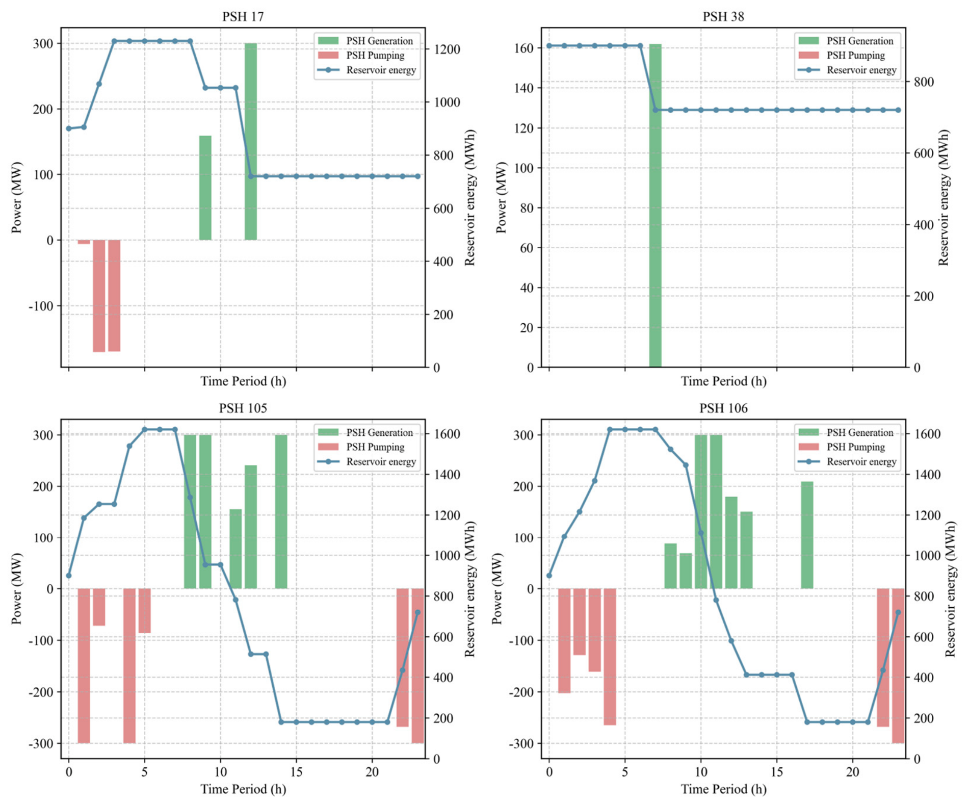
Figure 11 shows operational characteristics of zonal pumped storage for PSH 17/38/105/106 in Scenario E.

Wind Power Output Characteristics: Multiple nighttime peaks occur: 2064.44 MW at hour 1, 2048.15 MW at hour 4, and above 2150 MW at hours 22–23. The daytime trough remains at 485 MW (hours 9–14). Overall output is about 20% higher than the baseline scenario, with more intense fluctuations and a significantly increased risk of curtailment.

Pumped Storage Operation in Scenario E:

• Unit PSH 17: Pumps during hours 1–3 (6.16 MW, 170.68 MW, and 170.14 MW). Its reservoir energy rises from 900 MWh to 1229.64 MWh. It generates 158.67 MW at hour 9 and 300 MW at hour 12, and its reservoir energy drops to 720 MWh.
• Unit PSH 38: Generates only 162 MW at hour 7, with its reservoir energy decreasing from 900 MWh to 720 MWh.
• Unit PSH 105: Pumps intensively during hours 1–5 (300 MW at hour 1, 71.89 MW at hour 2, 300 MW at hour 4, and 86 MW at hour 5). Its reservoir energy rises from 900 MWh to the upper limit of 1620 MWh. It generates heavily during daytime hours 8–14 (300 MW at hour 8, 300 MW at hour 9, 155.46 MW at hour 11, 240.54 MW at hour 12, and 300 MW at hour 14), discharging its reservoir energy to 180 MWh (the deepest discharge among all scenarios). It pumps again during hours 22–23 (268.42 MW and 300 MW), recovering its reservoir energy to 720 MWh.
• Unit PSH 106: Pumps during hours 1–4 (202.96 MW at hour 1, 129.06 MW at hour 2, 161.06 MW at hour 3, and 264.82 MW at hour 4). Its reservoir energy rises from 900 MWh to 1620 MWh. It generates during daytime hours 8–13 and hour 17 (87.98 MW at hour 8, 68.89 MW at hour 9, 300 MW at hour 10, 300 MW at hour 11, 179.79 MW at hour 12, 150.45 MW at hour 13, and 208.89 MW at hour 17), discharging its reservoir energy to 180 MWh. It pumps again during hours 22–23 (268.42 MW and 300 MW), recovering its reservoir energy to 720 MWh.

From the above analysis of Scenarios A, D, and E, it is known that under high wind power capacity, nighttime wind output surges, creating substantial curtailment risk. Pumped storage units pump intensively during two periods (hours 1–5 and 22–23), absorbing surplus wind power, and reservoir energy generally reaches the upper limit (1620 MWh). During the daytime, when wind output is relatively low, pumped storage units generate at full capacity, and reservoir energy is deeply discharged to 180 MWh—lower than the baseline (720 MWh)—indicating that storage resources are fully utilized to replace thermal generation. The depth and frequency of charging/discharging cycles are significantly higher than in the baseline scenario, making pumped storage the core regulation means for curtailment absorption and power supply security.

The wind power level directly drives the pumped storage utilization intensity: Higher wind power capacity leads to more severe nighttime curtailment, which in turn increases the pumping power and cumulative pumping energy. Concurrently, daytime generation demand also rises, resulting in a significantly expanded reservoir energy range.

Pumped storage cycling depth is positively correlated with curtailment rate: In Scenario E, the reservoir energy lower limit drops to 180 MWh, much lower than in the baseline (720 MWh) and low-wind scenarios (720 MWh). This indicates that under high-curtailment conditions, storage resources are “squeezed” to the limit to enhance renewable integration.

Spatio-temporal matching characteristics: Pumped storage charging periods (nighttime and late night) strictly coincide with wind power peak periods; discharging periods (daytime) coincide with wind power troughs and peak load periods. This anti-phase regulation is the fundamental paradigm of wind-pumped storage synergy.

Marginal benefit of pumped storage diminishes under low wind power capacity: When wind power is reduced by 20% and the curtailment rate approaches zero, the curtailment-absorption function of pumped storage disappears, leaving only minor peaking support. Total cycling energy is less than 30% of the baseline, indicating that the economic viability of pumped storage heavily depends on the curtailment level.

Table 6. Synergistic rules of installed wind power capacity and pumped storage operation.

Indicator	Unit	Scenario A	Scenario D	Scenario E
TDP	MWh	1792.76	397.96	2999.62
TDG	MWh	2180.81	988.26	3212.67
MRE	MWh	299.05	720	180
XRE	MWh	1620	1278.06	1620
CRE	MWh	292.67	0	2385.21
CR	%	0.7887	0	5.5589
PSH Operation		Peak shaving	Peaking shaving	Renewable energy accommodation

gives synergistic rules of installed wind power capacity and pumped storage operation. The installed capacity of wind power has a decisive influence on the operational behavior of pumped storage. Under baseline wind power, pumped storage achieves a typical daily charge–discharge cycle, effectively smoothing the net load. When wind power is reduced by 20%, curtailment disappears, and the demand for pumped storage drops sharply, resulting in substantially lower utilization. When wind power is increased by 20%, pumped storage enters a deep-cycling mode, with pumping and generation powers and energy throughput significantly increased, and the reservoir energy lower limit is pulled down to 180 MWh, making pumped storage a critical resource for curtailment absorption and thermal generation replacement. These results demonstrate that in multi-zone power systems with high shares of renewable energy, the value of pumped storage grows nonlinearly with the curtailment rate, and its optimal capacity should be dynamically optimized based on typical curtailment scenarios.

5.4. PSP Capacity Sensitivity Analysis

To investigate the impact of pumped storage unit capacity on system operational performance, this subsection performs simulations under five typical scenarios (A–E) with four capacity schemes: 250 MW, 300 MW (baseline), 400 MW, and 425 MW. The effects of PSP capacity variations on six key operational indicators—TDP, TDG, MRE, XRE, CRE, and CR—are analyzed. Among these, 250 MW and 300 MW are the two most widely applied unit capacities in China’s pumped storage power stations, 400 MW has been practically implemented and operates reliably, and 425 MW represents the current record for the largest unit capacity in China. The simulation results for the four capacity schemes under the five scenarios are presented in

Table 7. Operational indicators under different capacity schemes across various scenarios.

Indicator	Scenario A				Scenario B				Scenario C				Scenario D				Scenario E
	250	300	400	425	250	300	400	425	250	300	400	425	250	300	400	425	250	300	400	425
TDP	1795.31	1792.76	1795.13	1795.13	2454.49	2493.76	2493.76	2493.76	1374.03	1374.03	1346.29	1374.03	420.22	397.96	397.96	397.96	2999.62	2999.62	2976.80	2999.62
TDG	2182.99	2180.81	2182.84	2182.84	2746.59	2780.16	2780.16	2780.16	1822.80	1822.80	1799.08	1822.80	1007.28	988.26	988.26	988.26	3212.67	3212.67	3193.17	3212.67
MRE	303.14	299.05	720.00	720.00	237.93	180.00	180.00	330.93	594.04	594.04	594.04	594.04	720.00	720.00	720.00	720.00	180.00	180.00	180.00	180.00
XRE	1612.50	1620.00	1557.28	1620.00	1620.00	1620.00	1620.00	1620.00	1582.30	1620.00	1608.89	1620.00	1112.93	1278.06	1278.06	1278.06	1620.00	1620.00	1620.00	1620.00
CRE	294.80	292.67	292.67	292.67	908.41	880.52	880.52	880.52	292.67	292.67	320.41	292.67	0	0	0	0	2386.49	2385.21	2407.53	2384.71
CR	0.7944	0.7887	0.7887	0.7887	2.448	2.3729	2.3729	2.3729	0.7887	0.7887	0.8635	0.7887	0	0	0	0	5.5619	5.5589	5.6109	5.5578

.

From Table 7, the following patterns can be summarized:

(i)

Capacity expansion has limited impact on PSP operational intensity under baseline conditions. In Scenario A (baseline), the variations in TDP and TDG across different capacity schemes are minimal, indicating that under the baseline configuration of 2400 MW wind power and 500 MW tie-line capacity, the existing 250 MW PSP capacity is already sufficient to absorb the available surplus renewable energy. Further capacity expansion does not increase PSP utilization, as the system’s renewable surplus is the binding constraint rather than PSP capacity.

(ii)

Capacity expansion has a more pronounced effect under tightened section constraints. In Scenario B (tightened section, 400 MW tie-line capacity), increasing PSP capacity from 250 MW to 300 MW increases TDP from 2454.49 MWh to 2493.76 MWh (a 1.60% increase) and TDG from 2746.59 MWh to 2780.16 MWh (a 1.22% increase), while the curtailment rate drops from 2.448% to 2.373% (a reduction of 0.075 percentage points). This indicates that under transmission-constrained conditions, a larger PSP capacity can partially compensate for the limited export capability by storing more surplus renewable energy locally. However, further increasing capacity from 300 MW to 400 MW or 425 MW yields no additional improvement—all indicators remain nearly identical to the 300 MW case. This suggests that 300 MW is the saturation point beyond which additional capacity provides no further benefit under the given section limit.

(iii)

Capacity expansion yields limited curtailment reduction benefits in most scenarios. In Scenario A, CRE remains nearly constant (294.80 MWh for 250 MW vs. approximately 292.67 MWh for 300–425 MW), indicating that once the PSP capacity reaches 250 MW, additional capacity contributes little to further curtailment reduction. In Scenario B, CRE decreases from 908.41 MWh (250 MW) to 880.52 MWh (300–425 MW), a reduction of approximately 27.89 MWh (3.07%), but no further reduction is observed beyond 300 MW. In Scenario E, CRE decreases slightly from 2386.49 MWh (250 MW) to 2384.71 MWh (425 MW), a reduction of only 1.78 MWh over a 175 MW capacity increase, confirming that the curtailment reduction benefit of capacity expansion is marginal and subject to diminishing returns.

(iv)

Capacity benefits are constrained by renewable availability and transmission limits. In Scenario D (wind capacity reduced by 20%), curtailment is zero across all capacity schemes, and TDP decreases as capacity increases (from 420.22 MWh at 250 MW to 397.96 MWh at 300–425 MW), indicating that when renewable energy is insufficient, larger PSP capacity is underutilized and does not provide any additional benefit. In Scenario E (wind capacity increased by 20%), the curtailment rate remains high across all capacity schemes (5.56–5.61%), and the differences among capacity schemes are negligible (CR varies by only 0.05 percentage points). This suggests that the primary limitations to curtailment reduction are not PSP capacity but rather the tie-line transmission capacity and the temporal mismatch between renewable generation and load.

The capacity sensitivity analysis reveals that the optimal PSP capacity depends on the specific system configuration. Under baseline conditions (2400 MW wind, 500 MW tie-line), 250 MW is sufficient to achieve a near-optimal performance, with 300 MW providing only marginal additional benefits. Under tightened section constraints (Scenario B), 300 MW provides noticeable improvements over 250 MW, but further increases to 400 MW or 425 MW yield no additional benefits. Under high renewable penetration (Scenario E), curtailment remains high regardless of PSP capacity, indicating that transmission expansion or additional flexibility measures are needed. These findings suggest that for the studied system, 250–300 MW represents the economically and technically optimal PSP capacity range, and capacity expansion beyond this range offers diminishing returns without complementary improvements in transmission infrastructure.

5.5. PSP Efficiency Sensitivity Analysis

To investigate the impact of pumped storage unit efficiency parameters on system operational performance, this section performs simulations under five typical scenarios (A–E) with five efficiency schemes, denoted as ES1, ES2, …, ES5, analyzing the effects of efficiency variations on key operational indicators.

The five efficiency schemes are designed as follows: Schemes 1–3 adopt proportional variations where pumping efficiency and generation efficiency are adjusted simultaneously, with round-trip efficiencies of 0.765, 0.809, and 0.855 (baseline), corresponding to “low-efficiency,” “moderately low-efficiency,” and “baseline” conditions, respectively. Scheme 4 independently reduces the pumping efficiency to 0.90 (while keeping generation efficiency at the baseline of 0.90, round-trip efficiency of 0.810), to examine the isolated effect of pumping efficiency variations. Scheme 5 independently reduces generation efficiency to 0.85 (while keeping pumping efficiency at the baseline of 0.95, round-trip efficiency of 0.8075), to examine the isolated effect of generation efficiency variations. Schemes 4 and 5 have similar round-trip efficiencies (0.810 vs. 0.8075), facilitating a comparison of the distinct impacts of pumping efficiency versus generation efficiency under comparable round-trip efficiency levels. The parameter settings for each scheme are presented in

Table 8. Efficiency sensitivity analysis scheme settings.

Scheme	Pumping Efficiency	Generation Efficiency	Round-Trip Efficiency	Description
ES1	0.90	0.85	0.765	Low-efficiency condition
ES2	0.925	0.875	0.809	Moderately low-efficiency condition
ES3	0.95	0.90	0.855	Baseline condition
ES4	0.90	0.90	0.81	Pumping efficiency independently low
ES5	0.95	0.85	0.8075	Generation efficiency independently low

, and the simulation results are summarized in

Table 9. Operational indicators under different efficiency schemes across various scenarios.

Indicator	Scenario A					Scenario B					Scenario C					Scenario D					Scenario E
	ES1	ES2	ES3	ES4	ES5	ES1	ES2	ES3	ES4	ES5	ES1	ES2	ES3	ES4	ES5	ES1	ES2	ES3	ES4	ES5	ES1	ES2	ES3	ES4	ES5
TDP	1793.36	1793.21	1792.76	1793.12	1793.36	2577.97	2534.73	2493.76	2577.97	2493.76	1374.03	1374.03	1374.03	1374.03	1374.03	400.31	431.63	397.96	420.07	443.89	3121.40	3058.86	2999.62	3121.40	2999.62
TDG	1983.92	2081.38	2180.81	2100.42	2060.14	2584.15	2681.54	2780.16	2736.16	2625.71	1663.14	1742.11	1822.80	1760.97	1721.53	968.48	979.35	988.26	988.26	970.44	2999.87	3105.76	3212.67	3176.33	3034.19
MRE	320.66	309.71	299.05	320.88	298.48	180.00	180.00	180.00	180.00	180.00	600.67	597.35	594.04	600.67	594.04	720.00	395.00	720.00	720.00	720.00	180.00	180.00	180.00	180.00	180.00
XRE	1620.00	1620.00	1620.00	1560.58	1620.00	1620.00	1620.00	1620.00	1620.00	1620	1585.96	1543.30	1620.00	1570.93	1620.00	1168.63	1299.26	1278.06	1278.06	1321.70	1620.00	1620.00	1620.00	1620.00	1620.00
CRE	292.67	292.67	292.67	292.67	292.67	821.41	851.76	880.52	821.30	880.63	292.67	292.67	292.67	292.67	292.67	0	0	0	0	0	2282.74	2335.36	2385.21	2282.54	2385.41
CR	0.7887	0.7887	0.7887	0.7887	0.7887	2.2136	2.2954	2.3729	2.2133	2.3732	0.7887	0.7887	0.7887	0.7887	0.7887	0	0	0	0	0	5.3201	5.4427	5.5589	5.3196	5.5594

.

From Table 9, the following patterns can be summarized:

(i)

Proportional efficiency improvement significantly enhances generation output. As efficiency increases proportionally from ES1 to ES3, total daily generation (TDG) increases substantially across all scenarios. In Scenario A, TDG increases from 1983.92 MWh (ES1) to 2180.81 MWh (ES3), representing an increase of approximately 9.9%, while TDP remains nearly constant (around 1793 MWh). In Scenario B, the improvement is even more pronounced: TDG increases from 2584.15 MWh (ES1) to 2780.16 MWh (ES3), an increase of approximately 7.6%. This indicates that the same amount of pumped water produces more electricity at higher efficiency, directly improving the economic value of PSP operations.

(ii)

Isolated pumping efficiency vs. generation efficiency effects (ES4 vs. ES5). Schemes ES4 (pumping efficiency low, generation efficiency baseline) and ES5 (pumping efficiency baseline, generation efficiency low) have similar round-trip efficiencies (0.810 vs. 0.8075), enabling a direct comparison of their distinct impacts. In Scenario A, ES4 achieves 2100.42 MWh of TDG, while ES5 achieves only 2060.14 MWh—a difference of 40.28 MWh. This indicates that under comparable round-trip efficiency, generation efficiency has a more significant impact on total generation output than pumping efficiency. The reason is that generation efficiency directly determines the conversion of stored hydraulic energy into electricity, whereas pumping efficiency only affects the energy input side. A 5% reduction in generation efficiency (ES5, 0.85 vs. 0.90) causes a 5.5% reduction in TDG compared to ES3, while a 5% reduction in pumping efficiency (ES4, 0.90 vs. 0.95) causes only a 3.7% reduction in TDG. This pattern holds consistently across all scenarios.

(iii)

Efficiency improvements enable deeper reservoir utilization. As efficiency increases from ES1 to ES3, minimum reservoir energy (MRE) generally decreases, indicating that the reservoir is discharged more deeply. In Scenario A, MRE decreases from 320.66 MWh (ES1) to 299.05 MWh (ES3), a reduction of approximately 6.7%. In Scenario E, MRE remains at 180.00 MWh across all schemes, indicating that under high renewable penetration, the PSP is consistently called upon for deep discharge regardless of efficiency, because the abundant surplus renewable energy fully utilizes the available storage capacity.

(iv)

Efficiency benefits are magnified under high renewable penetration. In Scenario E (Wind +20%), the TDG difference between ES1 and ES3 is 212.80 MWh (2999.87 vs. 3212.67 MWh), compared to 196.89 MWh in Scenario A and 196.01 MWh in Scenario B. This indicates that the value of efficiency improvement increases with renewable penetration—the more surplus renewable energy is available, the greater the benefit of higher efficiency in converting it to usable electricity. In Scenario D (Wind −20%), curtailment is zero across all schemes, and the variations in TDP and TDG are minimal. The TDG difference between ES1 and ES3 is only 19.78 MWh (968.48 vs. 988.26 MWh), confirming that when renewable energy is insufficient, PSP efficiency improvement provides little additional benefit.

(v)

Efficiency benefits are constrained by section capacity. When comparing Scenario B (tightened section) and Scenario C (relaxed section), the TDG improvements from ES1 to ES3 are 196.01 MWh in Scenario B and 159.66 MWh in Scenario C. The smaller improvement under relaxed section conditions suggests that when transmission is not a bottleneck, the system has more alternatives (e.g., direct renewable export) and thus relies less on PSP efficiency. Conversely, under tightened section constraints, higher PSP efficiency becomes more valuable because it allows the more effective utilization of locally stored energy that cannot be exported.

The efficiency sensitivity analysis reveals that PSP efficiency has a significant impact on system operational performance. Generation efficiency is more critical than pumping efficiency—improving generation efficiency yields greater benefits for total generation output and curtailment reduction. Efficiency improvements enable deeper reservoir utilization and provide greater benefits under high renewable penetration and tightened section constraints. However, when renewable energy is insufficient or transmission capacity is abundant, the marginal benefit of efficiency improvement diminishes. These findings suggest that for the studied system, prioritizing generation efficiency improvements over pumping efficiency improvements is the most effective strategy, and the value of efficiency investment increases with renewable penetration and transmission congestion levels.

5.6. PSP Initial Water Level Sensitivity Analysis

The initial reservoir water level (initial state of charge) of a pumped storage plant is an important boundary condition affecting charging/discharging behavior over the dispatch horizon. Different initial water levels determine the available energy margin of PSPs at the start of the dispatch horizon, thereby influencing their charging/discharging strategies and overall system operational performance. To investigate the impact of the initial reservoir water level on system operation, this section presents simulations under five typical scenarios (A–E) with five initial storage levels, denoted as WL1, WL2, …, WL5, corresponding to 40%, 45%, 50% (baseline), 55%, and 60% of the reservoir capacity, respectively. The effects of initial water level variations on key operational indicators are analyzed. The parameter settings for each scheme are presented in

Table 10. Initial reservoir water level sensitivity analysis scheme settings.

Scheme	Initial Water Level (% Capacity)	Initial Storage (MWh)	Description
WL1	40%	720	Low water level
WL2	45%	810	Moderately low water level
WL3	50%	900	Baseline water level
WL4	55%	990	Moderately high water level
WL5	60%	1080	High water level

, and the simulation results are summarized in

Table 11. Operational indicators under different initial water levels across various scenarios.

Indicator	Scenario A					Scenario B					Scenario C					Scenario D					Scenario E
	40%	45%	50%	55%	60%	40%	45%	50%	55%	60%	40%	45%	50%	55%	60%	40%	45%	50%	55%	60%	40%	45%	50%	55%	60%
TDP	1534.99	1795.71	1792.76	1792.20	1666.25	2456.28	2683.23	2493.76	2304.29	2114.81	1174.80	1374.03	1374.03	1374.03	1374.03	732.68	589.37	397.96	206.55	15.14	2790.22	3173.14	2999.62	2867.72	2735.82
TDG	1795.31	1859.33	2180.81	2504.33	2720.65	2872.84	2618.16	2780.16	2942.16	3104.16	1374.03	1498.80	1822.80	2146.80	2470.80	856.93	827.92	988.26	1148.60	1308.94	3263.41	3037.04	3212.67	3423.90	3635.13
MRE	296.63	296.24	299.05	299.58	299.28	180.00	180.00	180.00	180.00	180.00	594.04	594.04	594.04	594.04	629.59	640.72	720.00	720.00	720.00	720.00	180.00	180.00	180.00	180.00	180.00
XRE	1557.28	1620.00	1620.00	1620.00	1620.00	1620.00	1488.32	1620.00	1620.00	1620.00	1414.99	1504.99	1620.00	1539.38	1516.93	1454.81	1369.91	1278.06	1186.22	1094.38	1620.00	1620.00	1620.00	1620.00	1620.00
CRE	294.80	292.67	292.67	292.67	381.20	617.64	748.96	880.52	1013.10	1145.91	292.67	292.67	292.67	292.67	292.67	0	0	0	0	0	2125.11	2254.53	2385.21	2515.26	2645.31
CR	0.7944	0.7887	0.7887	0.7887	1.0273	1.6645	2.0184	2.3729	2.7302	3.0881	0.7887	0.7887	0.7887	0.7887	0.7887	0	0	0	0	0	4.9527	5.2544	5.5589	5.862	6.1651

.

From Table 11, the following patterns can be summarized:

(i)

Higher initial water levels generally increase total daily generation but reduce pumping demand. In Scenario A, as the initial water level increases from 40% to 60%, TDG increases substantially from 1795.31 MWh to 2720.65 MWh (an increase of 51.5%), while TDP exhibits a non-monotonic pattern: it increases from 1534.99 MWh (40%) to 1795.71 MWh (45%), remains relatively stable at 1792.76–1792.20 MWh (50–55%), and then decreases to 1666.25 MWh (60%). This indicates that higher initial water levels provide PSPs with greater discharge capacity, enabling more generation during peak demand periods. However, when the initial water level is already high (60%), the PSP has less available storage space, reducing the need for pumping during off-peak periods. In the 45–55% range, each 5% increase in initial water level yields approximately 321–324 MWh of additional generation.

(ii)

The impact of the initial water level on curtailment varies across scenarios. In Scenario A, CRE remains nearly constant (292.67–294.80 MWh) across the 40–55% range but jumps sharply to 381.20 MWh at 60%. This counterintuitive increase occurs because at the 60% initial water level, the reservoir is already nearly full, leaving insufficient storage capacity to absorb surplus renewable energy during high-output periods. The PSP’s pumping capability is constrained by the limited available reservoir space, resulting in increased curtailment despite the higher initial water level. This reveals a trade-off: while higher initial water levels enhance generation capacity, they may reduce the PSP’s ability to absorb renewable surplus when the reservoir is already near full capacity. In Scenario B (tightened section), CRE increases monotonically with the initial water level: from 617.64 MWh (40%) to 1145.91 MWh (60%). Under tightened section constraints, higher initial water levels mean that the PSP has limited capacity to pump surplus renewable energy from the renewable-rich zone, as the reservoir is already partially filled. This forces more renewable energy to be curtailed because it cannot be exported through the congested section or stored locally. In Scenario E (Wind +20%), CRE also increases with the initial water level: from 2125.11 MWh (40%) to 2645.31 MWh (60%). The same mechanism applies—higher initial water levels reduce the available storage space, limiting the PSP’s ability to absorb the abundant wind power, and thus leading to higher curtailment.

(iii)

The trade-off between generation enhancement and curtailment reduction is scenario-dependent. In Scenario A (baseline conditions), higher initial water levels (50–60%) enhance TDG (from 2180.81 MWh at 50% to 2720.65 MWh at 60%) while slightly increasing CRE (from 292.67 MWh to 381.20 MWh). The net benefit depends on the relative value of additional generation versus the cost of increased curtailment. In Scenario B (tightened section), higher initial water levels substantially increase both TDG and CRE: TDG increases from 2780.16 MWh (50%) to 3104.16 MWh (60%), while CRE increases significantly from 880.52 MWh to 1145.91 MWh. Under section constraints, the value of additional generation from the load-center PSP must be weighed against the increased curtailment in the renewable-rich zone. In Scenario E (high renewable penetration), higher initial water levels increase both TDG and CRE, with the magnitude of both effects amplified by the abundant renewable supply.

(iv)

The optimal initial water level depends on the specific system conditions. Under baseline conditions (Scenario A), the 50% initial water level provides a good balance between generation (2180.81 MWh) and curtailment (292.67 MWh). Under tightened section constraints (Scenario B), the 40% or 45% initial water level may be preferable to reduce curtailment, despite a lower TDG. Under high renewable penetration (Scenario E), the lower initial water levels (40–45%) are more effective at reducing curtailment. Under low renewable availability (Scenario D), higher initial water levels (55–60%) are preferable to maximize generation without causing curtailment.

The initial reservoir water level sensitivity analysis reveals that the choice of initial water level involves a fundamental trade-off between enhancing PSP generation capacity and maintaining sufficient storage headroom for renewable absorption. Higher initial water levels increase generation output but may limit the PSP’s ability to absorb surplus renewable energy, leading to higher curtailment in some scenarios, particularly under tightened section constraints. The optimal initial water level depends on the system conditions: under baseline conditions, 50% provides a balanced performance; under tightened section constraints, 40–45% is preferable to reduce curtailment; under high renewable penetration, 40–45% is more effective for curtailment reduction; and under low renewable availability, 55–60% is preferred to maximize generation. These findings highlight the importance of adaptive initial water level strategies based on forecasted renewable availability and transmission conditions.

5.7. PSP Operating Cost Sensitivity Analysis

Zone 3 is a renewable-rich zone facing curtailment issues from wind and PV plants, so its PSP marginal cost is set relatively low. Zone 1 is a hub grid zone, responsible for inter-zonal power exchange, with moderate PSP marginal costs reflecting the value of peak shaving and transmission services. Zone 2 is a load center zone, heavily reliant on imported electricity and with a large peak-valley difference, and thus its PSP marginal costs are set the highest. Accordingly, the marginal costs for PSH17 (Zone 2), PSH38 (Zone 1), and PSH105 and PSH106 (Zone 3) are assigned as 15, 10, and 5 $/MWh, respectively. The calculated results of key operational indicators—including the six operational performance metrics and three economic indicators (TC: total system cost under differentiated costs, TC2: total system cost under uniform costs, TCR: percentage change in total cost from uniform to differentiated)—are presented in

Table 12. Operational indicators under regionally differentiated PSP cost across various scenarios.

Indicator	Scenario A	Scenario B	Scenario C	Scenario D	Scenario E
TDP	1793.12	2493.76	1374.03	397.96	2990.43
TDG	2181.11	2780.16	1822.80	988.26	3204.82
MRE	298.71	180.00	720.00	720.00	180
XRE	1557.28	1620.00	1505.53	1278.06	1620
CRE	292.67	880.52	292.67	0	2387.82
CR	0.7887	2.3729	0.7887	0	5.565
TC	1,907,379.95	1,947,274.75	1,900,454.60	2,148,497.06	1,752,645.34
TC2	1,887,316.44	1,919,907.16	1,884,384.27	2,142,087.44	1,717,112.77
TCR	1.063	1.425	0.853	0.299	2.069

.

From Table 12, the following patterns can be summarized:

(i)

Changes in pumping and generation totals: Tightened inter-zonal transmission capacity (Scenario B) and high wind power penetration (Scenario E) lead to substantial increases in total daily pumping (TDP), rising by 39.1% and 66.8%, respectively, compared to the baseline Scenario A. In these two scenarios, Zone 3 (the low-cost zone) serves as the primary pumping hub. By contrast, a loosened section capacity (Scenario C) and reduced wind output (Scenario D) decrease pumping demand, with TDP in Scenario D dropping to 22.2% of the baseline level.

(ii)

Reservoir energy utilization: In Scenarios B and E, the minimum reservoir energy (MRE) reaches its lower bound of 180 MWh (10% of storage capacity), indicating deep utilization of the reservoirs, while the maximum reservoir energy (XRE) hits its upper limit of 1620 MWh (90% of capacity), implying saturated energy storage. In Scenarios C and D, MRE remains relatively high (720 MWh), providing ample operational margin.

(iii)

The curtailment rate is positively correlated with renewable energy surplus. Due to the tightened section capacity, Scenario B exhibits a curtailment rate of 2.37%, whereas Scenario E, with massive wind injection, reaches 5.57%. No curtailment occurs in Scenario D. The low marginal cost of Zone 3 effectively incentivizes renewable absorption; compared with the uniform-cost case, the differentiated cost structure leaves curtailment indicators broadly unchanged across Scenarios A–D.

(iv)

Economic performance: Overall, compared with the uniform-cost benchmark (TC2), the differentiated cost structure leads to a modest increase in total system cost (TC) across all scenarios, with increments ranging from 0.30% to 2.07%—the largest increase occurring in Scenario E (2.07%) due to frequent PSP calls under high wind penetration, and the smallest in Scenario D (0.30%), where PSP utilization is minimal. This cost rise primarily stems from the higher absolute pumping costs set for the load center (Zone 2) and the hub zone (Zone 1), which are disproportionately incurred in scenarios with heavy PSP usage, thereby amplifying the cost difference. More importantly, all operational indicators—including total daily pumping (TDP), total daily generation (TDG), and curtailment rates—remain broadly consistent with those under the uniform-cost scheme, confirming that the differentiated cost structure effectively signals regional resource scarcity without significantly altering the physical dispatch solution.

Differentiated cost settings should align with the functional roles of each zone: Zone 3, as the low-cost PSP zone, is designed to encourage renewable curtailment absorption, while Zone 2, with higher PSP costs, discourages inefficient pumping in the load center. However, transmission capacity limits on inter-zonal sections and wind power output levels affect PSP operations far more significantly than marginal cost differences, indicating that system’s physical boundaries remain the primary determinants of dispatch decisions. On this basis, the differentiated cost structure can effectively quantify regional resource scarcity through economic signals without altering operational schedules, thereby delivering marginal optimization value.

Based on the above analysis, compared with the conventional unified model without the “regional role matching” mechanism, the proposed model exhibits the following advantages. First, in terms of adaptability to interconnected grid dispatch, the conventional model applies uniform objective weights and constraint forms to all PSPs across zones, failing to reflect the functional differences in each zone. In contrast, the proposed model employs zone-differentiated modeling, aligning dispatch strategies with the actual functional positioning of each zone, making it more suitable for coordinated dispatch in multi-area interconnected grids. Second, regarding PSP operational characteristics under inter-zonal constraints, the conventional model lacks a coupling mechanism between zonal section constraints and PSP behavior, and thus cannot automatically adjust PSP charging/discharging strategies in response to section status. The proposed model integrates section constraints with PSP energy balance equations in each zone into a unified optimization framework, enabling PSP operations to adaptively respond to changes in section constraints. Third, concerning the response mechanism between PSP pumping/generating behavior and congestion, the conventional model cannot reveal the quantitative relationship between section congestion and PSP dispatch decisions. The proposed model derives congestion-response rules based on KKT conditions, clarifying the state-switching logic of PSPs under section saturation, and thereby providing theoretical foundations and operational guidance for congestion management.

6. Conclusions

In this paper, aiming at the coordinated dispatch problem of multiple pumped storage plants in a high-penetration renewable energy power system, we propose a zonal-differentiated optimal dispatch model for multiple PSPs considering inter-zonal section constraints. The model addresses three key shortcomings in existing research: the matching of regional functional roles, the coupling between section constraints and the temporal behavior of energy storage, and congestion-driven adaptive strategies. Through theoretical modeling and case studies, the following main conclusions are drawn:

(i)

Effectiveness of the regional role matching mechanism. By assigning differentiated objective and operational constraints to PSPs located in renewable-rich zones, load centers, and hub zones, the model automatically generates charging/discharging strategies that match the functional positioning of each zone. In the renewable-rich zone, PSPs prioritize pumping during wind/solar curtailment periods and delay power export when section conditions permit, effectively reducing local curtailment rates. In the load center, PSPs focus on generation during evening peak hours, significantly alleviating power supply pressure. In the hub zone, PSPs provide bidirectional flexible regulation, promoting cross-regional energy exchange.

(ii)

Quantitative analysis of the coupling between section constraints and the temporal energy shifting of PSPs. By integrating section power flow constraints with the energy balance equations of PSPs in each zone into a unified model, we reveal how section congestion restricts the “cross-zone energy shifting” efficiency of PSPs: when a section reaches its transfer limit, increasing pumping (or reducing generation) of the PSP in the sending zone is equivalent to increasing generation (or reducing pumping) of the PSP in the receiving zone. This finding provides valuable information for capacity expansion of sections or PSPs.

(iii)

Congestion-driven adaptive strategy. Based on the above coupling framework, we derive an adaptive congestion-response rule: when the sending-zone to receiving-zone section is saturated: if the sending-zone PSP is generating, it should switch to shutdown or increase pumping; if it is pumping, it should maintain or increase pumping; if it is idle, it should start pumping or remain idle. The receiving-zone PSP, if pumping using imported power, should stop pumping or switch to generation; if generating, it should maintain or increase generation; if idle, it should start generation or remain idle. The opposite actions apply when the reverse section is saturated. This rule can provide real-time decision support for dispatchers, ensuring both economic efficiency and security under tight section conditions. Case studies verify that the proposed strategy eliminates the risk of section overloading and avoids curtailment or load shedding caused by congestion.

The proposed model is applicable to power grids at various levels (national, regional, provincial) that exhibit the “three-zone coexistence” characteristic, providing theoretical support and a decision-making tool for the joint dispatch of multiple PSPs under high-penetration renewable energy integration. The derived congestion-response rule can be readily embedded into the decision support module of existing energy management systems (EMSs), offering strong engineering practicality. The coordinated dispatch model established in this paper is deterministic and does not consider renewable generation and load forecast uncertainties. In addition, the validation is based on a single 24 h typical profile and deterministic scenarios, without covering multi-day consecutive operations or full seasonal variations. Extending the framework to incorporate uncertainty factors (e.g., scenario-based stochastic programming or robust optimization) and to evaluate performance under multi-day and seasonal conditions are important directions for future research.

References

1. Wu, H.; Liao, S.; Ke, D.; Xu, J.; Song, L.; Sun, Y.; Fang, K. A novel stochastic unit commitment characterized by closed-loop forecast-and-decision for wind integrated power systems. IEEE Trans. Power Syst. 2024, 39, 2570–2586. [Google Scholar] [CrossRef] [Scilit]
2. Zappa, W.; Junginger, M.; van den Broek, M. Is a 100% renewable European power system feasible by 2050? Appl. Energy 2019, 233, 1027–1050. [Google Scholar] [CrossRef] [Scilit]
3. China National Energy Administration. The Operation Situation of Grid-Connected Renewable Energy in 2024. 2025. Available online: https://www.nea.gov.cn/20250221/e10f363cabe3458aaf78ba4558970054/c.html (accessed on 14 July 2026).
4. Yang, B.; Zhao, Z. Energy storage overcapacity can cause power system instability and blackouts, too. Nature 2024, 633, 286. [Google Scholar] [CrossRef] [Scilit] [PubMed]
5. Raynaud, D.; Hingray, B.; François, B.; Creutin, J.D. Energy droughts from variable renewable energy sources in European climates. Renew. Energy 2018, 125, 578–589. [Google Scholar] [CrossRef] [Scilit]
6. Pan, X.; Yang, B.; Shao, D.; Zhang, M.; Shi, M.; Wu, Y.; Li, D. Multi-source coordinated supply-guarantee dispatch strategy under consecutive-day renewable energy drought. Energies 2026, 19, 3205. [Google Scholar] [CrossRef] [Scilit]
7. Koholé, Y.W.; Ngouleu, C.A.W.; Fohagui, F.C.V.; Tchuen, G. A comprehensive comparison of battery, hydrogen, pumped-hydro and thermal energy storage technologies for hybrid renewable energy systems integration. J. Energy Storage 2024, 93, 112299. [Google Scholar] [CrossRef] [Scilit]
8. Xu, L.; Yang, B.; Wang, Y.; Huang, Z.; Xi, J.; Luo, S.; Chen, J.; Chen, R. Impact of transmission line capacity variability on pumped storage scheduling strategies: Analysis of static vs. time-varying congestion scenarios. Energies 2026, 19, 3335. [Google Scholar] [CrossRef] [Scilit]
9. Basu, M.; Das, S. Short-term pumped storage hydrothermal generation scheduling considering uncertainty of load demand and renewable energy sources. J. Energy Storage 2023, 70, 107933. [Google Scholar] [CrossRef] [Scilit]
10. Nezhad, A.E.; Jowkar, S.; Sabour, T.T.; Rahimi, E.; Ghanavati, F.; Esmaeilnezhad, F. A short-term wind-hydrothermal operational framework in the presence of pumped-hydro storage. e-Prime-Adv. Electr. Eng. Electron. Energy 2024, 8, 100577. [Google Scholar] [CrossRef] [Scilit]
11. Yoosefdoost, I.; Basirifard, M.; Álvarez-García, J. Reservoir operation management with new multi-objective (MOEPO) and metaheuristic (EPO) algorithms. Water 2022, 14, 2329. [Google Scholar] [CrossRef] [Scilit]
12. Hu, Y.; Jiang, H.; Zhang, C.; Yuan, J.; Zhang, M.; Yao, L.; Chen, Q.; Wu, J.; Zhang, H.; Ma, S.; et al. Advancing solar and wind penetration in China through energy complementarity. Nature 2026, 653, 1060–1068. [Google Scholar] [CrossRef] [Scilit]
13. Xia, Z.; Li, Y.; Chen, R.; Sengupta, D.; Guo, X.; Xiong, B.; Niu, Y. Mapping the rapid development of photovoltaic power stations in northwestern China using remote sensing. Energy Rep. 2022, 8, 4117–4127. [Google Scholar] [CrossRef] [Scilit]
14. Chen, Y.; Zhou, J.; Ge, Y.; Dong, J. Uncovering the rapid expansion of photovoltaic power plants in China from 2010 to 2022 using satellite data and deep learning. Remote Sens. Environ. 2024, 305, 114100. [Google Scholar] [CrossRef] [Scilit]
15. Ren, G.; Wan, J.; Liu, J.; Yu, D. Spatial and temporal assessments of complementarity for renewable energy resources in China. Energy 2019, 177, 262–275. [Google Scholar] [CrossRef] [Scilit]
16. China National Energy Administration. Typical Load Profiles of Provincial Power Grid. 2020. Available online: https://www.ndrc.gov.cn/xwdt/tzgg/202012/P020201202546044875868.pdf (accessed on 14 July 2026).
17. Al-Oweiti, Q.N.; Kaoud, O.G.; Elbassoussi, M.H.; Rehman, S.; Zubair, S.M. Comparative assessment of battery and pumped hydro storage for renewable-powered reverse osmosis desalination in Saudi Arabia. J. Energy Storage 2026, 144, 119808. [Google Scholar] [CrossRef] [Scilit]
18. Tipán-Salazar, L.; Naval, N.; Yusta, J.M. An optimal dispatch model of renewable generation and pumped hydro energy storage for green hydrogen production. Renew. Energy 2025, 246, 122939. [Google Scholar] [CrossRef] [Scilit]
19. Serat, Z. Optimizing renewable energy systems for 100% clean energy target: A comparative study of solar, hydro, pumped hydro, and battery storage technologies. J. Energy Storage 2024, 104, 114441. [Google Scholar] [CrossRef] [Scilit]
20. Kien, L.C.; Pham, L.H.; Duong, M.P.; Phan, T.M. Maximizing the Total Profit of Combined Systems with a Pumped Storage Hydropower Plant and Renewable Energy Sources Using a Modified Slime Mould Algorithm. Energies 2024, 17, 6323. [Google Scholar] [CrossRef] [Scilit]
21. Yan, Y.; Shaheen, H.I.; Yang, B.; Gharehpetian, G.B.; Zuo, Y.; Rashed, G.I. Carbon-Cap-Feasible Robust Capacity Planning of Wind–PV–Thermal–Storage Systems with Fixed Energy-to-Power Ratios. Energies 2026, 19, 546. [Google Scholar] [CrossRef] [Scilit]
22. Liu, B.; Liu, T.; Liao, S.; Lu, J.; Cheng, C. Short-term coordinated hybrid hydro-wind-solar optimal scheduling model considering multistage section restrictions. Renew. Energy 2023, 217, 119160. [Google Scholar] [CrossRef] [Scilit]
23. Du, E.; Zhang, N.; Kang, C.; Xia, Q. A high-efficiency network-constrained clustered unit commitment model for power system planning studies. IEEE Trans. Power Syst. 2019, 34, 2498–2508. [Google Scholar] [CrossRef] [Scilit]
24. Xavier, Á.S.; Qiu, F.; Wang, F.; Thimmapuram, P.R. Transmission constraint filtering in large-scale security-constrained unit commitment. IEEE Trans. Power Syst. 2019, 34, 2457–2460. [Google Scholar] [CrossRef] [Scilit]
Figure 1. Operational characteristics of zonal pumped storage for PSH 17/38/105/106.
Energies 19 04188 g001
Figure 2. Operational characteristics of zonal power exchange for Zones 1, 2 and 3.
Energies 19 04188 g002
Figure 3. Power generation structure based on wind–PV–thermal–PSH classification.
Energies 19 04188 g003
Figure 4. Operational characteristics of zonal power exchange for Zones 1, 2 and 3 in Scenario B.
Energies 19 04188 g004
Figure 5. Operational characteristics of zonal power exchange for Zones 1, 2 and 3 in Scenario C.
Energies 19 04188 g005
Figure 6. Operational characteristics of zonal pumped storage for PSH 17/38/105/106 in Scenario B.
Energies 19 04188 g006
Figure 7. Operational characteristics of zonal pumped storage for PSH 17/38/105/106 in Scenario C.
Energies 19 04188 g007
Figure 8. Operational characteristics of zonal power exchange for Zones 1, 2 and 3 in Scenario D.
Energies 19 04188 g008
Figure 9. Operational characteristics of zonal power exchange for Zones 1, 2 and 3 in Scenario E.
Energies 19 04188 g009
Figure 10. Operational characteristics of zonal pumped storage for PSH 17/38/105/106 in Scenario D.
Energies 19 04188 g010
Figure 11. Operational characteristics of zonal pumped storage for PSH 17/38/105/106 in Scenario E.
Energies 19 04188 g011