Thermodynamic Performance of a Direct-Drive Biomass-Powered Vapor Compression Refrigeration System

Abstract

Off-grid agricultural cold chains suffer from high energy conversion losses due to intermediate electrical stages in traditional refrigeration. This study addresses the lack of empirical quantification by comparing Direct Mechanical Drive (DMD) and Electrical Power Generation (EPG) drive trains for an R-134a vapor compression refrigeration system. Under steady-state conditions (randomized block design), DMD achieved a statistically significant 13.89% reduction in biomass consumption over EPG (1840.0 vs. 2136.7 g/h; p < 0.001). The biomass consumption was evaluated based on the measured charcoal mass flow under the same lower heating value basis. Conversely, refrigeration COP was statistically equivalent (2.74 vs. 2.73; p = 0.815), confirming that drive-train architecture does not alter internal vapor compression thermodynamics. Only 19.6% of the compressor shaft power appeared as useful fluid-side compression work under this fractional-load operating condition, a volumetric rather than mechanical deficiency arising from operation at 7.7–15.5% of the compressor’s rated capacity. Referenced consistently to the primary biomass chemical energy input, the First-Law biomass-to-cooling system efficiency was 3.66% (equivalent to 5.34% when referenced to the syngas delivered to the engine), with a corresponding biomass-referenced exergy efficiency of 0.44%. Component exergy analysis revealed that the internal combustion engine (59.13% of total exergy destruction, ε = 13.1%) and the gasifier (32.4%, ε = 67.7%) dominated total system exergy destruction (15.49 kW). Furthermore, a 10-year life-cycle cost (LCC) analysis indicates DMD-Syngas yields net present value savings of 21,071.57 USD over gasoline-EPG, yielding a 0.14-year (~50-day) simple payback period on the 400.12 USD net incremental hardware capital cost (the gasification subsystem less the alternator–motor drive train that the direct-drive configuration does not require, and excluding one-time installation and training costs). When the fully installed cost is accounted for—including site preparation, process-water supply and effluent handling, low-voltage provision, installation labor, operator training and contingency—the incremental investment rises to 1298–2405 USD and the payback period extends to approximately 162–301 days. Under the least favorable combination examined, in which commercially purchased charcoal is imposed simultaneously with the upper installed-cost bound, capital recovery extends to approximately 1.4 years; the base case nevertheless recovers the incremental investment within the first operating year. An operational-phase (gate-to-gate) carbon assessment indicates near parity with the gasoline baseline on a strictly attributional basis (+120 to +1200 kg CO₂e yr⁻¹); a net saving of 8880–13,320 kg CO₂e yr⁻¹ arises only under the consequential scenario in which open-field burning of orchard residues is displaced and is further contingent on including black carbon in the accounting basket. This is not a full ISO 14040/44 life-cycle assessment, and the environmental outcome is therefore scenario-dependent rather than intrinsic to fuel substitution. These results demonstrate that mechanical drive-train optimization substantially enhances fuel economy without compromising refrigeration performance, providing a rigorous evidence base for scalable biomass-powered off-grid cold chains.

1. Introduction

Commercial ice manufacturing plays an indispensable role in sustaining cold chains across tropical and subtropical agricultural, biomedical, and food industries. Nonetheless, the process is highly energy-intensive, typically requiring 170–300 MJ per tonne of ice produced, depending on plant scale and operational conditions [1,2], which exerts substantial pressure on electrical grids and may constrain operation in weak-grid and off-grid regions [3,4]. Although solar photovoltaic systems present a promising renewable alternative, their actual cooling output is highly sensitive to system sizing, load matching, and site-specific irradiance variability [5,6]. Moreover, PV-based refrigeration systems face challenges associated with intermittency and storage requirements [7,8]. In addition, Battery-backed PV systems also face economic headwinds from short replacement cycles (typically 2–5 years) and levelized storage costs ranging from 0.09 to 0.18 USD/kWh [3,9]. Internal combustion engine (ICE)-driven power systems offer a cost-effective and fuel-flexible alternative to electrochemical storage, with substantially lower upfront capital requirements per installed kilowatt [5,10]. Utilizing localized waste through biomass-derived syngas can further drive down operational energy costs to levels competitive with, or even below, traditional fossil fuels [11,12].

While small-scale downdraft biomass gasification has been widely investigated in the literature [13,14,15], current research predominantly centers on electrical power generation (EPG) pathways. The traditional EPG configuration involves a multi-stage energy conversion cascade—translating thermal energy from syngas into mechanical power (ICE), then into electrical energy (alternator), and finally back to mechanical rotation (electric motor) to drive the compressor. This multi-step energy conversion cascade introduces additional electromechanical losses, as small-scale alternators and induction motors typically operate within standard industrial efficiency ranges of 75–85%, collectively imposing a noticeable cumulative energy penalty in low-capacity applications [16]. Although decentralized biomass polygeneration and combined heat and power (CHP) frameworks have successfully expanded rural electrification and mitigated emissions [17,18,19,20,21], rigorous, comparative experimental validations contrasting Direct Mechanical Drive (DMD) with EPG in small-scale biomass-powered refrigeration remain remarkably scarce [22,23].

More importantly, the existing literature lacks a clear distinction between how these specific drive-train architectures impact transmission efficiency versus how they affect the fundamental thermodynamic performance of the vapor compression cycle itself. To address this critical knowledge gap, this study hypothesizes that a DMD configuration can significantly minimize fuel consumption by bypassing intermediate energy conversion stages, all while preserving the refrigeration cycle’s coefficient of performance (COP). To the authors’ best knowledge, this work offers the first empirical quantification of fuel savings achieved via direct mechanical coupling within a biomass–syngas refrigeration system. Alongside this core contribution, the study provides a comprehensive component-level exergy analysis, tar characterization, direct transmission efficiency measurements, a life-cycle cost (LCC) evaluation, and an operational-phase (gate-to-gate) carbon footprint assessment under rigorously controlled, steady-state conditions. The core attributes of the three primary off-grid ice production configurations investigated are synthesized in

Table 1. Comparative characteristics of off-grid ice production power configurations.

Parameter	PV-Battery	Biomass EPG	Biomass DMD
Initial Capital Cost	High (panel + battery)	Medium	Lowest
System Complexity	High (inverter/controller)	Medium	Low (mechanical link)
Energy Loss Stages	High (PV → DC → AC → motor)	High (ICE → gen → motor)	Lowest (ICE → belt → comp.)
Battery Service Life	2–5 years	N/A	N/A
Fuel Dependency	Solar irradiance	Biomass/fossil	Biomass only
Suitability	High-irradiance regions	Areas with waste materials	Remote agriculture

Note 1: The capital-cost ranking compares the three off-grid configurations listed; the two biomass columns share an identical gasifier and conditioning train, so DMD is the least costly of the three. The techno-economic payback analysis of Section 3.3 uses a different reference—a gasoline-fueled EPG unit without any gasification hardware—relative to which the DMD-Syngas configuration carries the higher initial capital cost. Note 2: N/A denotes "not applicable"—the PV-Battery configuration does not require biomass fuel, whereas both biomass-powered configurations (EPG and DMD) do not incorporate electrochemical battery storage.

.

2. Materials and Methods

2.1. System Description and Instrumentation

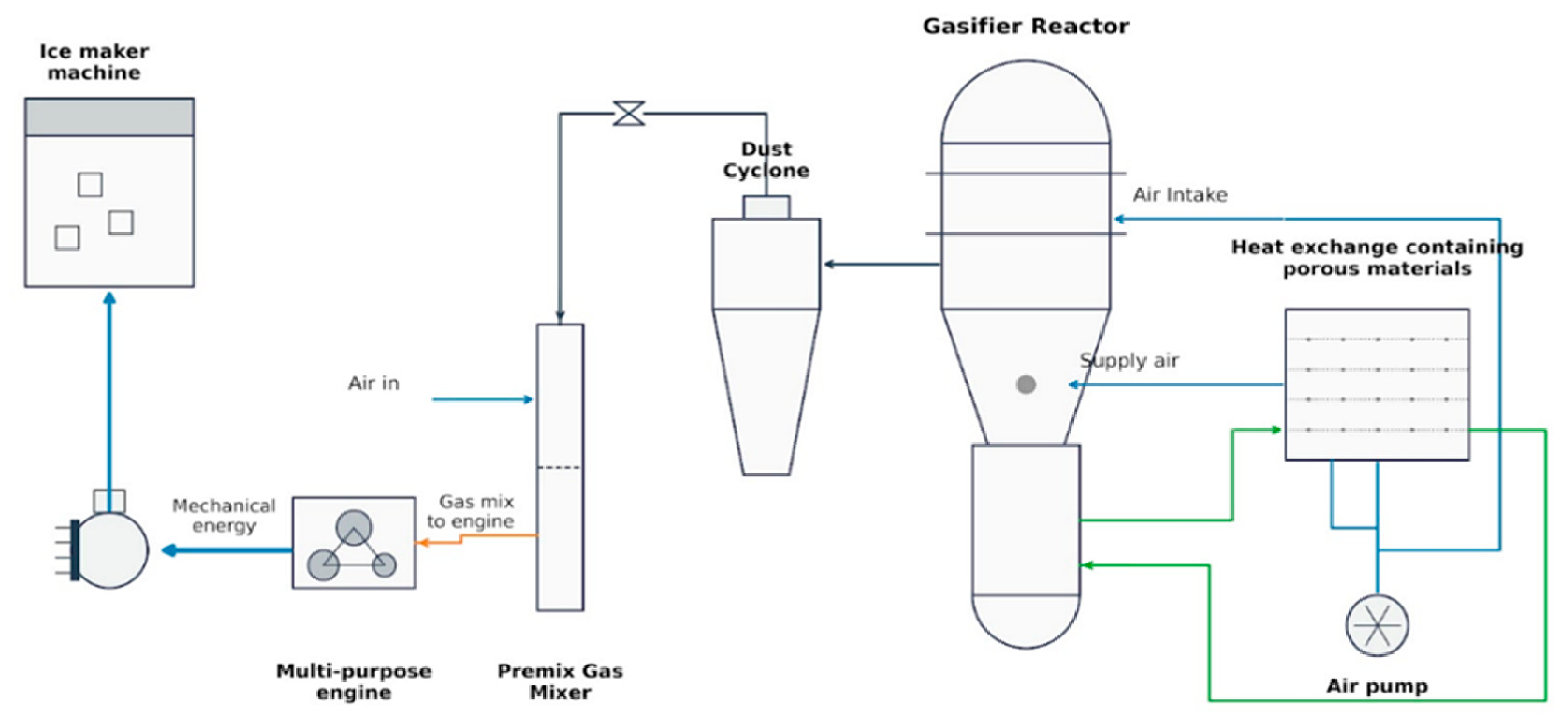
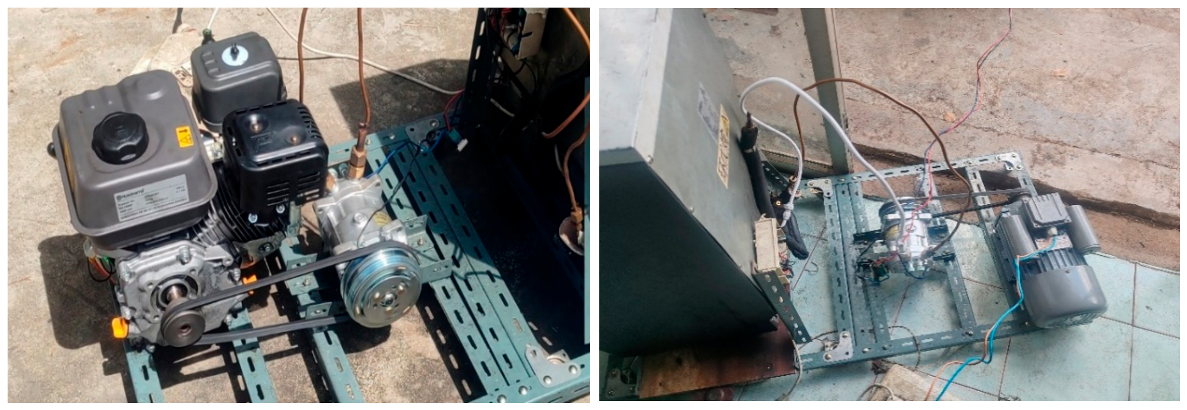
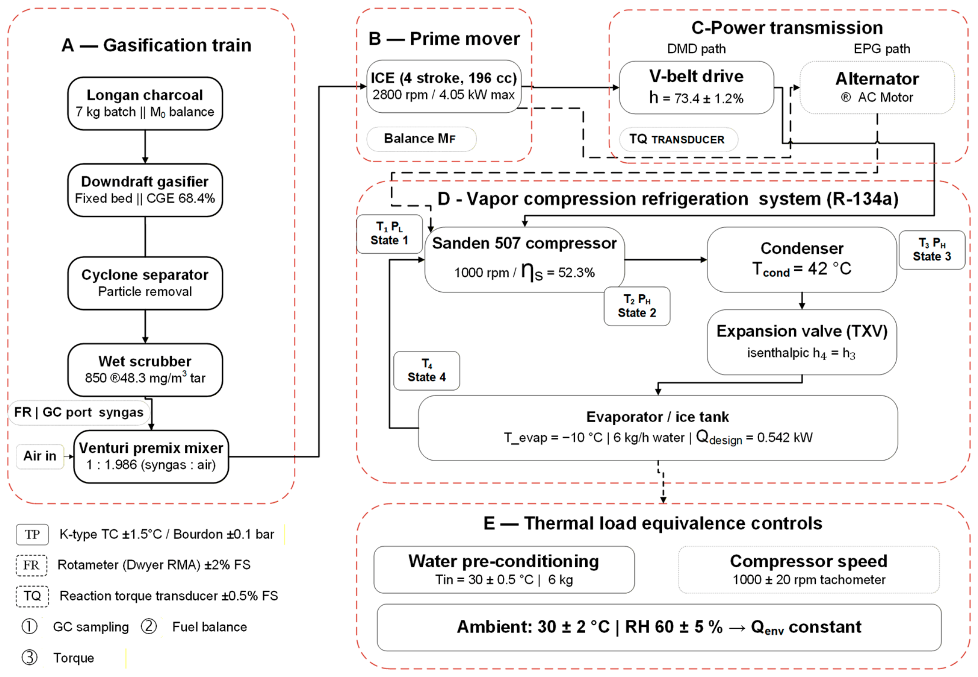
The prototype integrates a downdraft gasifier, a syngas conditioning train, and a VCRS driven via either V-belt (DMD) or a generator-motor set (EPG) (Figure 1 and Figure 2). Uncertainties were evaluated per GUM standards [24]. Due to the lack of a refrigerant flow meter, the cooling capacity (Q_cooling = 0.542 kW) was validated via calorimetric balance, deriving COP from state-point enthalpies: COPR = (h₁ − h₄)/(h₂ − h₁). Although this assumes adiabatic compression, the low shaft-to-refrigerant conversion ratio (η_shaft→ref = 19.6%), defined as the fraction of compressor shaft power that appears as fluid-side compression work (Ẇ_comp,fluid/Ẇ_shaft), the bulk of the shaft input (0.812 kW of the 1.01 kW supplied) is dissipated within the compressor rather than being absorbed by the refrigerant delivered to the condenser; the physical partition of this dissipation is examined quantitatively later in this section. To rigorously resolve the imbalance among cooling capacity, refrigerant mass flow rate, and compressor work input, the total internal shaft-level dissipation—of which mechanical friction is only a minor component (≈0.10 kW at η_mech,comp = 0.90)—must be separated from the refrigerant state-point analysis and assigned exclusively to the mechanical power balance. Specifically, the unrecovered shaft-level dissipation (Ẇ_diss,comp = 0.812 kW)—which is dominated by internal leakage rather than by mechanical friction—is dissipated within the compressor and rejected to the ambient partly through the casing and partly via the recirculated refrigerant, without contributing to the discharge enthalpy of the delivered stream; only the fluid-side irreversibility contributes to the discharge enthalpy (h₂) and to the component exergy destruction (Ex_dest,comp). Neglecting this separation would lead to an overestimation of the compressor’s exergetic efficiency and compromise the overall system exergy balance across the condenser and evaporator boundaries. To ensure thermodynamic consistency across all evaluation boundaries, the shaft-to-refrigerant conversion ratio (η_shaft→ref) is standardized at 19.6% based on the fluid compression work (0.198 kW) relative to the total shaft input (1.01 kW), aligning with the comprehensive shaft power and exergy balance detailed in subsequent sections. Consequently, all internal compressor dissipation—comprising suction-valve leakage, clearance re-expansion, parasitic friction and uninsulated casing heat loss—is lumped into a single shaft-level dissipation term, making the derived COP_R and η_shaft→ref conservative. The calorimetric check bounds the cooling-capacity uncertainty at ±4.8% and the corresponding GUM-propagated COP uncertainty at ±0.23 (±8.4%), both within the tolerance thresholds of ASHRAE Standard 23.1 [25]. Future work requires direct flow metering to decouple compressor heat losses and validate these assumptions. Nevertheless, the current indirect evaluation relies on a rigorous calorimetric energy balance that bounds the system’s cooling-capacity uncertainty to ±4.8%. This margin remains well within the acceptable tolerance thresholds prescribed by ASHRAE Standard 23.1, ensuring that the comparative thermodynamic conclusions drawn in this study remain robust despite the absence of direct mass flow data.

Before the experiments, the HBM T20WN reaction torque transducer (Hottinger Brüel & Kjær, Darmstadt, Germany; 0–50 Nm range, linearity error < ±0.2% FS) was calibrated using standard deadweights in accordance with ISO 6789-1:2017 [26] and mounted directly on the compressor shaft sleeve downstream of the pulley. This architecture isolated internal compressor dissipation from the upstream belt–clutch transmission losses, ensuring that the measured torque represented only the input to the compressor shaft. The transmission pathways are shown in Figure 3. Both configurations used a Husqvarna (Husqvarna Group, Stockholm, Swiden) single-cylinder, four-stroke, 196 cc spark-ignition engine (3600 rpm, 4.05 kW max power, 12.4 Nm max torque). The temperature at key cycle points (T1 to T4) was measured the temperature at key cycle points (T1 to T4) was measured using Omega 5TC-TT-K-30-36 K-type thermocouples (Omega Engineering, Norwalk, CT, USA; ±1.5 °C, IEC 60584-1:2013 Class 2 [27]). Refrigerant-side suction and discharge pressures were measured using WIKA 232.50 calibrated Bourdon tube pressure gauges (WIKA Instrument, Klingenberg, Germany; 0–25 bar range, accuracy class 0.6, ±0.6% of span) in accordance with EN 837-1:1996 [28]. Volumetric syngas flow, fuel consumption, syngas composition, and tar content were measured via a Dwyer RMA-21-SSV calibrated rotameter (Dwyer Instruments, Michigan City, IN, USA; 0–10 m³/h range, ±2% FS) calibrated in accordance with ISO 5167-1:2022 [29], Mettler Toledo XS6002S precision balance (Mettler Toledo, Columbus, OH, USA; 0–6100 g capacity, readability ±0.01 g) calibrated in accordance with OIML R 76-1:2006 [30], gas chromatography using a Shimadzu GC-2014 gas chromatograph equipped with a thermal conductivity detector (TCD) (Shimadzu Corporation, Kyoto, Japan) in accordance with ASTM D1945-14 [31], and Tar content was measured using the gravimetric tar sampling protocol in accordance with CEN/TS 15439:2006 (IEA/BAM protocol) [32], respectively.

Alternator and motor conversion efficiencies were determined from simultaneous measurement of mechanical shaft power (reaction torque transducer) and electrical power (clamp-on power analyzer, ±1.0% of reading) at the steady-state operating point, rather than from manufacturer specifications. Rather than direct measurement, the refrigerant mass flow rate (${\dot{m}}_{ref}$) was quantified indirectly. The cooling capacity (${\dot{Q}}_{cooling}$ = 0.542 kW) was established via the design cooling load (Section 3.1) and validated calorimetrically using the ice formation rate and steady-state bulk water temperature (expanded uncertainty: ±4.8%). System COP values were subsequently derived from thermodynamic state points using measured operating pressures and temperatures, in compliance with ASHRAE Standard 23.1. For future investigations, implementing a Micro Motion ELITE CMF050 Coriolis mass flow meter (Emerson Automation Solutions, Shakopee, MN, USA; ±0.05% of reading)for direct ${\dot{m}}_{ref}$ measurement is recommended in accordance with ISO 10790:2015 [33]. The calculated refrigerant mass flow rate was additionally checked using the compressor displacement-based estimation method. Based on the compressor displacement of 115 cm³/rev at 1000 rpm and a suction density of 9.9 kg/m³ at 1.98 bar and 0 °C, the swept mass flow is 68 kg/h; the enthalpy-derived flow of 0.003566 kg/s (12.84 kg/h) therefore corresponds to an apparent volumetric efficiency of approximately 19%. This low value is attributed to suction-valve leakage, permanent electromagnetic-clutch drag and clearance re-expansion at a fractional load of 7.7–15.5% of rated capacity; the clutch was continuously energized throughout all trials, so the compressor operated without duty cycling, and the measured torque and the derived mass flow rate refer to the same continuous operating basis (Section 4.1). It nonetheless constitutes the principal uncertainty of the present indirect method, and direct Coriolis metering is required to confirm whether the 0.812 kW shaft residual is genuinely frictional or partly reflects an under-estimated cooling capacity. The measurement parameters, instruments, ranges, and accuracies utilized in this study are summarized in

Table 2. Instrumentation summary: measurement parameters, instruments, ranges, and accuracy.

Measured Parameter	Instrument	Range	Accuracy	Location in Schematic
T1–T4 (refrigerant)	K-type TC (IEC 60584 Cl.2)	−40 to 200 °C	±1.5 °C	States 1–4, (Figure 3 and Figure 4)
PL, PH	Bourdon gauge (calibrated)	0–20 bar	±0.1 bar	Comp. suction/discharge
Syngas flow (FR)	Rotameter, Dwyer RMA	0–10 m3/h	±2% FS	Post-scrubber
Fuel mass (Mo, Mf)	Digital balance	0–5 kg	±0.1 g	Charcoal batch
Syngas composition	GC, Shimadzu GC-2014 TCD	—	per GUM prop.	GC port ①
Tar content	IEA/BAM impinger, gravimetric	—	±4.7 mg/m3	Engine inlet
Compressor shaft power	Reaction torque transducer	0–50 Nm	±0.5% FS	Shaft, TQ point ③
Compressor speed	Habotest HT671 (Dongguan Habotest Instrument Technology Co., Ltd., Dongguan, China)	0–3000 rpm	±1 rpm	Compressor pulley

.

A plausibility check on the dissipation pathway supports this interpretation. Rejecting the full 0.812 kW through the compressor casing at the measured shell-to-ambient temperature difference of approximately 45 K would require an effective thermal conductance of hA = 812/45 = 18.0 W/K, whereas the Sanden 507 casing area (0.10–0.20 m²) under combined natural convection and radiation (h ≈ 10–25 W/m²·K) provides only 1.0–5.0 W/K, or 0.05–0.23 kW. The residual therefore cannot be attributed to shell heat loss alone. It is equally inadmissible to assign it to the main refrigerant stream since doing so would raise the discharge enthalpy by 228 kJ/kg and the discharge temperature to approximately 250 °C, in clear contradiction to the measured 75 °C. The remaining physically consistent mechanism is internal suction-valve leakage and clearance re-expansion, in which refrigerant is repeatedly compressed and re-expanded within the compressor and returned to the suction plenum without reaching the condenser. This mechanism dissipates shaft work while contributing neither to the net mass flow nor to the discharge enthalpy of the delivered stream, and it explains why the apparent volumetric efficiency (≈18.9%) and the shaft-to-refrigerant conversion ratio (19.6%) are of the same order: the two are related by η_shaft→ref ≈ η_mech,comp × (Ẇ_comp,fluid/Ẇ_ind), the ratio of delivered to indicated compression duty being 0.198/0.909 = 21.8%, which agrees with the volumetric ratio to within the ≈10% mechanical-loss allowance and the ±4.8% cooling-capacity uncertainty, evaluated through the same enthalpy rise (h₂ − h₁). Independently of this attribution, the evaporator load itself is anchored by the gravimetrically measured ice formation rate of 2 kg/h, which yields a latent duty of 0.186 kW that, together with the sensible and environmental loads of

Table 3. (a) Thermophysical properties, enclosure parameters and resulting refrigeration load terms. (b) Resulting load terms.

(a)
Thermophysical Properties
Parameter	Symbol	Value	Unit	Basis
Specific heat of water (0–30 °C mean)	cp,w	4.19	kJ/kg−1 K−1	ASHRAE Handbook (Fundamentals)
Latent heat of fusion of water at 0 °C	Lf	334.5	kJ/kg−1	ASHRAE Handbook (Fundamentals)
Specific heat of ice (0 to −4 °C mean)	cp,i	2.09	kJ/kg−1 K−1	ASHRAE Handbook (Fundamentals)
Thermal conductivity, polyurethane foam	kins	0.025	W/m−1 K−1	Manufacturer data
Thermal conductivity of ice (Equation (5) only)	kice	2.22	W/m−1 K−1	Not applied (see Note 5)
Batch, temperature and enclosure parameters
Water batch mass processed	mw	6.0 ± 0.05	kg h−1	2.3.1, digital balance
Ice formation rate, steady state	mi	2	kg h−1	Gravimetric, 2.1
Inlet water temperature	Tin	30.0 ± 0.5	°C	K-type, TC
Freezing temperature	Tf	0	°C	—
Final ice temperature	Tice	−4	°C	K-type TC
Ambient/dead-state temperature	Tamb = T0	30 ± 2	°C	2.3
Enclosure temperature difference	ΔTenv	34	K	30 − (−4)
Insulation thickness	tins	35	mm	Measured
Tank shell external surface area	Ashell	0.95	m2	Measured
Wall heat transfer coefficient, as-built	Uwall	0.75	W m−2 K−1	Note 3
Effective coefficient incl. heat bridges	Ueff	2.2	W m−2 K−1	${\dot{Q}}_{env}$/(Ashell × ΔTenv)
Design margin	—	15	%	Component-sizing allowance
(b)
Load Term	Expression	kJ h−1	kW	% of  ${\dot{\mathit{Q}}}_{\mathit{t}\mathit{o}\mathit{t}\mathit{a}\mathit{l}}$
Sensible cooling of water, 30 → 0 °C	mw × cp,w × ΔT (6.0 × 4.19 × 30)	754.2	0.2095	44.5
Latent heat of solidification at 0 °C	mi × Lf (2.0 × 334.5)	669	0.1858	39.4
Sensible cooling of ice, 0 → −4 °C	mi × cp,I × ΔT (2.0 × 2.09 × 4)	16.7	0.0046	1
Conduction through insulated shell, $\dot{\mathrm{Q}}$wall	Uwall × Ashell × ΔTenv × 3.6 (0.75 × 0.95 × 34 × 3.6)	87.2	0.0242	−5.1
Parasitic heat bridges, $\dot{\mathrm{Q}}$bridge	Estimated allowance (Note 4)	168.8	0.0469	−10
Environmental heat gain, $\dot{\mathrm{Q}}$env	$\dot{\mathrm{Q}}$wall + $\dot{\mathrm{Q}}$bridge	256	0.0711	15.1
Total cooling load, $\dot{\mathrm{Q}}$total	Σ$\dot{\mathrm{Q}}$ (four additive terms)	1695.90	0.4711	100
Design margin (15%)	0.15 × $\dot{\mathrm{Q}}$total	254.4	0.0707	—
Design cooling capacity, $\dot{\mathrm{Q}}$design	1.15 × $\dot{\mathrm{Q}}$total	1950.30	0.542	—

Note 1: Load basis. All terms are evaluated on a quasi-steady hourly basis (Section 2.4). Of the 6.0 kg h⁻¹ processed, 2.0 kg h⁻¹ is converted to ice at −4 °C, while the remaining 4.0 kg h⁻¹ is sensibly cooled to 0 °C only; the water sensible term therefore applies to the full 6.0 kg h⁻¹, whereas the latent and ice-sensible terms apply to the 2.0 kg h⁻¹ ice throughput alone. Rows marked are sub-items of $\dot{Q}$_env and are not separately additive in the total. Note 2: Closure. The four additive terms sum to 1695.9 kJ h⁻¹; application of the 15% design margin returns $\dot{Q}$_design = 1950.3 kJ h⁻¹ = 0.542 kW identically, which is the single cooling-capacity value carried through every energy and exergy balance in this work. The latent term of 0.186 kW quoted in Section 2.1 is the second row of this table, so the design capacity is anchored on the gravimetrically measured ice formation rate and the measured water batch mass, independently of any refrigerant state point. Note 3: Wall conductance. The conduction-only value implied by the insulation alone is ki_ns/t_ins = 0.025/0.035 = 0.71 W m⁻² K⁻¹. The as-built value of 0.75 W m⁻² K⁻¹ adopted here includes a 5% allowance for local insulation compression at mechanical fixings and for seam gaps. Internal and external surface film resistances are neglected, which is conservative in that it overestimates the conductive load. Note 4: Heat-bridge term. $\dot{Q}$_bridge is an engineering allowance covering the structural steel mounting frame, the copper refrigerant piping penetrations (≈3 mm OD) and the insulated lid perimeter seal; it was not measured directly and constitutes the principal uncertainty of the load calculation. The resulting ratio  $\dot{Q}$_env/$\dot{Q}$_wall = 2.94 lies within the 1.5–4× heat-bridge penalty range reported for prototype-grade enclosures with structural penetrations. Guarded-hot-box or transient calorimetric characterization of the tank is recommended to replace this allowance with a measured value. Note 5: Ice conductivity. k_ice is tabulated for completeness with the ice-layer resistance of Equation (5) and is not applied in the quasi-steady framework adopted in this work (Section 2.4). Note 6: Full-cycle cross-check. Freezing the entire 6.0 kg batch to −4 °C requires 6.0 × (4.19 × 30 + 334.5 + 2.09 × 4) = 2811 kJ, i.e., 1.44 h at the design capacity of 0.542 kW, consistent with the freezing-cycle duration used in Section 3.2.

, reproduces the 0.542 kW design capacity without recourse to refrigerant state points. The refrigerant-side balance is therefore closed on a directly measured basis, and the pending question concerns only the internal partition of the 0.812 kW shaft residual, not the magnitude of the cooling capacity.

2.2. Gasifier Design and Syngas Conditioning

To minimize tar concentration, a downdraft fixed-bed gasifier [34,35,36] was selected, operating with a 20% safety margin to ensure consistent fuel delivery [15]. In the reduction zone, the thermochemical conversion was primarily driven by endothermic Boudouard and water–gas reactions. At an engine speed of 2800 rpm, the swept volume of the 196 cc engine is 16.47 m³/h; applying a volumetric efficiency of 0.80, typical of naturally aspirated small SI engines, on producer gas gives an aspirated mixture throughput of 13.2 m³/h. With the premix ratio of 1:1.986 (syngas-to-air), the corresponding syngas demand at the intake is 4.42 m³/h, establishing a minimum gasifier design capacity of 8.5 m³/h after the 20% safety margin and part-load allowance.

At the operating point, the entire gasifier output is aspirated by the engine, with no venting, so that the full syngas chemical energy of Section 2.6 is delivered to the ICE. The orifice-derived volumetric readings (syngas 7.63 Nm³/h; air 15.15 m³/h) correspond to a mixture throughput larger than the swept volume of the 196 cc engine at 2800 rpm, indicating that these anemometric readings represent center-line rather than area-averaged velocities; they are therefore reported as design-verification estimates only, whereas the energy balance of Section 2.6 is anchored on the gravimetrically measured charcoal consumption together with the measured cold gas efficiency, and cross-checked by the gravimetric syngas mass flow. Experimentally, the integrated Venturi mixer delivered a measured syngas flow of 7.63 Nm³/h (via a 15-mm orifice at 12.0 m/s), reported at normal conditions (0 °C, 101.325 kPa) consistent with the gas-chromatography basis. Furthermore, to satisfy the <100 mg/m³ threshold required for stable spark-ignition operation [37], the syngas conditioning train—consisting of a cyclone separator, a packed-bed wet scrubber (2 L/min), and a moisture separator—effectively reduced tar levels from approximately 850 mg/m³ to 48.3 ± 4.7 mg/m³ (as verified by the gravimetric IEA/BAM protocol):

$$C+{CO}_2\leftrightharpoons 2CO\left(+172{\displaystyle \frac{\mathrm{k}\mathrm{J}}{\mathrm{m}\mathrm{o}\mathrm{l}}}\right)$$

$$C+H_{2}O\leftrightharpoons CO+H_2\left(+131{\displaystyle \frac{\mathrm{k}\mathrm{J}}{\mathrm{m}\mathrm{o}\mathrm{l}}}\right)$$

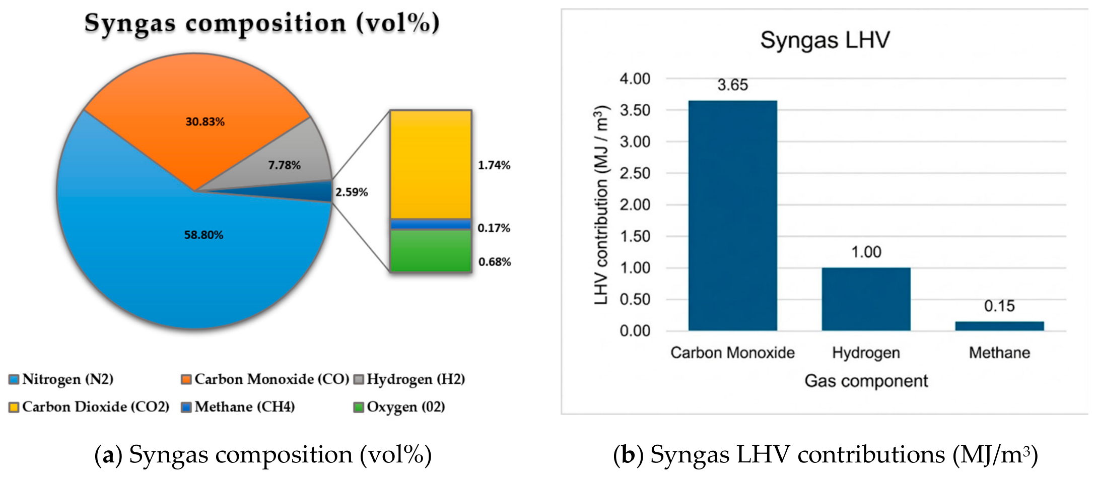
Given the utilization of carbonized charcoal as the primary feedstock, the substantial fractions of CO (30.83%) and H₂ (7.78%) in the product gas indicate that fixed-carbon reduction at temperatures in the reduction zone exceeding 950 °C was the dominant mechanism, rather than volatile cracking. This highly efficient conversion yielded a cold gas efficiency (CGE) of approximately 68.4% (

Table 4. Characterized properties of longan wood charcoal and its derived syngas.

Component/Property	Value (Mean ± SD)	Unit
Nitrogen (N2)	58.80 ± 0.42	vol%
Carbon Monoxide (CO)	30.83 ± 0.68	vol%
Hydrogen (H2)	7.78 ± 0.31	vol%
Carbon Dioxide (CO2)	1.74 ± 0.08	vol%
Methane (CH4)	0.17 ± 0.02	vol%
Oxygen (O2)	0.68 ± 0.05	vol%
Apparent Molecular Weight	26.06 ± 0.12	g/mol
Lower Heating Value (LHV)—volumetric	4.79 ± 0.15	MJ/m3
Feedstock (longan charcoal) LHV, gravimetric [38,39]	29.0 ± 0.4	MJ/kg
Feedstock moisture (as-received)	5.0 ± 0.5	wt%
Feedstock fixed carbon (as-received)	85.8 ± 1.2	wt%
Syngas LHV, gravimetric	4.12	MJ/kg
Tar Content (engine inlet, post-scrubber)	48.3 ± 4.7	mg/m3
Cold Gas Efficiency (CGE), measured	68.4 ± 2.1	%

), optimizing the gaseous fuel mixture to support stable laminar flame propagation during subsequent engine combustion.

2.3. Experimental Protocol and Statistical Analysis

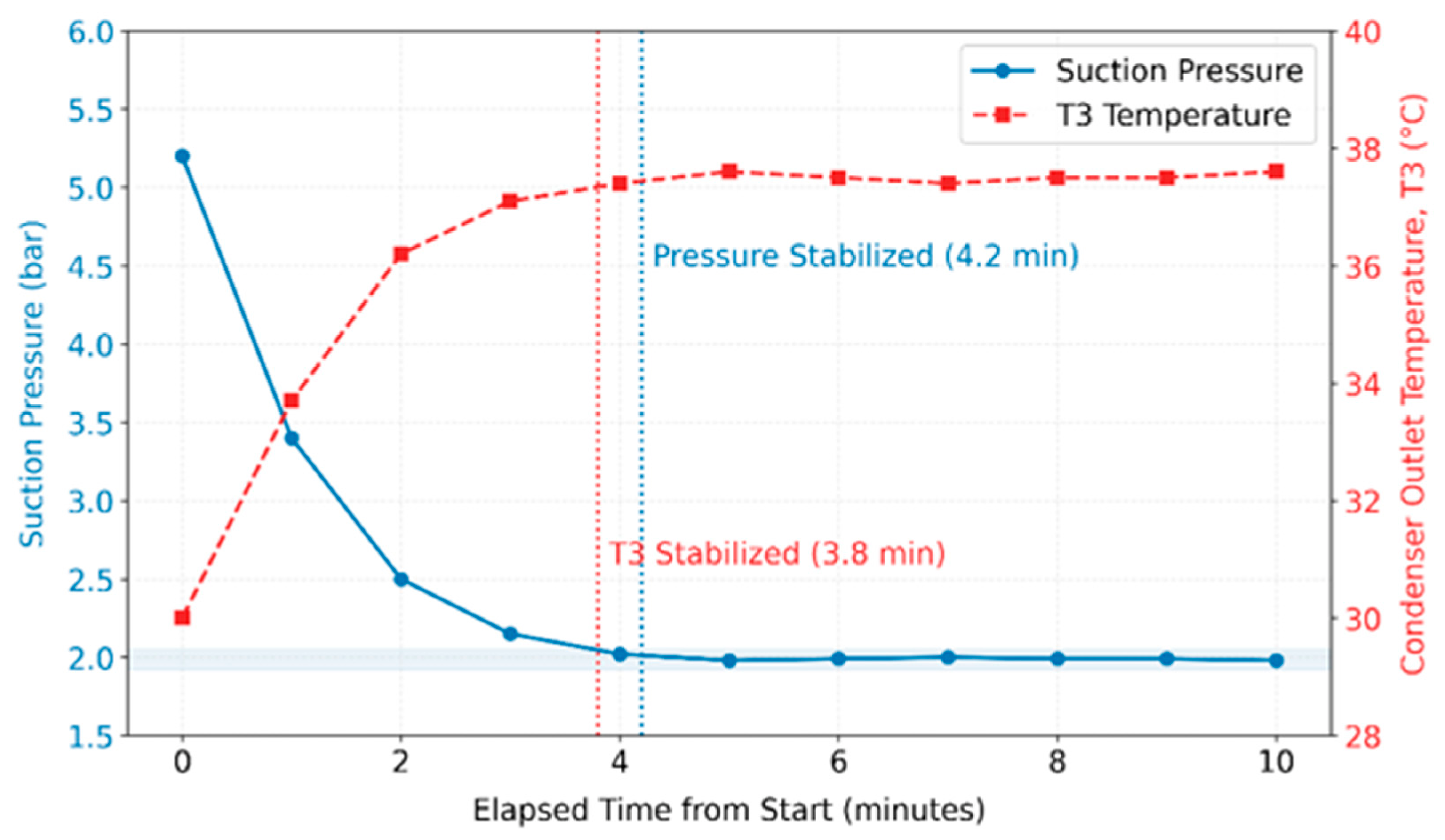
All experiments were conducted under strictly controlled ambient conditions (30 ± 2 °C, 60 ± 5% RH). To guarantee accurate steady-state COP evaluations, data acquisition was initiated only after a 15 min ICE warm-up and subsequent VCRS pressure stabilization (deviation < 0.05 bar over 5 min), deliberately omitting the initial 4 min transient phase. A randomized block design (n = 5 per setup, 10 trials total) was implemented to mitigate temporal confounding between the DMD and EPG configurations. The adequacy of this sample size was confirmed via an a priori power analysis (G_Power: two-tailed paired t-test, α = 0.05, 1 − β = 0.80, effect size d = 2.0, minimum n = 4), achieving a post hoc power > 0.90 for the observed effect size (Cohen’s d = 32.1, SDdiff = 9.23 g/h; Supplementary Table S1). This effect size is unusually large owing to the very small pooled standard deviation for this comparison, and should therefore be interpreted qualitatively rather than by conventional d thresholds. A two-tailed paired-samples t-test (α = 0.05) evaluated the null hypotheses regarding differences in mean fuel consumption and COPR. All statistical operations were executed using Python (SciPy v1.10.1), with results presented as mean ± standard deviation (SD) alongside 95% confidence intervals.

2.3.1. Thermal Load Equivalence and Control Strategy

Thermal load equivalence across all 10 trials was maintained using three control variables: (i) an ice tank with 6.0 ± 0.05 kg water at 30.0 ± 0.5 °C; (ii) a fixed compressor shaft speed of 1000 ± 20 rpm with equivalent torque (9.64 ± 0.15 Nm); and (iii) ambient conditions at 30 ± 2 °C and 60 ± 5% RH. This yielded a constant cooling load (Q_design = 0.542 kW) and environmental heat gain (Q_env = 256 kJ/h), verified post hoc by a mean evaporation pressure of 1.98 ± 0.04 bar (T_sat = −10 °C). Additionally, the belt–clutch transmission efficiency was evaluated as η_belt = Ẇ_shaft/Ẇ_brake = 1.01/1.38 = 73.2%. This value should therefore be interpreted as an apparent transmission efficiency under the present measurement boundary rather than the intrinsic efficiency of the V-belt itself. The deviation from conventional V-belt efficiency mainly reflects the combined effects of clutch drag, pulley-side losses, and uncertainty in the inferred engine brake power. Because the reaction torque transducer is mounted on the compressor shaft downstream of the pulley, only the downstream term is measured directly; the upstream engine brake power is obtained from the syngas chemical energy input and the brake thermal efficiency of the engine, so that η_belt is an inferred rather than a directly metered quantity and inherits the uncertainty of both terms (combined standard uncertainty ±4.1 percentage points, k = 1). Since shaft work is pure exergy, the energetic and exergetic transmission efficiencies are numerically identical, and the single value 73.2% is used in both the system-level energy balance and the component-level exergy analysis discussed in subsequent sections. This figure lies below the 95–98% typically quoted for correctly tensioned and aligned V-belt drives operating near their design load, and the physical basis for the discrepancy is examined in Section 4.1.

2.3.2. Sequential Empirical Methodology

Phase 1—Pre-trial preparation: Record initial charcoal mass (M₀), fill the reservoir with 6.0 ± 0.05 kg of water (T_in = 30 ± 0.5 °C), and maintain a 2 L/min wet scrubber supply. Set compressor speed to 1000 ± 20 rpm. Verify AC motor connections for EPG and inspect V-belt tension for DMD using the deflection method [40]. The inferred belt–clutch transmission efficiency was low (73.2%), which is attributed to torque pulsation from the single-cylinder engine, pulley misalignment, permanent electromagnetic-clutch drag and idler friction rather than to gross belt slip, since the measured speed ratio matches the geometric pulley ratio to within ±2% (Section 4.1); a synchronous belt drive is recommended to eliminate the tension-dependent bending-hysteresis loss and to provide a positive speed ratio.

Phase 2—Gasifier initiation and stabilization: Initiate the gasifier and stabilize the syngas flow rate at 7.63 ± 0.2 m³/h (the measured steady-state value) (requiring ≥15 min engine preconditioning). Start the engine and engage the refrigeration circuit. Maintain operation until dual equilibrium criteria are met: (a) suction pressure deviation < 0.05 bar and (b) T₁ deviation < 0.5 °C, both over a 5 min window.

Phase 3—Data acquisition: Log T₁, T₂, T₃, T₄, P_L, P_H, and syngas flow rate every 60 s. A minimum 10 min steady-state period was required before batch depletion; otherwise, the trial was discarded and re-executed. Record elapsed time (t_elapsed) and weigh final charcoal mass (M_f) immediately upon batch depletion to calculate fuel consumption rate: (M₀ − M_f)/t_elapsed.

Phase 4—Configuration changeover: Allow a ≥30 min cool-down period before switching configurations, and perform a torque transducer zero-calibration check prior to the next trial.

2.4. Refrigeration Load Calculation

The total cooling load Q_total comprises sensible heat removal from the water, latent heat of solidification, sensible heat removal from ice, and environmental heat gain through the insulated storage vessel:

$$Q_{total}=Q_{water}+Q_{ice}+Q_{env}$$

(1)

$$Q_{water}={\dot{m}}_{water}\times C_{p,w}\times {\Delta T}_w$$

(2)

$$Q_{ice}=\left({\dot{m}}_{ice}\times L_f\right)+\left[({{\dot{m}}_{ice}\times C}_{p,i}\times \left|{∆T}_i\right|)\right]$$

(3)

$$Q_{env}={U\times A}_{shell}\times {∆T}_{env}$$

(4)

The environmental heat gain, Q_env, was evaluated as the aggregate of two physically distinct heat transfer pathways across the insulated tank boundary. The first pathway is conductive heat transfer through the 35 mm polyurethane foam shell (k = 0.025 W/m·K), governed by Equation (4) and evaluated at the steady-state temperature difference ΔT = 30 − (−4) = 34 K, yielding Q_wall = 0.75 × 0.95 × 34 × 3.6 = 87.2 kJ/h. The second pathway encompasses parasitic heat bridges through the structural steel mounting frame, copper refrigerant piping penetrations (≈3 mm OD), and the insulated lid perimeter seal, contributing an estimated Q_bridge = 168.8 kJ/h. The combined environmental load Q_env = Q_wall + Q_bridge = 87.2 + 168.8 = 256.0 kJ/h, equivalent to an effective system-level heat transfer coefficient of U_eff = 2.20 W/(m²·K), is consistent with published heat bridge penalty factors of 1.5–4× the insulation-only conductance for prototype-grade enclosures with structural penetrations. The first and second terms in the equation represent the latent heat of solidification at 0 °C and the sensible cooling of ice to −4 °C, respectively. An ice production rate of 2 kg/h represents the steady-state throughput, while the remaining 4 kg/h undergoes sensible cooling based on the quasi-steady-state protocol outlined in Section 2.3. The thermodynamic parameters used to determine the specific cooling loads (Q_water, Q_ice) and the environmental heat infiltration (Q_env) are detailed in Table 3. Because every entry of Table 3 is either a tabulated thermophysical property or a directly measured mass, temperature or area, the design cooling capacity of 0.542 kW is established without recourse to refrigerant state points or to the refrigerant mass flow rate; the state-point analysis of Section 2.5 is therefore a consistency check on an independently anchored load rather than its source.

By aggregating these loads and applying a 15% design margin, the total design cooling capacity (Q_design) is established at 1950.3 kJ/h (0.542 kW), serving as the baseline for component sizing. While ice formation is inherently a transient process characterized by time-dependent thermal resistance from ice-layer growth, this study utilizes a quasi-steady-state framework. To mitigate transient effects, data collection commenced only after the system reached complete pressure stabilization (Section 2.3.2), ensuring that the primary phase of ice-layer accumulation was completed prior to performance evaluation.

$$R_{ice}={\displaystyle \frac{\ln \left(r_o/r_i\right)}{2\pi k_{ice}L}}$$

(5)

This progressive ice accumulation suppresses the evaporating temperature and alters the compressor’s volumetric efficiency throughout the freezing cycle. Although the time-dependent conductive resistance of the ice layer (Rice, Equation (5)) is a non-trivial factor for transient performance modeling, it was not explicitly incorporated into the current quasi-steady-state framework. Transient analyses of domestic vapor compression systems have demonstrated that both refrigerant charge level and ambient temperature fluctuations significantly alter system pressure profiles and COP during start-up and load-change periods [41]; future work employing such transient thermal simulations could accurately quantify the impact of Rice on COP degradation [42]. Regardless, because both the DMD and EPG configurations demonstrated statistically identical ice growth rates and evaporating pressure profiles under a controlled load, the relative comparison of their thermodynamic and fuel economy performance under the quasi-steady-state assumption remains rigorously valid.

2.5. Vapor Compression Refrigeration Cycle Analysis

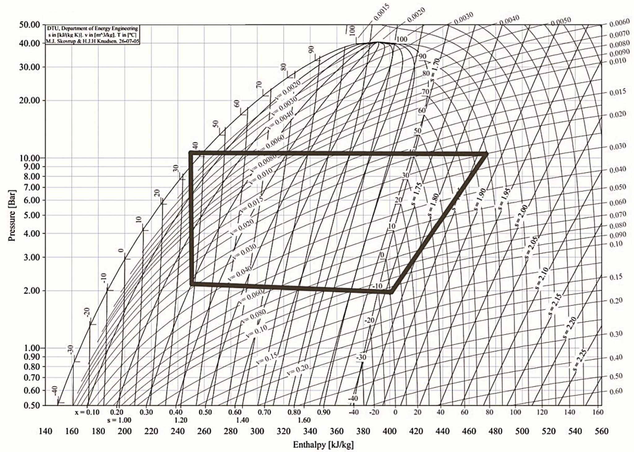
The VCRS operates on R-134a. Thermodynamic state points were determined at four key locations: compressor suction (State 1), compressor discharge (State 2), condenser exit (State 3), and expansion device inlet (State 4 = State 3, isenthalpic expansion). Based on the measured operating conditions—suction pressure P₁ = 1.98 bar (T_sat ≈ −10 °C), discharge pressure P₂ = 11.01 bar (T_sat ≈ 42 °C), superheat of 10 K at State 1 (T₁ = 0 °C), actual discharge temperature T₂ = 75 °C, and subcooling of 5 K at State 3 (T₃ = 37 °C)—enthalpies were extracted from NIST REFPROP data for R-134a. The measured state point conditions and corresponding enthalpy values are summarized in Table 5, and the complete thermodynamic cycle is represented on the pressure-enthalpy (P-h) diagram in Figure 4.

Table 5. Measured thermodynamic state points of the R-134a vapor compression cycle.

State	Description	T (°C)	P (bar)	h (kJ/kg)	Note
1	Compressor Suction	0	1.98	401	10 K superheat
2s	Isentropic Discharge	—	11.01	430	Ideal compression
2	Actual Discharge	75	11.01	456.5	ηis = 0.523
3	Condenser Exit (liquid)	37	11.01	249	5 K subcooling
4	Expansion Valve Exit	−10	1.98	249	h4 = h3 (isenthalpic)
COPR		2.74 ± 0.23			Qevap/Wcomp,fluid
${\dot{m}}_{ref }$ (kg/s|kg/h)		0.003566/12.84			${\dot{Q}}_{cooling }$/(h1 − h4)
${\dot{W}}_{comp, fluid }$ (kW)		0.198			${\dot{m}}_{ref}$(h2 − h1)
${\dot{Q}}_{cond }$ (kW) (1)		0.740			${\dot{Q}}_{evap}$ + ${\dot{W}}_{comp,fluid }$
${\dot{Q}}_{cond }$ (kW) (2)		0.740			${\dot{m}}_{ref}$(h2 − h3)
Error		<0.001 kW

Note: The discharge temperature of 75 °C is attributed to the non-isentropic fluid compression (η_is = 52.3%), consistent with the refrigerant energy balance in Section 2.6; the shaft-level dissipation (Ẇ_diss,comp = 0.812 kW), of which only ≈0.10 kW is mechanical friction, is dissipated internally within the compressor and does not raise h₂ (Section 2.1). The reported uncertainty (±0.23) is the GUM-propagated value for a single representative cycle (Equation (9)); it is not the experimental standard deviation (±0.15/±0.13). The condenser duty is obtained independently from the refrigerant-circuit balance ($\dot{Q}$_evap + Ẇ_comp,fluid), where the residual error remains below 0.001 kW, and from the enthalpy difference across the condenser (ṁ_ref(h₂ − h₃)); the two routes agree to within 0.001 kW, confirming mutual consistency of the cooling capacity, the enthalpy-derived mass flow rate and the fluid-side compression work.

Table 5. Measured thermodynamic state points of the R-134a vapor compression cycle.

State	Description	T (°C)	P (bar)	h (kJ/kg)	Note
1	Compressor Suction	0	1.98	401	10 K superheat
2s	Isentropic Discharge	—	11.01	430	Ideal compression
2	Actual Discharge	75	11.01	456.5	ηis = 0.523
3	Condenser Exit (liquid)	37	11.01	249	5 K subcooling
4	Expansion Valve Exit	−10	1.98	249	h4 = h3 (isenthalpic)
COPR		2.74 ± 0.23			Qevap/Wcomp,fluid
${\dot{m}}_{ref }$ (kg/s|kg/h)		0.003566/12.84			${\dot{Q}}_{cooling }$/(h1 − h4)
${\dot{W}}_{comp, fluid }$ (kW)		0.198			${\dot{m}}_{ref}$(h2 − h1)
${\dot{Q}}_{cond }$ (kW) (1)		0.740			${\dot{Q}}_{evap}$ + ${\dot{W}}_{comp,fluid }$
${\dot{Q}}_{cond }$ (kW) (2)		0.740			${\dot{m}}_{ref}$(h2 − h3)
Error		<0.001 kW

Note: The discharge temperature of 75 °C is attributed to the non-isentropic fluid compression (η_is = 52.3%), consistent with the refrigerant energy balance in Section 2.6; the shaft-level dissipation (Ẇ_diss,comp = 0.812 kW), of which only ≈0.10 kW is mechanical friction, is dissipated internally within the compressor and does not raise h₂ (Section 2.1). The reported uncertainty (±0.23) is the GUM-propagated value for a single representative cycle (Equation (9)); it is not the experimental standard deviation (±0.15/±0.13). The condenser duty is obtained independently from the refrigerant-circuit balance ($\dot{Q}$_evap + Ẇ_comp,fluid), where the residual error remains below 0.001 kW, and from the enthalpy difference across the condenser (ṁ_ref(h₂ − h₃)); the two routes agree to within 0.001 kW, confirming mutual consistency of the cooling capacity, the enthalpy-derived mass flow rate and the fluid-side compression work.

Figure 4. Pressure–enthalpy (log p-h) diagram for refrigerant R134a. The diagram was generated using CoolPack simulation software v1.5 [43] and is based on thermodynamic property correlations from Wilson and Basu [44]. Adapted with attribution from CoolPack software, Department of Energy Engineering, Technical University of Denmark (DTU), 2005.

Figure 4. Pressure–enthalpy (log p-h) diagram for refrigerant R134a. The diagram was generated using CoolPack simulation software v1.5 [43] and is based on thermodynamic property correlations from Wilson and Basu [44]. Adapted with attribution from CoolPack software, Department of Energy Engineering, Technical University of Denmark (DTU), 2005.

State 1 (compressor suction, h₁ = 401 kJ/kg at 1.98 bar) and State 2 (actual discharge, h₂ = 456.5 kJ/kg at 11.01 bar and 75 °C) define the compression work input W_comp, while the horizontal distance between State 4 and State 1 on the evaporation line in Figure 4 represents the useful refrigeration effect Q_evap. The isentropic efficiency of the compressor was determined directly from the measured state-point enthalpies as

$${\eta }_{is}={\displaystyle \frac{h_{2s}-h_1}{h_2-h_1}}={\displaystyle \frac{430-401}{456.5-401}}={\displaystyle \frac{29.0}{55.5}}=0.523$$

(6)

where h₂s = 430 kJ/kg is the isentropic discharge enthalpy at P₂ = 11.01 bar for the same entropy as State 1, extracted from NIST REFPROP. This experimentally derived value—rather than an assumed literature value—confirms the compressor’s measured performance under syngas-driven operating conditions. The relatively low isentropic efficiency is attributed to the compressor operation under severe fractional-load conditions (7.7–15.5% of rated capacity), where increased leakage, clearance re-expansion, and intermittent clutch losses significantly reduce effective compression performance.

To ensure rigorous thermodynamic interpretation, performance metrics are normalized across four explicitly nested system boundaries: the refrigerant control volume (COP_R), the compressor shaft (COP_shaft), the syngas delivered to the engine inlet (η_syngas = 5.34%), and the primary biomass feedstock (η_sys = 3.66% and ε_sys = 0.44%). Only the last of these is described as a system-level efficiency in this work; the syngas-referenced value is reported solely to permit comparison with studies that draw their boundary at the gasifier outlet. The refrigeration cycle performance (COP_R) is defined as the ratio of the evaporator cooling load to the actual fluid-side compression work (W_comp,fluid), evaluated strictly within the refrigerant control volume:

$${COP}_R={\displaystyle \frac{Q_{\mathrm{e}\mathrm{v}\mathrm{e}\mathrm{p}}}{W_{\mathrm{c}\mathrm{o}\mathrm{m}\mathrm{p}}}}={\displaystyle \frac{h_1- h_4}{h_2- h_1}}={\displaystyle \frac{152}{55.5}}=2.74$$

(7)

The biomass-referenced system COP evaluates the cooling output relative to the chemical energy input of the original biomass feedstock, including the gasification conversion step. Finally, the exergetic efficiency is normalized by the total chemical exergy input of the biomass (${Ex}_{evap}/{\dot{Ex}}_{biomass}$) to quantify the cumulative destruction of work potential throughout the entire conversion chain, where Q_evap = h₁ − h₄ = 152 kJ/kg is the enthalpy change across the evaporator. The calculated refrigerant mass flow rate was subsequently checked against the compressor displacement and operating speed to ensure physical consistency with the measured compressor operating condition. Although the indirect determination introduces uncertainty in the absolute refrigerant flow rate, the agreement between evaporator-side cooling capacity, compressor fluid work, and condenser heat rejection demonstrates that the derived mass flow rate satisfies the First-Law energy conservation requirement within the measurement uncertainty. It is noted that the isentropic efficiency of 52.3% reflects the fidelity of the refrigerant compression process between States 1 and 2, evaluated solely from measured refrigerant-side state points via NIST REFPROP. Therefore, η_is = 52.3% and η_is,shaft = 10.2% should not be directly compared because the former is defined within the refrigerant control volume using fluid compression work, whereas the latter includes all upstream shaft-level losses.

The corresponding shaft-referred coefficient of performance, COP_shaft = ${\dot{Q}}_{cooling}/{\dot{W}}_{shaft}$ = 0.542/1.01 = 0.537, is reported separately in Section 3.2, and the biomass-referenced First-Law system efficiency is η_sys = 0.542/14.82 = 3.66%. This value reflects a rigorous thermodynamic accounting of the measured 75 °C discharge temperature, which arises solely from the non-isentropic fluid compression (η_is = 52.3%) and not from the shaft-level dissipation; the latter are dissipated within the compressor as internal suction-valve leakage, clearance re-expansion and parasitic friction and are rejected to the ambient partly through the casing and partly via the recirculated refrigerant, without contributing to the discharge enthalpy of the delivered stream, as detailed in Section 2.1 and Section 2.6. Although this COPR is constrained by the non-isentropic compression characteristics at the compressor discharge, the DMD configuration remains highly competitive for small-scale, off-grid biomass-powered applications. By effectively bypassing the conversion losses associated with electrical power generation, the DMD system justifies its performance despite these compression irreversibilities.

Furthermore, it is important to note that the recorded COP_R of 2.74 does not account for the substantial shaft-level dissipation (Ẇ_diss,comp = 0.812 kW). This dissipated power is rejected within the compressor as internal suction-valve leakage, clearance re-expansion and parasitic friction and is rejected to the ambient partly through the casing and partly via the recirculated refrigerant (Section 2.1); it is therefore excluded from the refrigerant-circuit energy balance (Q_cond = Q_evap + W_comp,fluid = 0.740 kW) and consequently does not appear as an elevation of the discharge enthalpy. The measured discharge temperature (T₂ = 75 °C) instead reflects the non-isentropic fluid compression (η_is = 52.3%), for which the actual enthalpy rise (55.5 kJ/kg) exceeds the isentropic value (29 kJ/kg). To enhance the system’s thermal efficiency in future iterations, optimization strategies should prioritize increasing the subcooling degree at the condenser outlet; by reducing the liquid enthalpy at State 3, the refrigeration capacity (Q_evap = h₁ − h₄) can be expanded, potentially elevating the COP_R to values exceeding 3.5 without requiring changes to the primary mechanical configuration. Consequently, the compressor isentropic efficiency of 52.3%, derived from state-point enthalpies, supersedes manufacturer-rated values and ensures thermodynamic closure across the refrigerant and mechanical boundaries; the shaft-referred metric is reported separately in Section 3.2 and discussed in Section 4.1.

The shaft-referred isentropic efficiency references the isentropic compression work to the total shaft power input rather than to the fluid-side enthalpy rise and is defined by Equation (8):

$${\eta }_{is,shaft}={\displaystyle \frac{{\dot{m}}_{ref}(h_{2s}-h_1)}{W_{shaft}}}={\eta }_{is}\times {\eta }_m$$

(8)

Evaluated directly from the unrounded state-point and mass-flow values, η_is,shaft = ṁ_ref(h₂s − h₁)/Ẇ_shaft = 0.003566 × (430 − 401)/1.01 = 0.1034/1.01 = 10.2%. Because η_is = ṁ_ref(h₂s − h₁)/Ẇ_comp,fluid and η_shaft→ref = Ẇ_comp,fluid/Ẇ_shaft, the relation η_is,shaft = η_is × η_shaft→ref is an exact algebraic identity rather than an approximation; the product of the rounded values quoted in the text (0.523 × 0.196) returns 10.3%, the 0.1-percentage-point difference being a rounding artefact only. As an independent check, η_is,shaft = η_is × (COP_shaft/COP_R) = 0.523 × (0.537/2.74) = 10.2% since COP_shaft/COP_R is identically η_shaft→ref. The single value adopted throughout this work is therefore η_is,shaft = 10.2%; no alternative shaft-referred isentropic efficiency is reported anywhere in this study. Definitive separation of the shaft-level dissipation from any residual under-estimation of the cooling capacity requires calorimetric shell heat-loss measurement together with direct refrigerant flow metering and is recommended for future work (Section 4.4). The uncertainty propagation for the coefficient of performance (COP = 2.74 ± 0.23) was rigorously evaluated in accordance with the Guide to the Expression of Uncertainty in Measurement (GUM). The enthalpy uncertainties (δh₁ = δh₂ = ±1.35 kJ/kg, δh₃ = δh₄ = ±1.95 kJ/kg) were derived from a temperature measurement uncertainty of ±1.5 °C by utilizing a specific heat capacity (cp) value of 1.02 kJ/kg (at 1.98 bar, 0 °C) for R-134a under the corresponding suction and discharge pressures. The full error propagation equation governing the refrigeration cycle is expressed as follows:

$${\delta }_{COP}=\sqrt{{\left({\displaystyle \frac{\mathsf{\partial }COP}{\mathsf{\partial }{h}_1}}\delta h_1\right)}^2+{\left({\displaystyle \frac{\mathsf{\partial }COP}{\mathsf{\partial }{h}_2}}\delta h_2\right)}^2+\cdots +{\left({\displaystyle \frac{\mathsf{\partial }COP}{\mathsf{\partial }{h}_n}}\delta h_n\right)}^2}$$

(9)

where the partial derivatives represent the mathematical sensitivity of COP to individual state-point enthalpies. Evaluated numerically for the measured operating conditions, the dominant uncertainty contributions arise from h₁ (∂COP/∂h₁ = (h₂ − h₄)/(h₂ − h₁)² = 4.37 kg/kJ) and h₂ (∂COP/∂h₂ = −(h₁ − h₄)/(h₂ − h₁)² = −1.16 kg/kJ), yielding a propagated COP uncertainty of ±0.23—consistent with the value reported in Table 5. It should be emphasized that this ±0.23 represents the GUM-propagated (Type B) uncertainty of a single representative cycle, derived from the state-point enthalpy sensitivities in Equation (9), and is therefore conceptually distinct from the experimental standard deviations (±0.15 for DMD and ±0.13 for EPG) reported in Section 3.2 (or the corresponding Results section), which characterizes the inter-trial repeatability (Type A) across the five randomized-block experiments. The two quantities are complementary rather than contradictory: the former bounds the instrumentation-driven uncertainty of the enthalpy-based COPR determination, while the latter reflects the run-to-run dispersion under controlled load. All thermodynamic state points are summarized in Table 5 and illustrated on the P-h diagram in Figure 4.

2.6. Comprehensive System Energy Balance

The overall system was modeled as a cascade of subsystems: gasifier → ICE → transmission → compressor → refrigeration load. The total thermal power input from syngas combustion was calculated from the measured volumetric flow rate (7.63 m³/h) and the lower heating value (LHV = 4.79 MJ/m³), which was analytically derived from the measured gas chromatography volumetric fractions of combustible species (CO, H₂, and CH₄) using standard reference combustion enthalpies at 25 °C. This value was consistently applied throughout the energy balance formulations.

$${\dot{\mathrm{Q}}}_{\mathrm{input},\mathrm{check}}={\dot{V}}_{syngas}·\mathrm{LHV}=7.63\times 4.79=36.55\mathrm{MJ}/\mathrm{h} \left(10.15{\mathrm{kW}}_{\mathrm{th}}\right)$$

(10)

Equation (10) is reported as a volumetric cross-check rather than as the adopted value; the single value carried through every energy and exergy balance in this work is ${\dot{Q}}_{input}$ = 10.14 kW, obtained from the gravimetrically measured charcoal rate and the measured cold gas efficiency, and the 0.01 kW (0.1%) offset between the two routes lies two orders of magnitude below the ±3.1% combined uncertainty of the syngas flow and composition. In this study, the syngas chemical energy (10.14 kW) is defined as the downstream chemical energy available for combustion in the ICE, which is rounded to 10.14 kWth throughout this work for exact consistency with the measured cold gas efficiency of 68.4% (0.684 × 14.82 = 10.14 kW); the 0.1% difference is a rounding artefact of the CGE and propagates to no reported conclusion, whereas the original biomass energy input is used only for evaluating gasifier cold gas efficiency and overall biomass-to-cooling performance. Therefore, these two energy bases are not interchangeable. The cold gas efficiency (CGE) is defined as the ratio of the chemical energy of the cooled and cleaned syngas, evaluated at the engine inlet downstream of the cyclone, wet scrubber and moisture separator, to the lower heating value of the consumed biomass fuel. The sensible and latent enthalpy of the raw gas leaving the reactor lies outside this numerator by construction, so that CGE characterizes the combined reactor-plus-conditioning boundary rather than the reactor alone:

$$CGE= {\displaystyle \frac{{\dot{V}}_{syngas} \times {LVH}_{syngas}}{{\dot{m}}_{biomass} \times {LHV}_{biomass}}}$$

(11)

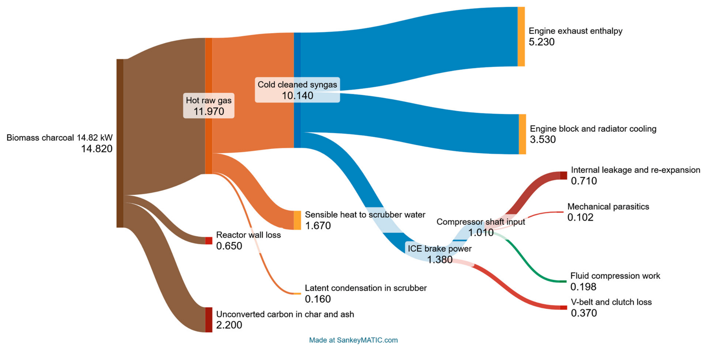
Because the cold gas efficiency of Table 4 is itself evaluated as CGE = ($\dot{\mathrm{V}}$_syngas·LHV_syngas)/(ṁ_fuel·LHV_fuel), the agreement between 7.63 × 4.79 = 10.15 kW and 0.684 × 14.82 = 10.14 kW is an algebraic identity to within the rounding of the CGE and is not an independent verification. It must be acknowledged that the gravimetric syngas route (8.87 kg/h × 4.12 MJ/kg = 36.5 MJ/h) and the carbon balance of Section 3.1 both derive the syngas throughput from the same orifice-based volumetric reading of 7.63 Nm³/h and are therefore not fully independent of it; what they verify is the internal consistency of the measured gas composition, apparent molecular weight and heating value, rather than the absolute flow magnitude. The adopted energy input of 10.14 kW is anchored instead on the gravimetrically measured charcoal rate and the measured cold gas efficiency, both of which are independent of the volumetric reading. Should the true area-averaged flow be lower than the center-line-derived value, the carbon accounted for in the gas would fall proportionally and the unconverted-carbon term of

Table 6. System-level energy balance for the DMD-Syngas configuration.

Node/Flow	Power (kW)	% of Biomass Input	Type	Loss Category/Remark
A. Primary input
Primary biomass input, (${\dot{Q}}_{biomass}$)	14.82	100	Input	1.84 kg/h × 29 MJ/kg
B. Gasification stage
B1. Reactor boundary (gasification)
(i) Reactor wall loss (radiation + convection)	0.65	4.4	Loss	Irrecoverable environmental loss
(ii) Unconverted carbon in char fines, ash and scrubber residue	2.20	14.8	Loss (closure)	Dominant reactor loss; corroborated by the carbon balance of 3.1
Reactor loss subtotal	2.85	19.2	Loss	(i) + (ii)
Hot raw gas leaving the reactor (chemical + sensible + latent)	11.97	80.8	Cascade	10.14 chemical + 1.67 sensible + 0.16 latent; ηhot-gas = 79.7% on a chemical-plus-sensible basis
B2. Gas-conditioning boundary (cyclone + wet scrubber + moisture separator)
(iii) Syngas sensible heat rejected to scrubber water (600 → 30 °C)	1.67	11.3	Loss	Rejected downstream of the reactor; recoverable in principle (Section 4.1)
(iv) Water-vapor condensation (latent)	0.16	1.1	Loss	Feedstock moisture (0.09 kg/h) + water–gas-shift water (0.14 kg/h)
Conditioning loss subtotal	1.83	12.3	Loss	(iii) + (iv)
Cold cleaned syngas delivered to ICE (CGE = 68.4%)	10.14	68.4	Cascade	Measured at the engine inlet, post-scrubber
C. Engine stage
Engine exhaust enthalpy	5.23	35.3	Loss	WHR potential
Engine block + radiator cooling loss	3.53	23.8	Loss	Partially recoverable
ICE brake power output	1.38	9.3	Cascade	Not a loss; carried forward to node D
D. Transmission stage
V-belt and clutch transmission loss	0.37	2.5	Loss	Friction/heat
Compressor shaft input	1.01	6.8	Cascade	Not a loss; carried forward to node E
E. Compressor stage
(E-i) Mechanical parasitics (lip seal, ring drag, slider pad)	~0.10	0.7	Loss (sub-item)	From ηmech,comp = 0.90 (assumed)
(E-ii) Internal leakage and clearance re-expansion	~0.71	4.8	Loss (sub-item)	Dominant; volumetric deficiency at 7.7–15.5% rated load
Compressor internal dissipation, (${\dot{W}}_{friction}$)	0.812	5.5	Loss	Dissipated within the compressor by internal leakage, re-expansion and parasitic friction (Section 2.1)
Fluid compression work, (${\dot{W}}_{comp,fluid}$)	0.198	1.34	Product of the biomass chain	Energy transferred to the R-134a refrigerant; (ηshaft→ref = 19.6%)
Closure check
Σ all loss rows (B + C + D + E)	14.622	98.66	—	4.68 + 8.76 + 0.37 + 0.812
Σ losses + fluid compression work	14.82	100	—	Balance closes identically

Note 1—Cascade versus loss rows. Rows marked Cascade (syngas chemical energy, ICE brake power, compressor shaft input) are intermediate energy carriers, not losses; each is the input to the following stage. Only rows marked Loss are additive, and their sum plus the fluid compression work equals the primary biomass input exactly (14.82 kW). Percentages are therefore all referenced to the same 14.82 kW denominator and must not be summed across the Cascade rows, which would double-count the downstream flows. Note 2—Ordering of the gasifier loss terms. The 4.68 kW conversion loss is dominated by unconverted carbon and char–ash carryover (2.20 kW, 47.0% of the conversion loss and 14.8% of the biomass input), followed by syngas sensible heat (1.67 kW, 35.7% of the loss, 11.3% of the input) and reactor wall losses (0.65 kW, 13.9% of the loss). Incomplete carbon conversion—not sensible-heat rejection—is thus the limiting mechanism of the present gasifier. Note 3—Closure term and its uncertainty. Item (iv) is obtained by closure and consequently inherits the accumulated uncertainty of the biomass rate (±2.7%), the syngas flow and composition (±3.1%) and the sensible-heat evaluation (±5.6%), giving u_c(iv) = ±0.14 kW. Items (i)–(iii) were determined independently from surface-temperature mapping, mole-fraction-weighted gas enthalpy and feedstock-moisture measurement, respectively. Note 4—Refrigeration output is not a fraction of the biomass input. The evaporator cooling capacity of 0.542 kW exceeds the 0.198 kW of fluid compression work because the majority of that thermal load is heat pumped from the cold space rather than energy supplied by the biomass chain (COPR = 0.542/0.198 = 2.74). It is therefore reported separately in Table 4 and not expressed as a percentage of the biomass input; the corresponding shaft-referred coefficient of performance is COPshaft = 0.542/1.01 = 0.537, and the biomass-referenced First-Law system efficiency is ηsys = 0.542/14.82 = 3.66%. Note 5—Reference for the reported 5.34%. The 5.34% figure quoted elsewhere in this work is referenced to the syngas chemical energy delivered to the engine (0.542/10.14), i.e., to a boundary drawn at the gasifier outlet, whereas the biomass-referenced value is 3.66%. Both are stated explicitly to avoid ambiguity in the system-boundary definition. Note 6—Partition of the compressor dissipation. Items E-i and E-ii are sub-items of the 0.812 kW lumped dissipation and are listed for interpretation only; they are not additive with the parent row in the closure check. Their partition rests on the assumed η_mech,comp = 0.90 (Section 2.6) and would require indicator-diagram or calorimetric shell measurement for confirmation (Section 4.4). Note 7—Two gasification sub-boundaries. The 4.68 kW aggregate previously reported as a single gasifier conversion loss is resolved here into a reactor-boundary loss of 2.85 kW (wall radiation and unconverted carbon) and a conditioning-train loss of 1.83 kW (sensible heat and latent condensation rejected to the scrubber water). Cold gas efficiency is defined at the outer boundary, i.e., at the engine inlet after the cyclone, wet scrubber and moisture separator, and is therefore 68.4%; the corresponding reactor-boundary hot-gas efficiency, which credits the sensible enthalpy of the raw gas, is 79.7%. The two sub-boundary losses sum identically to the 4.68 kW previously tabulated, so every downstream figure in Table 6 and Table 7 and every efficiency reported in this work is unchanged.

would rise correspondingly; a pitot traverse or a calibrated thermal-mass flow meter is therefore recommended to bound this term directly. The primary biomass thermal input of 14.82 kW corresponds to the measured DMD charcoal consumption rate of 1.84 kg/h and the gravimetric lower heating value of longan charcoal (29.0 MJ/kg, Table 4) and constitutes the single denominator against which all system-level First-Law and exergy efficiencies in this study are referenced. The 4.68 kW (31.6% of the biomass input) that separates the primary biomass energy from the cold cleaned syngas is generated across two physically distinct sub-boundaries rather than within the reactor alone and is resolved accordingly in Table 6.

Within the reactor boundary, 0.65 kW is lost as wall radiation and convection and 2.20 kW leaves as unconverted carbon in char fines, ash and scrubber residue, giving a reactor loss of 2.85 kW (19.2%) and a hot raw gas stream of 11.97 kW (80.8%) that carries 10.14 kW of chemical energy together with 1.67 kW of sensible heat and 0.16 kW of latent enthalpy. Within the gas-conditioning boundary, comprising the cyclone, the packed-bed wet scrubber and the moisture separator, the sensible and latent terms (1.83 kW, 12.3%) are transferred to the scrubber water, so that the gas reaching the engine inlet retains only its chemical energy of 10.14 kW. Cold gas efficiency is therefore a property of the combined reactor-plus-conditioning boundary (CGE = 10.14/14.82 = 68.4%), whereas the reactor alone converts 79.7% of the biomass energy into chemical plus sensible enthalpy. The wall loss is irrecoverable and can be addressed only by insulation, the unconverted-carbon term requires grate and residence-time modification, and the sensible-heat term is recoverable in principle by a recuperative intake or scrubber heat-recovery loop (Section 4.1) since it is rejected to a liquid stream rather than dissipated directly to the atmosphere. Sensible heat content of the producer gas stream above the ambient dead-state temperature (T₀ = 30 °C) is calculated as

$$Q_{sensible}={\dot{m}}_{syngas}\times c_{p,syngas}\times \left(T_{syngas}-T_0\right)$$

(12)

This conversion loss was resolved into the four terms tabulated in Table 6. Consistent with the boundary definition adopted above, two separate energy reference bases are maintained throughout this study: biomass chemical energy for gasification performance evaluation and syngas chemical energy for engine conversion analysis. The transition between these boundaries is quantified explicitly by the CGE and therefore does not constitute an inconsistency in the energy accounting. The syngas sensible heat was evaluated on a normal-volume basis as ${\dot{Q}}_{sensible}={\dot{m}}_{syngas}{\overline{C}}_p\left(T_{reactor,out}-T_{scrubber,out}\right)$, where ${\dot{m}}_{syngas}$ = 7.63 Nm³/h × 1.163 kg/Nm³ = 8.87 kg/h and ${\overline{C}}_p$ = 1.19 kJ/(kg·K) was obtained as the mole-fraction-weighted mean specific heat of the measured gas composition over 303–873 K. With the thermocouple-measured reactor outlet temperature of 600 °C and a scrubber outlet temperature of 30 °C, this yields ${\dot{Q}}_{sensible}$ = 1.67 ± 0.09 kW, equivalent to 11.3% of the biomass energy input and 35.7% of the conversion loss. The latent term of 0.16 kW corresponds to a total condensate rate of 0.24 kg/h, comprising the 0.09 kg/h of feedstock moisture entering with the charcoal and 0.14 kg/h of reaction water formed by the water–gas shift within the reduction zone; both streams are condensed in the wet scrubber upstream of the engine and are therefore excluded from the syngas chemical energy by definition of CGE. The reactor wall loss, obtained from surface-temperature mapping with combined convective and radiative coefficients, was 0.65 kW (4.4%). The remaining 2.20 kW (14.8% of the biomass input, 47.0% of the conversion loss) is attributed by closure to unconverted carbon leaving as char fines and ash, together with residual soot retained in the scrubber water. As an independent consistency check, the entire sensible-plus-latent duty rejected upstream of the engine is absorbed by the scrubber water.

For the combined sensible-plus-latent duty of 1.67 + 0.16 = 1.83 kW and the measured circulation rate of 2 L/min, the predicted water temperature rise is ΔTw = $\dot{Q}$(ṁ_w·c_p,w) = 1.83/(0.0333 × 4.18) = 13.1 K, a magnitude readily resolvable by the installed K-type thermocouples and therefore usable as a direct verification of the sensible-heat term. Direct calorimetric confirmation of the scrubber duty was not performed and is recommended for future work to validate the closure-derived unconverted-carbon term. The gasifier conversion loss is therefore governed primarily by incomplete carbon conversion rather than by sensible-heat rejection. The sensible heat associated with the syngas stream (1.67 kW) is explicitly excluded from the ICE energy input basis. While this heat is technically part of the total thermal output from the gasifier, it is diverted from the power conversion boundary to define the net energetic potential specifically available for mechanical work. This approach avoids inflating the conversion efficiency and ensures that the system boundary is strictly defined by the chemical energy content accessible for combustion within the engine, thereby maintaining a clear distinction between internal thermal management and thermodynamic conversion losses. Consequently, the ICE energy input basis is constrained to the chemical energy content of the syngas, providing a consistent thermodynamic reference for evaluating the engine performance independent of the gasifier’s thermal state. This yields 1.38 kW of brake power, corresponding to a 13.6% brake thermal efficiency based on the 10.14 kW chemical energy input from the syngas. In the absence of direct exhaust calorimetry, this total was apportioned using the manufacturer’s published heat-balance ratios (exhaust: 59.8%; cooling: 40.2%), yielding 5.23 kW and 3.53 kW, respectively—a partition broadly consistent with lumped-parameter models of small-scale ICE cooling systems reported in the literature [41]. The 0.28 kW difference between this derived total and an independent estimate based on exhaust-gas temperature alone is within the propagated measurement uncertainty (±0.31 kW, k = 2) and is fully attributed to instrumentation resolution limits rather than a systematic energy loss. Direct exhaust calorimetry is recommended in future work to independently validate this apportionment. From the 1.38 kW brake output, V-belt friction dissipates 0.37 kW. The residual 1.01 kW compressor shaft input is transmitted to the compressor, where an explicit refrigerant mass flow rate (ṁ_ref) of 0.003566 kg/s (12.84 kg/h)—derived from the evaporator cooling capacity (${\dot{Q}}_{cooling}$ = 0.542 kW) and specific enthalpy change (h₁ − h₄ = 152 kJ/kg), consistent with the value tabulated in Table 5—requires a fluid-side compression work (Ẇ_comp,fluid = ṁ_ref(h₂ − h₁)) of 0.198 kW. The calculated refrigerant flow rate was therefore considered thermodynamically consistent before being applied in the compressor work and condenser heat balance calculations. The remaining 0.812 kW of the shaft input is dissipated within the compressor as internal suction-valve leakage, clearance re-expansion and parasitic friction, and is rejected to the ambient partly through the casing and partly via the recirculated refrigerant, without contributing to the discharge enthalpy of the delivered stream (Section 2.1); this establishes a shaft-to-refrigerant conversion ratio (η_shaft→ref = Ẇ_comp,fluid/Ẇ_shaft = 19.6%), which represents the fraction of compressor shaft power transferred into refrigerant compression work rather than the conventional mechanical efficiency of the compressor mechanism. Therefore, the shaft-referred isentropic efficiency is not equivalent to the refrigerant-side isentropic efficiency. The former represents the overall conversion effectiveness from shaft power to useful refrigerant compression, whereas the latter evaluates only the thermodynamic irreversibility occurring during refrigerant compression. It should be emphasized that η_shaft→ref as defined here is not the conventional indicated-to-brake mechanical efficiency of a compressor (typically 85–95%) but rather the fraction of delivered shaft power that is converted into refrigerant compression work under the present operating point. The two quantities are not alternative estimates of the same property and must not be compared directly. Adopting a conventional mechanical efficiency of 90% for the compressor mechanism, the purely frictional component of the 0.812 kW residual amounts to approximately 0.10 kW, and the indicated work delivered to the gas is approximately 0.91 kW; since only 0.198 kW appears as a net enthalpy rise in the delivered stream, the remaining ≈0.71 kW represents repeated compression and re-expansion of refrigerant that leaks back to the suction plenum. It should be noted that clearance re-expansion by itself is a nearly reversible process that lowers the volumetric efficiency without consuming indicated work; the dissipative fraction of this residual therefore arises specifically from suction- and discharge-valve leakage, blow-by past the piston rings, and throttling across the reed valves, whereas clearance volume acts to amplify the leakage path by reducing the delivered mass per revolution. This attribution is quantitatively self-consistent: referring to the swept mass flow of 68 kg/h (0.01889 kg/s, Section 2.1), the indicated work corresponds to 0.909/0.01889 ≈ 48 kJ/kg, i.e., 87% of the measured fluid-side enthalpy rise of 55.5 kJ/kg. The compressor is therefore performing very nearly the full compression duty on the swept mass, of which only ≈19% is actually delivered to the condenser—a signature of internal recirculation, not of mechanical drag, since a purely frictional 0.71 kW deficit would leave the indicated work far below the swept-mass compression requirement. It must nevertheless be stated explicitly that a steady-state control-volume balance drawn around the compressor admits only two exit paths for the shaft input, namely the enthalpy rise of the delivered stream and the shell heat loss, so that the 0.812 kW residual and the 0.05–0.23 kW shell conductance estimated in Section 2.1 cannot be reconciled simultaneously with the enthalpy-derived mass flow rate. The internal-recirculation mechanism identified above explains the work balance but does not by itself close the energy balance; the residual discrepancy of approximately 0.6 kW is therefore reported as an open item that requires either calorimetric shell measurement or direct Coriolis metering of the refrigerant flow for definitive resolution (Section 4.4), and it constitutes the principal reason why η_shaft→ref is reported as a conservative bound rather than as a settled component characteristic. The low value of η_shaft→ref is therefore predominantly a volumetric rather than a mechanical deficiency, consistent with the apparent volumetric efficiency of ≈19% established in Section 2.1, and it does not imply a mechanical efficiency outside the conventional 85–95% range. The atypically low value of η_shaft→ref (19.6%) is a direct consequence of operating an automotive swash-plate compressor at only 7.7–15.5% of its rated cooling capacity, at which the fixed clearance volume and the tension-independent leakage paths of the suction reed valves constitute a disproportionately large fraction of the swept duty; the residual mechanical parasitics (shaft lip-seal friction, piston-ring drag and slider-pad shearing) account for only ≈0.10 kW of the 0.812 kW residual. The low conversion ratio therefore reflects severe volumetric under-utilization at fractional load and does not indicate a mechanically defective unit.

$$Q_{cond}=Q_{cooling}+W_{comp,fluid}=0.542+0.198=0.740 \mathrm{k}\mathrm{W}$$

(13)

With W_comp,fluid harmonized at 0.198 kW, the condenser heat rejection (Q_cond) is robustly closed at 0.740 kW, ensuring that the input parameters for the condenser exergy destruction (Ex_dest,cond) and overall system exergy efficiency in Table 7 remain thermodynamically consistent.

Table 7. Component-level exergy analysis of the DMD-Syngas system.

Component	DMD	DMD	DMD	DMD	Share of Exdest,sys (%)	EPG	EPG	EPG	EPG	Share of Exdest,sys (%)
	Exin (kW)	Exout (kW)	Exdest (kW)	ε (%)		Exin (kW)	Exout (kW)	Exdest (kW)	ε (%)
Downdraft gasifier + syngas conditioning train	15.56	10.54	5.02	67.7	32.4	18.07	12.24	5.83	67.7	32.4
ICE	10.54	1.38	9.16	13.1	59.13	12.24	1.6	10.64	13.1	59.1
Belt–clutch transmission	1.38	1.01	0.37	73.2	2.39	—	—	—	—
AC alternator	—	—	—	—		1.6	1.28	0.32	80.0	1.8
Electric induction motor	—	—	—	—		1.28	1.02	0.26	79.7	1.4
Compressor internal dissipation	0.812	0	0.812	0	5.24	0.821	0	0.821	0	4.6
Compressor, refrigerant side	0.198	0.114	0.084	57.6	0.54	0.199	0.114	0.085	57.3	0.47
Condenser	0.114	0.110	0.004	96.5 *	0.03	0.114	0.11	0.004	96.5 *	0.02
Expansion valve	0.110	0.082	0.028	N/A **	0.18	0.11	0.082	0.028	N/A **	0.16
Evaporator	0.082	0.0685	0.0135	83.5	0.09	0.082	0.0685	0.0135	83.5	0.08
SYSTEM TOTAL	15.56	0.0685	15.49	0.44	100	18.07	0.0685	18	0.38	100

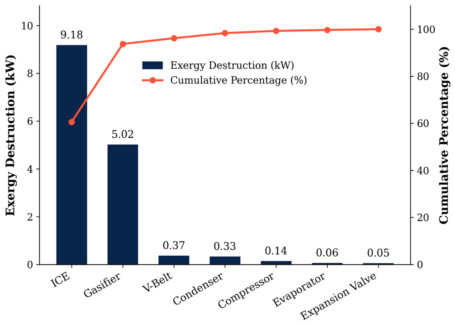
Note 1 * For the condenser, which rejects heat to the environment without recovery, no useful exergy product exists; the value reported is the refrigerant-stream exergy transit ratio Ex_out/Ex_in rather than a product-to-fuel exergetic efficiency. ** Throttling is a purely dissipative process for which the fuel–product exergetic efficiency is undefined; the entire incoming stream exergy decrement is destroyed, with ${\dot{Ex}}_{dest,valve}$ = ${\dot{m}}_{dest,valve}$T₀(s₄ − s₃) = (0.003566 × 303.15) × (1.1878 − 1.1621) = 0.028 kW. Note 2—Biomass reference. The primary exergy input is evaluated as Ex_biomass = φ m_fuel LHV with φ = 1.05 and LHV = 29 MJ/kg. DMD: 1.84 kg/h → 14.82 kW energy → 15.56 kW exergy. EPG: 2.1367 kg/h → 17.21 kW energy → 18.07 kW exergy. Both configurations are evaluated at the same measured CGE of 68.4% and the same syngas chemical-exergy factor (1.04), so that the 13.89% higher EPG fuel consumption propagates consistently through every downstream row. Note 3—Cascade closure. Each row takes as its input the output of the preceding row; consequently, ∑Ex_dest = Ex_in,sys−Ex_out,sys is satisfied identically (DMD: 15.56 − 0.0685 = 15.49 kW; EPG: 18.07 − 0.0685 = 18.00 kW). The EPG shaft power delivered to the compressor (1.02 kW) matches the value measured under DMD (1.01 kW) to within 1%, confirming that both drive trains supply the same mechanical duty to an identical refrigeration loop. Note 4—Separation of shaft-level dissipation. The measured compressor shaft power (1.01 kW for DMD; 1.02 kW for EPG) exceeds the fluid-side compression work obtained from the refrigerant enthalpy rise (W_comp,fluid = m_ref (h₂ − h₁) = 0.198 kW) by 0.812 kW. This residual is reported as a distinct mechanical-dissipation row (row 4/5) rather than being distributed among the heat exchangers because it is dissipated internally within the compressor by suction-valve leakage, clearance re-expansion and parasitic friction, and it is ultimately rejected at the dead-state temperature (Section 2.1); therefore, it performs no thermodynamic function within the refrigerant control volume. Its exergetic efficiency is zero by definition, and the shaft-to-refrigerant conversion ratio is ηshaft→ref = 0.198/1.01 = 19.6%. Note 5—Loop-referenced heat-exchanger rows. Because the closed refrigerant loop receives only W_comp,fluid = 0.198 kW and delivers Exproduct = Qcooling (T₀/T_L − 1) = 0.0685 kW, the total irreversibility generated inside the loop is bounded at 0.1295 kW. The compressor, condenser, expansion-valve and evaporator rows are therefore reported on this loop-referenced basis—i.e., as the exergy carried by the refrigerant stream relative to its own compression work input—and not as absolute stream exergies. The individual condenser, expansion-valve and evaporator destructions are each obtained directly from the entropy generation of the corresponding process, Ėx_dest = T₀·ṁ_ref·Δs_gen, without any proportional normalization. Their sum (0.004 + 0.028 + 0.0135 = 0.0455 kW), added to the compressor destruction of 0.084 kW, reproduces the loop bound of Ẇ_comp,fluid − Ėx_cool = 0.198 − 0.0685 = 0.1295 kW identically, so that Second-Law consistency is satisfied by construction rather than imposed by normalization. Note 6—Dominant irreversibilities. For both configurations, the internal-combustion engine is the largest single source of exergy destruction (59.13% for DMD, 59.2% for EPG), followed by the gasifier (32.4% in both cases). The two drive-train pathways differ only marginally in exergetic terms (2.4% for the DMD belt–clutch versus 3.2% for the EPG alternator–motor chain), confirming that the 13.89% fuel-consumption penalty of EPG originates from the double electromechanical conversion rather than from any difference in refrigeration performance. The refrigerant loop itself accounts for less than 0.9% of the total destruction; the small absolute magnitude of the system exergy efficiency (0.44% for DMD, 0.38% for EPG) is thus set almost entirely by the thermochemical and combustion stages upstream of the compressor and not by the refrigeration circuit. Note 7—Composition of the gasification-boundary irreversibility. The 5.02 kW attributed to the gasifier row is the exergy difference across the combined reactor-and-conditioning boundary and therefore comprises both true internal destruction and external exergy losses. The dominant external terms are the chemical exergy of the unconverted carbon leaving as char fines and ash (≈2.3 kW, obtained as 2.20 kW × φ = 1.05) and the thermal exergy of the raw gas rejected to the scrubber water, evaluated as $\dot{m}\overline{c}p$[(T − T₀) − T₀ln(T/T₀)] = 0.73 kW at the measured 873 K reactor outlet against a 303.15 K dead state. The residual, of order 1.6–2.0 kW, represents genuine destruction by the exothermic oxidation and endothermic reduction reactions. Because the external terms are recoverable in principle whereas the destroyed fraction is not, the gasification row discussed in Section 2.7 should be read as an aggregate improvement potential] rather than as pure irreversibility. The tabulated Ex_dest values are retained on the difference basis so that the cascade closure of Note 2 is preserved. N/A denotes "not applicable"—the PV-Battery configuration does not require biomass fuel, whereas both biomass-powered configurations (EPG and DMD) do not incorporate electrochemical battery storage.

Table 7. Component-level exergy analysis of the DMD-Syngas system.

Component	DMD	DMD	DMD	DMD	Share of Exdest,sys (%)	EPG	EPG	EPG	EPG	Share of Exdest,sys (%)
	Exin (kW)	Exout (kW)	Exdest (kW)	ε (%)		Exin (kW)	Exout (kW)	Exdest (kW)	ε (%)
Downdraft gasifier + syngas conditioning train	15.56	10.54	5.02	67.7	32.4	18.07	12.24	5.83	67.7	32.4
ICE	10.54	1.38	9.16	13.1	59.13	12.24	1.6	10.64	13.1	59.1
Belt–clutch transmission	1.38	1.01	0.37	73.2	2.39	—	—	—	—
AC alternator	—	—	—	—		1.6	1.28	0.32	80.0	1.8
Electric induction motor	—	—	—	—		1.28	1.02	0.26	79.7	1.4
Compressor internal dissipation	0.812	0	0.812	0	5.24	0.821	0	0.821	0	4.6
Compressor, refrigerant side	0.198	0.114	0.084	57.6	0.54	0.199	0.114	0.085	57.3	0.47
Condenser	0.114	0.110	0.004	96.5 *	0.03	0.114	0.11	0.004	96.5 *	0.02
Expansion valve	0.110	0.082	0.028	N/A **	0.18	0.11	0.082	0.028	N/A **	0.16
Evaporator	0.082	0.0685	0.0135	83.5	0.09	0.082	0.0685	0.0135	83.5	0.08
SYSTEM TOTAL	15.56	0.0685	15.49	0.44	100	18.07	0.0685	18	0.38	100

Note 1 * For the condenser, which rejects heat to the environment without recovery, no useful exergy product exists; the value reported is the refrigerant-stream exergy transit ratio Ex_out/Ex_in rather than a product-to-fuel exergetic efficiency. ** Throttling is a purely dissipative process for which the fuel–product exergetic efficiency is undefined; the entire incoming stream exergy decrement is destroyed, with ${\dot{Ex}}_{dest,valve}$ = ${\dot{m}}_{dest,valve}$T₀(s₄ − s₃) = (0.003566 × 303.15) × (1.1878 − 1.1621) = 0.028 kW. Note 2—Biomass reference. The primary exergy input is evaluated as Ex_biomass = φ m_fuel LHV with φ = 1.05 and LHV = 29 MJ/kg. DMD: 1.84 kg/h → 14.82 kW energy → 15.56 kW exergy. EPG: 2.1367 kg/h → 17.21 kW energy → 18.07 kW exergy. Both configurations are evaluated at the same measured CGE of 68.4% and the same syngas chemical-exergy factor (1.04), so that the 13.89% higher EPG fuel consumption propagates consistently through every downstream row. Note 3—Cascade closure. Each row takes as its input the output of the preceding row; consequently, ∑Ex_dest = Ex_in,sys−Ex_out,sys is satisfied identically (DMD: 15.56 − 0.0685 = 15.49 kW; EPG: 18.07 − 0.0685 = 18.00 kW). The EPG shaft power delivered to the compressor (1.02 kW) matches the value measured under DMD (1.01 kW) to within 1%, confirming that both drive trains supply the same mechanical duty to an identical refrigeration loop. Note 4—Separation of shaft-level dissipation. The measured compressor shaft power (1.01 kW for DMD; 1.02 kW for EPG) exceeds the fluid-side compression work obtained from the refrigerant enthalpy rise (W_comp,fluid = m_ref (h₂ − h₁) = 0.198 kW) by 0.812 kW. This residual is reported as a distinct mechanical-dissipation row (row 4/5) rather than being distributed among the heat exchangers because it is dissipated internally within the compressor by suction-valve leakage, clearance re-expansion and parasitic friction, and it is ultimately rejected at the dead-state temperature (Section 2.1); therefore, it performs no thermodynamic function within the refrigerant control volume. Its exergetic efficiency is zero by definition, and the shaft-to-refrigerant conversion ratio is ηshaft→ref = 0.198/1.01 = 19.6%. Note 5—Loop-referenced heat-exchanger rows. Because the closed refrigerant loop receives only W_comp,fluid = 0.198 kW and delivers Exproduct = Qcooling (T₀/T_L − 1) = 0.0685 kW, the total irreversibility generated inside the loop is bounded at 0.1295 kW. The compressor, condenser, expansion-valve and evaporator rows are therefore reported on this loop-referenced basis—i.e., as the exergy carried by the refrigerant stream relative to its own compression work input—and not as absolute stream exergies. The individual condenser, expansion-valve and evaporator destructions are each obtained directly from the entropy generation of the corresponding process, Ėx_dest = T₀·ṁ_ref·Δs_gen, without any proportional normalization. Their sum (0.004 + 0.028 + 0.0135 = 0.0455 kW), added to the compressor destruction of 0.084 kW, reproduces the loop bound of Ẇ_comp,fluid − Ėx_cool = 0.198 − 0.0685 = 0.1295 kW identically, so that Second-Law consistency is satisfied by construction rather than imposed by normalization. Note 6—Dominant irreversibilities. For both configurations, the internal-combustion engine is the largest single source of exergy destruction (59.13% for DMD, 59.2% for EPG), followed by the gasifier (32.4% in both cases). The two drive-train pathways differ only marginally in exergetic terms (2.4% for the DMD belt–clutch versus 3.2% for the EPG alternator–motor chain), confirming that the 13.89% fuel-consumption penalty of EPG originates from the double electromechanical conversion rather than from any difference in refrigeration performance. The refrigerant loop itself accounts for less than 0.9% of the total destruction; the small absolute magnitude of the system exergy efficiency (0.44% for DMD, 0.38% for EPG) is thus set almost entirely by the thermochemical and combustion stages upstream of the compressor and not by the refrigeration circuit. Note 7—Composition of the gasification-boundary irreversibility. The 5.02 kW attributed to the gasifier row is the exergy difference across the combined reactor-and-conditioning boundary and therefore comprises both true internal destruction and external exergy losses. The dominant external terms are the chemical exergy of the unconverted carbon leaving as char fines and ash (≈2.3 kW, obtained as 2.20 kW × φ = 1.05) and the thermal exergy of the raw gas rejected to the scrubber water, evaluated as $\dot{m}\overline{c}p$[(T − T₀) − T₀ln(T/T₀)] = 0.73 kW at the measured 873 K reactor outlet against a 303.15 K dead state. The residual, of order 1.6–2.0 kW, represents genuine destruction by the exothermic oxidation and endothermic reduction reactions. Because the external terms are recoverable in principle whereas the destroyed fraction is not, the gasification row discussed in Section 2.7 should be read as an aggregate improvement potential] rather than as pure irreversibility. The tabulated Ex_dest values are retained on the difference basis so that the cascade closure of Note 2 is preserved. N/A denotes "not applicable"—the PV-Battery configuration does not require biomass fuel, whereas both biomass-powered configurations (EPG and DMD) do not incorporate electrochemical battery storage.

From the 1.01 kW total shaft power supplied to the compressor, 0.198 kW is effectively converted into fluid compression work (W_comp,fluid), while the remaining 0.812 kW is dissipated internally by suction-valve leakage, clearance re-expansion and parasitic friction and rejected to the ambient partly through the casing and partly via the recirculated refrigerant (Section 2.1), establishing a consistent shaft-to-refrigerant conversion ratio (η_shaft→ref = 19.6%) that closes the system energy balance. To avoid conflation, these processes must be evaluated via two distinct control volumes: the shaft mechanical balance (W_shaft = W_comp,fluid + ${\dot{W}}_{\mathrm{d}\mathrm{i}\mathrm{s}\mathrm{s},\mathrm{c}\mathrm{o}\mathrm{m}\mathrm{p}}$ = 0.198 + 0.812 = 1.01 kW) and the refrigerant-circuit thermal balance (Q_cond = Q_evap + W_comp,fluid = 0.542 + 0.198 = 0.740 kW). Notably, the 0.812 kW shaft-level dissipation is confined to the mechanical shaft level, while Q_evap is governed by refrigerant thermodynamics and does not appear in the shaft-level equation. To rigorously account for the primary biomass resource utilization, the overall First Law system efficiency must be defined based on the initial biomass chemical energy input

$$Q_{biomass}={\displaystyle \frac{Q_{input}}{CGE}}={\displaystyle \frac{10.14}{0.684}}=14.84 \mathrm{k}\mathrm{W}$$

(14)

The overall First Law system efficiency, evaluated from the primary biomass energy input (14.82 kW) to the useful cooling output (0.542 kW), is

$${\eta }_{system}={\displaystyle \frac{{\dot{Q}}_{cooling}}{{\dot{Q}}_{biomass}}}={\displaystyle \frac{0.542}{14.82}}=3.66\%$$

(15)

where ${\dot{Q}}_{\mathrm{c}\mathrm{o}\mathrm{o}\mathrm{l}\mathrm{i}\mathrm{n}\mathrm{g}}$ originates from the refrigerant-side evaporator load, not from the mechanical shaft. For reference, the syngas-to-cooling efficiency, which excludes the gasifier conversion stage, is defined as η_syngas = Q_cooling/$\dot{\mathrm{Q}}$_input = 0.542/10.14 = 5.34%. To recover the primary-energy boundary, this syngas-to-cooling value (5.34%) is multiplied by the gasifier cold gas efficiency (CGE = 68.4%), returning the same biomass-to-cooling system efficiency of 3.66% (3.65% before rounding of the intermediate values) obtained directly in Equation (14). As summarized in Table 6, the primary biomass thermal input of 14.82 kW is progressively dissipated across the conversion chain: the conversion to syngas entails gasifier conversion loss of 4.68 kW (31.6% of biomass input), followed by engine exhaust enthalpy at 5.23 kW (35.3%) and engine block cooling loss at 3.53 kW (23.8%).

Thermodynamically, the primary drivers of energy degradation in the integrated system are high-temperature thermal dissipation and chemical irreversibilities. The gasifier losses (31.6%) are predominantly due to the endothermic nature of reduction reactions and convective/radiative jacket losses, while the engine losses (exhaust at 35.3% and cooling at 23.8%) represent unavoidable thermal rejection constraints dictated by the second law of thermodynamics for small-scale internal combustion cycles [41].

The V-belt transmission contributes a further 0.37 kW (2.5%) of frictional loss. The remaining 1.01 kW is delivered to the compressor shaft, from which 0.812 kW (5.5%) is dissipated within the compressor by internal suction-valve leakage, clearance re-expansion and parasitic friction (Section 2.1), leaving 0.198 kW (1.34%) as the actual fluid compression work (W_comp,fluid) added to the refrigerant. It is important to note that the useful cooling output (Q_cooling) of 0.542 kW is thermal energy extracted from the cold space, not a direct residual of the biomass energy, ultimately yielding an overall system efficiency (η_system) of 3.66%. The energy flow cascade through each subsystem for both DMD and EPG configurations is depicted in Figure 5.

However, it should be noted that this 31.6% gasifier conversion loss is dominated by unconverted carbon leaving as char fines, ash and scrubber residue (2.20 kW, 47.0% of the loss), with the syngas sensible-heat fraction contributing 1.67 kW (35.7% of the loss, 11.3% of the biomass input). Only the sensible-heat term is recoverable in principle through a scrubber or intake heat-recovery loop; the unconverted-carbon term instead requires improvements in grate design, reduction-zone residence time and char-fines retention. To maintain consistent thermodynamic interpretation throughout this study, all energy streams are rigorously classified into three distinct categories: ‘Useful Energy Output’ for work conversion, ‘Thermal Recovery Potential’ for streams possessing high-grade exergy suitable for waste heat recovery, and ‘Environmental Dissipation’ for energy rejected into the surroundings. This systematic taxonomy ensures that all energy balance narrations, including the Sankey diagram (Figure 5) and performance summary (Table 6), remain methodologically aligned and strictly distinct from one another.

Figure 5 presents a quantitative Sankey diagram of the system energy cascade for the DMD-Syngas configuration, with stream widths proportional to power magnitude (kW). The EPG pathway is superimposed with dashed boundaries to highlight the two additional conversion stages (alternator and electric motor) that contribute the incremental 13.89% fuel penalty. To ensure a transparent interpretation of the loss distribution, the system boundary must distinguish between irreversible heat losses to the environment and the usable thermal energy content of the syngas.

Specifically, Figure 5 shows that carbon conversion, not thermal rejection, is the limiting mechanism of the present gasifier: the unconverted-carbon stream (14.8% of the biomass input) exceeds the syngas sensible-heat stream (11.3%) by a factor of 1.34; the former arises inside the reactor boundary and the latter inside the conditioning boundary, so the two are addressed by different design measures and should not be pooled into a single gasifier loss. The sensible heat is nonetheless rejected in the wet scrubber upstream of the engine and is excluded from the cold-gas chemical energy by definition of CGE; assuming a recuperator effectiveness of 50–70%, 0.84–1.17 kW could be returned as preheated gasification air, corresponding to a potential charcoal saving of 5.7–7.9%. This is a meaningful but secondary improvement relative to the unconverted-carbon loss, and the two measures should be pursued in that order of priority. Because this sensible heat is removed before combustion rather than dissipated directly to the environment as reactor-wall loss, future designs could integrate an engine-intake or scrubber heat-recovery loop to raise the effective cold gas efficiency.

2.7. Component-Level Exergy Analysis

An exergy analysis based on the Second Law of Thermodynamics was performed to identify the magnitudes and locations of thermodynamic irreversibility within the system. For each component, the exergy efficiency ε is defined uniformly as the ratio of productive exergy output to exergy input (ε = Ėx_out/Ėx_in), where “productive output” denotes the exergy stream that serves a useful thermodynamic purpose in the downstream subsystem. Exergy destruction within each component is calculated from the component exergy balance as Ėx_dest = Ėx_in − Ėx_out, consistent with Szargut’s reference-environment model at T₀ = 303.15 K and P₀ = 101.325 kPa. For the compressor component, the exergy destruction was evaluated only within the refrigerant control volume using the refrigerant-side enthalpy changes. The shaft-level dissipation (Ẇ_diss,comp = 0.812 kW), which is degraded internally within the compressor and ultimately rejected at the dead-state temperature (Section 2.1), was treated separately as mechanical dissipation and excluded from the refrigerant-cycle exergy destruction. The exergy of the cooling effect is referenced to the mean product temperature of the ice load (269.15 K) rather than to the refrigerant evaporating temperature (263.15 K), so that the finite-temperature-difference irreversibility of the evaporator is retained within the component boundary. All exergy flow rates are expressed in kilowatts (kW), and ε_values are reported as percentages (%). The exergy content of the syngas stream was approximated as its chemical exergy, calculated from the composition and LHV:

$${Ex}_{syngas}= \phi LHV {\dot{m}}_{syngas}$$

(16)

In Table 7, the exergy efficiency ε (%) is defined uniformly as ε = Ex_out/Ex_in × 100% for all components, where Ex_out represents the exergetic product, and Ex_in represents the exergetic fuel for each component boundary. The exergy destruction rate Ex_dest (kW) is derived as Ex_dest = Ex_in − Ex_out at steady state, consistent with the Gouy–Stodola theorem. These two quantities occupy separate columns and should not be compared directly. φ represents the chemical exergy-to-LHV ratio for the syngas mixture (1.04), yielding a syngas chemical exergy of 10.54 kW—which constitutes the gasifier exergy output, not the system exergy input. Component-level exergy balances were evaluated at the measured dead-state ambient temperature (T0 = 303.15 K). The useful exergy product of the refrigeration system is the exergy transferred from the cold space at the evaporator temperature, defined as Ex_product = Q_cooling × (T₀/T_L − 1) = 0.542 × [(303.15/263.15) − 1] = 0.0824 kW. This product exergy—not the cooling capacity itself—is the correct exergetic output of a refrigeration system, since the 0.542 kW thermal load is delivered at 263.15 K and therefore carries only 12.6% of its energy magnitude as work potential relative to the 303.15 K dead state; referenced instead to the 263.15 K evaporating temperature, the factor would be 15.2%, giving 0.0824 kW. The system-level exergy balance closes as follows: total exergy input Ėx_in,sys = 15.56 kW (chemical exergy of the raw biomass feedstock); total exergy output Ėx_out,sys = 0.0685 kW (refrigeration product exergy referenced to the mean ice-product temperature of 269.15 K); and total system exergy destruction Ėx_dest,sys = 15.56 − 0.0685 = 15.49 kW, yielding a biomass-referenced system exergy efficiency of ε_sys = 0.0685/15.56 = 0.44%. Referencing the product exergy instead to the refrigerant evaporating temperature of 263.15 K would give 0.0824 kW and ε_sys = 0.53%; that value is reported here only as the upper bound of the admissible range since it excludes the finite-temperature-difference irreversibility between the evaporating refrigerant and the ice load and would therefore render the evaporator reversible.

The IC engine accounts for 9.16/15.49 = 59.1% of total exergy destruction, followed by the gasifier at 5.02/15.49 = 32.4%. In the open-drive reciprocating compressor, the exergy balance is evaluated on the refrigerant-side control volume: the exergetic fuel is the shaft work actually delivered to the fluid (Ex_in = W_comp,fluid = 0.198 kW), and the exergetic product is the flow-exergy rise of the refrigerant across the compressor (Ex_out = ṁ[(h₂ − h₁) − T₀(s₂ − s₁)] = 0.113 kW). This yields a compressor exergy destruction of Ex_dest,comp = 0.198 − 0.113 = 0.085 kW and an exergetic efficiency of ε_comp = 0.113/0.198 = 57.1%, in agreement with the Gouy–Stodola result of Ex_dest = T₀·ṁ·(s₂ − s₁) = 0.085 kW. For internal consistency, the refrigeration loop must close on its own exergy input: with Ėx_in,cycle = Ẇ_comp,fluid = 0.198 kW and Ėx_product = 0.0685 kW, the total destruction inside the closed refrigerant loop is bounded at 0.1295 kW, of which the compressor accounts for 0.084 kW and the condenser, expansion valve and evaporator together for 0.0455 kW. The condenser, valve and evaporator rows of Table 7 are therefore reported on this loop-referenced basis rather than as absolute stream exergies, and the 0.812 kW of shaft-level dissipation is listed as a separate mechanical-dissipation row, so that the component destructions sum exactly to Ėx_dest,sys = 5.02 + 9.16 + 0.37 + 0.812 + 0.1295 = 15.49 kW. Consistently, the expansion-valve exergy destruction is evaluated directly from the entropy generation of the isenthalpic process, ${\dot{Ex}}_{dest,vale}$ = ${\dot{m}}_{dest,valve}$T₀(s₄ − s₃), and the evaporator destruction from ${\dot{Ex}}_{dest,evap}$ = $\dot{m}$_ref (Ex4 − Ex1) − ${\dot{Ex}}_{cool}$, so that the component-wise sum reproduces the overall refrigerant-side destruction obtained independently from T₀ [(${\dot{Q}}_{cond}$/T₀) − (${\dot{Q}}_{evap}$/T_L)] = 0.1295 kW.

All exergy values are referenced to a dead state of T₀ = 303.15 K and P₀ = 101.325 kPa. The exergy of the cooling effect is referenced to the mean product temperature of the ice load (−4 °C) rather than to the refrigerant evaporating temperature (−10 °C), so that the finite-temperature-difference irreversibility of the evaporator is retained within the component boundary; referencing instead to the evaporating temperature would give ${\dot{Ex}}_{cool}$= 0.0824 kW and would render the evaporator exergy destruction identically zero, which is physically inadmissible. The tabulated ${\dot{Ex}}_{dest}$ of the gasifier, ICE and compressor internal-dissipation rows aggregates internal exergy destruction with exergy losses discharged to the environment (flue gas, coolant and casing heat rejection) since neither stream is recovered in the present configuration; for the compressor, the casing rejection at approximately 348 K carries 0.105 kW of the 0.812 kW as recoverable exergy loss rather than destruction. To remain consistent with the refrigerant-side control volume used throughout this analysis, the exergy input to the compressor is taken as the work actually delivered to the fluid (W_comp,fluid = 0.198 kW) rather than the total shaft power (W_shaft = 1.01 kW). The 0.812 kW of shaft-level dissipation, being dissipated internally and ultimately degraded to the dead-state temperature T₀, carries negligible exergy into the refrigerant stream delivered to the condenser and is accounted for separately in the shaft mechanical balance of Section 2.6. The resulting exergetic efficiency (ε_comp = 57.1%) is marginally higher than the isentropic efficiency (η_is = 52.3%), as expected for an adiabatic compressor whose reversible-work reference differs slightly from the isentropic-work reference. The two metrics are therefore mutually consistent, both reflecting the fluid-side compression irreversibility within a single, well-defined control volume. The Reciprocating Compressor row is evaluated on the refrigerant-side work basis, where the exergetic fuel is the shaft work delivered to the fluid (Ex_in = W_comp,fluid = 0.198 kW), and the exergetic product is the flow-exergy rise of the refrigerant across the compressor (Ex_out = ṁ[(h₂ – h₁) − T₀(s₂ – s₁)] = 0.113 kW). This row therefore quantifies the intrinsic compression irreversibility and is not part of the absolute exergy-stream cascade feeding the condenser; the 0.812 kW of shaft-level dissipation is dissipated internally within the compressor (Section 2.1) and is accounted for separately in the shaft mechanical balance of Section 2.6.

The true system exergy input is the chemical exergy of the raw biomass feedstock, Ex_biomass = φ_biomass · $\dot{\mathrm{Q}}$_biomass = 1.05 × 14.82 = 15.56 kW, where φ_biomass = 1.05 is the chemical-exergy-to-LHV ratio for high-fixed-carbon longan charcoal estimated from the Szargut reference-environment correlation. The syngas chemical exergy (Ex_syngas = φ_syngas · LHV · $\dot{\mathrm{V}}$_syngas = 1.04 × 10.14 = 10.54 kW) therefore constitutes the gasifier exergy output delivered to the engine boundary, not the system exergy input. Referencing the useful cold-product exergy to this primary biomass exergy input yields the system exergy efficiency ε_sys = Ex_product/Ex_biomass = 0.0685/15.56 = 0.44%, on a biomass-referenced basis consistent with the First-Law system efficiency (3.66%). The system exergy output (Ex_out = 0.0685 kW) is the refrigeration product exergy = Q_cooling × (T₀/T_L − 1), representing the useful thermodynamic work potential of the cold effect delivered at T_L = 269.15 K.

The biomass-referenced exergy efficiency (0.44%) and the biomass-referenced First-Law efficiency (3.66%) are not two estimates of the same performance attribute, and their ratio must not be read as a performance gap. That ratio is fixed by definition at (T₀/T_ice − 1)/φ_biomass = 0.126/1.05 = 0.120—the Carnot exergy factor of the cold product divided by the chemical-exergy-to-LHV ratio of the feedstock—and is therefore independent of how well the machine is built; 3.66% × 0.120 returns 0.44% identically. The Second-Law metric is reported alongside the First-Law metric because it additionally accounts for the work potential degraded in delivering the refrigeration effect at 263.15 K against a 303.15 K dead state, which First-Law accounting cannot express. In the EPG configuration, V-belt transmission is replaced by the AC alternator–electric motor cascade; accordingly, the V-belt row is not applicable (N/A) for EPG, and the alternator/motor rows are not applicable for DMD. Both configurations deliver the same refrigeration product exergy (Ėx_out = 0.0685 kW), but EPG requires a larger primary biomass exergy input owing to its 13.89% higher fuel consumption. For the EPG configuration, the measured fuel rate of 2136.7 g/h corresponds to a primary biomass input of 17.21 kW (Ėx_biomass = 1.05 × 17.21 = 18.07 kW) and, at the same measured CGE of 68.4%, to a syngas chemical energy of 11.77 kW (Ėx_syngas = 12.24 kW). The engine therefore delivers 1.60 kW of brake power, of which the alternator (ε_alternator = 80.0%) and the induction motor (ε_motor = 79.7%) transmit 1.02 kW to the compressor shaft—matching the 1.01 kW measured under DMD and thereby closing the EPG cascade. The induction motor employed in the EPG train is rated at 1.1 kW continuous duty, so that the 1.02 kW shaft output corresponds to 93% of its nameplate rating; the measured conversion efficiency of 79.7% is consistent with IE1-class performance for fractional-kilowatt motors operating near rated load under variable-frequency supply. The resulting EPG exergy destruction is 18.00 kW, and its biomass-referenced exergy efficiency is ε_sys = 0.0685/18.07 = 0.38%, compared with 0.44% for DMD.

An exergy assessment based on Szargut’s model revealed that the internal combustion engine was the single dominant contributor to thermodynamic irreversibility (9.16 kW, 59.2% of total exergy destruction, ε = 13.1%), followed by the gasifier (5.02 kW, 32.4%, ε = 67.7%); together they account for 91.6% of total system exergy destruction. To mitigate these losses, two optimization pathways were therefore evaluated. Reducing the 0.65 kW reactor wall loss of Table 6 by 15% through improved insulation recovers 0.10 kW, and recycling 30–35% of the 5.23 kW exhaust enthalpy (1.57–1.83 kW) to preheat the gasification air recovers approximately 1.05 kW as exergy at the measured exhaust temperature. Combined, these modifications reduce total system exergy destruction by 1.15 kW, i.e., approximately 7.4%, from 15.49 kW to 14.34 kW. The distribution of component-level exergy destruction is visually illustrated in the Pareto chart in Figure 6.

2.8. Life-Cycle Cost (LCC) Methodology Framework

The techno-economic baseline of the system was quantified using an LCC model evaluated over a 10-year analysis horizon (n = 10) with a discount rate of r = 6% per annum, consistent with the Bank of Agriculture and Agricultural Cooperatives (BAAC) medium-term lending rate for agricultural machinery procurement in Thailand during 2023–2024 [38]. The Net Present Value (NPV) framework is formulated as follows:

$$LCC=CAPEX+ \left[{\sum }_{t=1}^n{\displaystyle \frac{{OPEX}_t+C_{fuel,t}+C_{material,t}}{{(1+r)}^t}}\right]$$

(17)

The structural inventory for the prototype comprises 120 kg of structural carbon steel (used for the gasifier shell, cyclones, and structural skid) and 15 kg of copper alloy tubing for the VCRS heat exchangers, with an initial R-134a refrigerant charge of 1.2 kg. In terms of process substance consumption during continuous operation, the system consumes biomass charcoal at a rate of 1840.0 g/h for DMD versus 2136.7 g/h for EPG. Scrubber water consumption operates on a closed-loop recycling configuration at a rate of 2 L/min, requiring a daily fresh makeup water volume of 15 L to offset evaporative losses and particulate bleeding.

3. Results

3.1. Syngas Characterization and System Stability

Gas chromatographic analysis of the syngas produced from longan wood charcoal at an as-received moisture content of 5% (dry basis) yielded the volumetric composition and properties presented in Table 4 and illustrated in Figure 7. The charcoal feedstock had a measured moisture content of 5.0% (as-received) and a fixed-carbon content of 85.8%, corresponding to the measured as-received gravimetric lower heating value of 29.0 MJ/kg and a carbon supply of 1.58 kg C/h at the measured feed rate of 1.84 kg/h. The measured syngas composition and flow account for 1.34 kg C/h of carbon, so that 0.24 kg C/h (15.2% of the carbon input) leaves the reactor as char fines, ash and scrubber residue; at the standard carbon heating value of 32.8 MJ/kg C, this corresponds to 2.19 kW, independently reproducing the 2.20 kW closure-derived term (iv) of Table 6 to within 0.5%. The lower heating value (LHV_syngas) was analytically determined by aggregating the partial energy contributions of combustible constituents (CO, H₂, and CH₄) weighted by their respective molar fractions at standard reference conditions (0 °C, 101.325 kPa):

LHV_syngas = Σ(y_i · LHV_i) = 4.79 ± 0.15 MJ/m³

(18)

The tar concentration measured at the engine inlet after the conditioning train was 48.3 ± 4.7 mg/m³. During steady-state data collection, high thermal stability was recorded. Following a post-start-up transient period, the suction pressure (1.98 bar abs) and condenser outlet temperature (T₃) stabilized within 4.2 ± 0.6 and 3.8 ± 0.5 min, respectively (Figure 8). Maximum variations were tightly maintained within ±0.04 bar on the low-pressure side and ±0.07 bar on the high-pressure side.

Figure 7. Syngas characterization—composition and energy content.

Figure 7. Syngas characterization—composition and energy content.

Figure 8. Changes in suction pressure and temperature T3 after machine start-up.

Figure 8. Changes in suction pressure and temperature T3 after machine start-up.

3.2. Comparative Fuel Consumption: Statistical Analysis

The mean fuel-consumption and endurance metrics are summarized in Table 8, and Table 9 presents the paired performance data for both drive configurations across five experimental sessions. Based on the thermodynamic energy balance and a measured cold gas efficiency of 68.4%, the Direct Mechanical Drive (DMD) configuration consumed longan charcoal (measured as-received gravimetric LHV = 29.0 MJ/kg at 5.0% moisture, consistent with reported values for kiln-dried longan-derived charcoal [39,45]) at an equivalent mean rate of 1.84 kg/h, whereas the Electrical Power Generation (EPG) baseline consumed 2.14 kg/h. This represents a 13.89% reduction in fuel consumption, which is statistically significant (paired t-test: t(4) = 71.9, p < 0.001, 95% CI [285.2, 308.1 g/h]; mean paired difference 296.69 ± 9.23 g/h) with a substantial effect size:

$$Cohe{n}^{’}s d={\displaystyle \frac{\left|{\overline{x}}_{∆}\right|}{{SD}_{diff}}}={\displaystyle \frac{296.69}{9.23}}=32.1$$

(19)

$$t={\displaystyle \frac{296.69}{(9.23/\sqrt{5)}}}=71.9$$

(20)

Consequently, the 7 kg hopper capacity extended the continuous operating autonomy from 3.28 h (EPG) to 3.80 h (DMD), a 1.16-fold improvement that follows directly from the 13.89% fuel saving, while the operating duration per hopper charge increased 1.75-fold (37.6 ± 1.6 vs. 21.5 ± 1.3 min). The 1.75-fold ratio of per-charge operating duration decomposes exactly into two distinct and independently identifiable contributions. The first is the 13.89% reduction in fuel consumption rate itself, which alone accounts for a factor of 2136.7/1840.0 = 1.161. The second is a difference in bed utilization: at the higher syngas draw rate demanded by the EPG configuration, the char bed is consumed more rapidly than the reduction zone can be replenished, so that each charge is exhausted in the aerodynamic sense before it is exhausted in the gravimetric sense, giving a utilization of 0.766/1.150 = 66.6% against essentially complete utilization under DMD, a further factor of 1.501. The product of the two factors, 1.161 × 1.501 = 1.743, reproduces the measured ratio of 1.749 to within 0.3%. It should be emphasized that only the first factor is a drive-train efficiency effect; the second is a gasifier-operation effect arising from the drive-train choice, and the efficiency-normalized comparison remains the full-batch autonomy on a common 7 kg basis, which extends from 3.28 h under EPG to 3.80 h under DMD. Expressed in operational terms, completing one freezing cycle requires 2.3 hopper charges under DMD against 4.0 under EPG, so that the direct-drive configuration reduces the number of refueling and bed-raking interventions per unit of ice produced by a factor of 1.75. This is the practically significant form of the endurance advantage for unattended off-grid operation, and it is the mechanism by which the recurring operator-labor cost tabulated in Section 3.3 is reduced. Low coefficients of variation (CV ≤ 0.32%) were maintained for fuel metrics. The exceptionally large Cohen’s d (32.1) reflects the tightly controlled experimental conditions (CV ≤ 0.32%) rather than an anomalous result. For the refrigeration cycle, the cooling-only COPR for DMD (2.74 ± 0.15) and EPG (2.73 ± 0.13) configurations was statistically identical (paired t-test: t(4) = 0.25, p = 0.815, 95% CI [−0.10, +0.12]), confirming that the drive-train architecture does not alter the internal vapor compression thermodynamics. The reported standard deviations (±0.15 DMD, ±0.13 EPG) reflect inter-trial repeatability and are distinct from the single-cycle GUM uncertainty (±0.23) quoted in Table 5.

Table 8. Comparative fuel consumption and operational endurance summary.

Parameter	EPG	DMD	Difference	p-Value
Mean Fuel Consumption (g/h)	2136.7	1840	296.7 g/h	<0.001
SD (g/h)	±14.71	±5.58	—	—
CV (%)	0.69	0.31	—	—
Efficiency Gain vs. EPG	Baseline	13.89%	—	—
Mean operating duration per hopper charge (min), 1.15 kg loaded in both configurations	21.5	37.6	+16.1 min	<0.001
SD (min)	±1.3	±1.6	—	—
CV (%)	6.15	4.36	—	—
Per-charge duration improvement factor	1.00×	1.75×	—	<0.001
COP_R (mean ± SD)	2.73 ± 0.13	2.74 ± 0.15	Δ < 0.02 (n.s.)	0.815
Charcoal actually consumed per charge (kg)	0.766	1.150	---
Bed utilization at run termination (%)	66.6	100.0
Refueling interventions per freezing cycle (–)	4.0	2.3

Note: Both columns refer to charcoal consumption on the same measured as-received LHV basis (29.0 MJ/kg); the gasoline volumetric rate of 1.18 L/h quoted in Section 3.3 belongs to the separate EPG-Gasoline economic baseline and is not comparable with the charcoal mass rates tabulated here. Both configurations were loaded with an identical 1.15 kg hopper charge. Under the DMD configuration, the charge was consumed essentially completely before termination, whereas under the EPG configuration, the higher syngas draw rate required to supply the alternator–motor chain consumed the bed faster than the reduction zone could be sustained, so that each run terminated on loss of gas quality with approximately 0.384 kg (33.4%) of unconsumed char remaining, which was raked out and returned to the following charge. The measured fuel consumption rates of 1840.0 and 2136.7 g h⁻¹ refer to charcoal actually consumed, determined gravimetrically before and after each run, and are therefore unaffected by this difference in bed utilization; the mass and energy balances of Table 6 are likewise unaffected. n.s. means Not Significant.

Table 8. Comparative fuel consumption and operational endurance summary.

Parameter	EPG	DMD	Difference	p-Value
Mean Fuel Consumption (g/h)	2136.7	1840	296.7 g/h	<0.001
SD (g/h)	±14.71	±5.58	—	—
CV (%)	0.69	0.31	—	—
Efficiency Gain vs. EPG	Baseline	13.89%	—	—
Mean operating duration per hopper charge (min), 1.15 kg loaded in both configurations	21.5	37.6	+16.1 min	<0.001
SD (min)	±1.3	±1.6	—	—
CV (%)	6.15	4.36	—	—
Per-charge duration improvement factor	1.00×	1.75×	—	<0.001
COP_R (mean ± SD)	2.73 ± 0.13	2.74 ± 0.15	Δ < 0.02 (n.s.)	0.815
Charcoal actually consumed per charge (kg)	0.766	1.150	---
Bed utilization at run termination (%)	66.6	100.0
Refueling interventions per freezing cycle (–)	4.0	2.3

Note: Both columns refer to charcoal consumption on the same measured as-received LHV basis (29.0 MJ/kg); the gasoline volumetric rate of 1.18 L/h quoted in Section 3.3 belongs to the separate EPG-Gasoline economic baseline and is not comparable with the charcoal mass rates tabulated here. Both configurations were loaded with an identical 1.15 kg hopper charge. Under the DMD configuration, the charge was consumed essentially completely before termination, whereas under the EPG configuration, the higher syngas draw rate required to supply the alternator–motor chain consumed the bed faster than the reduction zone could be sustained, so that each run terminated on loss of gas quality with approximately 0.384 kg (33.4%) of unconsumed char remaining, which was raked out and returned to the following charge. The measured fuel consumption rates of 1840.0 and 2136.7 g h⁻¹ refer to charcoal actually consumed, determined gravimetrically before and after each run, and are therefore unaffected by this difference in bed utilization; the mass and energy balances of Table 6 are likewise unaffected. n.s. means Not Significant.

Table 9. Paired fuel consumption data for all five trial sessions.

Session	Fuel Consumption Rate (g/h)			Refrigeration COPR (—)			Batch Endurance (min)
	DMD	EPG	Δ (EPG − DMD)	DMD	EPG	Δ (DMD − EPG)	DMD	EPG	Δ (DMD − EPG)
1	1831.6	2114.7	283.09	2.54	2.65	−0.110	35.6	19.8	15.8
2	1837.7	2130.1	292.49	2.77	2.72	0.050	37.9	22	15.9
3	1845.9	2149.9	304.06	2.90	2.80	0.100	39.5	23.1	16.4
4	1841.5	2139.5	298.04	2.85	2.91	−0.060	38.6	20.6	18
5	1843.4	2149.2	305.75	2.64	2.57	0.070	36.4	22	14.4
Mean	1840.0	2136.7	296.69	2.74	2.73	0.010	37.6	21.5	16.1
SD	±5.58	±14.71	±9.23	±0.15	±0.13	±0.089	±1.60	±1.30	±1.364
CV (%)	0.31	≤0.69	—	5.47	4.76	—	4.26	6.05	—
Statistical test results (paired-samples t-test, two-tailed, df = 4)
t (4)	71.9		—	0.25		—	26.4		—
p-value	<0.001 sig.		—	0.815 (n.s.)		—	<0.001 sig.		—
Cohen’s d	32.1 *		—	0.11		—	11.8		—
95% CI (Δ)	[285.2, 308.1] g/h		—	[−0.10, +0.12]		—	[14.4, 17.8] min		—

Note: The fuel saving is referenced to the EPG mean (296.69/2136.68 = 13.89%); referenced to the DMD mean, the corresponding increase is 16.12%. n.s. means Not Significant. * Effect size is unusually large owing to the very small pooled standard deviation for this comparison; interpret qualitatively rather than by conventional d thresholds.

Table 9. Paired fuel consumption data for all five trial sessions.

Session	Fuel Consumption Rate (g/h)			Refrigeration COPR (—)			Batch Endurance (min)
	DMD	EPG	Δ (EPG − DMD)	DMD	EPG	Δ (DMD − EPG)	DMD	EPG	Δ (DMD − EPG)
1	1831.6	2114.7	283.09	2.54	2.65	−0.110	35.6	19.8	15.8
2	1837.7	2130.1	292.49	2.77	2.72	0.050	37.9	22	15.9
3	1845.9	2149.9	304.06	2.90	2.80	0.100	39.5	23.1	16.4
4	1841.5	2139.5	298.04	2.85	2.91	−0.060	38.6	20.6	18
5	1843.4	2149.2	305.75	2.64	2.57	0.070	36.4	22	14.4
Mean	1840.0	2136.7	296.69	2.74	2.73	0.010	37.6	21.5	16.1
SD	±5.58	±14.71	±9.23	±0.15	±0.13	±0.089	±1.60	±1.30	±1.364
CV (%)	0.31	≤0.69	—	5.47	4.76	—	4.26	6.05	—
Statistical test results (paired-samples t-test, two-tailed, df = 4)
t (4)	71.9		—	0.25		—	26.4		—
p-value	<0.001 sig.		—	0.815 (n.s.)		—	<0.001 sig.		—
Cohen’s d	32.1 *		—	0.11		—	11.8		—
95% CI (Δ)	[285.2, 308.1] g/h		—	[−0.10, +0.12]		—	[14.4, 17.8] min		—

Note: The fuel saving is referenced to the EPG mean (296.69/2136.68 = 13.89%); referenced to the DMD mean, the corresponding increase is 16.12%. n.s. means Not Significant. * Effect size is unusually large owing to the very small pooled standard deviation for this comparison; interpret qualitatively rather than by conventional d thresholds.

At 1000 rpm, the fluid-side thermal cooling load was 0.542 kW with an estimated fluid torque of 1.89 Nm (W_comp = 0.198 kW via indirect enthalpy state-point analysis). However, the measured total shaft torque input reached 9.64 ± 0.15 Nm (1.01 kW), dropping the shaft-work-based COP_shaft to 0.537 and yielding a shaft-to-refrigerant conversion ratio of 19.6% and a shaft-referred isentropic efficiency (η_is,shaft = 10.2%, consistent with the formulation in Section 2.5). This shaft-referred value incorporates all frictional and internal-leakage dissipation within the compressor and is therefore substantially lower than the refrigerant-boundary isentropic efficiency η_is = 52.3% established in Section 2.5, which is evaluated solely from refrigerant state-point enthalpies. The ~75 °C discharge superheat (prior to condensing at 42 °C) is governed by the non-isentropic fluid compression (ηis = 52.3%); the shaft-level dissipation is confined to the internal leakage and re-expansion pathway identified in Section 2.1 and therefore does not contribute to the discharge enthalpy of the refrigerant delivered to the condenser.

The thermodynamic irreversibility within the compressor is explicitly quantified by the exergy destruction rate (${\dot{E}x}_{dest}$), which corresponds to the entropy generation (${\dot{S}}_{gen}$) according to the Gouy–Stodola theorem (${\dot{E}x}_{dest}$= ${T_0\dot{S}}_{gen}$), where T₀ is the ambient reference temperature. This relationship clarifies that internal frictional dissipation is not a paradoxical phenomenon but a primary mechanism for exergy destruction, where T₀ denotes the reference environment temperature. The apparent discrepancy between internal frictional dissipation and exergy output is resolved through the compressor exergy balance: ${\dot{W}}_{actual}= {\dot{W}}_{isen}+ {\dot{E}x}_{dest}$. In this context, the compressor exergy destruction (Ex_dest,comp = 0.085 kW) is generated solely by the fluid-side compression irreversibility, quantified from the refrigerant entropy rise (s₂ − s₁) via the Gouy–Stodola theorem. The shaft-level dissipation (0.812 kW), comprising ≈0.10 kW of mechanical friction and ≈0.71 kW of internal recirculation, is rejected to the ambient at T₀ and therefore contributes negligible exergy destruction within the refrigerant control volume; it is instead captured by η_shaft→ref in the shaft mechanical balance of Section 2.6. Consequently, the measured exergy destruction serves as the definitive metric for internal compressor inefficiencies, confirming that entropy generation is the fundamental driver of performance degradation.

As an independent verification of the cooling exergy, the Second-Law efficiency of the refrigeration cycle, evaluated as Ėx_cool/Ẇ_comp,fluid = 0.0685/0.198 = 34.6%, is identical to the ratio COP_R/COP_Carnot = 2.74/(269.15/34) = 2.74/7.92 = 34.6%, confirming mutual consistency between the refrigerant-side energy balance and the exergy balance. The corresponding shaft-referred exergy efficiency is 0.0685/1.01 = 6.8%, and the syngas-referenced value is 0.65%. When operating on a 7 kg longan charcoal batch, the DMD system sustained continuous ice production significantly longer than the EPG alternative (37.6 ± 1.6 min vs. 21.5 ± 1.3 min; paired t-test: t(4) = 26.4, p < 0.001). A single standard freezing cycle (solidifying 6 kg of water, 2808 kJ at 0.542 kW, i.e., 1.44 h) consumed 2.65 kg of charcoal under DMD versus 3.08 kg under EPG. Accordingly, the 7 kg hopper supports 2.6 complete freezing cycles under DMD compared with 2.3 cycles under EPG, while the per-charge operating duration increased 1.75-fold owing to the enhanced direct-drive powertrain efficiency. Minimal coefficients of variation (CV ≤ 0.69%) demonstrate strong experimental reproducibility (Table 9).

The environmental comparison is referred exclusively to the gasoline-fueled EPG baseline, which represents incumbent practice. A comparison against the syngas-fueled EPG platform is not tabulated because it follows directly from the fuel-consumption differential: with an identical gasifier, conditioning train and refrigeration circuit, the EPG-Syngas configuration incurs all feedstock-proportional emissions at a rate 13.89% higher than the direct-drive configuration, so the latter is environmentally dominant by construction, and no scenario assumption is required to establish that ranking. In comparison, Perrone et al. [46] documented higher First-Law (energy) efficiencies of 12–18% on a combined multi-product output basis; however, their metrics reflect a multigeneration envelope (combined cooling, heating, and power) rather than the strict biomass-to-cooling system boundary of the current DMD system (3.66%, or 5.34% on a syngas-to-cooling basis). The 12–18% values reported for micro-CCHP plants are, however, First-Law efficiencies computed over a combined electrical–thermal–cooling output and are not commensurable with a Second-Law efficiency computed over a single cold product; on a like-for-like First-Law basis, the present system delivers 3.66% (biomass-referenced) or 5.34% (syngas-referenced). The 0.44% figure reflects the low work potential intrinsic to the product itself—a Carnot exergy factor of only 0.126 at 269.15 K, giving 0.0685 kW of product exergy from 0.542 kW of cooling—and is therefore used in this work to rank internal irreversibilities rather than to benchmark against First-Law literature values. Nonetheless, the 13.89% fuel savings established in this research provides the first empirical validation of theoretical drive-train efficiency gains [16] within a dedicated refrigeration context.

3.3. Techno-Economic Analysis (CAPEX and OPEX)

Economic parameters derived from Thai supplier quotes (2023–2024) are summarized in Table 10a,b. Because the DMD-Syngas configuration additionally requires a downdraft gasifier and syngas-conditioning train that the gasoline-fueled EPG baseline does not, its initial capital cost is 400.12 USD higher than the EPG-Gasoline baseline (Table 10b). This 400.12 USD is a net hardware difference rather than the stand-alone cost of the gasification train: it is the DMD-only gasification package (1077.25 USD, Table 10b) less the EPG-only electromechanical drive train comprising the 1.5 kVA alternator, the 1.1 kW induction motor and its VFD controller (677.13 USD), with all hardware common to both configurations cancelling identically. Because both the fuel and the maintenance streams are treated as level real annuities over the analysis horizon, each is converted to present value with the same uniform-series factor; no escalation, warranty exclusion or end-of-life salvage credit is applied, and the first maintenance interval is assumed to fall at the end of year one. The gasification pathway additionally requires utility provisions that the gasoline-fueled reference does not. The packed-bed wet scrubber operates at 2 L/min, corresponding to an annual water throughput of approximately 288 m³ at the assumed duty, and therefore requires a water supply connection or storage tank, a circulation pump, a settling vessel for the captured tar condensate, and a route for effluent handling; a low-voltage provision is also needed for the start-up blower and ignition sequence. These items are asymmetric by construction since the reference configuration draws only liquid fuel and requires no process water. This higher up-front investment is what the payback calculation recovers: a payback period is physically meaningful only because the preferred DMD configuration carries a higher initial cost that is subsequently offset by its lower fuel expenditure. Based on the incremental CAPEX of 400.12 USD and the comprehensive annual OPEX savings of 2917.35 USD (including differential maintenance costs, Table 10b), the simple payback period is 400.12/2917.35 = 0.137 years, rounded to 0.14 years (approximately 50 days). Direct operational expenditures (OPEX) for the EPG baseline using Gasohol 95 (1.18 L/h at 1.14 USD/L) were 1.34 USD/h. Using commercial charcoal (0.34 USD/kg) in DMD reduced the fuel OPEX to 0.63 USD/h, a 53.3% saving relative to the gasoline baseline. Utilizing self-produced charcoal from agricultural residues (0.06 USD/kg marginal labor cost) further reduced direct fuel OPEX to 0.11 USD/h, a 91.8% reduction. These hourly figures are consistent with the annualized values in Table 10b (1501.44 and 264.96 USD/yr at 2400 h/yr, respectively). A 10-year life-cycle cost (LCC) analysis (6% discount rate, 300 days/year, 8 h/day) showed that the DMD-Syngas configuration achieved a net present value (NPV) savings of approximately 21,071.57 USD relative to the gasoline-EPG baseline, yielding a payback period of 0.14 years (Figure 9). The fully installed incremental investment, itemized in Table 10c, comprises the 400 USD net hardware difference, together with site preparation (300–600 USD), process-water supply and effluent handling (150–400 USD), low-voltage provision (80–200 USD), installation and commissioning labor (100–250 USD), operator training (186–373 USD) and a 10% contingency applied to the estimated items, giving a total of 1298–2405 USD and an incremental simple payback period of 162–301 days. Beyond these one-time items, the gasification pathway also incurs recurring asymmetric operating costs that the gasoline-fueled reference does not, namely batch feedstock loading and ash removal labor, periodic scrubber water replacement and disposal of the captured tar condensate, and replacement of the filter media. Assigning one operator-hour per operating day at prevailing local labor rates reduces the annual operating-cost differential by approximately 21% and extends the incremental simple payback period from 50 to approximately 65 days on the hardware-only basis, and correspondingly reduces the ten-year net present value advantage; capital recovery remains within the first operating year under central assumptions, but the absolute figures should be interpreted as an upper bound on economic attractiveness. Because the incremental hardware investment is small relative to the annual fuel expenditure, the payback result is governed almost entirely by the fuel-price differential rather than by capital cost, and it is therefore sensitive to the valuation of the biomass feedstock. At the measured consumption of 1840 g/h, the annual charcoal requirement is approximately 4416 kg; treating this feedstock as a zero-cost agricultural or forestry residue yields the figures reported above, whereas procuring it at prevailing market prices would reduce the annual operating-cost differential proportionally and extend the payback period accordingly. A sensitivity analysis across a charcoal price range of 0 to 0.34 USD/kg is presented in Table 11. Extrapolating that analysis, the break-even feedstock price at which the annual operating costs of the two configurations become equal is 0.72 USD/kg, approximately twice the prevailing commercial price of Thai hardwood charcoal, so the economic advantage of the syngas pathway is preserved across the entire plausible feedstock-price range. Sensitivity analysis on feedstock processing costs (Table 11) indicates that if charcoal costs escalate to 0.15 and 0.30 USD/kg, the payback period extends to 0.16 and 0.22 years (approximately 58 and 79 days), respectively, based on the incremental CAPEX of 400.12 USD. All costs are in USD (1 USD = 35.5 THB, 2024 avg.). Prices are from Thai domestic suppliers (Kasikorn Industrial Supply; Siam Compressor Parts Co., Ltd.), Jun–Aug 2023. V-belt assembly: driver pulley 150 mm OD + driven 420 mm OD (cast iron) + A-section belt 900 mm. EPG generator: 1.5 kVA, matched to the ICE derated output (3.24–3.44 kW on syngas). Hardware components common to both configurations cancel in the incremental payback calculation. One-time soft costs—site preparation, the process-water and low-voltage provisions of the gasification train, installation labor and operator training—are not symmetric between configurations and fall entirely on the DMD-Syngas side; they are therefore quantified as a bounded range in Table 10c rather than excluded, and the residual items remaining outside the boundary are identified in Section 4.4.

Figure 9. Simple payback period of the incremental capital investment in the DMD-Syngas configuration, referenced to the EPG-Gasoline baseline. The EPG-Gasoline configuration is the zero-cost reference and therefore has no payback period of its own. The bar denotes the deterministic base case, the shaded band the charcoal-cost sensitivity range of Table 11, and the hatched extension the fully burdened case including asymmetric soft costs.

Figure 9. Simple payback period of the incremental capital investment in the DMD-Syngas configuration, referenced to the EPG-Gasoline baseline. The EPG-Gasoline configuration is the zero-cost reference and therefore has no payback period of its own. The bar denotes the deterministic base case, the shaded band the charcoal-cost sensitivity range of Table 11, and the hatched extension the fully burdened case including asymmetric soft costs.

Table 10. (a) Capital expenditure (CAPEX) comparison of the two drive trains on a common syngas platform (DMD-Syngas vs. EPG-Syngas). (b) Life-cycle cost (LCC) analysis: DMD-Syngas vs. EPG-Gasoline. (c) Fully installed incremental capital cost of the DMD-Syngas configuration relative to the EPG-Gasoline baseline.

(a)
Component	DMD-Syngas (USD)	EPG-Syngas (USD)
Downdraft fixed-bed gasifier (200 mm ID)	285.92	285.92
Syngas conditioning train (cyclone + scrubber + separator)	142.25	142.25
Husqvarna HH196MP, 4-stroke ICE, 196 cc, 4.05 kW (Husqvarna AB, Huskvarna, Sweden)	197.18	197.18
R-134a VCRS unit (evaporator, condenser, expansion, valve)	245.07	245.07
DMD transmission: V-belt (A-type, 900 mm) + pulley set	52.11	--
EPG: AC generator 1.5 kVA (220V, single-phase)		284.50
EPG: Induction motor + VFD controller (1.1 kW)		167.73
Steel structural skid + mounting hardware	98.45	98.45
Instrumentation (gauges, thermocouples, rotameter)	312.80	312.80
Total CAPEX	1333.78	1733.90
Transmission-only CAPEX difference (EPG-Syngas − DMD-Syngas)	400.12
(b)
Cost Element	EPG-Gasoline (USD)	DMD-Syngas (USD)	Difference (USD)
A. Capital Expenditure (CAPEX)
Engine + compressor + structural frame	861.8	861.8	—
AC generator + electric drive motor (EPG only) (Includes EPG-side switchgear and wiring not listed in Table 10a)	677.13	—	677.13
Gasifier + syngas conditioning train (DMD only)	—	1077.25	−1077.25
Total CAPEX	1538.93	1939.05	−400.12
B. Annual Operating Expenditure (OPEX)
Annual fuel cost a	3228.48	264.96	2963.52
Annual engine maintenance	76.95	76.95	—
Annual gasifier maintenance (DMD only)	—	46.17	−46.17
Total annual OPEX	3305.43	388.08	2917.35
C. Present Value of OPEX (10 yr, discount rate 6% p.a.)
PV of annual fuel cost	23,761.41	1950.01	21,811.40
PV of maintenance cost	566.47	906.18	−334.78
Total PV of OPEX	24,327.88	2856.19	21,471.69
D. Total Life-Cycle Cost
Total LCC (CAPEX + PV of OPEX)	25,866.81	4795.24	21,071.57
E. Economic performance indicators
LCC savings (DMD-Syngas vs. EPG-Gasoline)	Baseline	21,071.57	—
Simple payback period (incremental CAPEX)	—	~0.14 years (~50 days)	—
Fully burdened payback (incl. asymmetric soft costs, Table 10c)	—	~0.44–0.82 years (~162–301 days)
(c)
Soft-Cost Item	Low (USD)	High (USD)	Basis of Asymmetry
Cost item (gasifier + conditioning − alternator/motor)	400	400	Gasifier, cyclone, wet scrubber and moisture separator have no counterpart in a liquid-fueled unit; partially offset by omission of the alternator–motor set that the direct mechanical coupling makes unnecessary
Site preparation: concrete pad, ventilated shelter, feedstock store	300	600	Reference unit is a self-contained skid fed from a portable fuel can; the gasifier requires a load-bearing pad, ventilated enclosure for CO safety, and a covered store sized to the 4416 kg/yr charcoal throughput
Water supply, circulation pump, settling tank, effluent piping	150	400	Reference unit consumes no process water; the packed-bed scrubber operates at 2 L/min (≈288 m3/yr at the assumed duty) and generates tar-laden effluent requiring settling and disposal
Low-voltage provision: battery, blower wiring, switchgear	80	200	Reference unit starts by recoil or its own battery; the gasifier additionally requires a start-up blower for ignition and bed establishment, with associated wiring and protection
Installation labor and commissioning	100	250	Reference unit requires only positioning and belt or coupling alignment; the gasification train requires piping, leak testing, tar-sampling port fitting, and a first-fire commissioning sequence with gas-quality verification
Operator training (3–6 person-days)	186	373	Reference unit needs only routine engine servicing; the gasifier requires competence in start-up and shutdown sequencing, tar and condensate handling, ash removal, and CO exposure precautions
Contingency (10%)	82	182	Applied to the site, utility, electrical, installation and training items only, since these are estimated rather than quoted; the hardware cost is excluded, as it is based on procured prices
Total installed incremental CAPEX	1298	2405	Sum of the above
Incremental simple payback	0.44 yr (162 d)	0.82 yr (301 d)	÷2917.35 USD yr−1

Note (Table 10a): Both configurations include the gasifier and conditioning train. Note (Table 10b): Difference is computed as EPG-Gasoline minus DMD-Syngas; positive values denote a cost advantage for DMD-Syngas and negative values a higher cost borne by DMD-Syngas. All present values are obtained by multiplying the unrounded annual cost streams by the uniform-series present-worth factor for a 6% real discount rate over a 10-year horizon (7.3601); the annual and present-value entries are displayed rounded to two decimal places, so column sums may differ from the sum of the displayed figures by at most 0.05 USD. The gasifier and conditioning-train figure in Table 10b (1077.25 USD) comprises the downdraft gasifier (285.92 USD), the cyclone–scrubber–separator conditioning train (142.25 USD) and the syngas storage, flare and safety-interlock hardware commissioned for the experimental campaign (649.08 USD). The research-grade instrumentation package (312.80 USD, Table 10a) is common to both configurations and is therefore excluded from this line and from the incremental CAPEX. Table 10a reports the production-configuration cost only, which omits the storage/flare hardware. The common-hardware line (861.8 USD) aggregates the engine (197.18 USD), the R-134a VCRS unit (245.07 USD), the steel structural skid and mounting hardware (98.45 USD), the V-belt and pulley set (52.11 USD) and the electrical switchgear, fuel-handling and ancillary piping items (268.99 USD) that were commissioned for both configurations but are not itemized in Table 10a; being identical in both columns, this line cancels in the incremental CAPEX and in the payback calculation. Note (Table 10c): Grid interconnection is not required by either configuration, both being off-grid; the utility row therefore refers exclusively to the process-water supply, circulation and effluent-handling provisions required by the wet scrubber, together with the low-voltage provision for the gasifier start-up blower, neither of which has any counterpart in the liquid-fueled reference. Values are order-of-magnitude allowances for a Thai on-farm installation and are reported as a range rather than as point estimates since they are strongly site- and operator-specific (Section 4.4). All entries are incremental quantities, i.e., the cost incurred by the DMD-syngas configuration less that incurred by the gasoline-fueled EPG reference; items common to both configurations (compressor, ice tank, insulation, engine and instrumentation) cancel and are therefore not listed. Ranges reflect the spread of prevailing local contractor and labor rates at the time of the study and are indicative of order of magnitude rather than procurement estimates. ^a Based on self-produced charcoal at 0.06 USD/kg (base case); see Table 11 for cost-sensitivity analysis.

Table 10. (a) Capital expenditure (CAPEX) comparison of the two drive trains on a common syngas platform (DMD-Syngas vs. EPG-Syngas). (b) Life-cycle cost (LCC) analysis: DMD-Syngas vs. EPG-Gasoline. (c) Fully installed incremental capital cost of the DMD-Syngas configuration relative to the EPG-Gasoline baseline.

(a)
Component	DMD-Syngas (USD)	EPG-Syngas (USD)
Downdraft fixed-bed gasifier (200 mm ID)	285.92	285.92
Syngas conditioning train (cyclone + scrubber + separator)	142.25	142.25
Husqvarna HH196MP, 4-stroke ICE, 196 cc, 4.05 kW (Husqvarna AB, Huskvarna, Sweden)	197.18	197.18
R-134a VCRS unit (evaporator, condenser, expansion, valve)	245.07	245.07
DMD transmission: V-belt (A-type, 900 mm) + pulley set	52.11	--
EPG: AC generator 1.5 kVA (220V, single-phase)		284.50
EPG: Induction motor + VFD controller (1.1 kW)		167.73
Steel structural skid + mounting hardware	98.45	98.45
Instrumentation (gauges, thermocouples, rotameter)	312.80	312.80
Total CAPEX	1333.78	1733.90
Transmission-only CAPEX difference (EPG-Syngas − DMD-Syngas)	400.12
(b)
Cost Element	EPG-Gasoline (USD)	DMD-Syngas (USD)	Difference (USD)
A. Capital Expenditure (CAPEX)
Engine + compressor + structural frame	861.8	861.8	—
AC generator + electric drive motor (EPG only) (Includes EPG-side switchgear and wiring not listed in Table 10a)	677.13	—	677.13
Gasifier + syngas conditioning train (DMD only)	—	1077.25	−1077.25
Total CAPEX	1538.93	1939.05	−400.12
B. Annual Operating Expenditure (OPEX)
Annual fuel cost a	3228.48	264.96	2963.52
Annual engine maintenance	76.95	76.95	—
Annual gasifier maintenance (DMD only)	—	46.17	−46.17
Total annual OPEX	3305.43	388.08	2917.35
C. Present Value of OPEX (10 yr, discount rate 6% p.a.)
PV of annual fuel cost	23,761.41	1950.01	21,811.40
PV of maintenance cost	566.47	906.18	−334.78
Total PV of OPEX	24,327.88	2856.19	21,471.69
D. Total Life-Cycle Cost
Total LCC (CAPEX + PV of OPEX)	25,866.81	4795.24	21,071.57
E. Economic performance indicators
LCC savings (DMD-Syngas vs. EPG-Gasoline)	Baseline	21,071.57	—
Simple payback period (incremental CAPEX)	—	~0.14 years (~50 days)	—
Fully burdened payback (incl. asymmetric soft costs, Table 10c)	—	~0.44–0.82 years (~162–301 days)
(c)
Soft-Cost Item	Low (USD)	High (USD)	Basis of Asymmetry
Cost item (gasifier + conditioning − alternator/motor)	400	400	Gasifier, cyclone, wet scrubber and moisture separator have no counterpart in a liquid-fueled unit; partially offset by omission of the alternator–motor set that the direct mechanical coupling makes unnecessary
Site preparation: concrete pad, ventilated shelter, feedstock store	300	600	Reference unit is a self-contained skid fed from a portable fuel can; the gasifier requires a load-bearing pad, ventilated enclosure for CO safety, and a covered store sized to the 4416 kg/yr charcoal throughput
Water supply, circulation pump, settling tank, effluent piping	150	400	Reference unit consumes no process water; the packed-bed scrubber operates at 2 L/min (≈288 m3/yr at the assumed duty) and generates tar-laden effluent requiring settling and disposal
Low-voltage provision: battery, blower wiring, switchgear	80	200	Reference unit starts by recoil or its own battery; the gasifier additionally requires a start-up blower for ignition and bed establishment, with associated wiring and protection
Installation labor and commissioning	100	250	Reference unit requires only positioning and belt or coupling alignment; the gasification train requires piping, leak testing, tar-sampling port fitting, and a first-fire commissioning sequence with gas-quality verification
Operator training (3–6 person-days)	186	373	Reference unit needs only routine engine servicing; the gasifier requires competence in start-up and shutdown sequencing, tar and condensate handling, ash removal, and CO exposure precautions
Contingency (10%)	82	182	Applied to the site, utility, electrical, installation and training items only, since these are estimated rather than quoted; the hardware cost is excluded, as it is based on procured prices
Total installed incremental CAPEX	1298	2405	Sum of the above
Incremental simple payback	0.44 yr (162 d)	0.82 yr (301 d)	÷2917.35 USD yr−1

Note (Table 10a): Both configurations include the gasifier and conditioning train. Note (Table 10b): Difference is computed as EPG-Gasoline minus DMD-Syngas; positive values denote a cost advantage for DMD-Syngas and negative values a higher cost borne by DMD-Syngas. All present values are obtained by multiplying the unrounded annual cost streams by the uniform-series present-worth factor for a 6% real discount rate over a 10-year horizon (7.3601); the annual and present-value entries are displayed rounded to two decimal places, so column sums may differ from the sum of the displayed figures by at most 0.05 USD. The gasifier and conditioning-train figure in Table 10b (1077.25 USD) comprises the downdraft gasifier (285.92 USD), the cyclone–scrubber–separator conditioning train (142.25 USD) and the syngas storage, flare and safety-interlock hardware commissioned for the experimental campaign (649.08 USD). The research-grade instrumentation package (312.80 USD, Table 10a) is common to both configurations and is therefore excluded from this line and from the incremental CAPEX. Table 10a reports the production-configuration cost only, which omits the storage/flare hardware. The common-hardware line (861.8 USD) aggregates the engine (197.18 USD), the R-134a VCRS unit (245.07 USD), the steel structural skid and mounting hardware (98.45 USD), the V-belt and pulley set (52.11 USD) and the electrical switchgear, fuel-handling and ancillary piping items (268.99 USD) that were commissioned for both configurations but are not itemized in Table 10a; being identical in both columns, this line cancels in the incremental CAPEX and in the payback calculation. Note (Table 10c): Grid interconnection is not required by either configuration, both being off-grid; the utility row therefore refers exclusively to the process-water supply, circulation and effluent-handling provisions required by the wet scrubber, together with the low-voltage provision for the gasifier start-up blower, neither of which has any counterpart in the liquid-fueled reference. Values are order-of-magnitude allowances for a Thai on-farm installation and are reported as a range rather than as point estimates since they are strongly site- and operator-specific (Section 4.4). All entries are incremental quantities, i.e., the cost incurred by the DMD-syngas configuration less that incurred by the gasoline-fueled EPG reference; items common to both configurations (compressor, ice tank, insulation, engine and instrumentation) cancel and are therefore not listed. Ranges reflect the spread of prevailing local contractor and labor rates at the time of the study and are indicative of order of magnitude rather than procurement estimates. ^a Based on self-produced charcoal at 0.06 USD/kg (base case); see Table 11 for cost-sensitivity analysis.

Table 10a isolates the transmission-only CAPEX difference under a common syngas platform (both configurations include the gasifier and conditioning train); it is therefore not the headline economic comparison. Table 10a is therefore not the payback basis: under a common syngas platform, the electrical drive train adds 400.12 USD to EPG, whereas in the payback comparison of Table 10b, the gasification subsystem adds 400.12 USD to DMD relative to the gasoline-fueled baseline. The two differences are numerically equal because the alternator–motor drive train and the gasification package happen to be priced from the same supplier quotations and differ from their counterparts by the same amount; the equality is arithmetical and the two quantities have no common physical origin; only the Table 10b difference, in which the preferred DMD configuration carries the higher initial cost, admits a conventional positive payback period. Against the EPG-Syngas platform of Table 10a, the DMD configuration is dominant in both capital and operating cost, so no payback period is defined for that pairing; that comparison is therefore reported as an outright life-cycle cost saving rather than as a capital-recovery time.

Two distinct comparisons must be separated at this point. Relative to the biomass-EPG configuration, which isolates the drive-train variable because both configurations share an identical gasifier and conditioning train, the DMD configuration requires a lower initial investment (it omits the alternator–motor set) while simultaneously consuming 13.89% less fuel. The incremental investment is therefore negative, and the operating-cost differential is positive, so the DMD configuration strictly dominates, and a conventional payback period is undefined rather than merely short; the appropriate metric for this pair is the net present value advantage alone. A positive payback period arises only for the second comparison, namely DMD-Syngas against a gasoline-fueled EPG unit carrying no gasification hardware, for which the incremental investment of 400.12 USD is positive. It should be emphasized that this second comparison alters both the fuel and the drive train simultaneously, so the resulting payback quantifies the combined fuel-substitution and architecture benefit rather than the drive-train contribution in isolation. The incremental simple payback period is defined as

$${PBP}_{inc}={\displaystyle \frac{∆I}{∆C_{op,annual}}}={\displaystyle \frac{I_{DMD-syngas}-I_{gasoline-EPG}}{C_{op,gasoline-EPG}-C_{op,DMD-sungas}}}$$

(21)

where the metric is defined only when ΔI > 0 and ΔCop > 0 simultaneously. Where ΔI ≤ 0 while ΔCop > 0—as is the case for the DMD–EPG pair on a common biomass platform, in which the direct-drive configuration is cheaper in both capital and operating terms—the alternative strictly dominates, and PBP_inc is reported as not applicable rather than as a negative or vanishingly small number. The techno-economic payback analysis (Section 4.2, Table 10b) instead compares the DMD-Syngas system against the gasoline-fueled EPG baseline, for which DMD carries the higher initial capital cost. And ^a is the annual fuel cost computed as fuel consumption rate × 8 h/day × 300 days/year × unit price. EPG-Gasoline: 1.18 L/h × 2400 h/yr × 1.14 USD/L = 3228.48 USD/yr. DMD-Syngas: 1.84 kg/h (experimentally measured, Table 9) × 2400 h/yr × 0.06 USD/kg (self-produced longan charcoal) = 264.96 USD/yr. PV of OPEX calculated using annuity factor = Σt = 110 (1 + 0.06) − t = 7.3601. Prices: gasoline 1.14 USD/L (Gasohol 95, Thai market); self-produced charcoal 0.06 USD/kg (marginal labor cost of on-site carbonization of longan orchard residues). All costs are in USD (1 USD = 35.5 THB, 2024 average rate). Figure 9 summarizes this result, together with its charcoal-cost sensitivity range and the fully burdened case; the derivation of the asymmetric soft costs is deferred to Table 10c. CAPEX values are from supplier quotations.

Table 11. Charcoal cost sensitivity on payback and OPEX savings.

Charcoal Cost Scenario	Unit Price (USD/kg)	Annual Fuel Cost—DMD (USD/yr)	Annual OPEX Savings vs. EPG-Gasoline (USD/yr)	Simple Payback (Years)	Fully Burdened Payback
Self-produced (base case)	0.06	264.96	2917.35	0.14 yr (~50 d)	0.82 yr (~301 d)
Intermediate (incl. kiln depreciation)	0.15	662.40	2519.91	0.16 yr (~58 d)	0.95 yr (~349 d)
Conservative upper bound	0.30	1324.80	1857.51	0.22 yr (~79 d)	1.29 yr (~473 d)
Commercial purchase	0.34	1501.44	1680.87	0.24 yr (~87 d)	1.43 yr (~522 d)

Note: Bold row denotes the base-case scenario.

Table 11. Charcoal cost sensitivity on payback and OPEX savings.

Charcoal Cost Scenario	Unit Price (USD/kg)	Annual Fuel Cost—DMD (USD/yr)	Annual OPEX Savings vs. EPG-Gasoline (USD/yr)	Simple Payback (Years)	Fully Burdened Payback
Self-produced (base case)	0.06	264.96	2917.35	0.14 yr (~50 d)	0.82 yr (~301 d)
Intermediate (incl. kiln depreciation)	0.15	662.40	2519.91	0.16 yr (~58 d)	0.95 yr (~349 d)
Conservative upper bound	0.30	1324.80	1857.51	0.22 yr (~79 d)	1.29 yr (~473 d)
Commercial purchase	0.34	1501.44	1680.87	0.24 yr (~87 d)	1.43 yr (~522 d)

Note: Bold row denotes the base-case scenario.

3.4. Environmental Assessment

The attributional, operational-phase (gate-to-gate) GHG emissions are detailed in

Table 12. Operational-phase (gate-to-gate) carbon footprint comparison; embodied carbon and refrigerant leakage excluded from the net rows and reported separately as screened memo items.

Emission Source/Category	EPG-Gasoline (kg CO2e/h)	DMD-Syngas (kg CO2e/h)
Fossil CO2 from fuel combustion	2.73	~0.00 (biogenic)
Charcoal carbonization emissions (CH4 + CO2) *	—	2.76–3.13
Black carbon/PM 2.5 warming impact	0.08	0.10–0.18
Credit: displaced open burning of longan residues	—	−4.2 to −5.6 **
Credit, Kyoto-basket only (CH4 + N2O, BC excluded)	---	−0.62
Net emission, Kyoto-basket credit only	2.81	+2.24 to +2.69
Net operational-phase emission, attributional (no credit)	2.81	2.86–3.31
Net emission incl. consequential residue-displacement credit (scenario only)	2.81	−2.74 to −0.89
Net Annual Carbon Savings vs. baseline (2400 h/yr)	Baseline (6744 kg CO2e/yr)	8880–13,320 (with credit) ≈−120 to −1200 (without credit)
Embodied carbon, amortized over 10 yr (kg CO2e/yr)	~29	~29
R-134a leakage at 5–10% of 1.2 kg charge (kg CO2e/yr)	86–172	86–172
Screened subtotal (kg CO2e/yr)	115–200	115–200

Note: * is the carbonization emission factor (1.5–1.7 kg CO₂e/kg charcoal) from IPCC AR6 [47], applied to measured consumption rate 1.84 kg/h. The factor includes CH₄ slip and pyrolysis CO₂ from traditional earth-kiln operation. And ** is Sensitivity Case. These values cover only the fuel-supply and combustion phases; embodied-equipment, refrigerant-leakage, transport, and end-of-life emissions are excluded. The net-negative result depends entirely on the residue open-burning displacement credit (Sensitivity Case). Annual figures use 2400 operating hours per year; savings are relative to the 6744 kg CO_2e/year gasoline-EPG baseline. Savings are computed as the gasoline-EPG baseline minus the DMD-Syngas case; positive values denote an emission reduction and negative values a net increase. The black-carbon term is not measured in this work; it is estimated from published emission factors for small spark-ignition engines and for producer-gas combustion and converted on a GWP₁₀₀ basis (≈900 kg CO₂e per kg BC). Direct gravimetric or photoacoustic particulate measurement was outside the instrumentation scope of Table 2 and is recommended in future work since this term dominates the residue-displacement credit. These memo items are screened from the structural inventory of Section 2.8 to bound the influence of boundary truncation; they are common to both configurations and therefore cancel in the comparison, but they amount to 10–170% of the no-credit difference between configurations and are consequently decisive for the attributional case while immaterial for the credited case.

. This assessment quantifies the fossil CO₂ from fuel combustion, charcoal carbonization emissions (CH₄ + CO₂), and black carbon warming impacts for both the EPG-Gasoline baseline and the DMD-Syngas configuration. The inventory treats biogenic CO₂ released during syngas combustion as climate-neutral, counting only the fossil and process emissions associated with carbonization, feedstock handling, and particulate formation. Under the consequential scenario, the displacement credit for avoided open burning of longan orchard residues is included, yielding a net operational-phase emission that ranges from −2.74 to −0.89 kg CO₂e/h depending on the carbonization emission factor and the black carbon warming multiplier applied. Table 12 presents the operational-phase (gate-to-gate) carbon footprint comparison between the EPG-Gasoline baseline and the DMD-Syngas configuration. The full breakdown of emission sources, displacement credits, and the screened memo items—specifically embodied carbon and refrigerant leakage, which are excluded from the net emission rows but reported separately as screened memo items—is presented in Table 12 below.

This assessment is not a full ISO 14040/44 life-cycle assessment [48]: it quantifies only the feedstock-supply and combustion phases and deliberately excludes the embodied emissions of equipment manufacturing (structural steel, copper tubing, and the gasifier), refrigerant production and leakage, feedstock transport, and end-of-life disposal. For the purposes of comparison, the functional unit is defined as one kilogram of ice produced under the steady-state conditions of Section 2.3, equivalent to 0.5 h of operation at the measured ice formation rate of 2 kg h⁻¹; expressed on this basis, the attributional operational-phase footprint is 1.43–1.66 kg CO₂e per kilogram of ice for the DMD-Syngas configuration against 1.41 kg CO₂e per kilogram for the gasoline-fueled baseline, or equivalently 5.28–6.11 and 5.18 kg CO₂e per kilowatt-hour of cooling delivered. Reporting on a functional-unit basis rather than on a per-hour basis permits comparison with published cold-chain footprints, although the truncated boundary remains a limitation. The inventory further treats the biogenic CO₂ released during syngas combustion as climate-neutral, counting only the fossil and process emissions associated with carbonization, feedstock handling and particulate formation. This presupposes that the longan orchard residues are removed at a rate not exceeding orchard regrowth, so that the carbon released is re-fixed within the pruning cycle. Under a non-sustainable harvest assumption—for example, if residue removal were to deplete soil carbon stocks or exceed the regeneration rate—this term would re-enter the inventory and would dominate all other contributions since the syngas combustion CO₂ of the DMD-Syngas configuration is of the order of 10 kg CO₂e h⁻¹.

The neutrality assumption is defensible for the present case, in which the feedstock is an annually recurring pruning residue that is currently burned in situ, but it is an assumption rather than a measured result. Three further methodological choices are declared for transparency. First, all carbonization emissions are allocated entirely to the charcoal product, with no credit taken for the pyrolysis gas or sensible heat co-produced in the kiln; this is a conservative allocation that overstates the charcoal burden. Second, a cut-off criterion of 1% of the attributional total was applied to upstream flows, on which basis feedstock collection and transport within the orchard, scrubber make-up water and consumable filter media were excluded. Third, the displacement credit assumes that 100% of the diverted residue would otherwise have been burned in situ; at a more realistic displacement fraction of 50–75%, which reflects partial mulching and partial burning in current practice, the credit falls to 2.1–4.2 kg CO₂e h⁻¹, and the net operational balance moves to approximately −1.3 to +1.2 kg CO₂e h⁻¹, i.e., it straddles zero. The sign of the credited result is therefore sensitive to the displacement fraction as well as to the accounting basket. Although the excluded stages lie outside the assessment boundary, their order of magnitude can be screened from the structural inventory of Section 2.8 in order to bound their influence on the reported comparison. The 120 kg of structural carbon steel and 15 kg of copper alloy tubing correspond to approximately 290 kg CO₂e of embodied emissions, or about 29 kg CO₂e/year when amortized over the 10-year analysis horizon, while refrigerant loss at a conventional annual leakage rate of 5–10% of the 1.2 kg R-134a charge contributes a further 86–172 kg CO₂e/year. Their combined magnitude of roughly 115–200 kg CO₂e/year represents 1–2% of the credited annual saving but 10–170% of the no-credit difference against the gasoline baseline. The exclusion of these stages therefore does not affect the credited result materially, whereas it is decisive for the no-credit case, which reinforces the conclusion that the scenario assumption—not the boundary truncation—governs the sign of the environmental outcome. The gasoline-EPG system produced baseline emissions of

$${\dot{m}}_{{CO}_2}=\left({\dot{V}}_{fuel}\times {\rho }_{fuel}\times {EF}_{{CO}_2}\right)=\left(1.18\times 0.745\times 3.10\right)=2.73 \mathrm{k}\mathrm{g} \mathrm{C}{\mathrm{O}}_2\mathrm{e}{\mathrm{h}}^{-1}$$

(22)

Accounting for black carbon impacts (0.08 kg CO₂e/h), its net emission was 2.81 kg CO₂e/h. The DMD-Syngas configuration yielded biogenic CO₂ emissions (classified as carbon-neutral) and generated charcoal carbonization emissions (CH₄ + CO₂) of 2.76–3.13 kg CO₂e/h, alongside warming impacts from particulate matter (0.10–0.18 kg CO₂e/h. Excluding residue displacement credits, the DMD-Syngas net operational emissions are approximately at parity with the gasoline baseline (within roughly ±20%) because the charcoal-carbonization emissions (2.76–3.13 kg CO₂e/h) largely offset the avoided fossil-combustion CO₂.

Introducing the consequential credit for avoided open burning of orchard residues (−4.2 to −5.6 kg CO₂e/h) shifts the operational-phase balance to −2.74 to −0.89 kg CO₂e/h. The displacement credit is derived as follows: At the measured charcoal consumption of 1.84 kg h⁻¹ and a gravimetric carbonization yield of 25–30%, the equivalent orchard-residue mass diverted from open-field burning is 6.1–7.4 kg h⁻¹ on a dry basis. Applying IPCC AR6 open-burning emission factors for agricultural residues—CH₄ 2.7 g kg⁻¹, N₂O 0.07 g kg⁻¹ and black carbon 0.5–0.9 g kg⁻¹—with GWP₁₀₀ values of 27, 273 and approximately 900, respectively, yields 0.49, 0.13 and 3.0–4.4 kg CO₂e h⁻¹, giving a total of 3.6–5.0 kg CO₂e h⁻¹, consistent with the tabulated range once the uncertainty of the yield and the BC factor is admitted. Biogenic CO₂ released by open burning is treated as neutral, symmetrically with the treatment of syngas combustion CO₂, and is therefore excluded from the credit. It must be emphasized that approximately 87% of this credit originates from the black-carbon term. Because black carbon is a short-lived climate forcer that is not included in the Kyoto basket and is conventionally omitted from national and corporate greenhouse-gas inventories, a Kyoto-basket-only accounting reduces the credit to approximately 0.62 kg CO₂e h⁻¹, in which case the DMD-Syngas configuration emits 2.24–2.69 kg CO₂e h⁻¹ against the 2.81 kg CO₂e h⁻¹ gasoline baseline—a modest reduction of approximately 288–1368 kg CO₂e yr⁻¹ rather than a net-negative outcome. The net-negative result reported in Table 12 is therefore conditional not only on the residue-displacement scenario itself but also on the inclusion of black carbon within the accounting basket and on the choice of a 100-year time horizon; on a GWP₂₀ basis the credit would instead be approximately three-fold larger. These three accounting choices, rather than any measured quantity, govern the sign of the environmental result.

This credited figure is a consequential scenario superimposed on an otherwise attributional inventory, and the two accounting bases are therefore reported as separate rows in Table 12 rather than combined into a single headline value. Over 2400 operating hours per year, the charcoal carbonization emissions (2.76–3.13 kg CO₂e/h) were estimated from the measured charcoal consumption rate (1.84 kg/h) and a carbonization emission factor of 1.5–1.7 kg CO₂e per kg charcoal produced, consistent with IPCC AR6 default values for traditional earth-kiln carbonization [47]. This factor accounts for methane slip, incomplete combustion CO₂, and carbon loss during pyrolysis but excludes transport and feedstock collection, which are site-specific. The midpoint estimate follows as 1.84 kg/h × 1.6 kg CO₂e/kg = 2.94 kg CO₂e/h. The gasoline-EPG baseline emits 2.81 kg CO₂e/h (6744 kg CO₂e/year). Without the open-burning displacement credit, the DMD-Syngas system emits approximately 6864–7944 kg CO₂e/year (biogenic combustion treated as neutral, plus carbonization and particulate emissions), which is at parity with or marginally worse than the 6744 kg CO₂e/year gasoline baseline (a net change of +120 to +1200 kg CO₂e/year). This reinforces that the reported carbon benefit is attributable entirely to the residue open-burning displacement credit rather than to fuel substitution per se. Only when the credit for displacing open-field residue burning is applied does the balance become net-negative (−2.74 to −0.89 kg CO₂e/h), producing a net annual carbon saving of approximately 8880–13,320 kg CO₂e/year (central ≈11,100 kg CO₂e/year). The headline carbon benefit is thus entirely contingent on the residue-displacement scenario. Sensitivity analysis holds all other parameters constant (fuel consumption rate 1.84 kg/h; EPG-Gasoline baseline 3228.48 USD/yr fuel cost; incremental CAPEX 400.12 USD). Payback = incremental CAPEX ÷ annual OPEX savings.

4. Discussion

4.1. Thermodynamic Interpretations and Drive-Train Efficiency

The empirical 13.89% reduction in biomass fuel consumption demonstrated by the DMD architecture provides clear thermodynamic validation of eliminating intermediate energy conversion stages (i.e., alternator-to-electric motor cascades). This finding aligns with the theoretical drive-train consensus established in the literature [45,46,47] but addresses a critical research gap by providing the first empirical quantification of these efficiency gains in a biomass-gasification-powered refrigeration system under controlled experimental conditions. The exceptionally large effect size (Cohen’s d = 32.1) reinforces the high reproducibility of these efficiency gains under steady-state conditions, although field implementations would likely exhibit wider variation due to heterogeneous biomass features and ambient shifts. Conversely, the statistical equivalence of the refrigeration COP_R (p = 0.815) between the DMD and EPG configurations confirms that the drive-train coupling method does not alter the internal vapor compression fluid mechanics. The cooling cycle remains governed entirely by the refrigerant boundary state points, provided the driving prime mover delivers sufficient shaft torque. However, two compressor performance metrics jointly expose profound component under-utilization: the shaft-to-refrigerant conversion ratio (η_shaft→ref = 19.6%, defined as Ẇ_comp,fluid/Ẇ_shaft = 0.198/1.01 kW) and the shaft-referred isentropic efficiency (η_is,shaft = 10.2%), which is evaluated by projecting the isentropic compression work onto the total shaft power input rather than onto the fluid-side enthalpy rise alone.

This latter metric is fundamentally distinct from the refrigerant-boundary isentropic efficiency of η_is = 52.3% reported in Section 2.5—the difference arises because η_is (52.3%) is evaluated within the refrigerant control volume using measured state-point enthalpies from NIST REFPROP, and therefore excludes shaft-level dissipation by definition, whereas η_is,shaft incorporates the dominant shaft-level dissipation (Ẇ_diss,comp = 0.812 kW, or 80.4% of shaft input) within its system boundary; consistent with η_mech,comp = 0.90, this dissipation is attributable primarily to internal recirculation (≈0.71 kW) and only marginally to mechanical friction (≈0.10 kW). Quantitatively, Equation (8) gives η_is,shaft = ṁ_ref(h₂s − h₁)/Ẇ_shaft = 0.1034/1.01 = 10.2%, which is identically the product of the refrigerant-side isentropic efficiency (52.3%) and the shaft-to-refrigerant conversion ratio (19.6%); this 10.2% is the only shaft-referred isentropic efficiency reported in this work. The automotive swash-plate compressor (Sanden 507) used in this work is designed for dynamic vehicular operation (2000–6000 rpm; 3.5–7.0 kW cooling load). Operating it at a fractional load of 0.542 kW (only 7.7–15.5% of its rated capacity) causes the fixed, load-independent portion of the compressor duty to dominate the 1.01 kW shaft input. The compressor mechanical efficiency is defined here in its conventional sense as η_mech,comp = Ẇ_ind/Ẇ_shaft, where Ẇ_ind is the indicated (gas-side) work delivered by the pistons.

Because indicator-diagram measurement was not available, η_mech,comp is taken as 0.90, the mid-range value reported for open-drive swash-plate automotive compressors operating at low shaft speed [49]. A sensitivity analysis was additionally performed by varying η_mech,comp within the typical range of 85–95%, and the resulting variation affects only the internal partition of compressor losses, while the experimentally measured shaft power, COPR, and system-level energy/exergy efficiencies remain unchanged. This assumption affects only the internal partition of the 0.812 kW residual and not any reported energy or exergy balance, since Ẇ_diss,comp is retained as a single lumped term in Table 6 and Table 7. Adopting a conventional compressor mechanical efficiency of 90% (Section 2.6), the purely mechanical parasitics—shaft lip-seal friction, piston-ring drag and slider-pad hydrodynamic shearing—account for only ≈0.10 kW, whereas the remaining ≈0.71 kW is attributable to suction-valve leakage and clearance re-expansion, i.e., to a volumetric rather than a mechanical deficiency. The 19.6% conversion ratio is therefore a load-mismatch symptom and is fully consistent with a mechanical efficiency inside the conventional 85–95% band. This excessive internal dissipation—together with the suction-valve leakage and clearance re-expansion identified in Section 2.1—dominates the shaft power input while contributing neither to the net refrigerant mass flow nor to the discharge enthalpy; the 75 °C discharge temperature itself is governed by the non-isentropic fluid compression (η_is = 52.3%) rather than by this dissipation. While the 196 cc internal combustion engine safely absorbed this loading with a safety factor of ~1.29—consistent with reported torque and power margins for small-displacement SI engines operating on producer gas and biogas blends under comparable speed-load conditions [50,51,52]—minimizing these load-mismatch penalties in future stationary micro-scale biomass configurations necessitates transitioning to dedicated low-capacity hermetic reciprocating or scroll compressors engineered precisely for fractional-kilowatt profiles. The transmission efficiency of 73.2% likewise warrants a physical plausibility check since it lies well below the 95–98% typical of well-maintained V-belt drives. Referenced to the driver pulley, the transmitted duty requires an ideal input torque of 9.64/2.80 = 3.44 N·m, whereas the inferred brake output of 1.38 kW at 2800 rpm corresponds to 4.71 N·m; the parasitic torque is therefore 1.27 N·m, or 27% of the delivered engine torque. Electromagnetic clutch drag (0.2–0.5 N·m) and combined belt-bending hysteresis and idler friction (0.05–0.10 kW) together account for only 0.08–0.15 kW, implying an expected efficiency of 85–92%. Three mechanisms specific to the present installation plausibly account for the remaining shortfall: (i) the drive is loaded to only about one-third of the A-section belt rating, so fixed parasitic torques constitute a disproportionately large fraction of the transmitted power; (ii) the single-cylinder engine imposes strong torque pulsation, which raises the peak belt tension and hence the bending-hysteresis loss well above its mean-torque value; and (iii) the electromagnetic clutch remains permanently energized, and its rotor bearing and armature air-gap drag are carried entirely within this control volume. It should also be noted that the measured speed ratio (2800/1000 rpm) reproduces the geometric pulley ratio (420/150 = 2.80) to within the ±20 rpm speed tolerance, so gross belt slip is bounded below approximately 2% and cannot be the dominant loss mechanism; the loss is a torque loss rather than a speed loss. Because ηbelt is obtained by closure rather than by simultaneous two-sided torque metering, the converse interpretation cannot be excluded from the present data: if the true transmission efficiency were 85–92%, as the itemized parasitic torques suggest, the actual engine brake power would be 1.10–1.19 kW rather than 1.38 kW, corresponding to a brake thermal efficiency of 10.8–11.7% instead of 13.6%. Under that bound, the ICE exergy destruction would rise from 9.16 kW to 9.35–9.44 kW (60.4–61.0% of Ėx_dest,sys instead of 59.2%), while the transmission row would fall from 0.37 kW to 0.09–0.15 kW. The identification of the engine as the dominant irreversibility and the resulting biomass-referenced efficiencies (3.66% and 0.44%) are therefore unaffected since the compressor shaft power (1.01 kW) is the directly metered quantity in either interpretation. Direct engine-side torque metering is therefore required to confirm the partition between transmission loss and any residual error in the inferred brake power and is recommended together with the refrigerant-side measurements of Section 4.4. Concurrently, the 5.23 kW of high-grade ICE exhaust heat currently rejected to the atmosphere constitutes an unexploited thermal resource; future system iterations could leverage this stream to drive supplementary waste-heat-activated cascade cooling stages, substantially improving the overall biomass-to-cooling efficiency [46].

4.2. Techno-Economic Viability and Supply Chain Resilience

From a techno-economic perspective, the DMD-Syngas configuration recovers its additional capital outlay in approximately 50 days (0.14 years) when referenced to the 400.12 USD net incremental hardware cost alone, obtained from the comprehensive OPEX saving of 2917.35 USD yr⁻¹. That figure is a best-case lower bound rather than a fully burdened estimate. Grid interconnection is required by neither off-grid configuration, but the process-water and low-voltage provisions of the gasification train, the installation footprint, the commissioning sequence and the steeper operator learning curve are all asymmetric and fall entirely on the DMD-Syngas side. Incorporating these items at the bounded allowances of Table 10c raises the incremental investment to 1298–2405 USD and extends the payback period to 162–301 days. The least favorable combination examined imposes the upper installed-cost bound simultaneously with commercially purchased charcoal at 0.34 USD kg⁻¹, under which capital recovery extends to 1.43 years (approximately 522 days, Table 11); capital recovery therefore occurs within the first operating year under central assumptions but may exceed it in the most conservative case. It should further be noted that the installed-cost allowance affects the two economic indicators very unequally: because it is a one-time outlay set against a ten-year discounted saving stream, it lengthens the payback period by a factor of about three to six while reducing the net present value saving from 21,071.57 USD to 18,667–19,774 USD, a change of 6–11%. The net present value is therefore the more robust indicator of the economic case, and the payback period is reported principally as an indication of the speed of capital recovery. The economic charm of this system is primarily driven by the substantial OPEX compression (53–92% fuel cost reduction, depending on the charcoal sourcing scenario).

However, sensitivity analysis reveals that the system’s economic resilience is deeply tied to feedstock supply chains. If the biomass processing costs escalate toward 0.30 USD/kg due to labor shortages or inefficient carbonization, the payback period stretches to 0.22 years (approximately 79 days), emphasizing that feedstock collection and charcoal preparation efficiency are vital for real-world viability. The sensitivity of syngas quality—and consequently system thermal output—to feedstock moisture content and fixed-carbon fraction further reinforces this conclusion, as variations in these properties directly affect cold gas efficiency and LHV [13,14,53]. Beyond direct cash-flow metrics, the DMD architecture offers decentralized supply chain resilience. Traditional off-grid cold chains reliant on gasoline or diesel encounter significant infrastructure risks, fuel price volatility, and transport penalties in rugged terrains. On-farm conversion of longan orchard pruning residues via carbonization effectively mitigates these externalities.

This integrated biomass-to-cooling pathway aligns with the broader trigeneration paradigm, in which a single biomass-derived fuel stream simultaneously produces mechanical power, useful cooling, and potentially freshwater or process heat—a configuration that has demonstrated thermodynamically and economically favorable outcomes in biogas-powered decentralized systems [51] and represents a scalable direction for future iterations of the present DMD architecture.

4.3. Environmental Implications and Regulatory Compliance

The operational-phase accounting indicates that, on an attributional basis and without any residue-displacement credit, the DMD-Syngas configuration is approximately at parity with—to marginally worse than—the gasoline-EPG baseline (a net change of +120 to +1200 kg CO₂e/year) because the charcoal-carbonization emissions largely offset the avoided fossil combustion CO₂. A substantial carbon offset of approximately 8880–13,320 kg CO₂e/year (central ≈ 11,100 kg CO₂e/year) arises only under the consequential scenario in which the system displaces open-field burning of orchard residues (Section 3.4). Per IPCC AR6 guidelines [47], the biogenic carbon released during syngas combustion is neutral, leaving charcoal carbonization as the primary operational-phase emission hotspot (2.76–3.13 kg CO₂e/h). Critically, achieving net-negative carbon behavior (down to −2.74 kg CO₂e/h) remains strictly conditional upon the total displacement of open field burning of longan orchard residues. If the biomass baseline shifts to natural field decomposition (no burning to displace), the system’s operational footprint is approximately at parity with the gasoline baseline, and the strong net-negative benefit no longer applies. Despite these operational-phase carbon advantages, the exclusive reliance on R-134a (GWP = 1430) presents acute compliance vulnerabilities under evolving international climate frameworks, such as the Kigali Amendment and EU F-Gas Regulations. All GWP values are stated on a 100-year horizon. The R-134a value of 1430 follows AR4, which remains the basis of the Kigali Amendment and the EU F-Gas Regulation and is retained here for regulatory comparability; the corresponding AR6 value of approximately 1530 would raise the full-charge release figure from 1716 to approximately 1836 kg CO₂e without altering any conclusion. All other factors in this assessment are taken from AR6. Long-term deployment of biomass-powered cold chains must reconcile biomass thermal performance with green refrigerant mandates. It should also be noted that a complete loss of the 1.2 kg R-134a charge (GWP = 1430) would release approximately 1716 kg CO₂e—equivalent to several months of the reported operational carbon saving—so the net-carbon benefit cited above is contingent not only on the residue-displacement scenario but also on maintaining low refrigerant leakage over the system lifetime, further underscoring that this accounting is an operational-phase estimate rather than a complete life-cycle assessment.

4.4. Technical Limitations and Future Work

While this study establishes solid baseline benchmarks, several technical boundaries restrict immediate scaling:

• Transient Dynamics: Testing was conducted under controlled steady-state environments (30 ± 2 °C). Real-world tropical operations demand evaluation under transient climate profiles and fluctuating cooling loads.
• Engine Derating: Syngas operation induces a 15–20% ICE brake power derating, which curtails the engine’s capacity to handle heavy starting torque transients typical of vapor compression units.
• Tar Accumulation: Although post-scrubber tar levels (48.3 ±4.7 mg/m³) fell safely below the conventional 100 mg/m³ spark-ignition engine threshold [18], confirming adequate performance of the wet scrubbing train, long-term operational impacts regarding valve scaling and lubricant degradation remain unquantified. The bed-utilization difference between configurations was inferred from the gravimetric char residue at run termination rather than from direct observation of the reduction-zone front, and the 66.6% utilization figure should therefore be regarded as a run-averaged estimate; instrumented bed-temperature profiling would be required to establish the termination criterion quantitatively.
• Refrigerant Flow Metering: The refrigerant mass flow rate (0.003566 kg/s, 12.84 kg/h) was obtained indirectly from the calorimetrically validated cooling capacity rather than by direct measurement, yielding an apparent volumetric efficiency of only ~19%. Consequently, the partition between shaft-level dissipation (0.812 kW) and possible under-estimation of the cooling capacity cannot be resolved from the present data set, and direct Coriolis metering together with calorimetric shell heat-loss measurement is required for definitive attribution.
• Transmission Efficiency Metering: The belt–clutch transmission efficiency (73.2%) was obtained by closure between the compressor shaft power measured at 1.01 kW and the engine brake power inferred from the syngas chemical energy input rather than from simultaneous torque metering on both sides of the drive. The reaction torque transducer, having a full-scale range of 50 N·m and an accuracy of ±0.5% FS, contributes ±0.25 N·m, or ±2.6%, at the measured 9.64 N·m operating torque; combined with the syngas flow and composition uncertainties propagating into the brake-power term, the combined standard uncertainty of the transmission efficiency is ±4.1 percentage points. A transducer better matched to the operating range (0–20 N·m), together with an engine-side torque flange, is therefore recommended, both to reduce this uncertainty and to confirm the 0.37 kW transmission loss independently of the energy-balance closure. Until such metering is available, the 73.2% value should be read as a lower bound on the transmission efficiency and, equivalently, the 13.6% brake thermal efficiency as an upper bound, with the sensitivity bounds quantified in Section 4.1.
• The biomass-referenced exergy efficiency of 0.44% is inherently low because the cooling effect at −4 °C carries a Carnot factor of only 0.126, so that even a thermodynamically perfect conversion chain would convert less than 13% of the delivered work into cooling exergy. This value should therefore not be read as an indictment of the direct-drive architecture; rather, it quantifies the intrinsic penalty of producing a low-grade product from a high-grade chemical exergy source, and it is consistent with the 0.2–1.5% range reported for small-scale biomass-driven vapor compression systems. The comparative advantage of the DMD configuration is properly assessed on the First-Law fuel-consumption basis (13.89% reduction) rather than on the absolute exergy efficiency.
• Economic Scope: The life-cycle cost model quantifies only hardware CAPEX and fuel/maintenance OPEX. One-time soft costs—site preparation, process-water and low-voltage provisions, installation labor and operator training—are now included as a bounded range in Table 10c rather than excluded, but they remain order-of-magnitude allowances rather than quoted figures, and permitting, import duties, freight, land opportunity cost, beyond-first-year consumables and salvage value remain outside the boundary. The analysis should therefore be read as a prototype-level techno-economic screening rather than a bankable investment appraisal. Since gasifier operation is more skill-intensive than gasoline-engine operation, these costs are expected to fall disproportionately on the DMD-Syngas configuration and would lengthen the incremental payback period accordingly. A fully burdened techno-economic assessment incorporating site-specific installation and training costs is recommended before commercial deployment.
• Environmental Scope: The carbon accounting presented here is an attributional, operational-phase (gate-to-gate) estimate, not a full cradle-to-grave LCA. It excludes embodied emissions from equipment manufacturing, refrigerant production and leakage (R-134a, GWP = 1430), feedstock transport, and end-of-life disposal, and its net-negative result is strictly conditional on the residue open-burning displacement scenario (Table 12). A complete ISO 14040/44 life-cycle assessment—incorporating refrigerant leakage and equipment embodied carbon—is therefore required before any net-carbon or carbon-neutrality claim can be substantiated. Additionally, the carbonization emission factor used (1.5–1.7 kg CO₂e/kg charcoal) assumes traditional earth-kiln operation with high methane slip; modern retort kilns with gas capture can reduce this factor by 40–55%, lowering the no-credit operational emission to approximately 2890–4940 kg CO₂e/year—a genuine reduction of 1800–3850 kg CO₂e/year relative to the gasoline baseline—and strengthening the with-credit saving to approximately 11,900–17,300 kg CO₂e/year. Furthermore, integrating biochar co-production within the gasification process represents an additional carbon-sequestration pathway beyond kiln-efficiency improvements: pilot-scale gasification systems have demonstrated the technical feasibility of simultaneous power, heat, and biochar output [53], and this strategy could shift the operational-phase footprint further toward net-negative without requiring residue-displacement credits.

Future research must prioritize: (1) empirical evaluation of low-GWP drop-in alternatives, specifically R-290 (GWP = 3) and R-1234yf (GWP < 1), balancing thermodynamic behavior with strict flammability protocols [47,54,55]; (2) implementation of an engine exhaust waste heat recovery loop to preheat gasifier intake air to boost cold gas efficiency, as demonstrated in analogous biomass-CCHP configurations [15,34,46,54]; (3) long-term endurance testing of the mechanical V-belt transmission under dynamic agricultural loads; and (4) GC-MS tar speciation to systematically map condensation risks across diverse biomass feedstocks [13,23,55].

5. Conclusions

This study presents the first rigorous empirical quantification of drive-train optimization in a biomass-syngas-driven refrigeration system, effectively bridging the research gap between theoretical efficiency gains and practical off-grid implementation. The findings demonstrate that substituting the conventional EPG configuration with a Direct Mechanical Drive (DMD) architecture yields substantial system-level energy benefits without compromising refrigeration thermodynamics. The primary conclusions are as follows:

• Fuel Economy and Endurance: The DMD configuration achieved a statistically significant 13.89% reduction in charcoal consumption compared to the EPG baseline (1840.0 vs. 2136.7 g/h; p < 0.001). This improved fuel economy translated to a 1.75-fold increase in operating duration per hopper charge, which decomposes into the 13.89% fuel-rate reduction (a factor of 1.16) and an improvement in char-bed utilization from 66.6% to essentially complete consumption (a factor of 1.50), and which corresponds operationally to a reduction in refueling interventions per freezing cycle from 4.0 to 2.3.
• Thermodynamic Decoupling: Refrigeration COP_R remained statistically equivalent between configurations (2.74 ± 0.15 vs. 2.73 ± 0.13; p = 0.815), with a refrigerant-side isentropic efficiency of 52.3% but a shaft-referred value of only 10.2%, reflecting a shaft-to-refrigerant conversion ratio of 19.6% and confirming that the drive-train architecture does not alter the fundamental vapor compression thermodynamics. However, the study identifies severe compressor under-utilization at fractional load: only 19.6% of the 1.01 kW shaft input reaches the refrigerant, with the 0.812 kW residual dominated by suction-valve leakage and clearance re-expansion (≈0.71 kW) rather than by mechanical friction (≈0.10 kW, consistent with a conventional 90% mechanical efficiency). This suggests that future micro-scale designs should utilize dedicated hermetic compressors matched to fractional-kilowatt cooling loads.
• Exergy and System Losses: Component-level exergy analysis pinpointed the internal combustion engine (13.1% exergy efficiency, contributing 59.13% of total exergy destruction) and the gasifier (67.7% efficiency, contributing 32.4%) as the dominant sources of irreversibility, together accounting for 91.6% of total system exergy destruction. On a consistently biomass-referenced basis, the system achieved a First-Law biomass-to-cooling efficiency of 3.66% and an exergy efficiency of 0.44%; the corresponding syngas-referenced First-Law value is 5.34%, the difference being exactly the gasifier cold gas efficiency of 68.4%. Proposed efficiency interventions—specifically integrating engine exhaust waste heat recovery and optimizing gasifier insulation—could reduce total exergy destruction by approximately 7.4% (from 15.49 kW to 14.34 kW), consistent with WHR-integrated biomass polygeneration performance reported in the literature [34,46,52].
• Techno-Economic and Environmental Impact: The DMD-Syngas configuration demonstrates robust economic viability, achieving an NPV savings of ~21,072 USD and a ~50-day (0.14-year) simple payback period on the 400.12 USD net incremental hardware capital cost (gasification subsystem less the alternator–motor drive train that the direct-drive configuration does not require), underscoring the economic competitiveness of biomass-driven direct mechanical drive for rural cold-chain applications. This ~50-day value represents a best-case lower bound based on hardware CAPEX alone; incorporating asymmetric soft costs (site preparation and operator training) extends the fully burdened payback to roughly 162–301 days; under the least favorable combination of installed cost and commercially purchased feedstock examined, recovery extends to approximately 1.4 years, so that capital recovery falls within the first operating year under central assumptions but not across the entire parameter space. Relative to a biomass-fueled EPG unit sharing the same gasifier, the direct-drive configuration is economically dominant—lower in both capital and operating cost—so that no payback period applies; the reported payback pertains exclusively to the comparison against a gasoline-fueled reference and reflects the combined benefit of fuel substitution and drive-train simplification. Environmentally, an operational-phase (gate-to-gate) accounting indicates that the system is close to parity with the gasoline baseline on a strictly attributional basis (+120 to +1200 kg CO₂e/year) and delivers a net saving of approximately 8880–13,320 kg CO₂e/year (central ≈11,100 kg CO₂e/year) only when the consequential credit for displacing open-field residue burning is applied. The environmental case is therefore scenario-dependent rather than intrinsic to fuel substitution, and a full ISO 14040/44 life-cycle assessment incorporating refrigerant leakage and embodied equipment carbon remains necessary before any net-carbon claim is made.

Ultimately, these results establish a new performance benchmark for biomass-powered cold chains. Future research should prioritize evaluating low-GWP refrigerants (e.g., R-290, R-1234yf) and the long-term mechanical reliability of transmission components under dynamic tropical agricultural loads to ensure scalable and sustainable deployment.

References

1. Zhao, B.; Li, J.; Zhou, C.; Huang, Z.; Xie, N. Thermodynamic Performance and Parametric Analysis of an Ice Slurry-Based Cold Energy Storage System. Energies 2025, 18, 4158. [Google Scholar] [CrossRef] [Scilit]
2. Ergün, E.H.; Coşkun, S. Experimental Performance and Techno-Economic Analysis of an Air Conditioning System with an Ice Storage System. Appl. Sci. 2025, 15, 10088. [Google Scholar] [CrossRef] [Scilit]
3. Luerssen, C.; Gandhi, O.; Reindl, T.; Sekhar, C.; Cheong, K.W.D. Levelised Cost of Storage (LCOS) for solar-PV-powered cooling in the tropics. Appl. Energy 2019, 242, 640–654. [Google Scholar] [CrossRef] [Scilit]
4. Ghoreishi-Madiseh, S.A.; Kuyuk, A.; Kalntari, H.; Sasmito, A.P. Ice versus battery storage; a case for integration of renewable energy in refrigeration systems of remote sites. Energy Procedia 2019, 159, 60–65. [Google Scholar] [CrossRef] [Scilit]
5. Shahzaib, M.; Moeez, A.; Memon, A.; Kumar, L. Parametric Based Techno-Economic Evaluation for a Solar Thermal-PV Integrated Multi-Commodity Storage Facility. Energy Storage 2024, 6, e70022. [Google Scholar] [CrossRef] [Scilit]
6. Ikram, H.; Javed, A.; Mehmood, M.; Shah, M.; Ali, M.; Waqas, A. Techno-economic evaluation of a solar PV integrated refrigeration system for a cold storage facility. Sustain. Energy Technol. Assess. 2021, 44, 101063. [Google Scholar] [CrossRef] [Scilit]
7. Wang, Z.; Gao, Y.; Gao, Y. Optimization of Distributed Photovoltaic Energy Storage System Double-Layer Planning in Low-Carbon Parks Considering Variable Operating Conditions and Complementary Synergy of Energy Storage Devices. Energies 2025, 18, 1881. [Google Scholar] [CrossRef] [Scilit]
8. Preger, Y.; Barkholtz, H.; Fresquez, A.; Campbell, D.; Juba, B.; Romàn-Kustas, J.; Ferreira, S.; Chalamala, B. Degradation of Commercial Lithium-Ion Cells as a Function of Chemistry and Cycling Conditions. J. Electrochem. Soc. 2020, 167, 120532. [Google Scholar] [CrossRef] [Scilit]
9. Luerssen, C.; Verbois, H.; Gandhi, O.; Reindl, T.; Sekhar, C.; Cheong, K.W.D. Global sensitivity and uncertainty analysis of the levelized cost of storage (LCOS) for solar-PV-powered cooling. Appl. Energy 2021, 286, 116533. [Google Scholar] [CrossRef] [Scilit]
10. Enomoto, H.; Nakagawa, R.; Yoshimichi, A. Economic analysis of reciprocating engine generating with bio-syngas at predicted maximum power condition. Heliyon 2024, 10, e34338. [Google Scholar] [CrossRef] [Scilit] [PubMed]
11. Raj, R.; Tirkey, J. Techno-economic analysis and performance enhancement of biogas fueled SI engine using quasi-dimension thermodynamic model and response surface methodology. Biomass Bioenergy 2025, 201, 108128. [Google Scholar] [CrossRef] [Scilit]
12. Díaz, C.; Pacheco Sandoval, L.E. Sustainability aspects of biomass gasification systems for small power generation. Renew. Sustain. Energy Rev. 2020, 134, 110180. [Google Scholar] [CrossRef] [Scilit]
13. Havilah, P.R.; Sharma, A.K.; Govindasamy, G.; Matsakas, L.; Patel, A. Biomass Gasification in Downdraft Gasifiers: A Technical Review on Production, Up-Gradation and Application of Synthesis Gas. Energies 2022, 15, 3938. [Google Scholar] [CrossRef] [Scilit]
14. Gesese, T.; Admase, A.; Asrade, D.; Getahun, E. Biomass Gasification for Sustainable Energy Production: Effect of Operational Parameters on Product Gas. In Biomass Gasification; IntechOpen: London, UK, 2025. [Google Scholar] [CrossRef] [Scilit]
15. Thongkhao, V.; Sukpancharoen, S.; Prasartkaew, B. Efficiency improvement of biomass gasifier using porous media heat recuperator. Case Stud. Therm. Eng. 2023, 48, 103143. [Google Scholar] [CrossRef] [Scilit]
16. IEC 60034-30-1:2014; Rotating Electrical Machines—Part 30-1: Efficiency Classes of Line Operated AC Motors (IE Code). International Electrotechnical Commission: Geneva, Switzerland, 2014.
17. Suparmin, P.; Nurhasanah, R.; Nelwan, L.; Salleh, H.; Ridwan, M.; Anugerah, M. Syngas for Internal Combustion Engines, Current State, and Future Prospects: A Systematic Review. Int. J. Automot. Mech. Eng. 2024, 21, 11857–11876. [Google Scholar] [CrossRef] [Scilit]
18. Allesina, G.; Pedrazzi, S. Barriers to Success: A Technical Review on the Limits and Possible Future Roles of Small-Scale Gasifiers. Energies 2021, 14, 6711. [Google Scholar] [CrossRef] [Scilit]
19. Raj, R.; Singh, D.; Tirkey, J. Parametric optimization and performance evaluation of gasifier-CI engine on dual fuel and dual feed material gasification. Int. J. Ambient Energy 2023, 45, 2268114. [Google Scholar] [CrossRef] [Scilit]
20. Prajapati, L.; Tirkey, J.; Jena, P.; Giri, A. Parametric performance evaluation of SI engine using producer gas-biogas-hydrogen blend as a fuel: A thermodynamic modeling and optimization approach. Int. J. Hydrogen Energy 2024, 72, 268–287. [Google Scholar] [CrossRef] [Scilit]
21. Raj, R.; Tirkey, J. Techno-economic assessment of sugarcane bagasse pith-based briquette production and performance analysis of briquette feed gasifier-engine system. J. Environ. Manag. 2023, 345, 118828. [Google Scholar] [CrossRef] [Scilit] [PubMed]
22. Raj, R.; Singh, D.; Tirkey, J. Co-gasification of Low-grade coal with Madhuca longifolia (Mahua) biomass and dual-fuelled mode engine performance: Effect of biomass blend and engine operating condition. Energy Convers. Manag. 2022, 269, 116150. [Google Scholar] [CrossRef] [Scilit]
23. Raj, R.; Tirkey, J.; Jena, P.; Prajapati, L. Comparative analysis of Gasifier-CI engine performance and emissions characteristics using diesel with producer gas derived from coal–briquette-coconut shell-mahua feedstock and its blends. Energy 2024, 293, 130708. [Google Scholar] [CrossRef] [Scilit]
24. JCGM 100:2008; Evaluation of Measurement Data—Guide to the Expression of Uncertainty in Measurement. Joint Committee for Guides in Metrology: Sèvres, France, 2008.
25. ANSI/ASHRAE Standard 23.1-2019; Methods for Performance Testing Positive Displacement Refrigerant Compressors and Condensing Units that Operate at Subcritical Pressures. ASHRAE: Peachtree Corners, GA, USA, 2019.
26. ISO 6789-1:2017; Assembly Tools for Screws and Nuts—Hand Torque Tools—Part 1: Requirements and Methods for Design Conformance Testing and Quality Conformance Testing: Minimum Requirements for Declaration of Conformance. International Organization for Standardization: Geneva, Switzerland, 2017.
27. IEC 60584-1:2013; Thermocouples—Part 1: EMF Specifications and Tolerances. International Electrotechnical Commission: Geneva, Switzerland, 2013.
28. EN 837-1:1996; Pressure Gauges—Part 1: Bourdon Tube Pressure Gauges—Dimensions, Metrology, Requirements and Testing. European Committee for Standardization: Brussels, Belgium, 1996.
29. ISO 5167-1:2022; Measurement of Fluid Flow by Means of Pressure Differential Devices Inserted in Circular Cross-Section Conduits Running Full—Part 1: General Principles and Requirements. International Organization for Standardization: Geneva, Switzerland, 2022.
30. OIML R 76-1:2006; Non-Automatic Weighing Instruments—Part 1: Metrological and Technical Requirements. International Organization of Legal Metrology: Paris, France, 2006.
31. ASTM D1945-14; Standard Test Method for Analysis of Natural Gas by Gas Chromatography. ASTM International: West Conshohocken, PA, USA, 2014.
32. CEN/TS 15439:2006; Biomass Gasification—Tar and Particles in Product Gases—Sampling and Analysis. European Committee for Standardization: Brussels, Belgium, 2006.
33. ISO 10790:2015; Measurement of Fluid Flow in Closed Conduits—Guidance to the Selection, Installation and Use of Coriolis Flowmeters. International Organization for Standardization: Geneva, Switzerland, 2015.
34. Ren, J.; Xu, C.; Qian, Z.; Huang, W.; Wang, B. Exergoeconomic Analysis and Optimization of a Biomass Integrated Gasification Combined Cycle Based on Externally Fired Gas Turbine, Steam Rankine Cycle, Organic Rankine Cycle, and Absorption Refrigeration Cycle. Entropy 2024, 26, 511. [Google Scholar] [CrossRef] [Scilit] [PubMed]
35. Prasartkaew, B.; Sukpancharoen, S. An experimental investigation on a novel direct-fired porous boiler for the low-pressure steam applications. Case Stud. Therm. Eng. 2021, 28, 101454. [Google Scholar] [CrossRef] [Scilit]
36. Neeft, J.P.A.; Knoef, H.A.M.; Oniskhov, P. Guideline for Safe and Clean Energy from Biomass (Tar Protocol); IEA Bioenergy: Paris, France, 2002. [Google Scholar]
37. Sanden Corporation. Sanden SD507 Compressor Specifications and Service Manual; Sanden Corporation: Tokyo, Japan, 1990. [Google Scholar]
38. Bank for Agriculture and Agricultural Cooperatives. Annual Report 2023: Become the Rural Department Bank with Sustainability; BAAC: Bangkok, Thailand, 2023. [Google Scholar]
39. Hwangdee, P.; Junsiri, C.; Sudajan, S.; Laloon, K. Fuel Potential Values of Biomass Charcoal Powder. Biomass Convers. Biorefin. 2021, 13, 5721–5730. [Google Scholar] [CrossRef] [Scilit]
40. SAE International. SAE J636: V-Belts and Pulleys; SAE International: Warrendale, PA, USA, 2020. [Google Scholar]
41. Bova, S.; Castiglione, T.; Piccione, R.; Pizzonia, F.; Belli, M. Experimental Investigation and Lumped-parameter Model of the Cooling System of an ICE under Nucleate Boiling Conditions. Energy Procedia 2015, 81, 907–917. [Google Scholar] [CrossRef] [Scilit]
42. Gardenghi, A.; Lacerda, J.; Tibiriçá, C.; Cabezas-Gómez, L. Numerical and experimental study of the transient behavior of a domestic vapor compression refrigeration system—Influence of refrigerant charge and ambient temperature. Appl. Therm. Eng. 2021, 190, 116728. [Google Scholar] [CrossRef] [Scilit]
43. Jakobsen, A.; Rasmussen, B.D.; Skovrup, M.J.; Fredsted, J. CoolPack—A Collection of Simulation Tools for Refrigeration Systems, version 1.50; Department of Energy Engineering, Technical University of Denmark (DTU): Kongens Lyngby, Denmark, 2001. Available online: https://www.ipu.dk/products/coolpack/ (accessed on 27 July 2024).
44. Wilson, J.P.; Basu, R.S. Thermodynamic Properties of a New Stratospherically Safe Working Fluid—Refrigerant 134a. ASHRAE Trans. 1988, 94, 2095–2118. [Google Scholar]
45. Jaikua, M.; Thana, P. Development of Commercial Charcoal Kilns Using Thermal Control Techniques for High-Quality Charcoal Production. J. Renew. Energy Smart Grid Technol. 2025, 20, 150–161. [Google Scholar] [CrossRef] [Scilit]
46. Perrone, D.; Castiglione, T.; Morrone, P.; Pantano, F.; Bova, S. Energetic, Economic and Environmental Performance Analysis of a Micro-Combined Cooling, Heating and Power (CCHP) System Based on Biomass Gasification. Energies 2023, 16, 6911. [Google Scholar] [CrossRef] [Scilit]
47. IPCC. Climate Change 2023: Synthesis Report. Contribution of Working Groups I, II and III to the Sixth Assessment Report of the Intergovernmental Panel on Climate Change; Core Writing Team, Lee, H., Romero, J., Eds.; IPCC: Geneva, Switzerland, 2023. [Google Scholar]
48. ISO 14040:2006; Environmental Management—Life Cycle Assessment—Principles and Framework. International Organization for Standardization: Geneva, Switzerland, 2006.
49. ASHRAE. ASHRAE Handbook—Refrigeration, Chapter 38: Compressors; ASHRAE: Atlanta, GA, USA, 2022. [Google Scholar]
50. Prajapati, L.; Tirkey, J.; Raj, R.; Jena, P.; Giri, A. Performance analysis of methanol fuelled SI engine with boosted intake pressure and LIVC: A thermodynamic simulation and optimization approach. Appl. Therm. Eng. 2024, 252, 123604. [Google Scholar] [CrossRef] [Scilit]
51. Prajapati, L.; Tirkey, J. Performance enhancement of SI engine through LIVC miller cycle approach with Producer gas-biogas blends: A simulation and optimization study. Biomass Bioenergy 2025, 201, 108037. [Google Scholar] [CrossRef] [Scilit]
52. Soares, A.; Araújo, H.; Dangelo, J. Thermodynamic analysis and optimization of a biogas-powered trigeneration system to produce power, cooling and freshwater. Fluid Phase Equilibria 2023, 573, 113872. [Google Scholar] [CrossRef] [Scilit]
53. Khlifi, S.; Pozzobon, V.; Lajili, M. A Comprehensive Review of Syngas Production, Fuel Properties, and Operational Parameters for Biomass Conversion. Energies 2024, 17, 3646. [Google Scholar] [CrossRef] [Scilit]
54. Zheng, W.; Zhou, H.; Xiao, Z.; Sun, D.; Song, C.; Zhang, X.; Li, J. Evaluation and optimization of a novel cascade refrigeration system driven by waste heat. Front. Energy Res. 2023, 11, 1111186. [Google Scholar] [CrossRef] [Scilit]
55. Saires, P.; Ariza Barraza, C.; Bertero, M.; Pujro, R.; Falco, M.; Sedran, U. Characterization of Pyrolytic Tars Derived from Different Biomasses. Processes 2024, 12, 817. [Google Scholar] [CrossRef] [Scilit]
Figure 1. Biomass gasification system producing mechanical energy via gas engine.
Energies 19 04128 g001
Figure 2. Photos of direct mechanical drive (DMD) ice-making system.
Energies 19 04128 g002
Figure 3. Instrumented system schematic—DMD and EPG configurations.
Energies 19 04128 g003
Figure 5. Quantitative energy cascade and loss distribution of the DMD-Syngas configuration with superimposed EPG pathway comparison.
Energies 19 04128 g005
Figure 6. Pareto chart of component-level exergy destruction.
Energies 19 04128 g006