Article

A Two-Stage Stochastic Programming Model for Proactive Scheduling of Distribution Networks with Emergency Resource Participation


The Electric Power Research Institute, State Grid Chongqing Electric Power Company, Chongqing 401123, China
*
Author to whom correspondence should be addressed.
Energies 2026, 19(17), 4110; https://doi.org/10.3390/en19174110
Submission received: 22 July 2026 / Revised: 18 August 2026 / Accepted: 26 August 2026 / Published: 31 August 2026

Abstract

By implementing a proactive reserve scheduling mechanism, distribution networks (DNs) can optimize emergency resource deployment to improve fault recovery resilience. To address the limitations of existing pre-disaster preparation strategies that only consider limited resources, this paper proposes a proactive scheduling strategy that integrates mobile resources and field personnel in a coordinated manner for DNs. By establishing a two-stage stochastic mixed-integer programming (SMIP) model for coordinated control of emergency resources in DNs, the first stage determines the quantity and location of mobile energy storage systems (MESSs), repair crews (RCs), and switching crews (SCs). In the second stage, the emergency resources rapidly reach the affected sites to participate in sequential restoration of the DN. Finally, the model is validated using standard IEEE test systems. The results from the experiments demonstrate that the proposed method reduces load shedding cost by 19.0% and 19.9% on 33-node and 123-node systems. Empirical simulations confirm that the introduced framework enables efficient emergency resource orchestration, thereby enhancing the pre-disaster preventive response capability and post-disaster real-time restoration capability of the DN, significantly mitigating the impact of disruptive events.

1. Introduction

In recent years, the intensification of climate change and environmental degradation have significantly increased global exposure to temperature variations and extreme weather events [1]. In 2019, Super Typhoon Lekima severely damaged power distribution facilities in China, causing power outages for millions of people and resulting in direct and indirect economic losses exceeding $80 billion [2]. During the catastrophic rainstorm in Henan, China in 2021, hundreds of distribution lines, multiple transformer substations, and underground utility tunnels were destroyed or flooded. The failure of the distribution network (DN) triggered widespread blackouts, leading to a complete shutdown of drainage pumping stations that relied on electricity. This further exacerbated urban flooding and ultimately culminated in significant disaster-related losses [3]. Such extreme weather events severely disrupt agriculture, industry, and social operations [4] and result in substantial economic losses [5]. As the frequency and severity of high-impact low-probability (HILP) events continue to rise, the resilience of the power infrastructure to natural disasters has become crucial for socio-economic stability [6]. This urgency has driven recent research to focus on enhancing the resilience of power systems to extreme weather conditions.
Through proactive system planning and scheduling, power supply to critical or emergency areas can be ensured in advance of disruptive events, avoiding delays in restoration until after reconnection to the main grid. This approach accelerates the system’s recovery to efficient operational conditions [6]. Mitigating extreme weather events before disturbances typically involves developing disaster response strategies across two temporal phases: “investment planning” and “preventive response” [7]. Although DNs can enhance their structural resilience through “investment planning” to mitigate the impact of extreme disasters, fault conditions are sometimes unavoidable in certain scenarios. Transportation network disruptions during extreme weather complicate emergency resource mobilization. The resilience capabilities of infrastructure systems like electrical power grids largely depend on the pre-disaster resource reserves. Optimal resource allocation significantly impacts the post-disaster recovery of the system [8]. Existing research [9,10,11] has proposed various models and strategies aimed at enhancing the resilience of distribution networks through pre-disaster scheduling and resource optimization. Ref. [9] introduces a multi-stage restoration strategy that integrates mobile energy storage systems, integrated energy systems, and photovoltaics. It plans the initial deployment and state of charge of mobile storage in advance, thereby providing scenario support for resource scheduling before disasters occur. Ref. [10] constructs a transportation and vehicle-to-grid interaction model for mobile hydrogen energy resources. Through a risk-constrained three-stage mixed-integer programming model, it optimizes their deployment locations, transportation routes, and initial storage levels, significantly reducing the unit cost of resilience enhancement. Ref. [11] proposes a coordinated topology reconfiguration and mobile emergency resource scheduling method to address the interdependency between the power distribution network and the urban drainage network before rainstorm disasters. Since weather events are somewhat predictable, actions like refining emergency response plans, building early warning mechanisms, public training for disaster preparedness can be carried out according to weather prediction data prior to extreme weather exerting an influence on the power grid system [12], thereby preparing for impending disasters and mitigating their effects.
In recent years, mobile resources have been widely applied in pre-disaster deployment and post-disaster restoration of DNs due to their geospatial flexibility [13]. Ref. [14], aiming to enhance the agility of DNs in responding to HILP events, leveraged the uncertainty and stochasticity of renewable energy sources (RESs) and adopted a combined approach of mobile energy storage systems (MESSs) and RESs to fully exploit resource potential. This approach improves the restoration process of DNs through dynamic network reconfiguration. Ref. [15] utilized MESSs and mobile emergency generators to address the impact of spatially random seismic damage on DNs. When fixed energy storage systems (ESSs) participate in DN scheduling, they require consideration of time-dependent two-dimensional decision variables, namely charging and discharging behaviors. In contrast, the scheduling method for MESSs extends the two-dimensional decision variables of fixed ESSs to spatiotemporal-dependent three-dimensional decisions, incorporating charging/discharging behaviors and movement routes, which increases the complexity of solving the scheduling model.
Previous studies have focused on pre-disaster resource scheduling of field personnel to facilitate faster post-disaster recovery efforts. Ref. [16] establishes a three-stage collaborative planning model that involves the pre-positioning of repair crews (RCs) and equipment, as well as route pre-planning. Ref. [17] established a two-stage mixed integer linear programming model that integrates depot supply restoration, staging locations, and field personnel to determine staging locations for emergency preparedness and allocate RCs. Ref. [18] innovatively integrated RC routing modeling, personnel scheduling, and DN fault recovery strategies, proposing a phased outage management approach. Building on this foundation, ref. [19] introduced considerations for the uncertainty of repair times, modeling it using a normal distribution, and developed a two-stage restoration model incorporating field personnel coordination. While the aforementioned studies explore the process of restoring DNs from fault conditions to normal operation, they often overlook critical steps such as the repair of faulty equipment and the sequence of switching operations. Ref. [20] pointed out that an effective DN restoration model should not only determine the post-restoration network structure, but also include the sequence of switching operations required for system restoration. In the post-fault restoration of DNs, on one hand, RCs are required to repair faulty equipment, and switching crews (SCs) are needed to perform switching actions; on the other hand, a reasonable power scheduling and load restoration plan is essential. Determining the pre-disaster locations and post-disaster movement paths of RCs and SCs enables their more rational participation in fault recovery.
Existing research demonstrates that DNs can enable faster utilization of emergency resources and effectively improve post-disaster recovery processes through optimized “reserve” or resource allocation strategies. In practice, pre-disaster preventive responses primarily focus on the allocation of individual resources rather than formulating a comprehensive optimization problem that integrates the mutual impacts of various flexible resources for unified pre-allocation. Given these challenges, this paper addresses the “insufficient resources” issue faced by DNs in responding to extreme weather events and innovatively proposes a proactive scheduling strategy aimed at achieving coordinated control of emergency resources. By constructing a pre-disaster and post-disaster two-stage stochastic mixed-integer programming (SMIP) model, the strategy integrates the “pre-disaster preparation” and “post-disaster restoration” of MESSs, RCs, and SCs. The first stage formulates pre-scheduling decisions on the quantity and location of emergency resources, while the second stage implements real-time scheduling of emergency resources participating in the DN, achieving rapid load recovery under operational constraints. The major contributions of this paper are as follows:
(1) Revealing the coordinated interaction mechanism among multiple emergency resources and network reconfiguration strategies. The joint scheduling model elucidates the spatiotemporal coordination and operational logic among post-disaster repair of damaged lines by RCs, dynamic network reconfiguration by SCs, and mobile power supply by MESSs shuttling between stations. This ensures an efficient and orderly restoration process.
(2) Developing enhanced modeling methods for accurately capturing resource dynamics. An enhanced multi-state model is utilized to formulate the logical constraints governing the states of RCs/SCs and line faults/switching operations. This approach effectively linearizes the multidimensional coupling effects of mobile resources on the operational states of distribution lines, enhancing both the model’s accuracy and computational tractability.
It is worth noting that this work is a natural extension of our previous studies [21,22]. Accordingly, several common components of the modeling framework are directly adopted from these references. However, the core novelty of this paper lies in the integration of three types of mobile emergency resources (MESSs, RCs, and SCs) into a unified short-term proactive scheduling framework, with a decision horizon ranging from several days to a few hours after typhoon warnings. This is fundamentally different from the long-term investment planning problems addressed in [21,22]. To provide a clear and concise overview of the distinctions and connections among these three works, we summarize their key differences in Table 1 below.
This paper is organized as follows. Section 2 introduces the proactive defense system of DNs. Section 3 provides the logical relationships governing line operational states. Section 4 proposes a two-stage SMIP model. Section 5 verifies the suggested model by means of thorough and extensive case analyses. Finally, Section 6 provides concluding remarks.

2. Proactive Defense System of DNs

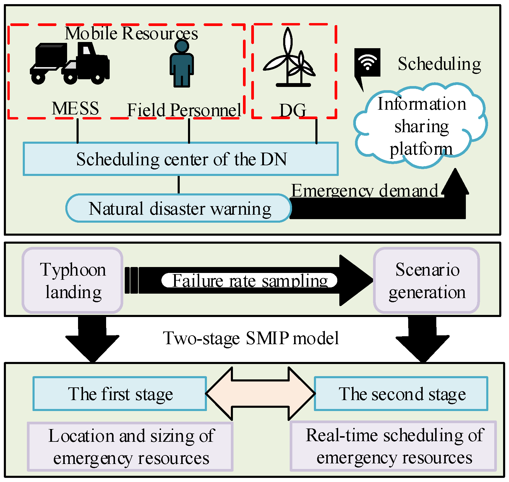
The proposed strategy for proactive scheduling of the DN with emergency resource participation is illustrated in Figure 1. Taking a typhoon as an example, the DN scheduling center obtains typhoon forecast information through an information-sharing platform and calculates the real-time fault probability of distribution lines. Multiple fault scenarios for the DN under typhoon conditions are generated through sampling. Based on fault scenarios, a two-stage SMIP model for pre-disaster and post-disaster emergency resource coordination and control is constructed. In the preventive response stage, the quantity and location of emergency resources such as MESSs, RCs, and SCs are determined. In the real-time restoration stage, emergency resources are dynamically scheduled according to the latest disaster conditions, and sequential restoration of the DN is realized by the coordinated efforts of multiple resources.
This paper focuses on a regional DN, whose relatively small scale implies that it will only be affected by the typhoon wind field for a limited time. When a typhoon passes through the DN, the probability of overhead line breakages and pole collapses increases. The anticipated faults in the DN are assumed to be caused by failures of these two components: overhead lines and poles. Based on pre-disaster meteorological forecast data, the typhoon path and wind speed can be obtained, allowing the estimation of the fault probability of conductors and poles under wind load influence. Under typhoon wind loads, both conductors and poles are subject to failure according to the stress–strength interference model [22]. The tensile strength of aluminum conductor steel-reinforced conductors and the bending strength of concrete poles, calculated from wind loads, both follow normal distributions. The failure rates of conductors and poles are given by Equations (1) and (2), respectively, while the overall failure rate of distribution line is given by Equation (3). The specific values of the means and standard deviations are provided in [22].
  λ l i n e = 0 σ g 1 2 π δ 1 exp 1 2 σ 1 μ 1 δ 1 2 d σ 1
λ t o w e r = 0 M T 1 2 π δ p exp 1 2 M p μ p δ p 2 d M p
λ l = 1 m = 1 M 1 1 λ l , m t o w e r m = 1 M 2 1 λ l , m l i n e

3. Logical Relationships of Line Operational States

3.1. RCs and Faulty Lines

In the TSN, depots, fault points, and the connecting arcs between them form the operational foundation for RCs. These arcs represent the possible movement routes for RCs. The TSN includes two main types of paths: movement arcs and docking arcs. Movement arcs facilitate the transportation of RCs between depots and fault points, while docking arcs allow RCs to pause at specific fault points to perform line repair tasks. Based on this network structure, an operational plan for RCs can be formulated within a specified time range, ensuring efficient scheduling between different locations. Equation (4) enforces single-action-per-period constraints for each RC; Equation (5) represents the balance of actions between consecutive time periods; Equation (6) specifies the initial location of RCs; Equation (7) imposes immediate return prohibitions for RCs arriving at fault sites; and Equation (8) ensures that RCs return to the initial temporary depot site.
  d p Ω x r c , d p R C / N R C   + 1 ( e , f ) Z R C ζ r c , e f , s , t d p Ω x r c , d p R C , r c R C , t T , s S
( e , f ) Z R C , e ζ r c , e f , s , t = ( e , f ) Z R C , e + ζ r c , e f , s , t + 1 , r c R C , e N R C N R C V , t T \ { T } , s S
  ( e , f ) Z R C , e + ζ r c , e f , s , 1 = ζ r c , e , s , 0 , r c R C , e N R C N R C V , s S
  ζ r c , e f , s , t + ζ r c , f e , s , t + 1 1 , r c R C , ( e , f ) Z R C , e f , t T \ { T } , s S
ζ r c , e , s , 0 = x r c , d p R C , r c R C , e N R C , s S
During the process of RCs repairing faulty lines, the lines can exist in three states: faulty, under repair, and operating. The transitions among these states are illustrated in Figure 2. It should be emphasized that the faulty state can switch to the under repair state at any time, but the under repair state typically requires a certain amount of time to complete. Therefore, this paper improves the multi-state operational model [23] as shown in (9)–(17). Constraint (9) demonstrates that a line is restricted to being in a single state at any specific instant; Constraint (10) defines the shortest time period that the state of being under repair must last, meaning that a line can enter the under repair state at most once and cannot leave this state within that time period; Constraint (11) represents the state transition relationship between consecutive time periods; Constraint (12) ensures that a line cannot simultaneously enter and leave the under repair state; Constraints (13)–(15) describe the relationship between the faulty/under repair/operating states of a line and its entry/exit from these states; Constraint (16) indicates that a line can only be put into service after it reaches the normal operation state; and Constraint (17) states that a line enters the under repair state after RCs arrive at the repair location.
η i j , s , t + μ i j , s , t + ξ i j , s , t = 1 , ( i , j ) L 0 , t T , s S
t = u u + N r c i j , m i n 1 I i j , s , t μ , i n 1 t = u u + N r c i j , m i n 1 ( I i j , s , t μ , i n + I i j , s , t μ , o u t ) 1 , 1 u | T | + 1 N r c i j , m i n , ( i , j ) L 0 , s S
I i j , s , t η , o u t = I i j , s , t μ , i n , I i j , s , t μ , o u t = I i j , s , t ξ , i n , ( i , j ) L 0 , t T , s S
I i j , s , t μ , i n + I i j , s , t μ , o u t 1 , ( i , j ) L 0 , t T , s S
I i j , s , t η , o u t = η i j , s , t η i j , s , t 1 , ( i , j ) L 0 , t T , s S
I i j , s , t μ , i n I i j , s , t μ , o u t = μ i j , s , t μ i j , s , t 1 , ( i , j ) L 0 , t T , s S
I i j , s , t ξ , i n = ξ i j , s , t ξ i j , s , t 1 , ( i , j ) L 0 , t T , s S
α i j , s , t ξ i j , s , t , ( i , j ) L 0 , t T , s S
μ i j , s , t = ζ r c , e e , s , t , e ( i , j ) , t T , s S

3.2. SCs and Line Switches

Similar to RCs, SCs are treated as mobile resources, with their temporary depot sites serving as departure points and the locations of line switches as docking points. The TSN is used to establish a scheduling model for SCs. Equation (18) enforces single-action-per-period constraints for SCs; Equation (19) represents the balance of actions between consecutive time periods for SCs; Equation (20) specifies the initial state of SCs; Equation (21) restricts SCs from immediately returning after arriving at a node; and Equation (22) ensures that SCs return to the initial site.
  d p Ω x s c , d p S C / N S C   + 1 ( e , f ) Z S C ζ s c , e f , s , t d p Ω x s c , d p S C , s c S C , t T , s S
( e , f ) Z S C , e ζ s c , e f , s , t = ( e , f ) Z S C , e + ζ s c , e f , s , t + 1 , s c S C , e N S C N S C V , t T \ { T } , s S
( e , f ) Z S C , e + ζ s c , e f , s , 1 = ζ s c , e , s , 0 , r c S C , e N S C N S C V , s S
ζ s c , e f , s , t + ζ s c , f e , s , t + 1 1 , s c S C , ( e , f ) Z S C , e f , t T \ { T } , s S
ζ s c , e , s , 0 = x s c , d p S C , r c S C , e N S C , s S
It is assumed that the switching time for line switches with remote control is negligible, and SCs only need to spend time operating line switches with manual control. During the process of SCs operating line switches, the switch states in the DN can exist in three states: open, acting, and closed. The possible transitions between these states are illustrated in Figure 3. It should be particularly noted that the open state and the closed state are capable of transitioning to the acting state at any moment, but the acting state typically requires a certain duration to complete. Therefore, this paper establishes a multi-state operational model, as shown in (23)–(29). Constraint (23) indicates that, at any specific point in time, a line switch is restricted to being in just one state; Constraint (24) sets out the minimum time length that the acting state should maintain, meaning that a line switch can enter the acting state at most once and cannot leave this state within that time period; Constraint (25) embodies the relationship of state transformation across successive time intervals; Constraint (26) guarantees that a line switch is prohibited from both entering and exiting state h at the same time; Constraint (27) depicts the connection between state h of a line switch and its entry/exit from this state; Constraint (28) states that a line switch transitions to the acting state after SCs arrive at the line; and Constraint (29) indicates that a line switch enters the normal operation state after being closed.
k = 1 3 x i j , s , t s w , h = 1 , ( i , j ) L S W , t T , s S , h 1 , 2 , 3
t = u u + N s c i j , m i n 1 I i j , s , t s w , 2 , i n 1 t = u u + N s c i j , m i n 1 ( I i j , s , t s w , 2 , i n + I i j , s , t s w , 2 , o u t ) 1 , 1 u | T | + 1 N s c i j , m i n , ( i , j ) L S W , s S
I i j , s , t s w , 1 , o u t + I i j , s , t s w , 3 , o u t = I i j , s , t s w , 2 , i n , I i j , s , t s w , 1 , i n + I i j , s , t s w , 3 , i n = I i j , s , t s w , 2 , o u t , ( i , j ) L S W , t T , s S
I i j , s , t s w , h , i n + I i j , s , t s w , h , o u t 1 , ( i , j ) L S W , t T , s S , h 1 , 2 , 3
I i j , s , t s w , h , i n + I i j , s , t s w , h , o u t = x i j , s , t s w , h x i j , s , t 1 s w , h , ( i , j ) L S W , t T , s S , h 1 , 2 , 3
x i j , s , t s w , 2 = ζ s c , e e , s , t , e ( i , j ) , t T , s S
x i j , s , t s w , 3 = α i j , s , t , ( i , j ) L S W , t T , s S

4. Two-Stage SMIP Model

4.1. Objective Function

The objective function for emergency resources participating in the proactive scheduling of the DN aims to minimize the pre-disaster pre-scheduling costs and the real-time operational costs of MESSs, RCs, and SCs, as shown in (30). The actual operational cost of the DN under scenario s includes the operational costs of MESSs, RCs, and SCs, as well as the load shedding cost, as shown in (31)–(35).
min c m e s s ω M E e N M E x ω , e M E S S + c r c d p Ω r c R C x r c , d p R C + c s c d p Ω s c S C x s c , d p S C + s S p ( s ) ϕ ( s )
ϕ ( s ) = C s M E S S + C s R C + C s S C + C s D
C s M E S S = t T ω M E c ω t r a n ( e , f ) Z M E , e f ζ ω , e f , s , t
C s R C = t T r c R C c r c t r a n ( e , f ) Z R C , e f ζ r c , e f , s , t
C s S C = t T r c S C c s c t r a n ( e , f ) Z S C , e f ζ s c , e f , s , t
C s D = t T i N c i d P i , s , t c Δ t

4.2. Constraints

Constraints (36)–(38) limit the maximum number of schedulable MESSs, RCs, and SCs, respectively.
ω M E e N M E x ω , e M E S S N M E S S
r c R C d p Ω x r c , d p R C N R C  
s c S C d p Ω x s c , d p S C N S C  
The operational constraints of MESSs are similar to those of traditional energy storage facilities, including output power constraints and state of charge (SOC) constraints, as shown in (39)–(47). Specifically, Constraints (39)–(42) define the feasible range of MESS charging and discharging power; Constraints (43) and (44) ensure that MESS cannot charge and discharge simultaneously; Constraint (45) restricts the operational mode of MESS, indicating that MESS is only allowed to charge or discharge when docked at an energy storage station; and Constraints (46) and (47) represent the SOC constraints for MESSs.
0 P ω , e , s , t c h ζ ω , e e , s , t P eq M E S S , ω M E , e N M E , t T , s S
0 P ω , e , s , t d i s ζ ω , e e , s , t P eq M E S S , ω M E , e N M E , t T , s S
θ P ω , e , s , t c h Q ω , e , s , t c h θ P ω , e , s , t c h , ω M E , e N M E , t T , s S
θ P ω , e , s , t d i s Q ω , e , s , t d i s θ P ω , e , s , t d i s , ω M E , e N M E , t T , s S
  0 e N M E P ω , e , s , t c h I ω , s , t c h P eq M E S S , ω M E , t T , s S
  0 e N M E P ω , e , s , t d i s I ω , s , t d i s P eq M E S S , ω M E , t T , s S
I ω , s , t c h + I ω , s , t d i s e N M E ζ ω , e e , s , t , ω M E , t T , s S
E ω , s , t + 1 M E S S = E ω , s , t M E S S e N E P ω , e , s , t + 1 d i s η ω d i s η ω c h e N E P ω , e , s , t + 1 c h Δ T , ω M E , t T \ { T } , s S
S O C min E eq M E S S e N M E x ω , e M E S S E ω , s , t M E S S S O C max E eq M E S S e N E x ω , e M E S S , ω M E , t T , s S
Constraints (48)–(51) represent the power balance constraints; Constraint (52) represents the line transmission capacity constraint; Constraints (53) and (54) represent the load shedding constraints; Constraints (55)–(57) represent the voltage constraints; and Constraints (58) sets the upper and lower limits for the output of distributed generations (DGs). Constraints related to network reconfiguration and node energization can be found in [24], which provides detailed guidelines and limitations, ensuring that network reconfiguration and node energization are carried out safely and effectively.
( j , k ) L P j k , s , t ( i , j ) L P i j , s , t = P j , s , t I N ( P j , s , t d P j , s , t c ) , j N , t T , s S
( j , k ) L Q j k , s , t ( i , j ) L Q i j , s , t = Q j , s , t I N ( Q j , s , t d Q j , s , t c ) , j N , t T , s S
P j , s , t I N = P j , s , t d g + ω Ω P ω , j , s , t d i s ω Ω P ω , j , s , t c h , j N , t T , s S
  Q j , s , t I N = Q j , s , t d g + ω Ω Q ω , j , s , t d i s ω Ω Q ω , j , s , t c h , j N , t T , s S
P i j , s , t 2 + Q i j , s , t 2 α i j , s , t S i j max , ( i , j ) L , t T , s S
0 P i , s , t c P i , s , t d , i N , t T , s S
Q i , s , t c = P i , s , t c × tan φ i , i N , t T , s S
V i , s , t V j , s , t 2 r i j P i j , s , t + x i j Q i j , s , t + α i j , s , t 1 M , ( i , j ) L , t T , s S
V i , s , t V j , s , t 2 r i j P i j , s , t + x i j Q i j , s , t + 1 α i j , s , t M , ( i , j ) L , t T , s S
V i min V i , s , t V i max , i N , t T , s S
0 P i , s , t d g P i , max d g , 0 Q i , s , t d g Q i , max d g , i N G , t T , s S

4.3. Model-Solving Approach

The analysis shows that the proposed two-stage optimization model for emergency resources in both pre-disaster and post-disaster situations is, in essence, a two-stage SMIP model. The established two-stage SMIP model can be formulated as presented in (59)–(62):
min x c T x + s S p ( s ) f ( x , s )
s . t .   A x b
  f ( x , s ) = min g T y
  s . t .   W y r ( s ) T ( s ) x
Similar to [24], this paper considers uncertainties in load levels, fault line locations, line repair times, and DG output uncertainty. Since this paper focuses on extreme weather scenarios exemplified by typhoons, the line failure rates are not directly derived from statistical data, but are calculated based on simulations of the typhoon disaster process to obtain time-varying failure rates for faulty lines. Based on this, several fault scenarios are selected as samples, and representative and typical scenarios are derived by means of scenario generation and simplification. First, operation scenarios are generated considering the uncertainty of fault locations, load levels, and repair times. Then, the scenarios that greatly affect SMIP are identified and minimized. Finally, the k-means clustering method is used to obtain typical representative scenarios. Ultimately, the progressive hedging algorithm (PHA) is utilized to solve the model. More detailed steps are provided in Appendix A.

5. Case Study

The case study was tested on a computer with an Intel Core i5-8400 processor and 16 GB of RAM. The model was programmed using the YALMIP toolbox in MATLAB R2024a, and the Gurobi 10.0.1 solver was used to generate a solution.

5.1. Results of the Experiments on an IEEE 33-Node System

(1) Scenario Generation and Reduction
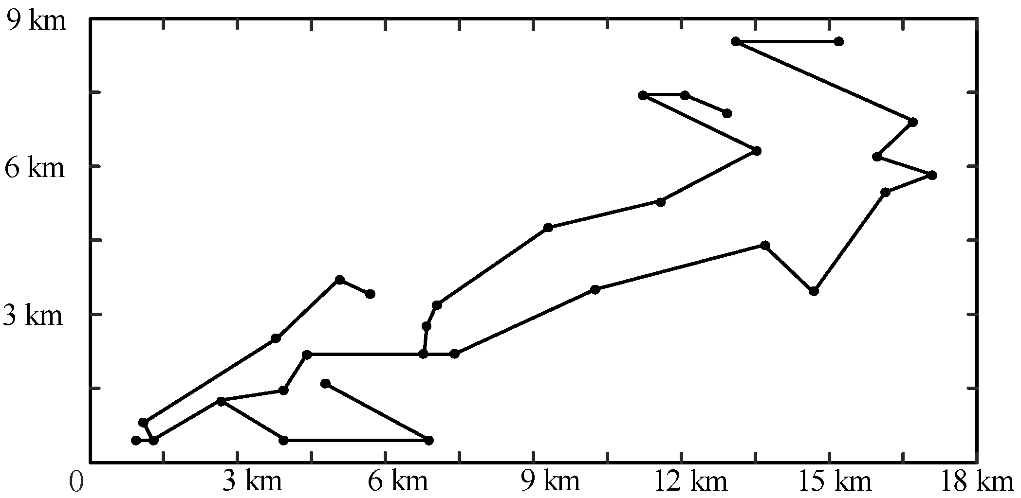
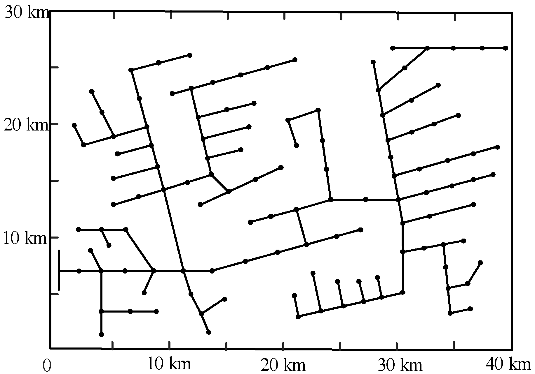
In order to verify the efficacy of the suggested model, the IEEE 33-node system was employed. This region is close to the coastline and frequently experiences extreme weather such as typhoons during summer and autumn. The basic design wind speed for distribution lines is 25 m/s, and the geographical layout of the feeders is consistent with Figure 4 [22]. The average span length of the overhead lines is 50 m. It is assumed that the typhoon makes landfall at coordinates −125 km, −150 km and moves at a speed of 20 km/h at a 45° angle to the horizontal axis. Other parameters are consistent with those in [24].
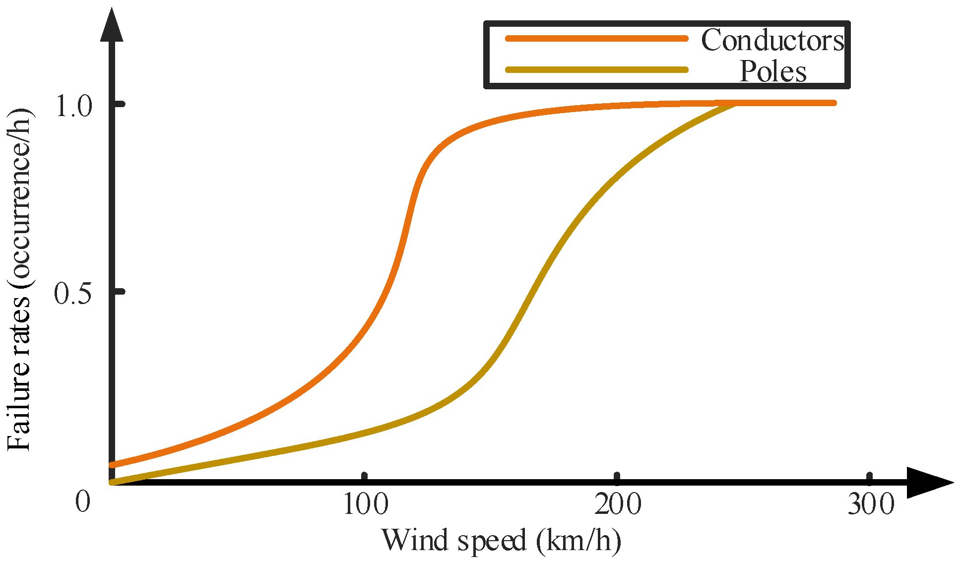
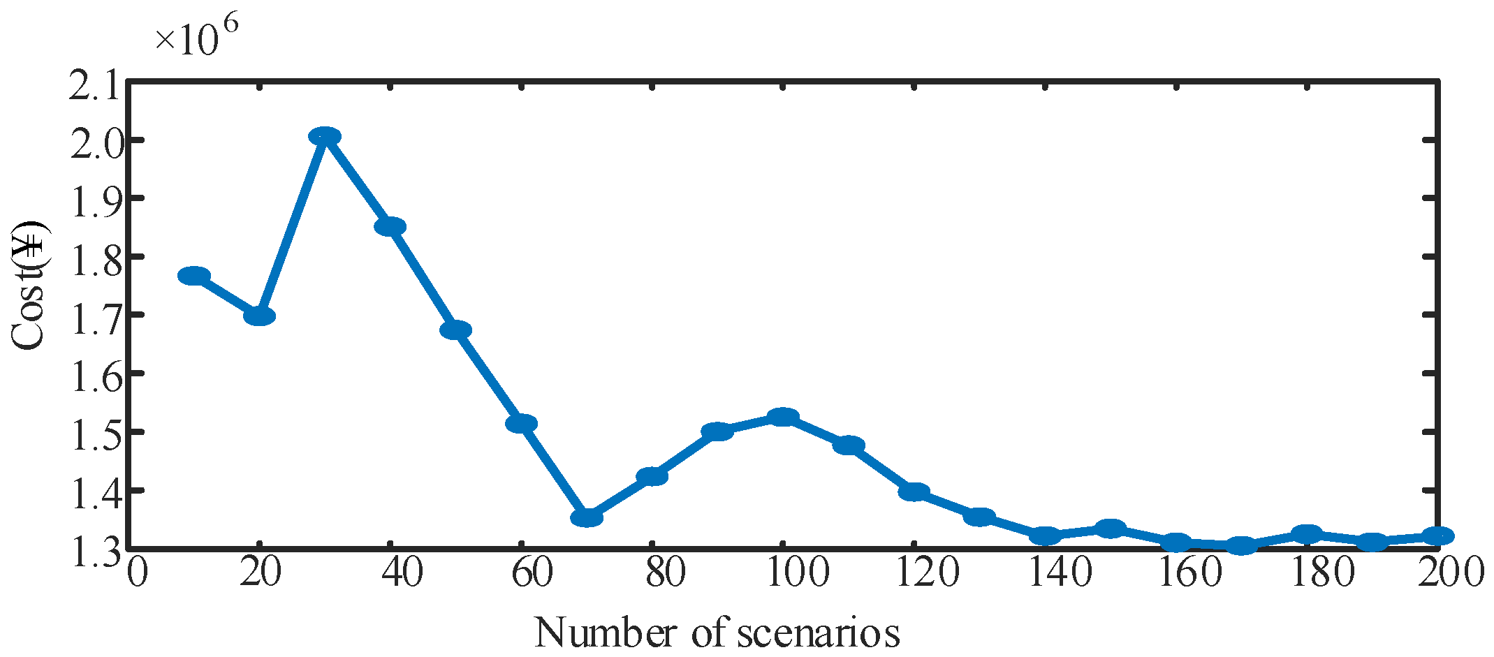
According to the wind field information, the correlation between the failure rates of the DN components and the wind speed is obtained, as illustrated in Figure 5. It is evident that, once the wind speed surpasses 120 km/h, there is a notable increase in the failure rates of both conductors and towers. As the typhoon approaches, the wind speed along the lines gradually increases. By calculating the time-varying failure rate of distribution lines, it can be found that, during the typhoon, the failure rates of distribution lines are high, making faults highly likely. We generate the failure rate and repair time of each distribution line through random sampling based on historical statistics [21]. This paper randomly sampled 200 typhoon weather scenarios, with the average cost shown in Figure 6. Once the number of scenarios reaches 140, the average cost for extreme scenarios becomes stable and remains around ¥1,320,000. The threshold of the minimum cost during typhoon season is ¥100,000, and 115 fault scenarios are chosen. These 115 fault scenarios are clustered and reduced, resulting in the selection of 45 representative fault scenarios.
(2) Scheduling Results
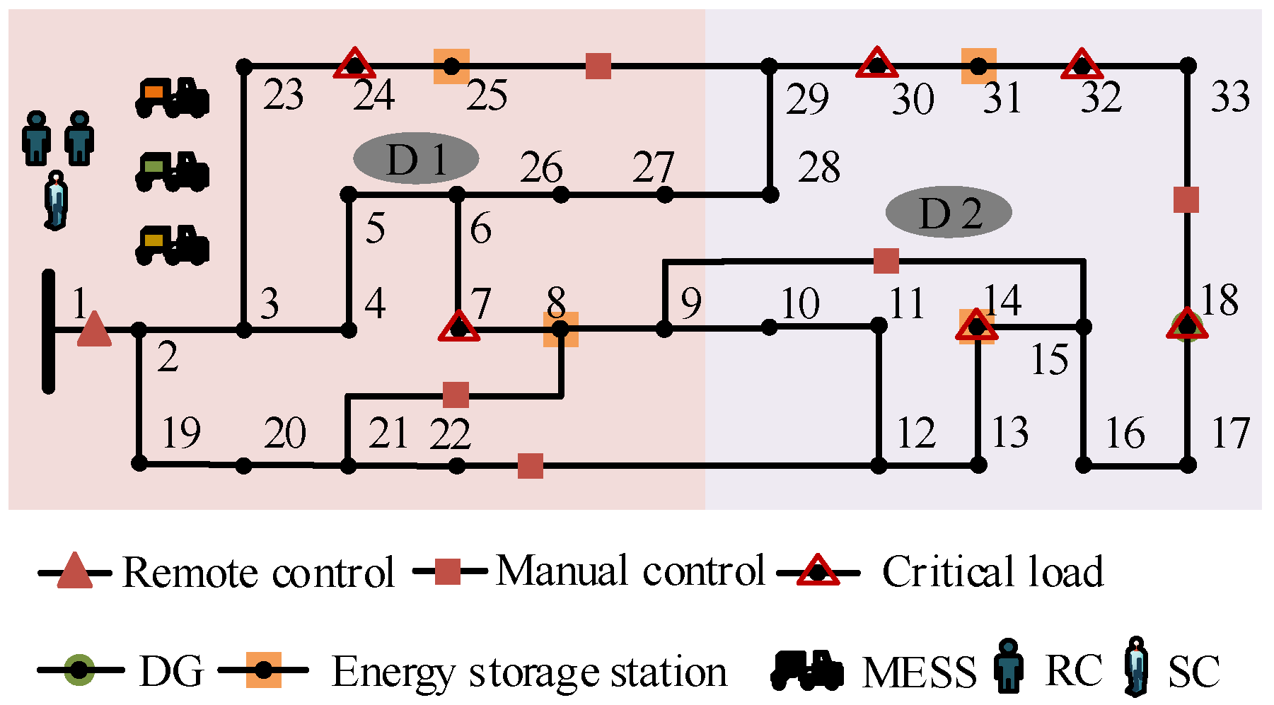
The IEEE 33-node system, after being modified, is presented in Figure 7. It is presumed that there are three MESSs, two RCs, and one SC available for pre-scheduling. The DN includes one DG at node-18, one remotely controlled switch, and five manually operated switches. The opening and closing time of the remotely controlled switch is assumed to be negligible, while the operation time of the manually operated switches is 10 min. Before the disaster, the DN is divided into two regions based on geographical location, with temporary stations established at D1 and D2. The assignment of RCs and SCs to each station is to be determined. It is assumed that travel time within the same region is 10 min, while travel time across regions is 30 min. The cost of pre-scheduling an RC/SC to a station is assumed to be ¥300. The MESSs are specified to have a rated power of 1000 kW and a capacity of 1000 kW·h, and the efficiency for charging as well as discharging is 0.9 in each case. The SOC limits are between 0.05 and 0.95. MESSs are capable of being linked to energy storage stations situated at nodes 2, 15, 22, and 31. The unit time is set to 10 min, and for each unit of this time period the transportation cost for MESSs, RCs, and SCs is ¥10.
The penalty factor ρ applied in PHA is set to 280, and this value is marginally lower than the cost of scheduling a RC to a station. After 28 iterations, the computation time is 78 min, and the pre-scheduling results are obtained. Before the disaster, one RC and one SC are scheduled to D2, one RC is scheduled to D1, and MESSs are scheduled to nodes 8, 25, and 31, respectively. The solution results of the model are shown in Case 4 of Table 1. The expected load shedding loss of the DN is ¥45,773. By coordinating and controlling emergency resources for pre-disaster scheduling and post-disaster restoration, the load shedding loss can be effectively reduced, the restoration process improved, and the operational costs of the DN minimized.
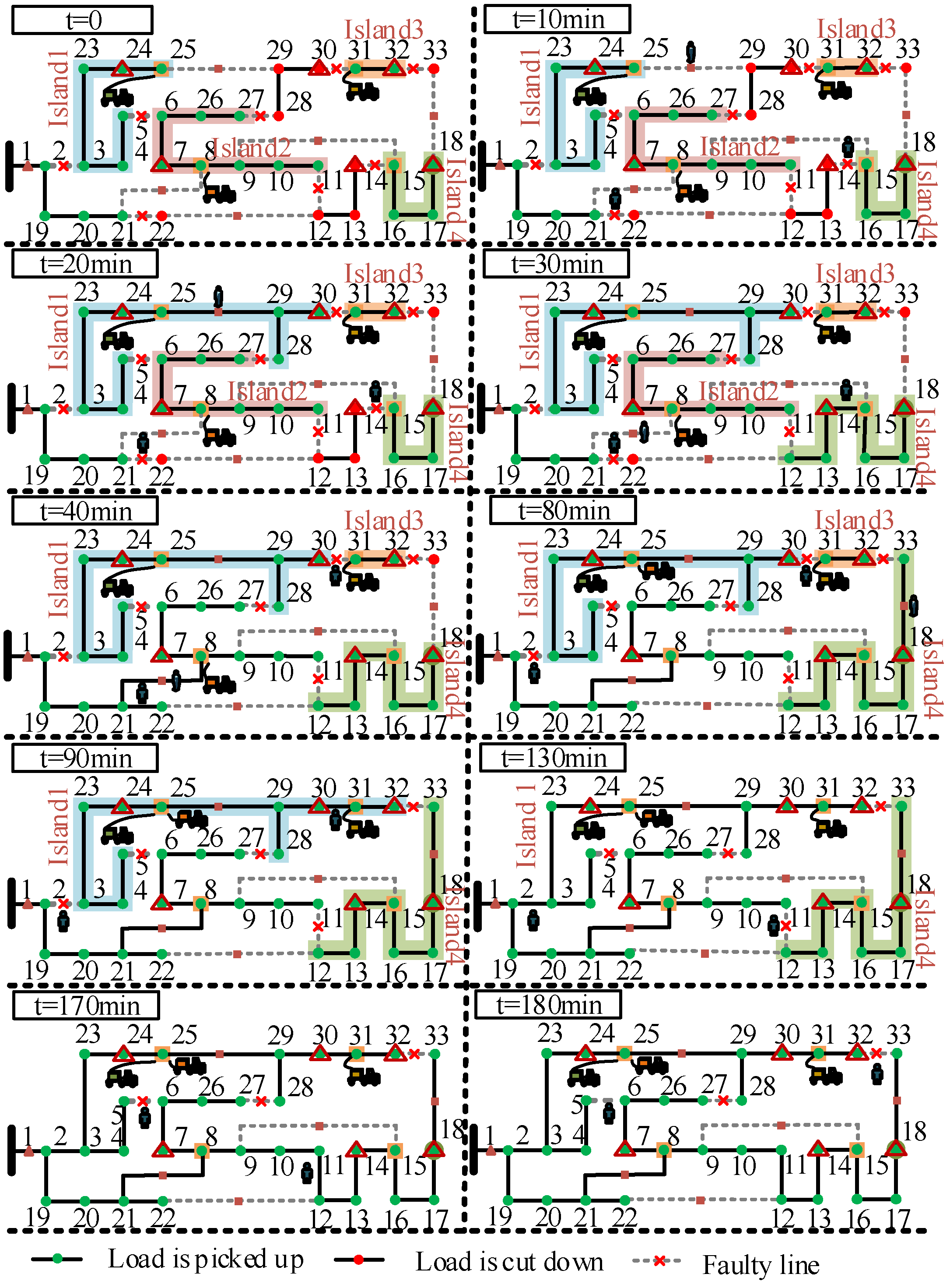
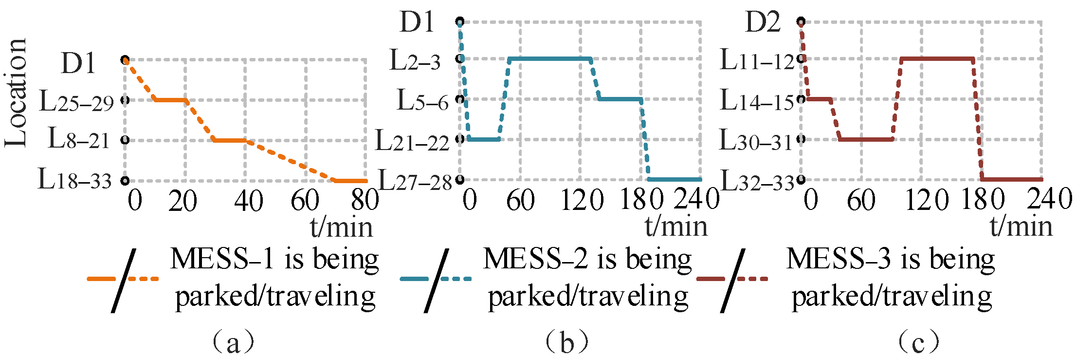
As shown in Figure 8 and Figure 9, protective actions are triggered after faults occur on eight lines (L2–3, L5–6, L11–12, L14–15, L21–22, L27–28, L30–31, and L32–33), and the remote switch at L1–2 opens to isolate the faults in fault scenario 3. At the beginning of fault recovery, the DN shares the operational status of all lines and initiates the restoration process. At t = 0, the remote switch at L1–2 closes, while other faulty lines are taken out of service. The loads at nodes 2, 19, 20, and 21 are supplied by the main grid. The network is partitioned into four separate islands: in Island 1, the loads at nodes 3, 4, 5, 23, 24, and 25 are supported by MESS-1 located at node 25; in Island 2, the loads at nodes 6, 7, 8, 9, 10, 11, 26, and 27 are supported by MESS-2 located at node 8; in Island 3, the loads at nodes 31 and 32 are supported by MESS-3 located at node 31; in Island 4, the loads at nodes 15, 16, 17, and 18 are supported by the DG located at node 18. Due to line outages, the loads at nodes 12, 13, 14, 22, 28, 29, and 30 are shed. Meanwhile, RCs are dispatched to repair L21–22 and L14–15, while SCs are dispatched to L25–29 to perform switching operations for network reconfiguration.
At t = 10 min, RC-1 and RC-2 arrive at L21–22 and L14–15, respectively, to begin line repair work. Meanwhile, the SC arrives at L25–29 to prepare for manual switch closure. At t = 20 min, the SC completes the closure of the switch at L25–29. After the line is closed and enters operational status, it participates in network reconfiguration. Island 1 can continue to support the loads at nodes 28, 29, and 30. The SC is then dispatched to L8–21 for further switching operations. At t = 30 min, the SC arrives at L8–21 to prepare for manual switch closure. Meanwhile, RC-2 completes the repair of L14–15, and the line is put back into operation. Island 4 supports the loads at nodes 12, 13, and 14. RC-2 is then dispatched to L30–31 for further repairs. At t = 40 min, RC-1 completes the repair of L21–22, and the load at node 22 is restored. RC-1 is then dispatched to L2–3 to begin repairs. Meanwhile, the SC closes the switch at L8–21, connecting Island 2 to the main grid. This is because the capacity of the MESS is limited and cannot support the island for an extended period. At t = 50 min, MESS-2 arrives at the energy storage station at node 25 and works together with MESS-1 to support the loads in Island 1. At t = 70 min, the SC arrives at L18–33 to close the switch. At t = 80 min, RC-1 is repairing L2–3, and the SC successfully closes the switch at L18–33. Island 4 supports the load at node 33, and all loads in the DN are restored at this point. At t = 90 min, RC-2 completes the repair of L30–31. Island 1, supported by all three MESS units, supplies power to the loads at nodes 3, 4, 5, 23, 24, 25, 28, 29, 30, 31, and 32. At t = 130 min, RC-1 completes the repair of L2–3, and the line is put back into operation. Island 1 is reconnected to the main grid. At t = 170 min, RC-2 completes the repair of L11–12, and the line is returned to operation. Island 4 is reconnected to the main grid. At t = 180 min, RC-2 arrives at L32–33 to begin repairs. At t = 240 min, all lines are fully repaired, and the load shedding loss for this scenario is ¥61,929.
(3) Comparison Among Distinct Cases
Case 1: Only pre-scheduling RCs and SCs, without using MESSs [25].
Case 2: All faulty lines are uniformly restored before deployment, with only MESSs pre-scheduled for emergency response [26].
Case 3: The pre-scheduling results of RCs and SCs are fixed first, with MESSs then comprehensively scheduled on this basis [27].
Case 4: The proposed method in this paper, which integrates the pre-scheduling of MESSs, RCs, and SCs.
The comparison results of the cases are shown in Table 2. In Case 1, only repair crews and switching crews are pre-scheduled, without considering mobile energy storage. Due to the lack of emergency power support, critical loads experience sustained outages during repairs, resulting in the highest load shedding cost of ¥516,487 among all cases.
In Case 2, although MESSs are pre-scheduled, all faulty lines must be fully repaired by RCs before MESSs can be uniformly put into service. During the repair period, MESSs are unable to support critical loads in a timely manner, leading to a load shedding cost of ¥175,644, significantly higher than that of our method.
In Case 3, the repair and switching plans are fixed first, and MESSs are then scheduled on this basis. This improves over the first two cases, reducing the shedding cost to ¥56,524. However, since MESSs are only passively adapted in the second stage, without tight real-time coordination with repair and switching operations, there remains room for improvement.
The proposed coordinated restoration method, i.e., Case 4, simultaneously dispatches MESSs, RCs, and SCs in a synchronized manner. MESSs dynamically moves according to restoration status and cooperates with network reconfiguration, while repair and switching crews operate in coordination with fault repair and switching timing requirements. This achieves tight spatiotemporal coordination of multiple resources, reducing the load shedding cost to ¥45,773—representing reductions of 91.1%, 73.9%, and 19.0% compared to Cases 1, 2, and 3, respectively—demonstrating the effectiveness of the proposed model in enhancing post-disaster recovery efficiency.

5.2. Results of the Experiments on an IEEE 123-Node System

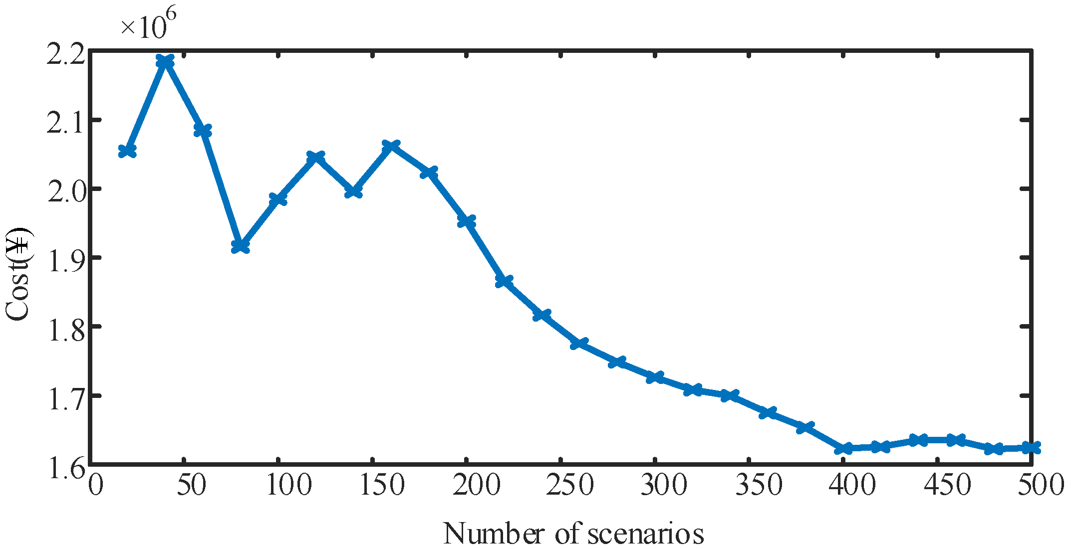
In an effort to authenticate the scalability of the proposed model, this paper undertakes supplementary tests on an extended-scale IEEE 123-node system. The precise data associated with the test system are congruent with the content documented in [21]. Based on the IEEE 33-node system and referencing an actual DN region near the coastline, the geographical layout of its feeders is consistent with Figure 10 [25]. The typhoon landing location and wind speed parameters remain unchanged. After calculating the failure rates of each line, fault scenarios are generated through sampling. As shown in Figure 11, once the number of scenarios hits 400, the average cost for extreme scenarios becomes stable and remains around ¥1,620,000. Similarly, the threshold of the lowest cost for fault situations is determined to be ¥100,000, and a total of 163 fault scenarios are chosen. On the basis of these selections, 75 typical fault scenarios are highlighted specifically for extreme weather.
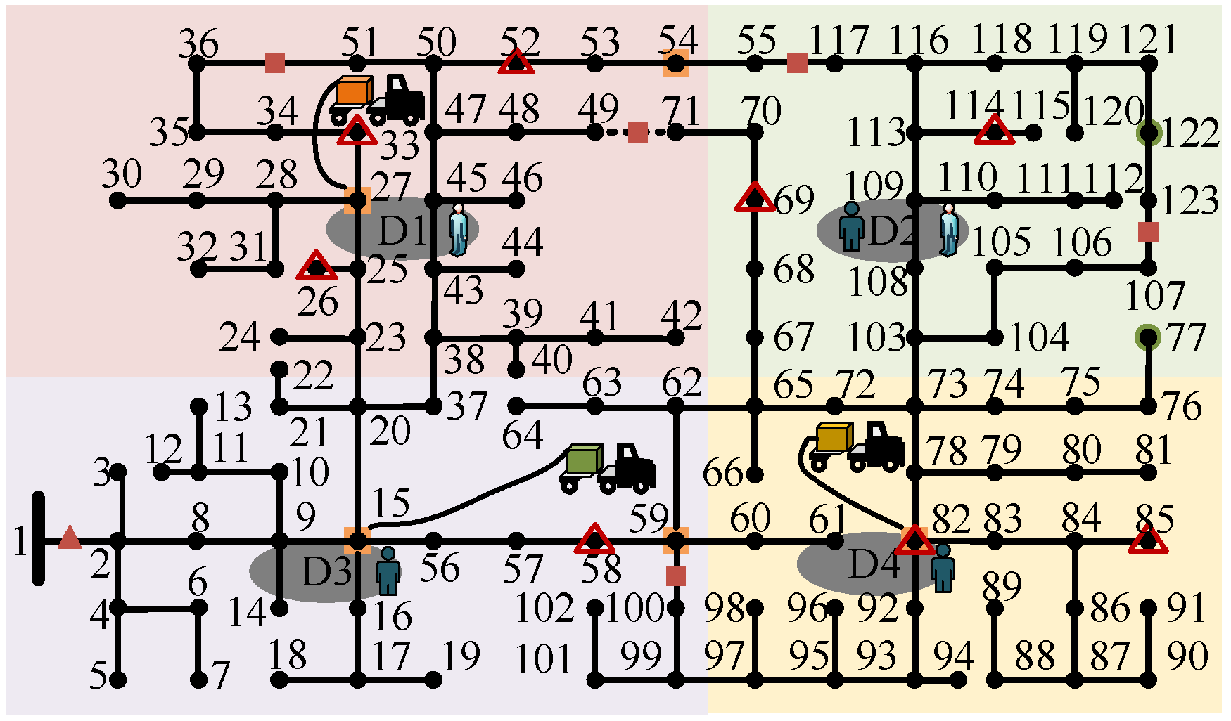
It is assumed that there are three MESSs, three RCs, and two SCs available for pre-scheduling. The DN includes two DG, one remotely controlled switch, and five manually operated switches. Before the disaster, the DN is divided into four regions based on geographical location, and temporary stations are established in each region. The number of RCs and SCs at each station is to be determined. It is assumed that the travel time for MESSs, RCs, and SCs within the same region is 10 min, while the travel time between different regions is 40 min. MESSs are capable of being linked to energy storage stations situated at nodes 15, 27, 54, 59, and 82. Having carried out 49 iterations and consumed 8.6 h for the calculation, we obtain the pre-scheduling results that are depicted in Figure 12. Before the disaster, one SC is scheduled to D1, one RC and one SC are scheduled to D2, one RC is scheduled to D3, and one RC is scheduled to D4. The three MESSs are scheduled to nodes 15, 27, and 82, respectively.
The comparison of Cases 1–4 in the IEEE 123-node system are presented in Table 3. The overall trend is consistent with that of the 33-node system. In Case 1, the load shedding cost reaches the highest value of ¥961,325 due to the absence of MESSs. In Case 2, although MESSs are pre-scheduled, they cannot be put into service until all faulty lines are fully repaired by RCs, resulting in a shedding cost of ¥274,614. In Case 3, MESSs are introduced on the basis of fixed RC and SC pre-scheduling, reducing the cost to ¥73,684. In Case 4, the proposed coordinated scheduling strategy simultaneously dispatches MESSs, RCs, and SCs, reducing the load shedding cost to ¥48,953, further validating the effectiveness of the proposed method in large-scale systems.
The solution times of the proposed model for both the 33-node and 123-node systems are far less than the typical typhoon warning lead time (24–72 h), demonstrating sufficient engineering practicality. Moreover, leveraging the warm-start capability of PHA and a hierarchical decision-making strategy, the model can effectively handle periodic forecast updates, ensuring timely scheduling decisions under dynamic meteorological conditions, which is of practical engineering significance. However, this paper assumes fixed travel times for RCs and SCs without considering road network damage during typhoons and major storms, and in future work we will introduce stochastic travel time models or real-time traffic-aware dynamic routing to address this issue.

6. Conclusions

To further enhance the proactive response capability of emergency resources to disasters and strengthen recovery efficiency and stability during disasters, this paper delves into how to comprehensively and efficiently improve restoration of the DN. Innovatively, a two-stage SMIP model integrating MESSs, RCs, and SCs is proposed. This model fully considers the reasonable allocation and coordinated operation of emergency resources in complex and variable disaster environments, aiming to achieve optimal configuration and efficient utilization of emergency resources. The model put forward in this paper is verified on standard IEEE test systems. The simulation results demonstrate that the model can achieve sequential restoration of the DN through reasonable pre-disaster preparation. Specifically, the load shedding cost of the proposed method (Case 4) is reduced by 19.0% compared to Case 3 in the 33-node system and by 19.9% in the 123-node system, fully validating the significant improvement of the proposed model in terms of load restoration performance across different system scales and enabling the DN to proactively respond to extreme disasters in a more resilient manner.

Author Contributions

Conceptualization, H.C.; methodology, H.C.; software, H.C.; validation, H.C. and Q.L.; formal analysis, H.C. and Q.L.; investigation, H.C.; resources, H.C. and Q.L.; data curation, H.C.; writing—original draft preparation, H.C.; writing—review and editing, Q.L.; visualization, H.C. and Q.L.; supervision, Q.L.; project administration, Q.L.; funding acquisition, Q.L. All authors have read and agreed to the published version of the manuscript.

Funding

This study was supported by the scientific and technological program from the Electric Power Research Institute of State Grid Chongqing Electric Power Company (Grant No: 2026 Chongqing Electric S&T No.6).

Data Availability Statement

The original contributions presented in this study are included in the article. Further inquiries can be directed to the corresponding author.

Acknowledgments

The authors appreciate the support provided by the Electric Power Research Institute of State Grid Chongqing Electric Power Company in carrying out this work.

Conflicts of Interest

Hongzhou Chen and Qinglong Liao are employees of the Electric Power Research Institute of State Grid Chongqing Electric Power Company. The authors declare that the research was conducted in the absence of any commercial or financial relationships that could be construed as potential conflicts of interest. This research was funded by the scientific and technological program of State Grid Chongqing Electric Power Company (Grant No. 2026 Chongqing Electric S&T No. 6). The funder was not involved in the study design; the data collection, analysis, or interpretation; the writing of the manuscript; or the decision to submit the manuscript for publication.

Nomenclature

A. Sets and Matrices
L / L 0 / L S W Set of distribution lines/faulty lines/line switches, indexed by (i, j)
N / N G Set of nodes/DGs, indexed by i, j, k
N M E Set of energy storage stations, indexed by e, f
N R C / N S C Set of locations of RCs/SCs, indexed by e, f
N R C V / N S C V Set of virtual locations of RCs/SCs
S Set of scenarios, indexed by s
T Set of time intervals, indexed by t
Ω Set of depots, indexed by dp
Z R C / Z S C Set of arcs of RCs/SCs in a TSN, indexed by (e, f)
Z M C , e + / Z M C , e Set of arcs starting/ending from location e of RCs in a TSN
Z S C , e + / Z S C , e Set of arcs starting/ending from location e of SCs in a TSN
ME/RC/SCSet of MESSs/RCs/SCs, indexed by ω/rc/sc
xVector of first-stage decisions that must be made before the scenario is known
y/c/A/b/g/WSMIP data
B. Parameters
μ l / δ l Mean/standard deviation of stress strength for overhead conductors
μ p / δ p Mean/standard deviation of bending strength for pole towers
M 1 / M 2 Number of poles/conductor spans for distribution line
η ω c h / η ω d i s Efficiency of charging/discharging of MESS ω
θ Power factor of MESSs
c i d Load shedding cost at node i
c m e s s / c r c / c s c Pre-scheduling cost of MESS ω/RC rc/SC sc
c ω t r a n / c r c t r a n / c s c t r a n Transportation cost per unit of MESS ω/RC rc/SC sc
φ i The average angle of the power factor of the load at node i
M A large constant
N M E S S / N R C / N S C Maximum number of pre-schedulable MESSs/RCs/SCs
N r c i j , m i n / N s c i j , m i n Minimum time required for RCs/SCs to repair/act on line (i, j)
p ( s ) The probability for the occurrence of scenario s
P eq M E S S / E eq M E S S Power/capacity rating of MESSs
r i j / x i j Resistance/reactance of line (i, j)
S i j max Apparent power rating of line (i, j)
S O C min / S O C max The smallest/largest permitted states of charge for MESSs
P i , max d g / Q i , max d g Maximum allowable value of active/reactive power of DGs at node i
Δ t The extent of a single temporal interval
C. Variables
λ l i n e / λ t o w e r Failure rate of overhead conductors/pole towers
σ l / M p Bending moment on overhead conductors/pole towers
λ l , m t o w e r / λ l , m l i n e Failure rate of pole/conductor m of line l
λ l Failure rate of line l
ϕ ( s ) Total annual operation cost of the DN
C s D Cost of load shedding in scenario s
C s M E S S MESS running cost in scenario s
C s R C / C s S C RC/SC running cost in scenario s
ζ ω , e f , t Binary variable activated when MESS ω is positioned on arc (e, f) during time t in scenario s
ζ r c , e f , s , t / ζ s c , e f , s , t Binary variable activated when RC rc/SC sc are positioned on arc (e, f) during time t in scenario s
P i , s , t c / Q i , s , t c Shedding of active/reactive loads at node i during time t in scenario s
V i , s , t The square value of the voltage magnitude at node i during time t in scenario s
V i min / V i max The square value of smallest/largest limit of the allowable voltage magnitude at node i
x ω , e M E S S Binary variable activated when MESS ω is pre-scheduled to station e
x r c , d p R C / x s c , d p S C Binary variable activated when RC rc/SC sc are pre-scheduled to depot dp
α i j , s , t Binary variable activated when line (i, j) is closed during time t in scenario s
η i j , s , t / μ i j , s , t / ξ i j , s , t Binary variable activated when line (i, j) is faulty/under repair/operating during time t in scenario s
I i j , s , t η , o u t Binary variable activated when line (i, j) exits the faulty state at the termination of time t in scenario s
I i j , s , t μ , i n / I i j , s , t μ , o u t Binary variable activated when line (i, j) enters/exits the under repair state at the termination of time t in scenario s
I i j , s , t ξ , i n Binary variable activated when line (i, j) enters the operating state at the termination of time t in scenario s
x i j , s , t s w , h Binary variable activated when the switch on line (i, j) is in h state at the termination of time t in scenario s (when h is 1/2/3, it corresponds to the open/acting/closed state)
I i j , s , t s w , h , i n / I i j , s , t s w , h , o u t Binary variable activated when line (i, j) enters/exits state h at the termination of time t in scenario s
L i j , s , t Current flowing through line (i, j) during time t in scenario s
E ω , s , t M E S S Amount of energy of MESS ω at the termination of time t in scenario s
P ω , e , s , t c h / P ω , e , s , t d i s Active power for charging/discharging of MESS ω positioned at station e during time t in scenario s
P i j , s , t / Q i j , s , t Flows of active/reactive power originating from node i to j during time t in scenario s
P i , s , t d g / Q i , s , t d g Output values of active/reactive power for DGs at node i during time t in scenario s
P i , s , t I N / Q i , s , t I N Active/reactive power input at node i during time t in scenario s
Q ω , e , s , t c h / Q ω , e , s , t d i s Reactive power for charging/discharging of MESS ω positioned at station e during time t in scenario s
I ω , s , t c h / I ω , s , t d i s Binary variable activated when MESS ω engages in charging/discharging activities during time t in scenario s

Appendix A

A direct invocation of a solver may not be sufficient to efficiently solve a two-stage stochastic programming model, which is generally a large-scale SMIP model. Once the selection of Ns scenarios is made, the problem can be expressed as
min s S p ( s ) c T x + g T y ( s ) : ( x ( s ) , y ( s ) ) K ( s ) , s S , x ( 1 ) = = x N s + s S p ( s ) ϕ ( s )
where K ( s ) = ( x , y ( s ) ) : A x b , W y r ( s ) T ( s ) x . Here, x ( 1 ) = = x N s represents the non-anticipative constraint. Finally, the scenario from (A1) decomposes the large-scale SMIP model into scenario subproblems with non-anticipative constraints. The PHA is employed to tackle the large-scale SMIP model given the uncertainty of multiple scenarios, as explained in [19]. The steps are as expressed as
1: k = 0, w k ( s ) = 0 . For all s ∈ S, x k + 1 ( s ) = argmin c T x + g T y ( s )
2: k = k + 1
3: x ¯ k ( s ) = s S p ( s ) x k ( s )
4: w k ( s ) = w k 1 ( s ) + ρ ( x k ( s ) x ¯ k ( s ) )
5: For all s ∈ S, x k + 1 ( s ) = argmin c T x + g T y ( s ) + w k ( s ) x + ρ 2 ( x x ¯ k ( s ) 2
6: g k = s S p ( s ) x k ( s ) x ¯ k ( s )
7: if g ( k ) < ϵ , where ϵ is the termination threshold, then go to Step 2.
Otherwise, terminate.
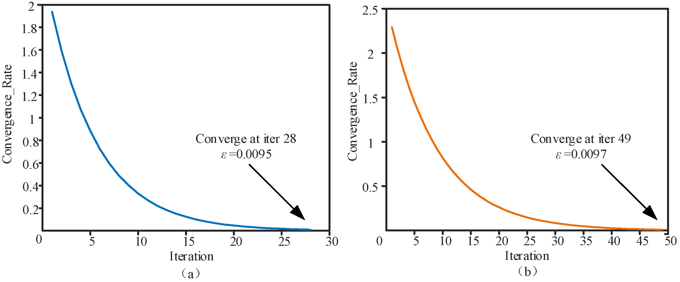
The size of ρ in the PHA directly affects the convergence and solution speed of the model [21]. The penalty factor ρ applied in PHA is set to 280, and this value is marginally lower than the cost of scheduling an RC to a station. The size of ε in the PHA is set to 0.01.
Figure A1. Convergence performance of the PHA. (a) IEEE 33-node system, (b) IEEE 123-node system.
Energies 19 04110 g0a1
Both curves exhibit the characteristic exponential decay profile of the PHA: the convergence rate drops sharply within the first ten iterations and then gradually levels off, ultimately plateauing below the prescribed tolerance, as illustrated in Figure A1. This behavior confirms that the augmented Lagrangian penalty term effectively enforces the nonanticipativity constraints across scenarios, driving the scenario-wise subproblem solutions toward a consensus.

References

  1. Arefifar, S.; Alam, M.; Hamadi, A. A review on selfhealing in modern power distribution systems. J. Mod. Power Syst. Clean Energy 2023, 11, 1719–1733. [Google Scholar] [CrossRef] [Scilit]
  2. Panteli, M.; Trakas, D.N.; Mancarella, P.; Hatziargyriou, N.D. Power systems resilience assessment: Hardening and smart operational enhancement strategies. Proc. IEEE 2017, 105, 1202–1213. [Google Scholar] [CrossRef] [Scilit]
  3. Disaster Investiga Team State Council. Investigation Report on July 20, 2021 Torrential Rain Disaster in Zhengzhou; Disaster Investiga Team State Council: Beijing, China, 2022. [Google Scholar]
  4. Lei, S.B.; Chen, C.; Song, Y.; Hou, Y. Radiality constraints for resilient reconfiguration of distribution systems: Formulation and application to microgrid formation. IEEE Trans. Smart Grid 2020, 11, 3944–3956. [Google Scholar] [CrossRef] [Scilit]
  5. Shi, Q.X.; Li, F.X.; Kuruganti, T.; Olama, M.M.; Dong, J.; Wang, X.F.; Winstead, C. Resilience-oriented DG siting and sizing considering stochastic scenario reduction. IEEE Trans. Power Syst. 2021, 36, 3715–3727. [Google Scholar] [CrossRef] [Scilit]
  6. Jiang, J.; Li, Y.; Yang, K.; Wang, S.; Wang, S. Stochastic Planning for Resilient Infrastructure of Distribution System Under Extreme Weather Events. IEEE Tran. Ind. Appl. 2024, 60, 2191–2200. [Google Scholar] [CrossRef] [Scilit]
  7. Zhang, G.; Zhang, F.; Zhang, X.; Wang, Z.; Meng, K.; Dong, Z.Y. Mobile emergency generator planning in resilient distribution systems: A three-stage stochastic model with nonanticipativity constraints. IEEE Trans. Smart Grid 2020, 11, 4847–4859. [Google Scholar] [CrossRef] [Scilit]
  8. Gholami, A.; Shekari, T.; Grijalva, S. Proactive management of microgrids for resiliency enhancement: An adaptive robust approach. IEEE Trans. Sus. Energy 2019, 10, 470–480. [Google Scholar] [CrossRef] [Scilit]
  9. Liu, W.; Wang, Y.; Shi, Q.; Yao, Q.; Wan, H. Multi-Stage Restoration Strategy to Enhance Distribution System Resilience with Improved Conditional Generative Adversarial Nets. CSEE J. Power Energy Syst. 2025, 11, 1657–1669. [Google Scholar] [CrossRef] [Scilit]
  10. Cao, X.; Cao, T.; Xu, Z.; Zeng, B.; Gao, F.; Guan, X. Resilience Constrained Scheduling of Mobile Emergency Resources in Electricity-Hydrogen Distribution Network. IEEE Trans. Sustain. Energy 2023, 14, 1269–1284. [Google Scholar] [CrossRef] [Scilit]
  11. Cao, Y.; Zhou, B.; Chung, C.Y.; Zhou, K.; Zhu, L.; Shuai, Z. Resilience-Oriented Coordinated Topology Reconfiguration of Electricity and Drainage Networks with Distributed Mobile Emergency Resources. IEEE Trans. Smart Grid 2025, 16, 786–800. [Google Scholar] [CrossRef] [Scilit]
  12. Ge, P.; Chen, C.; Wang, Y.; Hu, Q. Self-Organizing Post-Contingency Distribution Network via Drone-Assisted Resilience-Oriented Control. IEEE Trans. Smart Grid 2025, 16, 5528–5540. [Google Scholar] [CrossRef] [Scilit]
  13. Wang, W.; He, Y.; Xiong, X.; Chen, H. Robust survivability-oriented scheduling of separable mobile energy storage and demand response for isolated distribution systems. IEEE Trans. Power Deliv. 2022, 37, 3521–3535. [Google Scholar] [CrossRef] [Scilit]
  14. Nazemi, M.; Dehghanian, P.; Lu, X.; Chen, C. Uncertainty-aware deployment of mobile energy storage systems for distribution grid resilience. IEEE Trans. Smart Grid 2021, 12, 3200–3214. [Google Scholar] [CrossRef] [Scilit]
  15. Shi, W.; Liang, H.; Bittner, M. Stochastic planning for power distribution system resilience enhancement against earthquakes considering mobile energy resources. IEEE Trans. Sustain. Energy 2024, 15, 414–428. [Google Scholar] [CrossRef] [Scilit]
  16. Hua, Z.; Zhou, B.; Or, S.W.; Zhang, J.; Li, C.; Wei, J. Robust Emergency Preparedness Planning for Resilience Enhancement of Energy-Transportation Nexus Against Extreme Rainfalls. IEEE Trans. Ind. Appl. 2024, 60, 1196–1207. [Google Scholar] [CrossRef] [Scilit]
  17. Arif, A.; Wang, Z.; Chen, C.; Chen, B. A Stochastic multi-commodity logistic model for disaster preparation in distribution systems. IEEE Trans. Smart Grid 2020, 11, 565–576. [Google Scholar] [CrossRef] [Scilit]
  18. Arif, A.; Wang, Z.; Wang, J.; Chen, C. Power distribution system outage management with co-optimization of repairs, reconfiguration, and dg dispatch. IEEE Trans. Smart Grid 2018, 9, 4109–4118. [Google Scholar] [CrossRef] [Scilit]
  19. Arif, A.; Ma, S.; Wang, Z.; Wang, J.; Ryan, S.M.; Chen, C. Optimizing service restoration in distribution systems with uncertain repair time and demand. IEEE Trans. Power Syst. 2018, 33, 6828–6838. [Google Scholar] [CrossRef] [Scilit]
  20. Chen, C.; Wang, J.; Ton, D. Modernizing distribution system restoration to achieve grid resiliency against extreme weather events: An integrated solution. Proc. IEEE 2017, 105, 1267–1288. [Google Scholar] [CrossRef] [Scilit]
  21. Chen, H.; Xiong, X.; Zhu, J.; Wang, J.; Wang, W.; He, Y. A Two-Stage Stochastic Programming Model for Resilience Enhancement of Active Distribution Networks With Mobile Energy Storage Systems. IEEE Trans. Power Deliv. 2024, 39, 2001–2014. [Google Scholar] [CrossRef] [Scilit]
  22. Zhou, X.; Ge, S.; Li, T.; Liu, H. Assessing and boosting resilience of distribution system under extreme weather. Proc. CSEE 2018, 38, 505–513. [Google Scholar]
  23. Pan, G.; Gu, W.; Lu, Y.; Qiu, H.; Lu, S.; Yao, S. Accurate modeling of a profit-driven power to hydrogen and methane plant toward strategic bidding within multi-type markets. IEEE Trans. Smart Grid 2021, 12, 338–349. [Google Scholar] [CrossRef] [Scilit]
  24. Chen, H.; Wang, J.; Zhu, J.; Xiong, X.; Wang, W.; Yang, H. A Two-stage Stochastic Mixed-integer Programming Model for Resilience Enhancement of Active Distribution Networks. J. Mod. Power Syst. Clean Energy 2023, 11, 94–106. [Google Scholar] [CrossRef] [Scilit]
  25. Zhang, G.; Zhang, F.; Zhang, X.; Meng, K.; Dong, Z.Y. Sequential disaster recovery model for distribution systems with co-optimization of maintenance and restoration crew dispatch. IEEE Trans. Smart Grid 2020, 11, 4700–4713. [Google Scholar] [CrossRef] [Scilit]
  26. Huang, Z.; Li, Q.; Chen, H.; Xiong, X.; Yang, Q.; He, X. Resilient distribution network proactive dispatch: Intelligent decision-making under high-temperature weather. Mod. Electr. Power 2026, 1–14. [Google Scholar] [CrossRef]
  27. Wang, T.; Wu, C.; Sui, Q.; Chen, C.; Ma, Y.; Lin, X.; Li, Z. Integrated post-disaster scheduling strategy for distribution networks considering fault repair and network reconfiguration. Proc. CSEE 2024, 44, 1764–1777. [Google Scholar]
Figure 1. Emergency resource coordination and control framework.
Energies 19 04110 g001
Figure 2. Relationship between faulty line running status.
Energies 19 04110 g002
Figure 3. Relationship among switch running statuses.
Energies 19 04110 g003
Figure 4. The coordinate diagram in an IEEE 33-node system.
Energies 19 04110 g004
Figure 5. Failure rate–wind speed curves for the lines.
Energies 19 04110 g005
Figure 6. Average cost during typhoon season using an IEEE 33-node system.
Energies 19 04110 g006
Figure 7. A revised version of the IEEE 33-node test system.
Energies 19 04110 g007
Figure 8. Real-time scheduling results of fault scenario 3 during typhoon season.
Energies 19 04110 g008
Figure 9. Real-time route of emergency resources in fault scenario 3. (a) Switch operator. (b) Maintenance personnel 1. (c) Maintenance personnel 2.
Energies 19 04110 g009
Figure 10. The coordinate diagram of an IEEE 123-node system.
Energies 19 04110 g010
Figure 11. Average cost during typhoon season using an IEEE 123-node system.
Energies 19 04110 g011
Figure 12. A revised version of the IEEE 123-node test system. The same legend as Figure 7 is used.
Energies 19 04110 g012
Table 1. Comparison of this paper with refs. [21,22].
This PaperRef. [21]Ref. [22]
PhaseShort-term
(days to hours)
Long-term
(years)
Long-term (years)
ResourcesMESSs, RCs, SCsLines, switches, fixed ESSsMESSs
SolutionPHAPHAPHA
Table 2. Comparison of Cases 1–4 in an IEEE 33-node system.
CasePre-Scheduling Costs (¥)Operating Costs (¥)Load Shedding Cost (¥)
RCSCRCSCMESS
160030010080/516,487
2//14011090175,644
36003001301108056,524
460030090604045,773
Table 3. Comparison of Cases 1–4 in an IEEE 123-node system.
CasePre-Scheduling Costs (¥)Operating Costs (¥)Load Shedding Cost (¥)
RCSCRCSCMESS
1900120600700961,325
2//650130210274,614
390013063013018073,684
4900100600609058,953
Disclaimer/Publisher’s Note: The statements, opinions and data contained in all publications are solely those of the individual author(s) and contributor(s) and not of MDPI and/or the editor(s). MDPI and/or the editor(s) disclaim responsibility for any injury to people or property resulting from any ideas, methods, instructions or products referred to in the content.