Heat, Energy Poverty, and Hidden Deprivation in Rural China

Abstract

In the context of global climate change, understanding how extreme heat affects energy poverty is critical for both policy and household welfare. This study investigates the association between heat shocks and energy poverty among rural households in China, using data from the China Family Panel Studies (CFPS) and NASA climate records. We find that heat shocks are positively and significantly associated with greater energy poverty, with northern households and those farther from provincial capitals being most vulnerable. Income heterogeneity is also important: low-income households exhibit weaker increases in energy expenditures under heat shocks, indicating that affordability constraints can mask their energy deprivation. This reveals the presence of hidden energy poverty, which conventional objective measures may underestimate. Moreover, the dynamic inter-wave cumulative estimates indicate persistent associations between heat shocks and household energy poverty, suggesting limited adaptive capacity among some rural households. Our results are robust across multiple heat-shock indicators. These findings provide household-level evidence on the pathways through which climate shocks shape energy poverty and underscore the need for targeted interventions to enhance adaptive capacity and protect vulnerable populations in rural China.

1. Introduction

Climate change has increased the frequency and severity of extreme temperatures, with wide-ranging consequences for mortality and morbidity [1,2], health burdens [3,4], poverty [5,6], and food insecurity [7,8]. Extreme temperatures may also affect household welfare through changes in energy demand, labor productivity, and agricultural production [9,10]. For rural households, heat shocks are therefore not only climate and health risks, but also potential energy poverty risks. When temperatures rise, households may require more cooling-related energy services, including ventilation and the use of cooling appliances. Households with sufficient income and reliable energy access may respond by increasing electricity use or using cooling appliances, whereas vulnerable households may face a difficult trade-off between maintaining thermal comfort, paying energy bills, and meeting other basic needs. Understanding how heat shocks affect household energy poverty is therefore important for linking climate adaptation, energy affordability, and the broader goals of SDG 7 and SDG 13 [11]. Although existing studies have examined the relationship between energy poverty, climate change, and energy transition from different perspectives [12,13,14], evidence remains limited on how rural households experience and respond to heat shocks in terms of energy poverty. In particular, less is known about the persistent effects of heat shocks and whether low-income rural households may restrict energy use because of affordability constraints.

Energy poverty is commonly understood as a lack of adequate, affordable, reliable, and clean energy services [15,16,17]. In countries or regions where basic electricity access has largely been achieved, the discussion of energy poverty has increasingly shifted toward the affordability and adequacy of household energy use. Objective indicators, such as the share of household energy expenditure in income, are therefore widely used to capture the affordability dimension of energy poverty [18,19]. Energy poverty is also associated with multiple adverse consequences for household welfare, including mold exposure, respiratory problems, visual impairment, cognitive decline, indoor air pollution, and broader health deterioration [20]. However, the measurement of energy poverty should not focus only on energy expenditure or energy access, but should also consider whether households actually obtain the energy services needed for basic living conditions. When household budgets are constrained, energy use may compete with other basic expenditures, such as food, health care, and education, and households may reduce energy use to maintain other necessary spending [21]. Heat shocks therefore provide an important context for identifying forms of energy deprivation that are not fully captured by conventional expenditure-based indicators, especially among low-income rural households whose cooling needs may increase while their ability to pay remains limited [22].

Rural China provides a suitable setting for examining how heat shocks affect household energy poverty. Although access to electricity has improved substantially in China, energy poverty still has important implications for household welfare in rural areas [23]. Rural households still differ in income, energy affordability, housing conditions, livelihood structure, and access to adaptive resources. These differences matter under heat shocks because rural households may face both higher cooling needs and heat-related income losses from agricultural production and outdoor labor. China also has large regional variation in climate conditions, which makes it possible to observe meaningful differences in heat exposure across rural areas. In addition, the China Family Panel Studies provide detailed household-level information on income, expenditure, demographic characteristics, and energy use, while NASA climate data allow heat shocks to be measured at the local level. Combining these two sources of data allows this study to examine how local heat exposure is translated into household energy poverty in rural China.

This study contributes to the literature in four ways. First, it provides household-level evidence on the relationship between heat shocks and rural energy poverty in China. By combining CFPS household data with NASA climate data, this study examines how local heat exposure is associated with changes in household energy poverty. Second, this study considers the multidimensional nature of energy poverty by constructing a household energy poverty index that includes energy affordability and access to clean cooking. This allows us to examine not only whether households face high energy burdens, but also whether they have access to cleaner forms of household energy use. Third, this study examines the heterogeneous effects of heat shocks across different rural contexts, including northern and southern China and areas with different distances from provincial capitals. These analyses clarify whether the effects of heat shocks vary with geographic conditions and access to adaptive resources. Fourth, this study further examines income-group differences in household energy expenditure responses and the dynamic inter-wave cumulative associations of heat shocks. These analyses help assess whether low-income rural households may restrict energy use under heat shocks because of affordability constraints, and whether heat shocks have persistent implications for rural household energy poverty. Accordingly, this study aims to examine the association between heat shocks and energy poverty among rural Chinese households, with particular attention to regional and income-related differences and to whether cumulative heat exposure is associated with changes in energy poverty across adjacent survey waves.

2. Literature Review

2.1. Definition and Measurement of Energy Poverty

Energy poverty has been widely discussed in terms of household energy affordability and access. Existing studies increasingly define energy poverty as the inability to obtain adequate, affordable, reliable, and clean energy services. In empirical research, objective indicators remain widely used because they are relatively easy to operationalize and compare across households [18,24,25,26]. The 10% benchmark proposed by Boardman identifies a household as energy poor if it spends more than 10% of its income on energy expenditures [27]. This approach is particularly relevant in contexts where access to modern energy is relatively widespread. The Low Income High Cost (LIHC) approach further excludes high-income households with high energy consumption and focuses on low-income households facing high energy costs [28]. Another type of objective measurement constructs composite indices to capture multiple dimensions of energy poverty, including energy affordability and energy access [18,19].

Energy poverty can be quantified in several ways. Objective indicators are more precise than subjective assessments and serve as useful benchmarks for social policy formulation [29]. Therefore, numerous experts have quantified energy poverty by using objective indicators. For example, LIHC defines families as energy poor if their energy expenses are more than the median level of energy costs in their province and in a given year (wave), but their residual household income per capita is less than 50% of the province’s and year’s median household income per capita [30]. The following objective indicators are often used to measure energy poverty: twice the median proportion of whole income [31], and the 10% measure, which identifies households as energy poor when their energy expenditure exceeds 10% of household income [27]. Due to the possibility that the 10% measure overestimates the prevalence of energy poverty by including high-income families, some researchers have used a revised 10% measure that examines only low-income households with incomes of less than the third decile of the household income distribution [28].

However, objective measures may not fully reflect household energy-use constraints [22]. Low-income households may deliberately reduce energy use in order to prioritize other essential expenditures, such as food and healthcare [32,33]. In such cases, a low level of energy expenditure does not necessarily mean that energy needs are adequately met. Instead, it may indicate constrained energy use. This problem is closely related to hidden energy poverty, in which some households experience insufficient energy services but are not fully identified by conventional expenditure-based indicators [33].

2.2. Heat Shocks May Impact Energy Poverty via Expenditures on Energy

Heat shocks may increase energy poverty by raising household energy demand and consumption, particularly for cooling services [34,35,36,37]. This effect is more pronounced for low-income and low-quality housing households, and the incidence of energy poverty increases with the timing and frequency of heat shocks caused by climate change. Heat shocks result in increased energy consumption for cooling and higher energy bills, which can increase the probability of households falling into energy poverty [38]. The increase in energy expenditure is divided into two categories: the energy consumption of air-conditioning equipment to deal with high temperatures, and the installation of air-conditioning equipment to deal with high temperatures, both of which exacerbate energy poverty among households [39]. The global demand for indoor cooling is increasing owing to climate change and economic expansion. Frequent heat waves in Europe have increased the demand for air conditioners (ACs). Rising per capita incomes and economic growth in Asia and Africa have also boosted the demand for air conditioners, and the International Energy Agency has predicted that by 2050, the energy demand for indoor cooling will more than triple. As higher outdoor temperatures increase the amount of energy required for indoor cooling, heat shocks exacerbate energy poverty [40]. Air conditioners are extremely energy intensive. In China, rising cooling demand may place additional pressure on household electricity expenditure, especially for vulnerable rural households with limited income and poorer housing conditions. Therefore, further household-level evidence is needed to understand how heat shocks translate into energy poverty, especially among vulnerable rural households [41,42,43].

2.3. Heat Shocks May Impact Energy Poverty via Human Capital

Due to climate change, extreme heat can detrimentally affect human capital. High temperatures might negatively impact labor productivity and mental health, subsequently reducing household income and augmenting the risk of energy poverty [44]. Research indicates that for every 1 °C increase in Wet Bulb Globe Temperature (WBGT), there is a corresponding decrease in construction workers’ labor productivity by 0.57 and 0.33 percent, respectively [45,46]. In a 1.5 degree Celsius warming scenario by the end of the 21st century, farmers will lose 60% of their working hours by 2030 due to high temperatures, affecting the outdoor working population as a whole. These conditions are more severe in the southern region of China [47]. Heat shocks can affect the mental and psychological health of the population [48]. The decrease in food production caused by high temperatures and droughts can also increase farmers’ psychological stress and even provoke suicidal tendencies [5]. For households with air conditioning, hot weather may increase the use of air conditioning, thereby increasing the proportion of total household income spent on energy. These circumstances increase the likelihood of household energy poverty. Air conditioning can partly mitigate the negative effects of heat shocks on labor productivity [49]. However, households without sufficient cooling capacity may experience greater heat exposure, lower sleep quality, poorer health, and reduced work efficiency. These effects may lower household income and weaken the ability to pay for energy, thereby increasing the risk of energy poverty.

2.4. Heat Shocks May Impact Energy Poverty via Agricultural Income

Numerous studies have demonstrated that heat shocks negatively affect agricultural production [50,51,52,53,54]. There is abundant evidence that extreme temperatures reduce crop yields [55]. The rural poor in developing countries are likely to be the most susceptible to heat shocks. A study conducted in Australia demonstrated that frequent severe weather events caused by global warming have a significant and detrimental impact on agricultural productivity [56]. According to a study of 20 crops produced in Vietnam, changes in temperature can lead to marginal losses in agricultural productivity over the long and short term [57]. According to a study of maize farming in Africa, high temperatures reduced yields in 65 percent of the territory, whereas dryness reduced yields across the entire continent [58]. A similar conclusion was reached in a study conducted in the United States where high temperatures diminished maize yield [59]. Studies on the relationship between wheat yield and temperature have revealed that extremely high temperatures are detrimental to wheat production, and that an increase in global average temperature and a 5% decrease in wheat yield are expected to reduce wheat yields by 30% by mid-century [60,61]. A study examined the relationship between agricultural productivity and climate change and demonstrated that global warming poses a significant threat to agricultural productivity in China [7]. For rural households, especially those dependent on agriculture, heat-induced losses in agricultural productivity may reduce household income and weaken the ability to afford necessary energy services. This provides another channel through which heat shocks may increase rural energy poverty.

2.5. Literature Gaps

Existing studies have provided important insights into the relationship between climate change, temperature shocks, and energy poverty. However, three issues remain insufficiently examined. First, evidence on rural households remains limited. Rural households may be more vulnerable to heat shocks because their livelihoods are closely related to agricultural production, outdoor labor, local infrastructure, and access to adaptive resources. Moreover, the impact of heat shocks may vary across regions. Existing studies suggest that energy poverty under climate change can exhibit geographical heterogeneity. Therefore, further analysis of rural and geographically differentiated household responses is needed.

Second, conventional energy poverty indicators are often based on the share of energy expenditure, but this measure may not fully capture constrained energy use among low-income households. Under heat shocks, low-income households may not increase energy use sufficiently because of affordability constraints [62]. If this is the case, conventional indicators may underestimate the energy deprivation faced by vulnerable households. This study therefore examines whether low-income rural households respond differently to hot days in terms of energy expenditure.

Third, most existing studies focus on contemporaneous effects of heat shocks. However, heat shocks may also have persistent effects if households cannot fully adapt through changes in livelihood, production, or energy use. Households may gradually adopt adaptive strategies, such as shifting to less heat-exposed work or adjusting agricultural production, but not all households have the resources to do so. Investigating dynamic inter-wave associations of heat shocks is therefore necessary for understanding whether heat exposure may contribute to persistent rural energy poverty.

3. Materials and Methods

3.1. Data

Our research relied on data from the China Family Panel Studies (CFPS), which were conducted by Peking University’s Institute of Social Science Survey. The CFPS dataset includes 25 provinces and 162 counties, accounting for 95% of the Chinese population, and offers a nationally representative sample of Chinese households. For this study, we chose four waves of the CFPS survey data in 2012, 2014, 2016, and 2018. The CFPS conducts detailed surveys at both the household and individual levels. At the household level, one member of the household, generally the household head, completes two questionnaires: one on individual household members’ information, such as gender and education, and the other on overall household information, such as member relationships and family spending. This study focused on China’s rural regions; hence, the sample was restricted to rural areas. Demographic and socioeconomic data were obtained for all waves. These data allowed us to accurately measure energy poverty in rural households. The final analytical sample contains 21,184 valid household-year observations.

The climate data used in this study were obtained from NASA’s MERRA2 project (Modern-Era Retrospective Analysis for Research and Applications, Version 2). This global gridded dataset was created by inverting historical weather data from satellite images and weather stations [63]. This dataset had a resolution of 1/2° latitude and 2/3° longitude. The MERRA2 dataset was created using a variety of satellite data sources, including OMI, AVHRR, surface observations, GEO atmospheric models, and the GSI analysis framework. It provides extended-coverage, high-quality data for analyzing regional meteorological conditions [64].

3.2. Energy Poverty Measurement

Following Lin and Zhao (2021), we constructed the household energy poverty index from the energy-expenditure share, the modified 10% indicator, and reliance on polluting cooking fuels [19].

The EPI captures the affordability and accessibility of residential energy services. The energy-expenditure share is the ratio of household energy cost to household income. The modified 10% indicator equals one for a low-income household whose energy expenditure exceeds 10% of household income and zero otherwise. Reliance on polluting cooking fuels equals one when the household mainly uses traditional fuels, such as straw or firewood, and zero when it mainly uses modern fuels, such as liquefied petroleum gas or electricity.

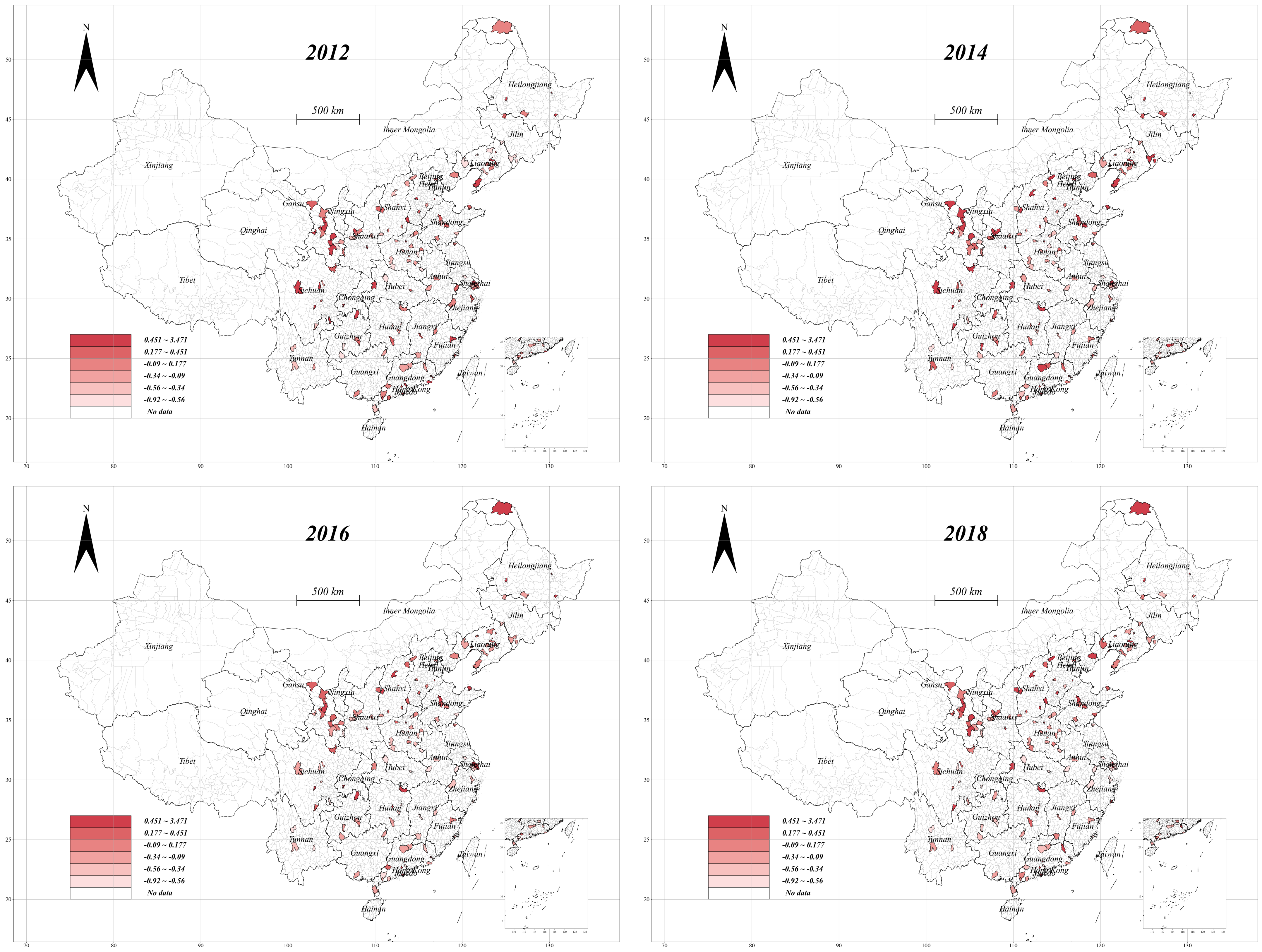
The modified 10% indicator excludes high-income households with high energy use. PCA combines the three components into the composite EPI [19]. Descriptive statistics and PCA weights are reported in

Table A1. Indicators of energy poverty index.

VarName	Min	Max	Mean	SD
Improved 10% indicator	0.000	1.000	0.277	0.447
Cooking cleanliness	0.000	1.000	0.529	0.499
Percentage of energy expenditure	0.000	0.446	0.088	0.111

and

Table A2. Energy poverty index system.

VarName	Variables	Weights
Affordability	Improved 10% indicator	0.4921
	Percentage of energy expenditure	0.3345
Accessibility	Cooking cleanliness	0.1734

Note: The weights are calculated from PCA.

of Appendix A. Following the established specification, both affordability measures are retained because the continuous share records burden intensity, whereas the modified 10% indicator identifies low-income households above the threshold. Section 4.3 separately estimates total energy and electricity expenditure responses, so the interpretation is not based solely on the composite EPI. Figure 1 maps county averages of the resulting EPI.

3.3. Heat Shocks

Previous studies recommended several temperature-shock methods. In this study, temperature deviations were used to detect shocks. The variances were determined as the difference between the actual temperature and historical average within a district in a given year divided by the historical standard deviation for the same district. This method has been frequently used in previous studies [63,65,66]. Historical temperatures were recorded from 1980 to 2009 prior to our evaluation period. Therefore, our primary measure of a heat shock is a dummy variable that equals one if the temperature deviates by more than two standard deviations from the historical average.

We defined our heat shock variable in this way for various reasons. First, we suggest that level changes are important in proportion to the district’s normal volatility rather than in absolute terms. The use of relative values also allows for the deduction of differences owing to different climate types in different regions. Therefore, the temperature bin method was not employed in this study.

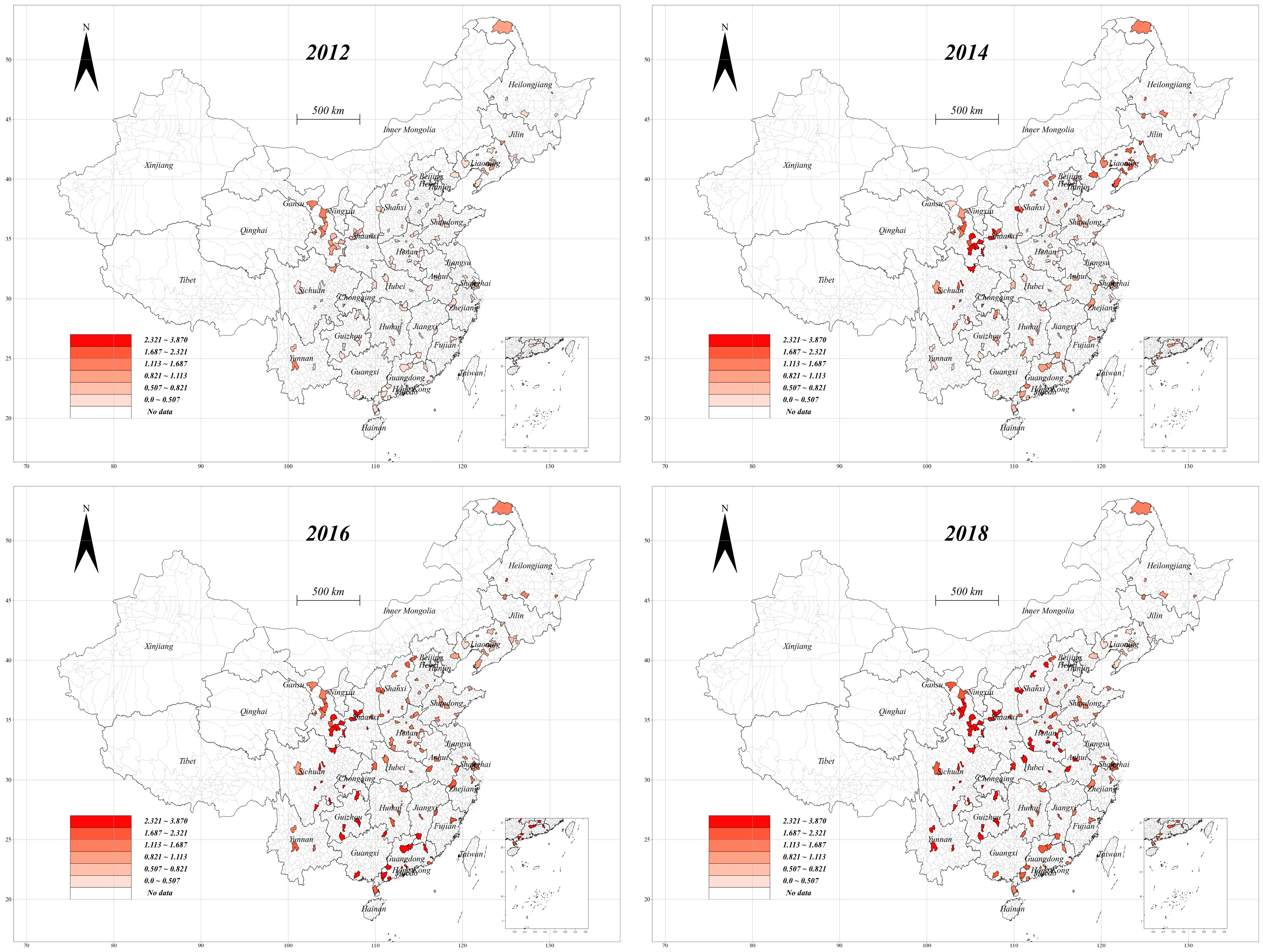
We used wet-bulb temperature because it incorporates both temperature and humidity and therefore represents heat stress more directly than dry-bulb temperature alone. Wet-bulb temperature is the lowest temperature to which air can be cooled through evaporation at constant pressure. Following the cited literature, the main indicator identifies deviations above the historical county distribution, and alternative standard-deviation thresholds are used for sensitivity analysis. Figure 2 shows the spatial distribution of county-level heat shocks.

We also used the annual number of hot days above wet-bulb temperature thresholds as an alternative heat-shock measure [9]. For each county-year, HD22 and HD25 count the days on which average daily wet-bulb temperature exceeds 22 °C and 25 °C, respectively. These counts are also used to construct the dynamic inter-wave cumulative exposure measure [67,68]. The deviation-based indicator is used in the contemporaneous specifications, whereas cumulative hot-day counts are used in the adjacent-wave model.

We selected two thresholds for elevated heat shock: 22 degrees wet bulb and 25 degrees wet bulb. The following served as the basis for the choice: it is considered to be extremely hazardous when the wet-bulb temperature reaches 29.1 degrees. According to theory, the human body’s physiological limit for wet bulb temperature is 35 degrees Celsius, at which point it is incapable of dissipating heat through sweating. According to certain conventional home air-conditioning manuals, the typical range for wet-bulb temperatures in air conditioning is 26 degrees. Certain sources of literature indicate that the human impact is significantly increased when the wet-bulb temperature exceeds 22 degrees. Some individuals will be at risk of health complications if the wet-bulb temperature exceeds 24.6 degrees, as indicated by pertinent research [69,70]. After considering all of the aforementioned, we selected 22 and 25 degrees as the thresholds for wet-bulb temperatures in our analysis.

3.4. Econometric Model

3.4.1. Baseline Model

This study estimates the association between heat shocks and energy poverty. The heat-shock variable is defined as the difference between current county-level wet-bulb temperature and its historical reference distribution. To give the PCA-based outcome a common interpretive scale, we standardized the EPI so that the estimated coefficients can be interpreted in standard-deviation units. The standardized energy poverty index (EPI) was the dependent variable, whereas heat shock (HS) was the key independent variable. Descriptive statistics of the variables involved in the econometric model are shown in

Table A3. Summary statistics of variables in the econometric model.

Var Name	Description	Mean	SD
EPI	Using a composite index constructed by improving the 10% indicator, household energy expenditure as a percentage of income, and the cleanliness of cooking fuels to measure energy poverty	−0.010	0.928
Heat shocks (2 SD)	=1 if the wet-bulb temperature exceeds the historical mean by 2 standard deviations	0.520	0.500
Heat shocks (2.5 SD)	=1 if the wet-bulb temperature exceeds the historical mean by 2.5 standard deviations	0.297	0.457
Heat shocks (3 SD)	=1 if the wet-bulb temperature exceeds the historical mean by 3 standard deviations	0.155	0.362
Numbers of hot days (25 °C)	The number of days in the year when the average daily wet-bulb temperature was above 25 °C	8.448	20.658
Numbers of hot days (22 °C)	The number of days in the year when the average daily wet-bulb temperature was above 22 °C	33.206	46.336
Gender	Gender of the head of household	0.615	0.487
Age	Age of head of household	52.407	13.488
Education	=1 indicates education level beyond secondary school	0.256	0.436
Married	=1 indicates that the head of household is married	0.856	0.352
Household size	Indicates the number of people in the household	4.106	1.934
Home ownership	=1 indicates that the housing is owned by the head of household	0.942	0.234
Employ	=1 means the head of household has a job	0.816	0.388
Family income (Log)	Total income of households in the year of the survey	10.310	1.170
Remote areas	=1 indicates far from the provincial capital city	0.502	0.500
Surface temperature	Average annual surface temperature (°C)	13.317	4.731
Wind speed	Annual average wind speed at 2 m above ground (m/s)	1.815	0.645
Precipitation	Average annual precipitation (kg/m2)	0.049	0.024
Pressure	Annual average sea-level pressure (Pa)	101,431.312	256.879
Humidity	Annual average specific humidity (kg/kg)	0.008	0.003

. According to Feeny et al. (2021) [9], the econometric model is designed as follows:

$${EPI}_{i\mathrm{c},\mathrm{t}}=\alpha +{\beta }_1{HS}_{ct}+{\beta }_2{X}_{ic,t}+{\mu }_p+{\delta }_t+{\mu }_p\times {\lambda }_t+{\epsilon }_{ic,t}$$

(1)

where ${EPI}_{ic,t}$ denotes the energy poverty status of household i in county c in year t (2012–2018). ${HS}_{ct}$ is the key explanatory variable. To measure ${HS}_{ct}$, this study first quantified the disparity between the mean temperature values of the observed variable in county c during year t and the historical mean of the country’s temperature spanning the period from 1980 to 2009, with the resulting value normalized by the historical standard deviation. We ascribed significance to level changes not solely in absolute magnitudes but also in relation to their deviation from the historical mean. If the difference between the observed temperature and the country’s historical mean temperature surpassed a threshold of two standard deviations, heat shocks were considered to have occurred. Furthermore, we employed the number of days in the current year with high wet-bulb temperatures as a metric for heat shocks. The wet-bulb temperature standards of 22 and 25 degrees (HD22; HD25) were still utilized for counting.

$X_{ic,t}$ is a vector comprising a set of control variables. Our study’s control variables consist of household socioeconomic characteristic variables, namely gender of household head, age of household head, education level, marital status, household size, housing ownership, and employment status; regional control variables, consisting of energy price, urbanization level, and GDP per capita; and regional climate variables, namely average annual surface temperature, average annual wind speed, average annual precipitation, and average annual humidity. ${\mu }_p$ is the provincial fixed effect, ${\delta }_t$ is the time fixed effect, and ${\lambda }_t$ is the linear temporal trend. By adding provincial fixed effects, we considered time-invariant elements at the provincial level that influence energy poverty, whereas time fixed effects account for any cross-province time trends in energy poverty. To account for provincial-specific macroeconomic trends, the model also included interactions between provincial effects and linear temporal trends. The random disturbance term with an independent and identical distribution is denoted by ${\epsilon }_{ic,t}$.

After controlling for the geographical and temporal fixed variables, as well as province–linear time interactions, the fundamental premise of Equation (1) is that heat shocks were as random as possible. Obviously, there is no assurance that if a heat shock did not occur, the trends across an impacted province would have followed the same time-series pattern as a non-affected province. The potential bias in the estimation results arises primarily from two factors. First, China has experienced rapid economic growth in recent decades; however, regional disparities exist. Second, the living conditions of rural inhabitants have improved vastly because of the Chinese government’s heightened focus on rural development. We attempted to address these problems in two ways. First, this study considers linear time-province fixed effects. Second, our study covers only the years 2012–2018, which is not a very long period.

3.4.2. Hidden Energy Poverty: Analysis of Energy Spending Gap

Household energy poverty appears as inadequate energy services or an inability to utilize energy at desirable levels in nations where modern energy infrastructure is widely available. Consequently, a more inclusive definition of energy poverty needs to encompass both families that exhibit energy-constrained behavior (limiting their energy spending) and those that have high energy burdens (expenditures relative to energy bills) [32]. Based on pertinent literature, we estimated the differences in energy expenditure between low-income and higher-income households in response to temperature in order to analyze the problem of hidden energy poverty as it is presented in this study.

We investigated whether households with higher and lower incomes react to heat shocks in the same way in terms of energy spending. Next, we estimated a model that takes into account how different households with varying income levels are affected differently by heat shocks when it comes to energy spending. We specifically modeled the interaction between the income grouping variable and the quantity of hot days.

$${ln(EnergySpend}_{ic,t})=\alpha +{\beta }_1{HD}_{ct}+{\beta }_2{HD}_{ct}\times {IG}_{ic,t}+{\beta }_3{IG}_{ic,t}+{\beta }_4{X}_{ic,t}+{\mu }_p+{\delta }_t+{\mu }_p\times {\lambda }_t+{\epsilon }_{ic,t}$$

(2)

where ${EnergySpend}_{ic,t}$ denotes the energy spending of household i in county c in year t (2012–2018). ${HD}_{ct}$ stands for the total number of days with high temperatures in region c during year t. We counted using the wet-bulb temperature standards of 22 and 25 degrees (HD22; HD25). ${IG}_{ic,t}$ is a dummy variable that uses the median income of the rural households in the sample to categorize households into high- and low-income groups. Households above the median are recorded as high-income households and take the value of 1, while households below the median are recorded as low-income households and take the value of 0. We also established two methods for income grouping. The first method involves dividing the sample based on the median of the entire sample (IG_all). Households that exceed the median income of the entire sample are designated as high-income households, while those that fall below the median income are designated as low-income households. The second criterion is determined by the median income of the sample in the household’s local province (IG_region). Households that exceed the median income of the local province are classified as high-income, while those that fall below the median income are classified as low-income. Because the logarithm is undefined at zero, observations reporting zero expenditure are omitted only from the corresponding log specification. There are 232 zero total-energy-expenditure observations and 2464 zero electricity-expenditure observations, leaving 20,952 and 18,720 observations in the corresponding log-model samples, respectively. As a zero-inclusive robustness check, we applied the inverse hyperbolic sine (IHS) transformation. The IHS is defined at zero, retains zero-expenditure observations, and approximates a logarithmic transformation at larger positive values; the corresponding estimates are reported in Appendix A 

Table A5. Zero-inclusive robustness checks using the inverse hyperbolic sine (IHS) transformation.

	(1)	(2)	(3)	(4)
VARIABLES	IHS(Energy Spending)	IHS(Energy Spending)	IHS(Electricity)	IHS(Electricity)
	HD25	HD22	HD25	HD22
Panel A. National income cutoff
HD25	−0.00195 * (0.00112)		−0.00497 *** (0.00181)
High income × HD25	0.00329 *** (0.000797)		0.00390 *** (0.00129)
HD22		0.00663 *** (0.00133)		0.00274 (0.00215)
High income × HD22		0.00161 *** (0.000355)		0.00239 *** (0.000575)
High-income household	0.0123 (0.0244)	−0.0114 (0.0259)	0.0444 (0.0396)	0.00284 (0.0420)
Constant	−57.1 *** (10.1)	−61.6 *** (10.0)	−82.1 *** (16.4)	−89.3 *** (16.3)
Controls	YES	YES	YES	YES
Province × wave FE	YES	YES	YES	YES
Observations	21,184	21,184	21,184	21,184
R-squared	0.173	0.175	0.412	0.412
Panel B. Province-specific income cutoff
HD25	−0.00149 (0.00109)		−0.00467 *** (0.00177)
High income × HD25	0.00280 *** (0.000780)		0.00378 *** (0.00126)
HD22		0.00666 *** (0.00133)		0.00258 (0.00215)
High income × HD22		0.00163 *** (0.000348)		0.00280 *** (0.000564)
High-income household	0.0223 (0.0244)	−0.00543 (0.0260)	0.0505 (0.0396)	−0.00626 (0.0421)
Constant	−57.2 *** (10.1)	−61.2 *** (10.0)	−82.3 *** (16.4)	−88.9 *** (16.3)
Controls	YES	YES	YES	YES
Province × wave FE	YES	YES	YES	YES
Observations	21,184	21,184	21,184	21,184
R-squared	0.173	0.175	0.412	0.412

Notes: The dependent variables are inverse-hyperbolic-sine transformations of total energy and electricity expenditures, so zero values are retained. Coefficients and standard errors are reported to three significant figures, with standard errors in parentheses; significance is calculated from the unrounded estimates. All models use the original controls and province-by-wave fixed effects. The stars refer to two-sided tests where the corresponding coefficient equals zero: *** p < 0.01, ** p < 0.05, * p < 0.1.

.

The remaining components of the model, including the control variables mentioned earlier, are the same as those in Equation (1) and will not be discussed again. Should it be determined that there are variations in energy spending in reaction to high temperatures among various income brackets, this indicates that low-income households might exhibit energy-saving behaviors, thereby exhibiting hidden energy poverty. Policymakers must focus their aid on helping these vulnerable rural households adjust to extreme heat by using the findings of these analyses.

3.4.3. Inter-Wave Cumulative-Exposure Model

The preceding models examined contemporaneous responses within each survey wave. Equation (3) extends the analysis by relating changes in household energy poverty across adjacent CFPS waves to cumulative hot-day exposure. The specification captures the net dynamic inter-wave association after household production, employment, and energy-use adjustments; it does not separately identify individual adaptation mechanisms [67,68].

$${EPI}_{ic,t}-{EPI}_{ic,t-1}=\alpha +{\beta }_{LD}{\int }_{t-1}^t{HD}_{ic,t}dt+{\gamma }_1(X_{ic,t}-X_{ic,t-1})+{\mu }_p+{\epsilon }_{it}$$

(3)

where i represents the household, c represents the county, and t represents the year. ${\int }_{t-1}^t{HD}_{ic,t}dt$ denotes cumulative hot-day exposure for the adjacent-wave comparison. We retained the 22 °C and 25 °C wet-bulb thresholds. ${\int }_{t-1}^t{HD}_{ic,t}dt$ is the sum of annual hot-day counts over the inclusive exposure window. X is a control variable, as described above. Provincial fixed effects (${\mu }_p$) account for time-invariant elements at the provincial level that influence energy poverty. The random disturbance term with an independent and identical distribution is denoted by ${\epsilon }_{it}$. The parameter ${\beta }_{LD}$ captures the association between cumulative hot-day exposure and the inter-wave change in the standardized EPI. As standardization does not affect the first-difference interpretation, the estimated changes are expressed in standard-deviation units, consistent with the other EPI analyses. For an adjacent-wave comparison, the exposure sum includes the starting survey year, the intervening year, and the ending survey year. Thus, the 2016–2018 comparison includes 2016, 2017, and 2018: a three-calendar-year inclusive exposure window even though the two interviews are two years apart.

4. Empirical Results

The results are presented in four parts. Section 4.1 reports the baseline estimates, Section 4.2 and Section 4.3 examine regional and income-related heterogeneity, and Section 4.4 presents the dynamic inter-wave cumulative analysis. For brevity, the tables report the core coefficients.

4.1. Main Results

Table 1. Impacts of heat shocks on energy poverty.

	(1)	(2)	(3)	(4)	(5)
Variables	EPI (SD Units)	EPI (SD Units)	EPI (SD Units)	EPI (SD Units)	EPI (SD Units)
Heat shocks (2 SD)	0.164 ***
	(0.0198)
Heat shocks (2.5 SD)		0.163 ***
		(0.0166)
Heat shocks (3 SD)			0.0503 **
			(0.0201)
HD25				0.00364 ***
				(0.000640)
HD22					0.00287 ***
					(0.000830)
Constant	1.44	7.66	−3.32	−10.2	−12.3
	(20.5)	(20.5)	(20.5)	(20.6)	(20.8)
Controls	YES	YES	YES	YES	YES
Province FE	YES	YES	YES	YES	YES
Year FE	YES	YES	YES	YES	YES
Province * linear time	YES	YES	YES	YES	YES
Observations	21,184	21,184	21,184	21,184	21,184
R-squared	0.468	0.469	0.467	0.468	0.467

The dependent variable is standardized as EPI_z = [EPI − mean(EPI)]/SD(EPI), where mean(EPI) = −0.010456 and SD(EPI) = 0.927999. Coefficients and standard errors are reported to three significant figures, with standard errors in parentheses. Significance levels are calculated from the unrounded estimates. The stars refer to two-sided p-values for tests where the corresponding coefficient equals zero: *** p < 0.01, ** p < 0.05, * p < 0.1.

reports the estimates from Equation (1) using the standardized EPI defined in Section 3.4.1. Subtracting the sample mean changes only the intercept, while dividing the dependent variable and its standard error by SD(EPI) = 0.927999 expresses the slope estimates in standard-deviation units; the t statistics, p-values, and significance levels are unchanged. Columns (1)–(3) show positive and statistically significant coefficients of 0.164, 0.163, and 0.0503 under the 2-, 2.5-, and 3-SD definitions, respectively. The HD25 and HD22 coefficients are 0.00364 and 0.00287 EPI standard deviations per additional hot day. The smaller 3-SD coefficient does not by itself establish a discontinuity because the indicators are nested and each separate regression changes both the exposed group and its comparison group. The exposed share also declines from 52.0% at 2 SD to 29.7% at 2.5 SD and 15.5% at 3 SD. The results therefore support the same positive conclusion across the submitted definitions but should not be read as a monotonic dose–response test.

The two heat-shock measures capture complementary dimensions of exposure. The standard-deviation indicators measure wet-bulb temperature relative to the county’s historical distribution, whereas HD22 and HD25 measure the annual frequency of days above absolute wet-bulb thresholds. Both approaches yield positive coefficients in Table 1. Possible pathways include cooling-related expenditure, labor productivity, and agricultural income. Although China has now eradicated absolute poverty [71,72,73], rural infrastructure remains deficient, and climate change exacerbates energy poverty, which may jeopardize its progress in the fight against poverty. The present models do not separately identify the possible mechanisms.

4.2. Impact of Heat Shocks on Energy Poverty: Regional Heterogeneity Analysis

China is a vast country, with significant differences between its northern and southern regions. These differences are primarily reflected in climatic, agricultural production, and rural lifestyle differences. Further analysis of the heterogeneity in China’s northern and southern regions can aid in gaining a better understanding of the impact of heat shocks on energy poverty. The groupings in the North and South are listed in

Table A4. The specific provinces across different regions.

Region	Provinces
North (15 provinces)	Beijing, Hebei, Tianjin, Inner Mongolia, Shanxi, Jilin, Liaoning, Heilongjiang, Henan, Shandong, Gansu, Shaanxi, Ningxia, Qinghai, Xinjiang
South (15 provinces)	Shanghai, Jiangsu, Hainan, Fujian, Hubei, Jiangxi, Guangxi, Hunan, Guangdong, Sichuan, Guizhou, Chongqing, Zhejiang, Anhui, Yunnan

.

Table 2. Regional heterogeneity analysis (1).

	(1)	(2)
	North	South
Variables	EPI (SD Units)	EPI (SD Units)
Heat shocks (2 SD)	0.177 ***	−0.00785
	(0.0240)	(0.0427)
R-squared	0.465	0.471
Heat shocks (2.5 SD)	0.215 ***	0.0251
	(0.0211)	(0.0356)
R-squared	0.467	0.471
Heat shocks (3 SD)	−0.0159	0.0976 ***
	(0.0266)	(0.0366)
Controls	YES	YES
Province FE	YES	YES
Year FE	YES	YES
Province * linear time	YES	YES
R-squared	0.463	0.471
Observations	13,162	8022

The dependent variable is standardized as EPI_z = [EPI − mean(EPI)]/SD(EPI), where mean(EPI) = −0.010456 and SD(EPI) = 0.927999. Coefficients and standard errors are reported to three significant figures, with standard errors in parentheses. Significance levels are calculated from the unrounded estimates. The stars refer to two-sided p-values for tests where the corresponding coefficient equals zero: *** p < 0.01, ** p < 0.05, * p < 0.1.

reports the North–South heterogeneity estimates. In northern China, the coefficients are positive and statistically significant under the 2- and 2.5-SD definitions, whereas the 3-SD coefficient is not statistically significant. In southern China, a positive and statistically significant coefficient appears under the 3-SD definition. Because event frequency and comparison-group composition differ across thresholds and regions, these estimates are interpreted as heterogeneous patterns rather than as a formal monotonic comparison of heat sensitivity.

Aside from the North–South divide in China, the intra-provincial distribution of rural areas may also introduce variations in the impact of heat shocks on energy poverty. Rural areas close to cities are also more likely to be more developed. For example, rural areas adjacent to cities benefit from urban development dividends as the cities expand. Science and technology can provide more support to rural areas near cities. Urban residents will have more demand for leisure and vacations, and rural residents will find it more convenient to engage in non-agricultural employment. Therefore, rural areas near cities are more likely to be economically developed and resilient to heat shocks, resulting in lower levels of energy poverty. Due to the concentration of the majority of a province’s economic and technological resources in provincial capital cities, which serve as the core cities in provincial economic circles, we employed the proximity of rural areas to provincial capital cities as a proxy variable to determine whether rural areas are adjacent to urban centers. The average distance between the sample county and provincial capital was used as the threshold in this study, and values greater than this were classified as being far away from the provincial capital, that is, remote rural areas.

Table 3. Regional heterogeneity analysis (2).

	(1)	(2)
	Close to the Provincial Capital	Away from the Provincial Capital
Variables	EPI (SD Units)	EPI (SD Units)
Heat shocks (2 SD)	0.108 ***	0.197 ***
	(0.0315)	(0.0460)
R-squared	0.476	0.467
Heat shocks (2.5 SD)	−0.0441	0.202 ***
	(0.0318)	(0.0279)
R-squared	0.475	0.469
Heat shocks (3 SD)	−0.0424	0.0937 ***
	(0.0705)	(0.0359)
Controls	YES	YES
R-squared	0.475	0.467
Province FE	YES	YES
Year FE	YES	YES
Province * linear time	YES	YES
Observations	10,551	10,633

The dependent variable is standardized as EPI_z = [EPI − mean(EPI)]/SD(EPI), where mean(EPI) = −0.010456 and SD(EPI) = 0.927999. Coefficients and standard errors are reported to three significant figures, with standard errors in parentheses. Significance levels are calculated from the unrounded estimates. The stars refer to two-sided p-values for tests where the corresponding coefficient equals zero: *** p < 0.01, ** p < 0.05, * p < 0.1.

shows the heterogeneity analysis of whether the county is far from the provincial capital city. Under the heat shocks with a two-standard-deviation threshold, both remote areas and adjacent provincial capitals showed a statistically significant increase in the degree of energy poverty. However, the impact was greater in remote rural areas. Only remote rural areas showed an increase in energy poverty under more intense heat shocks (2.5 SD; 3 SD).

4.3. Results of Hidden Energy Poverty Analysis

Energy expenditure is commonly used to identify energy poverty because it directly reflects the affordability of household energy use. However, expenditure-based indicators may not fully capture households that restrict energy use because of financial constraints. This issue is particularly relevant under heat shocks. Higher temperatures increase the need for cooling, but low-income households may be unable to increase energy use sufficiently and may instead endure heat exposure to prioritize other basic expenditures, such as food, healthcare, or education. In this case, relatively low energy spending does not necessarily indicate adequate energy services. It may instead reflect constrained energy use. To examine this issue, this section compares the energy expenditure responses of low- and higher-income rural households to hot days.

Table 4. Analysis of energy spending gap: grouping is based on the income of the full sample.

	(1)	(2)	(3)	(4)
Variables	ln(Energy Spending)	ln(Energy Spending)	ln(Electricity)	ln(Electricity)
HD25	0.00170 **		0.000285
	(0.000830)		(0.000709)
IG_all × HD25	0.00120 **		0.00211 ***
	(0.000595)		(0.000501)
HD22		0.00940 ***		0.00453 ***
		(0.000983)		(0.000831)
IG_all × HD22		0.000736 ***		0.000798 ***
		(0.000263)		(0.000226)
IG_all	0.0654 ***	0.0518 ***	0.0629 ***	0.0548 ***
	(0.0181)	(0.0192)	(0.0158)	(0.0167)
Constant	−34.7 ***	−36.0 ***	−1.36	−1.78
	(7.53)	(7.44)	(6.73)	(6.66)
Controls	YES	YES	YES	YES
Province FE	YES	YES	YES	YES
Year FE	YES	YES	YES	YES
Province * linear time	YES	YES	YES	YES
R-squared	0.216	0.220	0.276	0.277

Coefficients and standard errors are reported to three significant figures, with leading zeros retained as needed; standard errors are reported in parentheses. Significance levels are calculated from the unrounded estimates. The stars refer to two-sided p-values for tests where the corresponding coefficient equals zero: *** p < 0.01, ** p < 0.05, * p < 0.1.

reports the results of the energy spending gap analysis when households are grouped according to the median income of the full sample. Columns (1) and (2) use total household energy spending as the dependent variable, while Columns (3) and (4) use household electricity spending. In Columns (1) and (2), both the hot-day variables and their interaction terms with the income-group dummy are positive and statistically significant. This indicates that energy spending increases with the number of hot days, but the increase is larger for higher-income households than for lower-income households. Specifically, when the wet-bulb temperature exceeds 25 °C, an additional hot day is associated with a 0.17% increase in energy spending for low-income households and a 0.29% increase for higher-income households. When the wet-bulb temperature exceeds 22 °C, an additional hot day is associated with a 0.94% increase in energy spending for low-income households and a 1.01% increase for higher-income households.

The results for electricity spending show a similar pattern, although the estimate in Column (3) should be interpreted with caution because the coefficient of HD25 is not statistically significant. Nevertheless, the positive and significant interaction term in Column (3) suggests that higher-income households show a stronger electricity spending response to hot days above 25 °C. In Column (4), both HD22 and its interaction with the income-group dummy are statistically significant. An additional day with wet-bulb temperature above 22 °C is associated with a 0.453% increase in electricity spending for low-income households and a 0.533% increase for higher-income households. Overall, the results in Table 4 suggest that low-income rural households increase their energy and electricity spending less than higher-income households under heat shocks. This pattern is consistent with the possibility that affordability constraints limit the ability of low-income households to increase energy use in response to extreme heat.

Table 5. Analysis of energy spending gap: grouping is based on income within each province.

	(1)	(2)	(3)	(4)
Variables	ln(Energy Spending)	ln(Energy Spending)	ln(Electricity)	ln(Electricity)
HD25	0.00213 ***		0.000548
	(0.000812)		(0.000692)
IG_region × HD25	0.000483		0.00184 ***
	(0.000581)		(0.000489)
HD22		0.00951 ***		0.00453 ***
		(0.000982)		(0.000830)
IG_region × HD22		0.000587 **		0.000876 ***
		(0.000259)		(0.000221)
IG_region	0.0634 ***	0.0499 ***	0.0531 ***	0.0413 **
	(0.0181)	(0.0192)	(0.0158)	(0.0168)
Constant	−34.9 ***	−36.0 ***	−1.59	−1.74
	(7.53)	(7.44)	(6.73)	(6.66)
Controls	YES	YES	YES	YES
Province FE	YES	YES	YES	YES
Year FE	YES	YES	YES	YES
Province * linear time	YES	YES	YES	YES
R-squared	0.220	0.224	0.276	0.277

Coefficients and standard errors are reported to three significant figures, with leading zeros retained as needed; standard errors are reported in parentheses. Significance levels are calculated from the unrounded estimates. The stars refer to two-sided p-values for tests where the corresponding coefficient equals zero: *** p < 0.01, ** p < 0.05, * p < 0.1.

reports the results when households are grouped according to the median income within each province. The signs of the key variables are generally consistent with those in Table 4, indicating that the results are not driven by a particular income-grouping method. In Column (1), HD25 is positive and statistically significant, showing that an additional day with wet-bulb temperature above 25 °C increases energy spending by 0.213% for low-income households. However, the interaction term between HD25 and the regional income-group dummy is not statistically significant, so this column does not provide strong evidence of a significant difference between low- and higher-income households under the 25 °C threshold.

In Column (2), both HD22 and its interaction term are statistically significant. An additional day with wet-bulb temperature above 22 °C increases energy spending by 0.951% for low-income households and by 1.010% for higher-income households. For electricity spending, the coefficient of HD25 in Column (3) is not statistically significant, so the baseline electricity response under the 25 °C threshold should be interpreted with caution. Nevertheless, the interaction term in Column (3) is positive and statistically significant, suggesting that higher-income households exhibit a stronger electricity spending response to hot days above 25 °C. In Column (4), both HD22 and its interaction term are statistically significant. An additional day with wet-bulb temperature above 22 °C increases electricity spending by 0.453% for low-income households and by 0.541% for higher-income households.

Taken together, Table 4 and Table 5 show that rural households with different income levels respond differently to heat shocks in terms of energy and electricity spending. Higher-income households generally increase their spending more strongly, while low-income households show a weaker spending response. Following the logic of this study, this weaker response does not mean that low-income households have lower cooling needs under heat shocks. Rather, it indicates that they are less able to increase energy use because of affordability constraints. Therefore, the results provide evidence consistent with hidden energy poverty among low-income rural households under heat shocks. Conventional expenditure-based indicators may underestimate their actual energy deprivation because these households may reduce or suppress necessary energy consumption to relieve financial pressure. The zero-inclusive IHS estimates in Appendix A Table A5 provide the same qualitative evidence for the income-differential pattern: all eight hot-day-by-high-income interaction coefficients are positive and statistically significant at the 1% level.

4.4. Cumulative Effects of Heat Exposure

The preceding analysis focuses on contemporaneous responses within survey waves. The dynamic inter-wave cumulative analysis examines whether the accumulated number of hot days in the inclusive exposure window is associated with changes in household energy poverty between adjacent CFPS interviews. This specification summarizes the net inter-wave relationship after any household adjustments; it does not separately estimate a specific adaptation mechanism.

Table 6. Dynamic inter-wave cumulative association between heat shocks and energy poverty.

	(1)	(2)
Variables	D.EPI (SD Units)	D.EPI (SD Units)
The total number of hot days (25 °C)	0.00310 **
	(0.00125)
The total number of hot days (22 °C)		0.00298 **
		(0.00137)
Constant	187 **	166 **
	(79.4)	(80.5)
Controls	YES	YES
Province FE	YES	YES
Year FE	YES	YES
Observations	5822	5822
R-squared	0.175	0.175

The dependent variable is standardized as EPI_z = [EPI − mean(EPI)]/SD(EPI), where mean(EPI) = −0.010456 and SD(EPI) = 0.927999. Coefficients and standard errors are reported to three significant figures, with standard errors in parentheses. Significance levels are calculated from the unrounded estimates. The stars refer to two-sided p-values for tests where the corresponding coefficient equals zero: *** p < 0.01, ** p < 0.05, * p < 0.1.

reports the dynamic inter-wave cumulative estimates from Equation (3) using the change in the standardized EPI. The coefficients on cumulative HD25 and HD22 are 0.00310 and 0.00298, respectively, and remain statistically significant at the 5% level. Thus, greater cumulative hot-day exposure is associated with an increase in the standardized EPI between adjacent survey waves. This pattern is consistent with persistent vulnerability, and it should be interpreted as a dynamic inter-wave association rather than as a separately identified adaptation effect.

4.5. Discussion and Limitations

The original specifications consistently indicate a positive relationship between heat shocks and rural energy poverty, while the weaker spending response among low-income households is consistent with hidden energy poverty. The EPI follows Lin and Zhao (2021) [19], and the expenditure analysis provides complementary evidence beyond the composite index. These expenditure differences are consistent with constrained energy use, but they do not directly measure unmet cooling needs, indoor comfort, or appliance operation.

Future research could use longer household panels and direct measures of indoor temperature, cooling-appliance operation, energy quantities, unmet cooling needs, and indoor comfort. Richer information on irrigation demand, agricultural production and income, health, labor supply, and household adaptation could also distinguish the mechanisms linking heat exposure to energy poverty; these mechanisms are not directly tested in the present study.

5. Conclusions and Policy Implications

This study examines the impact of heat shocks on energy poverty among rural households in China. Using household-level data from the China Family Panel Studies and NASA climate data, we construct a household energy poverty index and measure heat shocks based on wet-bulb temperature. The main findings are as follows.

First, heat shocks significantly increase rural household energy poverty. This result remains robust when alternative indicators of heat shocks are used, including different standard-deviation thresholds and numbers of hot days above wet-bulb temperature thresholds. These findings indicate that extreme heat is not only a climate and health risk, but also an important factor shaping household energy affordability and energy poverty.

Second, the impact of heat shocks is heterogeneous across regions. Rural households in northern China are more sensitive to heat shocks than those in southern China, especially under moderate heat shock thresholds. Rural households located farther from provincial capitals are also more vulnerable. These findings suggest that the effect of heat shocks is closely related to local climate conditions, infrastructure, economic opportunities, and access to adaptive resources.

Third, the results provide evidence consistent with hidden energy poverty among low-income rural households under heat shocks. Compared with higher-income households, low-income households show a weaker increase in energy and electricity spending when hot days increase. When wet-bulb temperature exceeds 25 °C, low-income households increase energy spending by 0.17% per additional hot day, while higher-income households increase energy spending by 0.29%. When wet-bulb temperature exceeds 22 °C, the corresponding increases are 0.94% and 1.01%, respectively. For electricity spending, each additional day above 22 °C increases expenditure by 0.453% for low-income households and 0.541% for higher-income households. Following the logic of this study, the weaker expenditure response of low-income households does not imply lower cooling needs. Rather, it suggests that affordability constraints may prevent them from increasing energy use sufficiently under extreme heat. Conventional expenditure-based indicators may therefore underestimate their actual energy deprivation.

Fourth, the dynamic inter-wave cumulative estimates are positive and statistically significant under both hot-day thresholds in the submitted specification. This indicates that the association between heat exposure and energy poverty extends across adjacent survey waves. Although households may adjust production, employment, or energy-use behavior, the model captures only the net inter-wave relationship and does not separately identify those adjustments.

These findings have several policy implications. First, energy poverty policy should pay greater attention to climate-related cooling needs. In the context of global warming, rural energy poverty is not only a winter heating or clean-cooking issue. Extreme heat increases the need for cooling, ventilation, and stable electricity supply. Public policies should incorporate heat-related energy needs into energy poverty identification, rural welfare policy, and climate adaptation planning.

Second, rural infrastructure should be strengthened to improve households’ adaptive capacity. This includes improving housing insulation and ventilation, ensuring stable electricity supply in remote areas, and strengthening local energy system resilience under high-temperature conditions. Accurate heat warnings and climate information should also be delivered to rural households in a practical way, so that households can better prepare for extreme heat events.

Third, regional differences should be considered in policy design. The stronger reported associations in northern China and in areas farther from provincial capitals suggest that a uniform response may overlook differences in climate exposure, infrastructure, economic opportunities, and adaptive resources. Regional targeting should therefore account for local vulnerability and service accessibility.

Fourth, policy support should be more targeted toward remote rural areas. Households far from provincial capitals may have weaker infrastructure, fewer non-agricultural employment opportunities, and more limited access to public services. Rather than relying on uniform policy instruments, energy poverty alleviation should consider local accessibility, infrastructure conditions, and the availability of adaptive resources. Investments in rural electricity reliability, public services, employment training, and local adaptation capacity are particularly important for these areas.

Fifth, low-income households require more precise support under extreme heat. The evidence of hidden energy poverty suggests that some households may reduce necessary energy use to relieve financial pressure. Therefore, energy assistance should not be based only on whether households report high energy expenditure. Policymakers should also identify households that maintain low energy spending because they cannot afford adequate cooling. Targeted summer electricity subsidies, cooling-related assistance, and health support for low-income households can help reduce the risks associated with constrained energy use.

Finally, because the dynamic inter-wave estimates indicate persistent vulnerability, policy intervention should combine short-term emergency responses with sustained adaptation. Improving housing quality, strengthening rural energy infrastructure, supporting livelihood diversification, and enhancing household adaptation capacity can help prevent repeated heat exposure from becoming sustained energy vulnerability. These measures are important for consolidating poverty-reduction achievements and building a more climate-resilient rural energy system.

References

1. Xing, Q.; Sun, Z.; Tao, Y.; Shang, J.; Miao, S.; Xiao, C.; Zheng, C. Projections of future temperature-related cardiovascular mortality under climate change, urbanization and population aging in Beijing, China. Environ. Int. 2022, 163, 107231. [Google Scholar] [CrossRef] [Scilit]
2. Zhou, L.; He, C.; Kim, H.; Honda, Y.; Lee, W.; Hashizume, M.; Chen, R.; Kan, H. The burden of heat-related stroke mortality under climate change scenarios in 22 East Asian cities. Environ. Int. 2022, 170, 107602. [Google Scholar] [CrossRef] [Scilit]
3. Cole, R.; Hajat, S.; Murage, P.; Heaviside, C.; Macintyre, H.; Davies, M.; Wilkinson, P. The contribution of demographic changes to future heat-related health burdens under climate change scenarios. Environ. Int. 2023, 173, 107836. [Google Scholar] [CrossRef] [Scilit]
4. Jurgilevich, A.; Käyhkö, J.; Räsänen, A.; Pörsti, S.; Lagström, H.; Käyhkö, J.; Juhola, S. Factors influencing vulnerability to climate change-related health impacts in cities—A conceptual framework. Environ. Int. 2023, 173, 107837. [Google Scholar] [CrossRef] [Scilit]
5. Carleton, T.A. Crop-damaging temperatures increase suicide rates in India. Proc. Natl. Acad. Sci. USA 2017, 114, 8746–8751. [Google Scholar] [CrossRef] [Scilit]
6. Skoufias, E.; Rabassa, M.; Olivieri, S. The Poverty Impacts of Climate Change: A Review of the Evidence; The World Bank: Washington, DC, USA, 2011. [Google Scholar] [CrossRef] [Scilit]
7. Chen, S.; Gong, B. Response and adaptation of agriculture to climate change: Evidence from China. J. Dev. Econ. 2021, 148, 102557. [Google Scholar] [CrossRef] [Scilit]
8. Li, X. Hydropower in the Mekong River Basin: A Balancing Test. Environ. Claims J. 2012, 24, 51–69. [Google Scholar] [CrossRef] [Scilit]
9. Feeny, S.; Trinh, T.-A.; Zhu, A. Temperature shocks and energy poverty: Findings from Vietnam. Energy Econ. 2021, 99, 105310. [Google Scholar] [CrossRef] [Scilit]
10. Awaworyi Churchill, S.; Smyth, R.; Trinh, T.-A. Energy poverty, temperature and climate change. Energy Econ. 2022, 114, 106306. [Google Scholar] [CrossRef] [Scilit]
11. United Nations. The Sustainable Development Goals Report 2024; United Nations: New York, NY, USA, 2024. [Google Scholar]
12. Chakravarty, S.; Tavoni, M. Energy poverty alleviation and climate change mitigation: Is there a trade off? Energy Econ. 2013, 40, S67–S73. [Google Scholar] [CrossRef] [Scilit]
13. Ürge-Vorsatz, D.; Tirado Herrero, S. Building synergies between climate change mitigation and energy poverty alleviation. Energy Policy 2012, 49, 83–90. [Google Scholar] [CrossRef] [Scilit]
14. Zhao, J.; Jiang, Q.; Dong, X.; Dong, K. Assessing energy poverty and its effect on CO2 emissions: The case of China. Energy Econ. 2021, 97, 105191. [Google Scholar] [CrossRef] [Scilit]
15. Nguyen, C.P.; Nasir, M.A. An inquiry into the nexus between energy poverty and income inequality in the light of global evidence. Energy Econ. 2021, 99, 105289. [Google Scholar] [CrossRef] [Scilit]
16. Avom, D.; Bangaké, C.; Kamguia, B. Does capital flight set Africa as the seat of darkness? Linking capital flight and energy poverty. Energy 2024, 308, 133033. [Google Scholar] [CrossRef] [Scilit]
17. Xie, X.; Barut, A.; Mohammed, K.S.; Torusdağ, M. Empowering energy access: Exploring financial inclusion’s impact on energy poverty in the fragile five economies. Energy 2024, 309, 133184. [Google Scholar] [CrossRef] [Scilit]
18. Yang, Y.; Jiang, M.; Li, X.; Chen, Y. Energy poverty and household development resilience: Household level evidence from China. Energy 2024, 309, 133003. [Google Scholar] [CrossRef] [Scilit]
19. Lin, B.; Zhao, H. Does off-farm work reduce energy poverty? Evidence from rural China. Sustain. Prod. Consum. 2021, 27, 1822–1829. [Google Scholar] [CrossRef] [Scilit]
20. Saenz, J.L.; Adar, S.D.; Zhang, Y.S.; Wilkens, J.; Chattopadhyay, A.; Lee, J.; Wong, R. Household use of polluting cooking fuels and late-life cognitive function: A harmonized analysis of India, Mexico, and China. Environ. Int. 2021, 156, 106722. [Google Scholar] [CrossRef] [Scilit]
21. Görbig, G.M.; Flacke, J.; Sliuzas, R.; Reckien, D. Unveiling energy poverty risk: A multidimensional analysis of the heat-or-eat dilemma. Energy Res. Soc. Sci. 2025, 125, 104076. [Google Scholar] [CrossRef] [Scilit]
22. Ruiz-Ciarreta, I.; Fernández-Aragón, I.; Ochoa De Aspuru-Gulin, O. Unseen and unreported: Hidden and imputed energy poverty in the Basque Country. Energy Res. Soc. Sci. 2026, 136, 104738. [Google Scholar] [CrossRef] [Scilit]
23. Zhao, Y.; Akter, S.; Golley, J. Energy poverty and unpaid work: Evidence from rural China. Energy Res. Soc. Sci. 2026, 133, 104596. [Google Scholar] [CrossRef] [Scilit]
24. Cheng, Z.; Tani, M.; Wang, H. Energy poverty and entrepreneurship. Energy Econ. 2021, 102, 105469. [Google Scholar] [CrossRef] [Scilit]
25. Qin, J.; Li, W.; Zhang, J. How can energy poverty affect farmers’ health? Evidence from mountainous areas in China. Energy 2024, 290, 130074. [Google Scholar] [CrossRef] [Scilit]
26. Shi, H.; Gao, W.; Xu, H.; Chang, M. Understanding the mechanism of energy poverty affecting irrigation efficiency: Evidence from rural China. Environ. Sci. Pollut. Res. 2022, 29, 70963–70975. [Google Scholar] [CrossRef] [Scilit]
27. Boardman, B. Fuel Poverty: From Cold Homes to Affordable Warmth; Belhaven Press: London, UK, 1991. [Google Scholar]
28. Kahouli, S. An economic approach to the study of the relationship between housing hazards and health: The case of residential fuel poverty in France. Energy Econ. 2020, 85, 104592. [Google Scholar] [CrossRef] [Scilit]
29. Cong, S.; Nock, D.; Qiu, Y.L.; Xing, B. Unveiling hidden energy poverty using the energy equity gap. Nat. Commun. 2022, 13, 2456. [Google Scholar] [CrossRef] [Scilit]
30. Doremus, J.M.; Jacqz, I.; Johnston, S. Sweating the energy bill: Extreme weather, poor households, and the energy spending gap. J. Environ. Econ. Manag. 2022, 112, 102609. [Google Scholar] [CrossRef] [Scilit]
31. Campagnolo, L.; De Cian, E. Distributional consequences of climate change impacts on residential energy demand across Italian households. Energy Econ. 2022, 110, 106020. [Google Scholar] [CrossRef] [Scilit]
32. Falchetta, G.; Mistry, M.N. The role of residential air circulation and cooling demand for electrification planning: Implications of climate change in sub-Saharan Africa. Energy Econ. 2021, 99, 105307. [Google Scholar] [CrossRef] [Scilit]
33. Randazzo, T.; De Cian, E.; Mistry, M.N. Air conditioning and electricity expenditure: The role of climate in temperate countries. Econ. Model. 2020, 90, 273–287. [Google Scholar] [CrossRef] [Scilit]
34. Sanchez-Guevara, C.; Núñez Peiró, M.; Taylor, J.; Mavrogianni, A.; González, J.N. Assessing population vulnerability towards summer energy poverty: Case studies of Madrid and London. Energy Build. 2019, 190, 132–143. [Google Scholar] [CrossRef] [Scilit]
35. Bienvenido-Huertas, D.; Sánchez-García, D.; Rubio-Bellido, C. Analysing natural ventilation to reduce the cooling energy consumption and the fuel poverty of social dwellings in coastal zones. Appl. Energy 2020, 279, 115845. [Google Scholar] [CrossRef] [Scilit]
36. Mashhoodi, B. Land surface temperature and energy expenditures of households in the Netherlands: Winners and losers. Urban Clim. 2020, 34, 100678. [Google Scholar] [CrossRef] [Scilit]
37. Igawa, M.; Piao, X.; Managi, S. The impact of cooling energy needs on subjective well-being: Evidence from Japan. Ecol. Econ. 2022, 198, 107464. [Google Scholar] [CrossRef] [Scilit]
38. Bienvenido-Huertas, D.; Sánchez-García, D.; Rubio-Bellido, C.; Marín-García, D. Potential of applying adaptive strategies in buildings to reduce the severity of fuel poverty according to the climate zone and climate change: The case of Andalusia. Sustain. Cities Soc. 2021, 73, 103088. [Google Scholar] [CrossRef] [Scilit]
39. Eichsteller, M.; Njagi, T.; Nyukuri, E. The role of agriculture in poverty escapes in Kenya—Developing a capabilities approach in the context of climate change. World Dev. 2022, 149, 105705. [Google Scholar] [CrossRef] [Scilit]
40. Maganga, A.M.; Chiwaula, L.; Kambewa, P. Climate induced vulnerability to poverty among smallholder farmers: Evidence from Malawi. World Dev. Perspect. 2021, 21, 100273. [Google Scholar] [CrossRef] [Scilit]
41. Que, N.D.; Van Song, N.; Thuan, T.D.; Van Tien, D.; Van Ha, T.; Phuong, N.T.M.; Huong, N.T.X.; Phuong, P.T.L. How temperature shocks impact energy poverty in Vietnam: Mediating role of financial development and environmental consideration. Environ. Sci. Pollut. Res. 2022, 29, 56114–56127. [Google Scholar] [CrossRef] [Scilit]
42. Li, X.; Chow, K.H.; Zhu, Y.; Lin, Y. Evaluating the impacts of high-temperature outdoor working environments on construction labor productivity in China: A case study of rebar workers. Build. Environ. 2016, 95, 42–52. [Google Scholar] [CrossRef] [Scilit]
43. Yi, W.; Chan, A.P.C. Effects of Heat Stress on Construction Labor Productivity in Hong Kong: A Case Study of Rebar Workers. Int. J. Environ. Res. Public Health 2017, 14, 1055. [Google Scholar] [CrossRef] [Scilit]
44. Kjellstrom, T.; Maître, N.; Saget, C. Working on a Warming Planet: The Impact of Heat Stress on Labour Productivity and Decent Work; International Labour Organization: Geneva, Switzerland, 2019. [Google Scholar]
45. Liu, Z.; Wu, D.; He, B.-J.; Liu, Y.; Zhang, X.; Yu, H.; Jin, G. Using solar house to alleviate energy poverty of rural Qinghai-Tibet region, China: A case study of a novel hybrid heating system. Energy Build. 2018, 178, 294–303. [Google Scholar] [CrossRef] [Scilit]
46. Tang, C.F.; Tan, B.W.; Ozturk, I. Energy consumption and economic growth in Vietnam. Renew. Sustain. Energy Rev. 2016, 54, 1506–1514. [Google Scholar] [CrossRef] [Scilit]
47. Matthews, R.; Wassmann, R. Modelling the impacts of climate change and methane emission reductions on rice production: A review. Eur. J. Agron. 2003, 19, 573–598. [Google Scholar] [CrossRef] [Scilit]
48. Parry, M.L.; Rosenzweig, C.; Iglesias, A.; Livermore, M.; Fischer, G. Effects of climate change on global food production under SRES emissions and socio-economic scenarios. Glob. Environ. Change 2004, 14, 53–67. [Google Scholar] [CrossRef] [Scilit]
49. Seo, S.-N.N.; Mendelsohn, R.; Munasinghe, M. Climate change and agriculture in Sri Lanka: A Ricardian valuation. Environ. Dev. Econ. 2005, 10, 581–596. [Google Scholar] [CrossRef] [Scilit]
50. Wu, D.; Yu, Q.; Lu, C.; Hengsdijk, H. Quantifying production potentials of winter wheat in the North China Plain. Eur. J. Agron. 2006, 24, 226–235. [Google Scholar] [CrossRef] [Scilit]
51. Yang, J. Climate Change and Domestic Migration in China. Chin. J. Urban Environ. Stud. 2018, 6, 1850020. [Google Scholar] [CrossRef] [Scilit]
52. Aragón, F.M.; Oteiza, F.; Rud, J.P. Climate Change and Agriculture: Subsistence Farmers’ Response to Extreme Heat. Am. Econ. J. Econ. Policy 2021, 13, 1–35. [Google Scholar] [CrossRef] [Scilit]
53. Sheng, Y.; Zhao, S.; Yang, S. Weather shocks, adaptation and agricultural TFP: A cross-region comparison of Australian Broadacre farms. Energy Econ. 2021, 101, 105417. [Google Scholar] [CrossRef] [Scilit]
54. Nguyen, C.T.; Scrimgeour, F. Measuring the impact of climate change on agriculture in Vietnam: A panel Ricardian analysis. Agric. Econ. 2021, 53, 37–51. [Google Scholar] [CrossRef] [Scilit]
55. Lobell, D.B.; Bänziger, M.; Magorokosho, C.; Vivek, B. Nonlinear heat effects on African maize as evidenced by historical yield trials. Nat. Clim. Change 2011, 1, 42–45. [Google Scholar] [CrossRef] [Scilit]
56. Butler, E.E.; Huybers, P. Adaptation of US maize to temperature variations. Nat. Clim. Change 2012, 3, 68–72. [Google Scholar] [CrossRef] [Scilit]
57. Lobell, D.B.; Sibley, A.; Ortiz-Monasterio, J.I. Extreme heat effects on wheat senescence in India. Nat. Clim. Change 2012, 2, 186–189. [Google Scholar] [CrossRef] [Scilit]
58. Zaveri, E.; Lobell, D.B. The role of irrigation in changing wheat yields and heat sensitivity in India. Nat. Commun. 2019, 10, 4144. [Google Scholar] [CrossRef] [Scilit]
59. White, L.V.; Chaudary, M.S.A.; Kahn, K. Same name, different indicator: A systematic review of how energy poverty is measured when viewed through a wellbeing lens. Energy Res. Soc. Sci. 2026, 133, 104583. [Google Scholar] [CrossRef] [Scilit]
60. Hirvonen, K. Temperature Changes, Household Consumption, and Internal Migration: Evidence from Tanzania. Am. J. Agric. Econ. 2016, 98, 1230–1249. [Google Scholar] [CrossRef] [Scilit]
61. Unfried, K.; Kis-Katos, K.; Poser, T. Water scarcity and social conflict. J. Environ. Econ. Manag. 2022, 113, 102633. [Google Scholar] [CrossRef] [Scilit]
62. Charlier, D.; Legendre, B. A Multidimensional Approach to Measuring Fuel Poverty. Energy J. 2019, 40, 27–54. [Google Scholar] [CrossRef] [Scilit]
63. Hills, J. Getting the Measure of Fuel Poverty: Final Report of the Fuel Poverty Review; The London School of Economics and Political Science: London, UK, 2012. [Google Scholar]
64. Moore, R. Definitions of fuel poverty: Implications for policy. Energy Policy 2012, 49, 19–26. [Google Scholar] [CrossRef] [Scilit]
65. Graff Zivin, J.; Song, Y.; Tang, Q.; Zhang, P. Temperature and high-stakes cognitive performance: Evidence from the national college entrance examination in China. J. Environ. Econ. Manag. 2020, 104, 102365. [Google Scholar] [CrossRef] [Scilit]
66. Letta, M.; Montalbano, P.; Tol, R.S. Temperature shocks, short-term growth and poverty thresholds: Evidence from rural Tanzania. World Dev. 2018, 112, 13–32. [Google Scholar] [CrossRef] [Scilit]
67. Burke, M.B.; Miguel, E.; Satyanath, S.; Dykema, J.A.; Lobell, D.B. Warming increases the risk of civil war in Africa. Proc. Natl. Acad. Sci. USA 2009, 106, 20670–20674. [Google Scholar] [CrossRef] [Scilit]
68. Dell, M.L.; Jones, B.F.; Olken, B.A. Temperature Shocks and Economic Growth: Evidence from the Last Half Century. Am. Econ. J. Macroecon. 2012, 4, 66–95. [Google Scholar] [CrossRef] [Scilit]
69. Intergovernmental Panel On Climate Change (Ipcc). Climate Change 2021—The Physical Science Basis: Working Group I Contribution to the Sixth Assessment Report of the Intergovernmental Panel on Climate Change, 1st ed.; Cambridge University Press: Cambridge, UK, 2023. [Google Scholar] [CrossRef] [Scilit]
70. Vanos, J.; Guzman-Echavarria, G.; Baldwin, J.W.; Bongers, C.; Ebi, K.L.; Jay, O. A physiological approach for assessing human survivability and liveability to heat in a changing climate. Nat. Commun. 2023, 14, 7653. [Google Scholar] [CrossRef] [Scilit]
71. The State Council Information Office of the People’s Republic of China. Poverty Alleviation: China’s Experience and Contribution; Foreign Languages Press Co., Ltd.: Beijing, China, 2021. Available online: https://english.scio.gov.cn/node_8023479.html (accessed on 13 August 2026).
72. World Bank; Development Research Center of the State Council, the People’s Republic of China. Four Decades of Poverty Reduction in China: Drivers, Insights for the World, and the Way Ahead; World Bank: Washington, DC, USA, 2022. [Google Scholar]
73. Wang, Y.; Ding, S. Achievements, experiences and challenges of the battle against poverty in China’s ethnic minority areas: Focusing on the “three areas and three prefectures”. Int. J. Anthr. Ethnol. 2021, 5, 18. [Google Scholar] [CrossRef] [Scilit]
Figure 1. Spatial distribution of county-level energy poverty index.
Energies 19 03995 g001
Figure 2. Spatial distribution of China’s county-level heat shocks.
Energies 19 03995 g002