Cloud Map Multi-Feature Extraction for Ultra-Short-Term Photovoltaic Power Forecasting

Abstract

To address the reduced accuracy of photovoltaic power forecasting caused by the fluctuating characteristics of ultra-short-term photovoltaic output, this paper proposes an ultra-short-term photovoltaic power forecasting method that integrates static and dynamic features extracted from ground-based cloud images with deep learning. The proposed method employs distortion correction, histogram equalization, and other techniques for image quality enhancement. Static cloud-image features are extracted using a threshold segmentation algorithm based on the maximum inter-class variance method. To characterize the dynamic evolution of cloud clusters, an optical flow method is introduced to accurately capture their motion speed and direction. The extracted static and dynamic cloud features are then combined to form a fused dataset. Finally, an ultra-short-term forecasting model combining a convolutional neural network and Autoformer is developed. Comparative results under different weather conditions show that the incorporation of multiple cloud-image features significantly improves forecasting accuracy, thereby validating the effectiveness of multimodal data fusion and the proposed deep learning architecture.

1. Introduction

The rapid growth of renewable energy is reshaping power system planning and operation. By the end of 2025, renewable energy accounted for 49% of the world’s total installed capacity, with solar power alone contributing 510 GW of newly installed renewable capacity [1]. As photovoltaic technology becomes increasingly widespread, power system operators require accurate information on daily solar irradiance conditions as well as reliable predictions of short-timescale power fluctuations induced by variations in local atmospheric conditions. Ultra-short-term photovoltaic power forecasting is, therefore, essential. Such forecasts typically span horizons from a few minutes to one hour and play a critical role in real-time dispatch, power fluctuation mitigation, energy storage coordination, and the secure operation of distribution networks [2,3,4]. Shorter forecasting horizons generally lead to lower prediction errors and enable power systems to respond rapidly to abrupt changes in photovoltaic generation, thereby enhancing system stability [5].

Photovoltaic power forecasting methods have evolved from conventional physical and statistical models to machine learning and deep learning approaches. Physical models simulate the geometric position of the sun and atmospheric attenuation effects [6], whereas statistical models identify temporal dependencies from historical data [7]. Accurate photovoltaic-system modelling and experimental validation are also important prerequisites for reliable power forecasting. Ref. [8] developed a bond-graph photovoltaic model whose parameters were identified using a genetic algorithm and validated the model against outdoor measurements under different environmental conditions. However, the prediction accuracy of these approaches tends to deteriorate when cloud conditions change rapidly or when the input variables fail to adequately characterize instantaneous shading events [9]. With advances in computer science, artificial intelligence algorithms have been widely adopted in photovoltaic power forecasting owing to their strong self-learning and adaptive modeling capabilities [10]. Machine learning models are better suited to capturing nonlinear relationships between meteorological variables and photovoltaic generation, while recent deep learning techniques further enhance the analysis of local patterns and sequential dependencies [11,12]. In Ref. [13], a novel convolutional neural network architecture named SolarNet was developed, in which max pooling and average pooling are combined in parallel to improve the CNN’s ability to perceive multi-scale deep features and strengthen its learning and feature extraction capabilities. Nevertheless, the model remains constrained by the inherently local receptive field of convolutional kernels. Ref. [14] integrated the local feature extraction capability of CNNs with the global learning capability of Transformers, which improved forecasting accuracy and generalization to some extent, but also increased computational complexity. In addition, such hybrid models are more susceptible to overfitting, which may lead to unstable training. Ref. [15] introduced the Autoformer network to reduce computational and memory complexity and alleviate the limitations associated with long-sequence modeling. However, forecasting models that rely solely on conventional meteorological measurements may fail to respond promptly to sharp irradiance variations, because cloud movement, formation, and dissipation are not fully represented by traditional weather parameters.

The relative position between clouds and the sun is the most direct meteorological factor responsible for stochastic fluctuations in photovoltaic generation. Therefore, incorporating cloud-related sky features is a key approach to improving the accuracy of ultra-short-term forecasting. In recent years, many studies have processed sky cloud images and used them as inputs to forecasting models. Ref. [16] used cloud images acquired by the geostationary Himawari-8/9 satellites over Australia for cloud-mask detection and image-fusion reconstruction, thereby improving the accuracy and efficiency of cloud detection from satellite remote-sensing imagery and reducing the number of model parameters required for forecasting. Ref. [17] explored different combinations of spectral bands to distinguish cloud-covered and snow-covered regions in satellite images. However, satellite cloud images have relatively low spatial and temporal resolution, which limits their ability to capture fine-scale edge features of small cloud clusters.

Ground-based cloud images offer the advantage that the scenes captured by the camera directly correspond to the cloud conditions affecting the actual irradiance received by photovoltaic panels, while also being more convenient and flexible to acquire [18]. Before being used for forecasting, cloud images need to be preprocessed to reduce the impact of image-recognition errors on prediction results [19]. Ref. [20] adopted a camera calibration method to correct cloud-image distortion and applied threshold segmentation to the B-channel component of the RGB color space, thereby improving the cloud-cover detection algorithm. Ref. [21] proposed a two-stage cloud-speed estimation model and used cloud motion speed as an input feature. Ref. [22] employed a dense optical flow algorithm to extract cloud motion direction from cloud images.

Despite these advances, two issues remain to be addressed in cloud-image-based photovoltaic power forecasting. Existing studies generally use either static cloud features, such as cloud coverage, or dynamic cloud features, such as cloud motion speed, but do not effectively integrate these two types of information into a unified forecasting input. Static features describe the current cloud-cover condition, whereas dynamic features characterize how this condition evolves over the next few minutes. In addition, sky images captured by fisheye cameras are susceptible to lens distortion, illumination variation, and solar interference, all of which may affect cloud segmentation and consequently reduce forecasting accuracy.

To overcome these limitations, this study proposes an ultra-short-term photovoltaic power forecasting framework. The proposed framework integrates static and dynamic features extracted from ground-based cloud images with a CNN-Autoformer forecasting model, and its prediction performance is evaluated under multiple weather conditions. The main contributions are summarized as follows:

• A cloud-image preprocessing procedure is developed, including fisheye distortion correction, gamma transformation, histogram equalization, and solar-interference suppression, thereby improving image quality.
• Static cloud information is extracted using Otsu’s thresholding method, while dynamic cloud motion features are estimated using the RAFT optical flow model.
• A hybrid CNN-Autoformer forecasting model is constructed and compared with conventional models to demonstrate its performance advantages.
• The extracted features, including cloud coverage, cloud motion speed, and cloud motion direction, are further integrated with meteorological data and historical photovoltaic generation data, which significantly improves forecasting accuracy under cloudy weather conditions.

The remainder of this paper is organized as follows. Section 2 introduces the ground-based sky-image preprocessing procedure, including distortion correction, illumination enhancement, and solar-interference suppression, followed by the extraction of static cloud coverage and dynamic cloud-motion features. The CNN–Autoformer forecasting framework and the weather-type classification procedure are also described in this section. Section 3 presents the dataset, experimental settings, evaluation metrics, comparisons with different forecasting models, input-feature ablation results, feature-importance analysis, and computational-efficiency discussion. Finally, Section 4 summarizes the main conclusions, limitations, and future research directions.

2. Materials and Methods

2.1. Ground-Based Cloud Image Enhancement

2.1.1. Cloud Image Distortion Correction

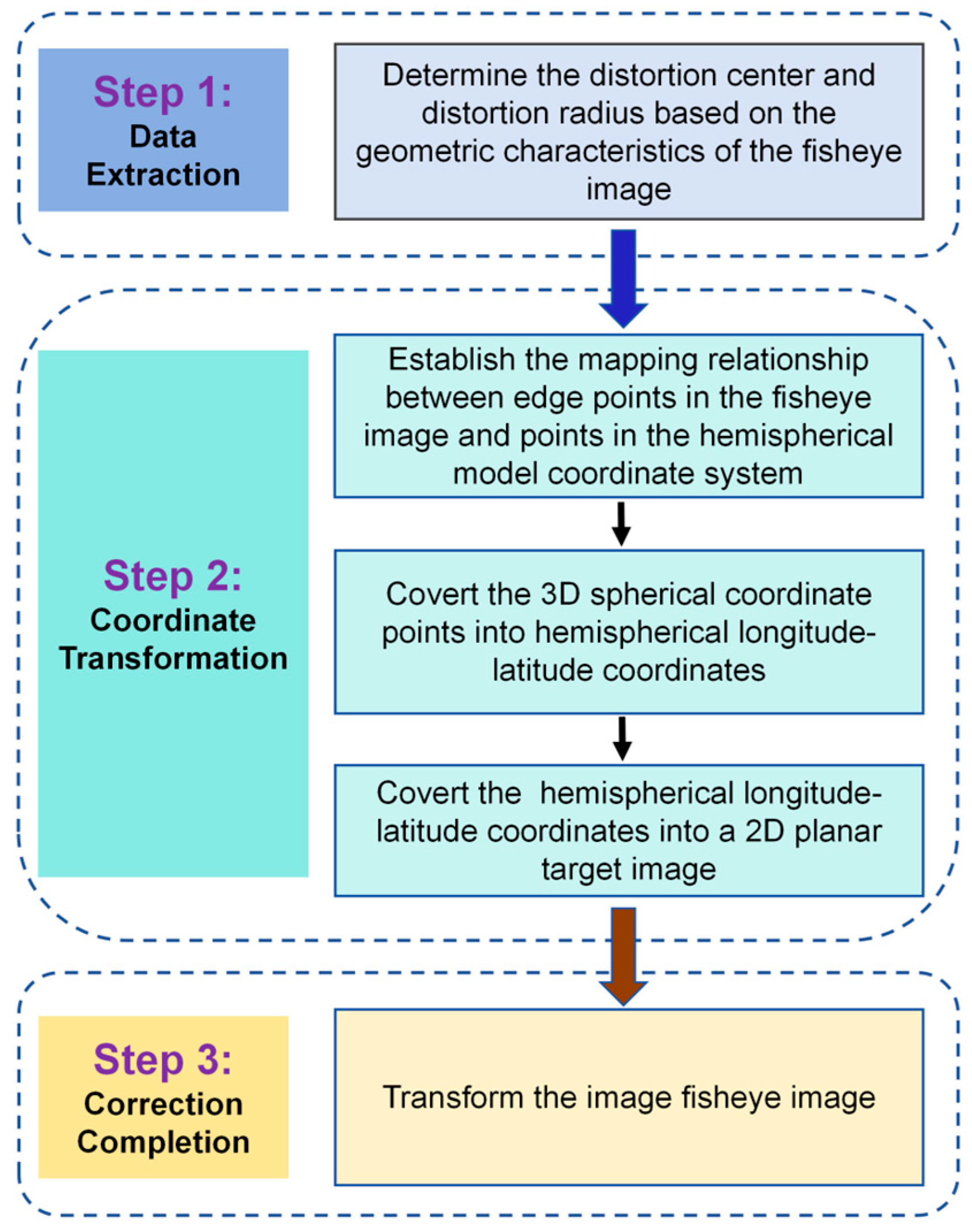
Fisheye cameras are widely used for ground-based cloud image acquisition because of their broad field of view and distinctive perspective projection. However, this wide-angle imaging characteristic often introduces deviations in the apparent size and position of objects in the captured image, with more pronounced distortion occurring near the image boundaries. The latitude–longitude mapping-based distortion correction algorithm is commonly adopted because it does not require external calibration equipment. By remapping each pixel in the image, the wide-angle view captured by the fisheye lens can be transformed into a standard perspective image that more closely resembles human visual perception, thereby improving both the visual quality and geometric accuracy of the image. The latitude–longitude fisheye correction algorithm consists of three main stages: data extraction, coordinate transformation, and image correction. The procedure is illustrated in Figure 1.

The correction procedure is described as follows. First, the distortion center and radius are determined based on the geometric characteristics of the fisheye image, which provides the basis for the subsequent correction process. A mapping is then established between the fisheye image coordinates and the coordinates of a hemispherical model, through which the fisheye image is projected onto the hemisphere and the corresponding spherical position of each image pixel is identified. Subsequently, the three-dimensional coordinates on the spherical surface are converted into spherical latitude–longitude coordinates and further mapped onto the two-dimensional coordinate system of the target planar image, thereby completing fisheye distortion correction. Through these geometric mappings and coordinate transformations, the curved structures caused by fisheye distortion can be rectified, and a distortion-corrected planar image can be obtained.

To improve the quality of the corrected image, enhance cloud features, and suppress noise, a gamma-based image enhancement method is employed. This method optimizes image quality by adjusting image brightness and contrast:

$$I_{out}=I^{\gamma }$$

(1)

where I denotes the distortion-corrected ground-based cloud image, and γ is the gamma coefficient, which typically ranges from 0 to 1.

2.1.2. Reducing Intraday Variations in Cloud Images

Because of variations in illumination intensity, meteorological conditions, and viewing angle, the pixel values of ground-based cloud images often exhibit pronounced temporal fluctuations. Histogram equalization is, therefore, applied to reduce intraday variations in cloud-image pixel values caused by changes in illumination.

Let r and s denote the input and output gray levels, respectively. The relationship between their probability density functions can be expressed as follows:

$$P_s(s)=P_r(r)·\left|{\displaystyle \frac{dr}{ds}}\right|, s=T\left(r\right)$$

(2)

where $P_r\left(r\right)$ and $P_s\left(s\right)$ denote the probability density functions of the input and output gray levels, respectively, and $T\left(·\right)$ represents the gray-level transformation function. For histogram equalization, the transformation function is defined by the cumulative distribution function of the input gray-level distribution:

$$s=T(r)={\displaystyle {\int }_0^r{p}_r(\omega )d\omega }$$

(3)

where ω is the integration variable. Assuming that the original image contains a total of n pixels and m gray levels, the equalized result $s_k$ at the k-th gray level can be written as follows:

$$s_k=T(r_k)={\displaystyle \sum _{j=0}^k{P}_r(r_j)={\displaystyle \sum _{j=0}^k\frac{n_j}{n}}} , 0\le r\le 1, k=0,1,\cdots ,m-1$$

(4)

where $T\left(r_k\right)$ denotes the pixel transformation function, $P_r\left(r_j\right)$ is the probability density of the j-th gray level, and $n_j$ is the number of pixels at the j-th gray level.

2.1.3. Solar Interference Suppression

In ground-based sky images, sunlit regions are prone to saturation, which can lead to cloud-detection errors. To reduce the influence of high-intensity solar regions on cloud detection, the pixel coordinates of the sun are first determined and then used to assess whether the image is affected by solar interference.

Because camera calibration data are unavailable, a solar pixel-coordinate localization model is constructed based on astronomical calculations and polynomial surface fitting, enabling accurate estimation of the solar position in ground-based sky images. Using the geographical and temporal metadata associated with image acquisition, the position of the sun in the horizontal coordinate system is calculated using astronomical formulas. The main parameters are the solar zenith angle (α) and the solar azimuth angle (β). Here, α denotes the angle between the incoming solar radiation and the zenith direction, while β denotes the angle between the projection of the sun on the horizontal plane and the due south direction. These two angles are calculated as follows:

$$\alpha =arccos(sin\delta sin\phi +cos\delta cos\phi cos\tau )$$

(5)

$$\beta =arccos({\displaystyle \frac{cos\alpha cos\phi sin\alpha sin\phi -sin\delta }{cos\alpha cos\phi }})$$

(6)

where δ is the solar declination angle calculated from the image acquisition date, ϕ is the geographical latitude of the imaging device, and τ is the solar hour angle jointly determined by the acquisition date, acquisition time, and device longitude. The solar hour angle represents the temporal offset of the sun relative to local noon.

By manually annotating sky images with clearly visible solar contours, the actual row–column pixel coordinates c of the solar center are extracted from each image to construct a solar-coordinate sample dataset. Because the mapping from the solar horizontal coordinates to the image-plane coordinates is nonlinear owing to fisheye projection and camera orientation, polynomial models of orders one to five were compared using the manually annotated solar-center samples. The polynomial order was selected according to the mean Euclidean pixel localization error obtained on the validation samples. The fifth-order model achieved the lowest validation error and provided a better representation of the nonlinear mapping near the image boundaries. Higher-order models were not considered because they would introduce additional coefficients and increase the risks of numerical instability and overfitting. Therefore, a fifth-order bivariate polynomial containing all terms satisfying $i+j\le 5$ was adopted. Let $c_r$ and $c_c$ denote the row and column coordinates of the solar center. A polynomial surface fitting model is then established using α and β as input variables and c as the output variable. The polynomial basis vector of α is defined as $\mathrm{Z}=[1,a,a^2,a^3,a^4,a^5]$, and that of β is defined as $A={[1,\beta ,{\beta }^2,{\beta }^3,{\beta }^4,{\beta }^5]}^{\mathrm{T}}$. The coordinate transformation can, therefore, be expressed as follows:

$$c=\left[\begin{array}{l}{c}_r\\ c_c\end{array}\right]=\left[\begin{array}{l}Z{P}^{\left(r\right)}A\\ Z{P}^{\left(c\right)}A\end{array}\right]$$

(7)

where $P^{\left(r\right)}$ and $P^{\left(c\right)}$ are the coefficient matrices obtained by fitting the annotated samples for the row and column coordinates, respectively. Equivalently, each coordinate can be expressed as follows:

$$c_q={\displaystyle \sum _{i=0}^5{\displaystyle \sum _{j=0}^{5-i}{p}_{ij}^{\left(q\right)}}}{\alpha }^i{\beta }^j, q\in \left\{r,c\right\}$$

(8)

where $p_{ij}^{\left(q\right)}$ denotes the optimal coefficient obtained by fitting the sample data, and $c_q$ represents the predicted row–column pixel coordinates of the solar center. To overcome the limitation that the blue channel in conventional RGB features is susceptible to saturation under intense solar illumination, an adjustable red–green difference (ARGD) feature is introduced. This feature model is constructed using only the red and green channels:

$$ARGD=k\times R-G$$

(9)

where k is the red-channel weighting coefficient, and R and G denote the grayscale values of the red and green channels of the image pixels, respectively. By dynamically adjusting k, the proposed feature enhances the pixel-level contrast between clouds and clear sky in high-intensity solar regions, thereby reducing the adverse influence of saturated pixels on feature representation. Solar intensity (SI) and saturation difference (SD) are then calculated to determine whether the image is affected by solar interference:

$$SI={\displaystyle \frac{{\displaystyle {\sum }_{i=1}^n{I}_i}}{n}}$$

(10)

$$SD={\displaystyle \frac{{\displaystyle {\sum }_{i=1}^{n_w}{S}_i}}{n_w}}-{\displaystyle \frac{{\displaystyle {\sum }_{j=1}^{n_1}{S}_j}}{n_1}}$$

(11)

where n is the number of pixels in the pixel block, $I_i$ is the grayscale value of the i-th pixel, $n_w$ is the total number of image pixels, $n_1$ is the number of pixels in the solar-center region, and $S_i$ and $S_j$ denote the saturation values of the corresponding pixels.

The solar intensity SI is a dimensionless integer ranging from 0 to 255 and represents the average brightness of the solar-center region. A high SI value generally indicates that the solar disk is visible and that the corresponding pixels approach saturation. The saturation difference SD is a dimensionless value ranging from 0 to 1 and characterizes the difference between the mean saturation of the entire sky image and that of the circumsolar region. A larger SD indicates a more nonuniform saturation distribution and a stronger influence of direct sunlight. The thresholds SI = 180 and SD = 0.1 were adopted from the sunlight-interference reduction method proposed. In Ref. [23], ground-based sky images were divided into four representative categories: overcast, cloudy without a visible sun, cloudy with a visible sun, and clear sky. The SI values of the overcast images without sunlight interference ranged from 28.81 to 176.92, and the corresponding SD values were below 0.08. Based on these statistical distributions, the thresholds were set to 180 and 0.1, respectively. An image is, therefore, considered free from sunlight interference only when both SI < 180 and SD < 0.1 are satisfied. If either SI ≥ 180 or SD ≥ 0.1, the image is classified as being affected by sunlight interference.

2.2. Ground-Based Cloud Image Feature Extraction

2.2.1. Cloud Coverage

Cloud coverage characterizes the extent to which the solar radiation received by photovoltaic panels is affected at the current moment, as well as the short-term variation trend of cloud cover. To separate cloud regions from sky regions, gray-scale thresholding is commonly used to convert a gray-scale image into a binary image. The cloud coverage parameter can be defined as the ratio of cloud-region pixels to the total number of pixels in the binary image:

$$CV={\displaystyle \frac{{\displaystyle \sum _{i,j}^{m,n}B\left(i,j\right)}}{m\times n}}$$

(12)

where m and n denote the height and width of the image, respectively. $B\left(i,j\right)$ follows the binarization rule: $B\left(i,j\right)=1$ when the gray-scale value of the pixel is greater than or equal to the threshold T, and $B\left(i,j\right)=0$ otherwise. Threshold selection is critical for image segmentation. The maximum inter-class variance method can optimize threshold selection and achieve effective object segmentation for different types of images. In this study, the processed ground-based sky images were represented as 8-bit grayscale images. For a gray-scale ground-based cloud image with $L=2^8=256$ gray levels, let $n_i$ denote the number of pixels with gray level i, and let N denote the total number of pixels. Then, $P_i$ represents the occurrence probability of gray level i. When the original cloud image is divided by threshold T into two classes, namely the background region and the target region, the occurrence probabilities of the two classes, denoted as $P_b$ and $P_o$, are obtained by summing the probabilities of the corresponding gray levels within each region. The gray-scale mean values of the background and target regions are expressed as follows:

$${\mu }_b={\displaystyle \frac{{\displaystyle \sum _{i=1}^T{n}_i\times i}}{{\displaystyle \sum _{i=1}^T{n}_i}}}={\displaystyle \frac{{\displaystyle \sum _{i=1}^T{P}_i\times i}}{P_b}}$$

(13)

$${\mu }_o={\displaystyle \frac{{\displaystyle \sum _{i=T+1}^L{n}_i\times i}}{{\displaystyle \sum _{i=T+1}^L{n}_i}}}={\displaystyle \frac{{\displaystyle \sum _{i=T+1}^L{P}_i\times i}}{P_o}}$$

(14)

The between-class variance of the background and target regions in the original image is given by the following:

$$D\left(T\right)=P_b{P}_o{\left({\mu }_b-{\mu }_o\right)}^2$$

(15)

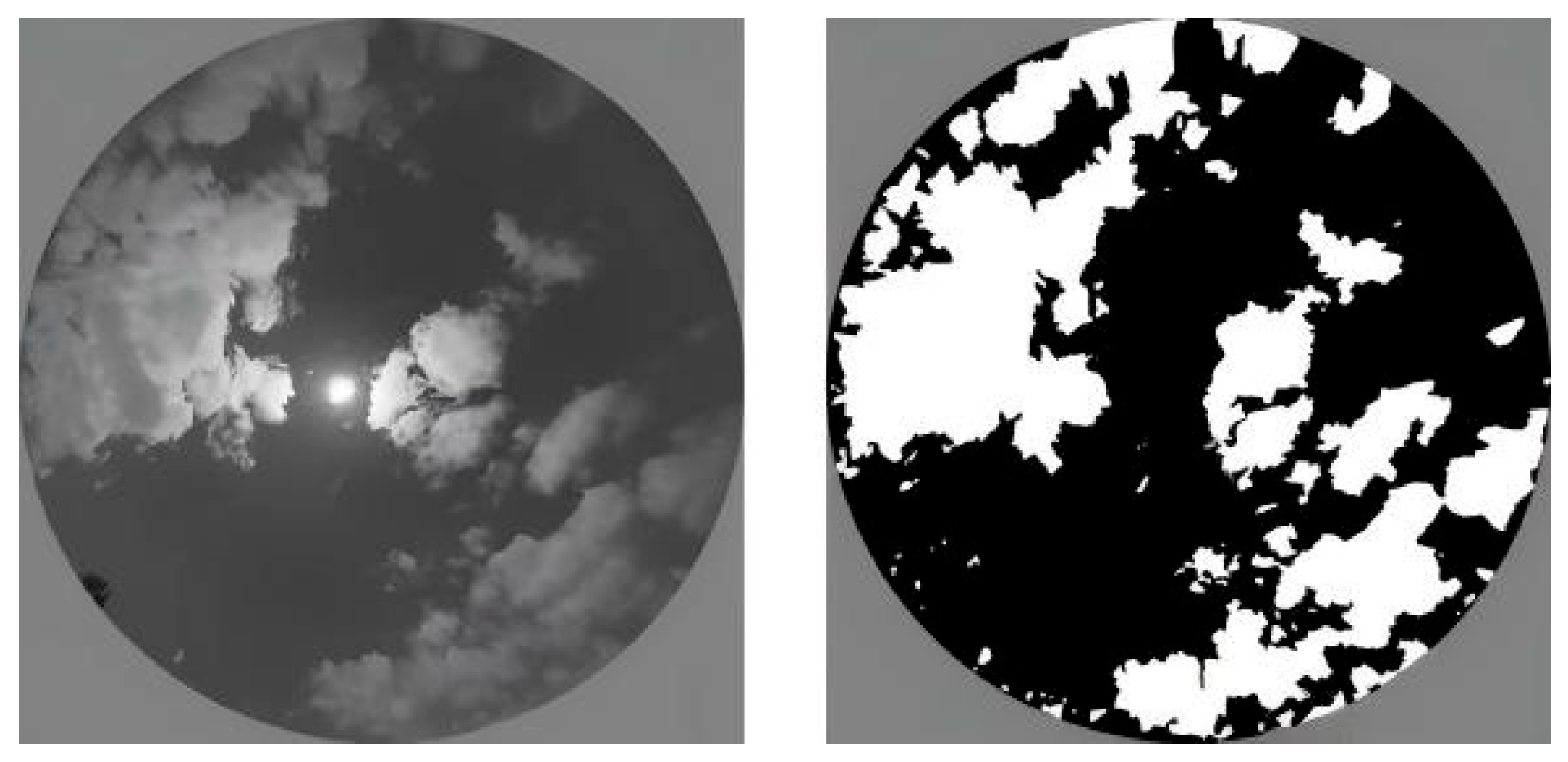
The threshold T that satisfies condition $\underset{1\le T\le L}{\max }\left[D\left(T\right)\right]$ is the optimal threshold for segmenting the background and target regions. This optimal threshold is then substituted into the cloud-coverage Equation (11) to calculate the cloud coverage at the current time instant. The cloud segmentation result is shown in Figure 2, where the white regions represent clouds and the black regions represent the sky. For the representative image shown in Figure 2, the cloud coverage calculated after solar-interference suppression was 34.18%. When the solar-interference suppression step was omitted, saturated pixels in the circumsolar region were incorrectly classified as cloud pixels, resulting in an estimated cloud coverage of 39.36%. Therefore, the absence of solar-interference suppression caused a relative overestimation of 15.16%. This case comparison demonstrates that solar-interference suppression can effectively reduce false cloud detection around the solar region and improve the reliability of the extracted cloud-coverage feature.

2.2.2. Cloud Motion Features

Because cloud formation and dissipation are dynamic processes, the motion features of cloud regions in ground-based cloud images need to be extracted. Optical flow describes the pixel-wise motion between consecutive frames in an image sequence. Specifically, from frame t to frame t + 1, the motion velocity and direction of each pixel together characterize its optical-flow feature. Suppose that a pixel is located at $\left(x,y\right)$ at time t. After a time interval $d_t$, its displacement between two adjacent frames can be represented by $d_x$ and $d_y$. The optical-flow constraint equation is, therefore, expressed as follows:

$$I\left(x,y,t\right)=I\left(x+dx,y+dy,t+dt\right)$$

(16)

where $I\left(x,y,t\right)$ denotes the intensity value of pixel $\left(x,y\right)$ at time t. If the displacement during dt is sufficiently small, a Taylor expansion around $\left(x,y,t\right)$ can be written as follows:

$$I\left(x+dx,y+dy,t+dt\right)=I\left(x,y,t\right)+{\displaystyle \frac{\partial I}{\partial x}}dx+{\displaystyle \frac{\partial I}{\partial y}}dy+{\displaystyle \frac{\partial I}{\partial t}}dt+R_n\left(x,y,t\right)$$

(17)

where $R_n\left(x,y,t\right)$ denotes the higher-order remainder term, which is approximately zero and can, therefore, be neglected. Thus, the above equation can be simplified as follows:

$$I_x{v}_x+I_y{v}_y=-I_t$$

(18)

where $I_x$, $I_y$, and $I_t$ denote the partial derivatives of $I\left(x,y,t\right)$ with respect to x, y, and t, respectively. $v_x$ and $v_y$ denote the velocity components of the pixel in the x- and y-directions, respectively.

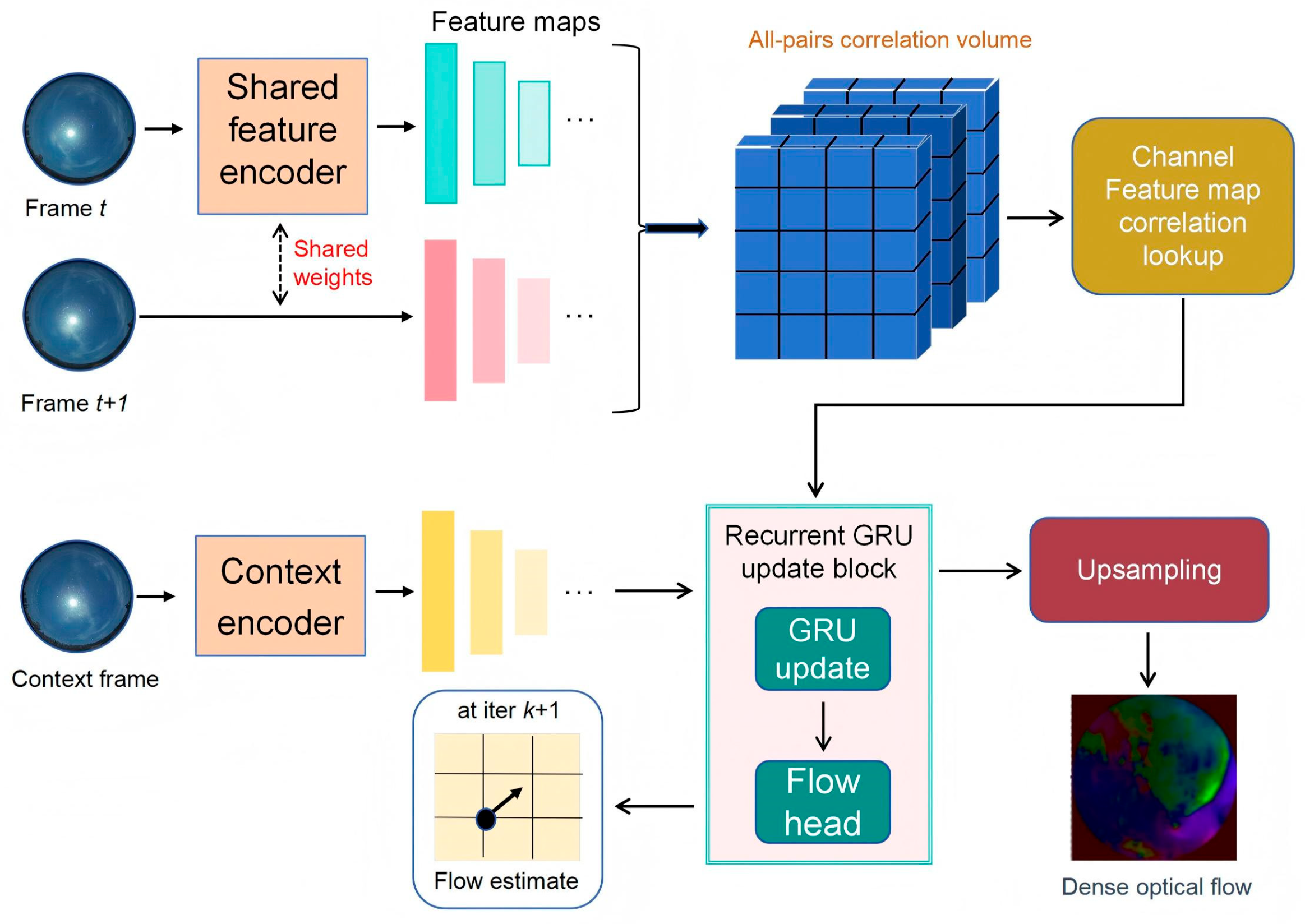
To improve the accuracy of optical-flow estimation, the deep-neural-network-based Recurrent All-Pairs Field Transforms (RAFT) optical flow method is employed to extract the motion direction and velocity of cloud regions. RAFT iteratively refines optical-flow estimates using a recurrent neural network. It performs particularly well for small objects and fast-moving objects while maintaining high computational efficiency and strong generalization capability. The RAFT network architecture is shown in Figure 3.

The RAFT network is composed of three modules. First, the feature encoder employs multiple convolutional layers to extract features from two consecutive image frames. Next, the correlation module constructs a 4D correlation volume by computing the inner products between the feature vectors of the two frames. Average pooling is then applied over the last two dimensions to generate feature representations at different scales, thereby forming a multi-scale correlation pyramid. Subsequently, convolution operations are used to extract correlation features for the following stages. Finally, the optical flow decoder iteratively estimates the optical flow. During this process, RAFT incorporates a gated recurrent unit to update the optical-flow state, and the resulting output is passed through two convolutional layers to produce the optical-flow estimate for the current iteration. The results from all iterations are progressively aggregated to obtain the final optical flow field.

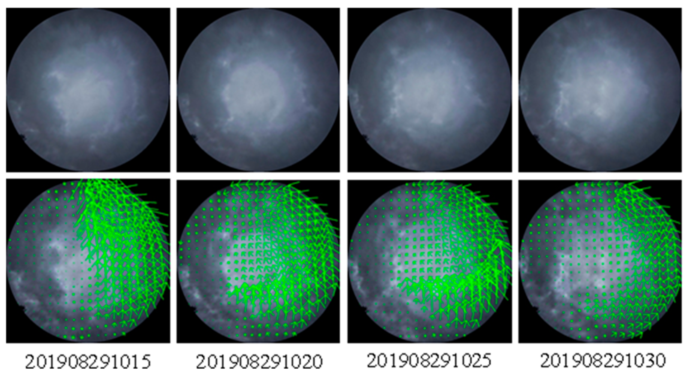
To visualize the motion of cloud clusters, green arrows are used to represent sparse motion vectors on images with a resolution of 1024 × 1024, with one arrow plotted at every 50-pixel interval. The arrow direction indicates the direction of cloud motion, while the arrow length is proportional to the cloud motion speed. Thus, faster cloud motion corresponds to longer arrows. As shown in Figure 4, the displacement of cloud clusters in ground-based cloud images at consecutive time steps is illustrated. Because optical-flow vectors represent pixel displacement rather than absolute physical cloud velocity, the vectors were converted into resolution- and time-normalized image-plane motion features. First, only the vectors located within the cloud region, obtained from the cloud-segmentation mask, were retained. Clear-sky pixels and invalid background regions were excluded. The representative horizontal and vertical displacements of the cloud field were calculated using the median of the valid cloud-pixel vectors to reduce the influence of local estimation noise and abnormal motion vectors. The displacement components were subsequently normalized according to the image resolution and temporal interval. The cloud’s movement direction is determined by calculating the normalized horizontal and vertical cloud velocities using trigonometric functions. Therefore, the dynamic cloud-image inputs consisted of the normalized motion magnitude and the directional components. Before model training, the motion magnitude was standardized using the mean and standard deviation obtained exclusively from the training set, and the same transformation was applied to the validation and test sets.

To further explore the impact of image preprocessing on cloud motion extraction, continuous images under strong light interference were selected and analyzed under three configurations: the original fisheye images, the distortion-corrected images, and the images processed using both distortion correction and solar-interference suppression. The proportion of locally inconsistent optical-flow vectors decreased from 13.2% for the original images to 8.1% after distortion correction and further decreased to 4.8% after solar-interference suppression. Meanwhile, the standard deviation of the cloud-motion direction decreased from 28.6° to 21.3° and 16.9°, respectively. The normalized mean motion magnitude changed from 3.8 × 10⁻³ to 3.4 × 10⁻³ and 3.2 × 10⁻³ image widths per minute. These results indicate that distortion correction reduces artificial motion caused by fisheye deformation near the image boundaries, whereas solar-interference suppression reduces abnormal high-magnitude vectors and direction fluctuations around the circumsolar region. Consequently, the preprocessed images provide a more spatially coherent optical-flow field for extracting cloud-motion magnitude and direction.

2.3. Deep Learning Model

2.3.1. CNN

Convolutional neural networks (CNNs) are representative deep learning models. By exploiting local connections, weight sharing, and pooling operations, CNNs can efficiently extract features while substantially reducing the number of network parameters and the dimensionality of data, thereby improving computational efficiency and feature representation capability.

The convolutional layer is a core component of CNNs and is used to extract features from input data at different levels. If the output of the convolution operation is an $L^{\ast }\times W^{\ast }$ matrix O, the convolutional layer can be formulated as follows:

$$O(i,j)=f\left({\displaystyle \sum _{d=0}^D{\displaystyle \sum _{l=0}^{L\prime }{\displaystyle \sum _{w=0}^{W\prime }I\left(S\ast i+l,S\ast j+w,d\right)}}}\ast K(l,w,d)+b\right)$$

(19)

where $O\left(x,y\right)$ denotes the element at coordinate $\left(x,y\right)$ in the output matrix O; $I\left(x,y,z\right)$ and $K\left(x,y,z\right)$ denote the elements at coordinate $\left(x,y,z\right)$ in the input matrix I and convolution kernel K, respectively; S denotes the stride of the convolution kernel; b is the bias term and f(⋅) represents the activation function.

Although convolutional layers can extract rich features from the input data, these features may contain substantial similarity, redundancy, or noise. Pooling layers reduce the spatial dimensionality of feature maps and decrease the number of network parameters. In doing so, they retain key features while accelerating computation and mitigating overfitting.

The fully connected layer integrates the local features extracted by the convolutional and pooling layers into global representations, thereby performing classification or regression on the input data. Through the backpropagation algorithm, the network learns high-level features from the input data and continuously optimizes the parameters of the fully connected layer.

2.3.2. Autoformer

The attention mechanism has been widely used in deep learning. By leveraging attention, the Transformer architecture can effectively model dependencies among sequence elements while offering strong parallel computing capability. However, its self-attention mechanism has quadratic computational complexity and high memory consumption, which leads to degraded performance when handling long time series. To address these limitations, Autoformer builds upon the Transformer architecture by improving both sequence decomposition and the self-attention mechanism, and introduces a deep decomposition architecture together with an autocorrelation mechanism.

(1)

Sequence decomposition architecture

The Autoformer model embeds a sequence decomposition mechanism into both the encoder and decoder modules, thereby forming a deep decomposition structure. During forecasting, the model alternates between decomposition and refinement, gradually extracting trend and periodic components to achieve a hierarchical and progressive sequence modeling process. The sequence decomposition unit employs an adjustable moving-average mechanism to smooth periodic fluctuations in the sequence and thereby emphasize the long-term trend. For an input sequence X of length L, the decomposition process is given by:

$$X_t=\mathrm{AvgPool}\left(\mathrm{Padding}\left(X\right)\right)$$

(20)

$$X_s=X-X_t$$

(21)

where $X_t$ denotes the seasonal component, $X_s$ denotes the trend component extracted from the sequence, AvgPool(⋅) denotes average pooling for moving-average processing, and Padding denotes padding around the boundaries of the input data.

(2)

Autocorrelation mechanism

Time-series data generally exhibit periodicity, and subsequences from similar positions often show similar patterns. Based on this property, Autoformer introduces an autocorrelation mechanism to establish efficient sequence-level dependencies and enhance the model’s ability to extract temporal information. By calculating the autocorrelation coefficients of the sequence, the model identifies potential periodic dependency patterns. Combined with a time-delay aggregation operation, structurally similar subsequences can be effectively integrated, thereby improving information transmission as well as forecasting accuracy and efficiency. For the input sequence X, if similar subsequences exist with a period of τ, the autocorrelation coefficient can be calculated as follows:

$$R_{XX}\left(\tau \right)=\underset{L\to \infty }{\lim }{\displaystyle \frac{1}{L}}{\displaystyle \sum _{t=0}^{L-1}{X}_t{X}_{t-\tau }}$$

(22)

where $R_{XX}\left(\tau \right)$ denotes the lagged similarity between the discrete time series and its sequence delayed by τ, and L denotes the number of delay operations.

2.3.3. CNN-Autoformer

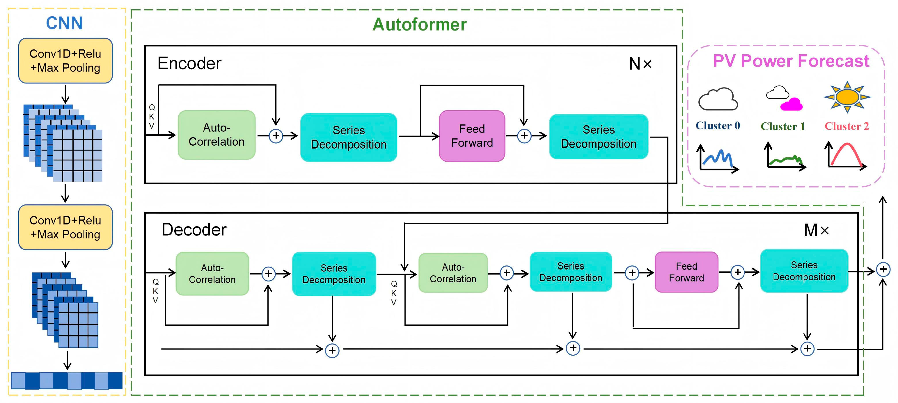
To improve the accuracy of ultra-short-term photovoltaic power forecasting, this study develops a hybrid CNN–Autoformer model that integrates meteorological variables, historical photovoltaic power, and the static and dynamic features extracted from ground-based sky images, as illustrated in Figure 5. Each input sample contains 36 consecutive observations with a temporal resolution of 5 min, corresponding to a historical window of 180 min. A direct multi-step forecasting strategy is adopted, through which the model simultaneously predicts photovoltaic power at the subsequent 5, 10, and 15 min horizons.

The CNN module is first employed to extract local temporal patterns from the multivariate input feature matrix. It contains two one-dimensional convolutional layers with 64 and 96 filters, respectively. Both convolutional layers use a kernel size of 3, a stride of 1, and a padding size of 1, followed by a ReLU activation function and a max-pooling layer with a kernel size of 2 and a stride of 2. Through the two convolution–pooling blocks, the temporal sequence length is progressively reduced from 36 to 18 and then to 9, while short-term variations and interactions among the input variables are retained in a compact feature representation. The resulting feature sequence is subsequently projected into a 96-dimensional latent space and supplied to the Autoformer module. The Autoformer consists of two encoder layers and two decoder layers. Each layer uses four autocorrelation heads, corresponding to a feature dimension of 24 per head, while the feed-forward network dimension is set to 384. In the encoder, the autocorrelation mechanism calculates sequence-level temporal dependencies in the frequency domain using the fast Fourier transform and aggregates the dominant time delays. The series-decomposition module then separates the latent sequence into trend and seasonal components using a moving-average window of 7. This decomposition and refinement procedure is repeated progressively across the encoder layers, enabling the model to characterize both the overall variation trend and recurrent temporal patterns of photovoltaic power. The decoder further processes the forecasting sequence through self-autocorrelation and encoder–decoder autocorrelation operations. The former captures the internal temporal relationships within the decoder input, while the latter incorporates the contextual information extracted by the encoder. Series decomposition is embedded after the autocorrelation and feed-forward operations, allowing the seasonal and trend information to be progressively refined. Finally, the decoder outputs corresponding to the future time steps are mapped through a linear regression layer to generate photovoltaic power forecasts for the next 5, 10, and 15 min. A dropout rate of 0.12 is applied to reduce overfitting. By combining the local pattern-extraction capability of the CNN with the progressive series decomposition and autocorrelation mechanisms of Autoformer, the proposed model can simultaneously capture rapid short-term fluctuations, overall trend variations, and temporal dependency patterns in photovoltaic power sequences. This architecture is, therefore, particularly suitable for ultra-short-term forecasting scenarios in which photovoltaic output is strongly affected by rapidly evolving cloud cover and cloud motion.

For model training, the batch size is 256, and the maximum number of training epochs is 120. The AdamW optimizer is adopted with an initial learning rate of 8 × 10⁻⁴ and a weight-decay coefficient of 1 × 10⁻⁴. Smooth L1 loss with β = 0.5 is used as the objective function. In addition, a ReduceLROnPlateau learning-rate scheduler is employed with a reduction factor of 0.5 and a patience of 5 epochs. Early stopping is applied according to the validation loss, and training is terminated if the validation loss does not improve by more than 1 × 10⁻⁶ for 20 consecutive epochs.

2.3.4. Similar-Day Clustering

Clustering is a typical unsupervised learning method that identifies intrinsic patterns and feature distributions from unlabeled samples. In this study, the K-means clustering method is used to classify the daily weather conditions. Each sample is assigned to only one cluster, and the dataset is partitioned into a predefined number of K clusters by minimizing the Euclidean distance between each sample and its assigned cluster centroid. Owing to its algorithmic simplicity, ease of implementation, and good scalability, K-means is suitable for processing large-scale photovoltaic output datasets.

To group historical samples with similar photovoltaic generation patterns, the K-means clustering algorithm was applied to the daily photovoltaic power profiles. Instead of directly classifying weather conditions using individual meteorological variables, the clustering procedure was based on three statistical characteristics extracted from each daily power curve: the daily mean photovoltaic output, the number of power fluctuations, and the magnitude of the power fluctuations. The daily mean output reflects the overall solar-energy availability, whereas the fluctuation frequency and magnitude characterize short-term power variations caused primarily by intermittent cloud shading.

The number of clusters was set to K = 3 to distinguish three representative photovoltaic operating patterns. After clustering, the meteorological labels were assigned according to the characteristics of the cluster centroids. The cluster with a high daily mean power output and relatively low fluctuation frequency and magnitude was labeled as sunny. The cluster with a relatively high output level but frequent and pronounced power fluctuations was labeled as cloudy, because intermittent cloud movement and shading generally lead to rapid increases and decreases in photovoltaic generation. The cluster with a low daily mean output and relatively weak fluctuations was labeled as overcast, representing persistent cloud coverage and continuously reduced solar irradiance. Therefore, the weather labels were assigned after clustering based on the physical interpretation of the photovoltaic power patterns rather than being specified as supervised labels in advance. After temporal synchronization, preprocessing, and data-quality filtering, a total of 49,972 valid samples were retained, including 15,860 sunny samples, 19,540 cloudy samples, and 14,572 overcast samples.

3. Results and Discussions

3.1. Baseline Data

The dataset used in this study covers the period from 1 June to 26 October 2019. All ground-based sky images and photovoltaic power measurements were obtained from the original 2019 release of the SKIPP’D dataset [24]. The sky camera and the 30.1 kW-DC rooftop photovoltaic array were both located on the Stanford University campus at approximately 37.43° N, 122.17° W, with a separation distance of approximately 125 m. The sky-image and photovoltaic-power data streams were recorded using synchronized local clocks at an original temporal resolution of 1 min, thereby ensuring that the observed cloud conditions were spatially and temporally representative of the photovoltaic system.

The meteorological variables, including temperature, relative humidity, wind speed, and global horizontal irradiance, were obtained from the National Solar Radiation Database (NSRDB). The dataset was accessed via the NSRDB Data Viewer (https://nsrdb.nlr.gov/). The meteorological data were retrieved by specifying the geographical coordinates of the Stanford study site, the year 2019, and a temporal resolution of 5 min. The corresponding NSRDB data have a temporal resolution of 5 min and a spatial resolution of approximately 2 km. To construct a temporally consistent multimodal dataset, the original 1 min sky-image and photovoltaic-power records were manually screened and subsampled onto a common 5 min time grid. For each NSRDB timestamp, the nearest available sky image and photovoltaic-power measurement were selected, and only samples with an absolute timestamp difference of less than 1 min were retained. The extracted static and dynamic cloud-image features were subsequently combined with the meteorological variables and historical photovoltaic power measurements as model inputs. Because the photovoltaic system produces no power at night, only observations collected between 06:00 and 20:00 each day were retained.

For each weather category, the dataset was divided chronologically at the daily level. The earliest 80% of the days were assigned to the training set, the subsequent 10% to the validation set, and the latest 10% to the test set. All 5-min observations from the same day were retained in the same subset. Input–output sequences were constructed independently within each subset, and sequences crossing dataset boundaries were discarded. The normalization parameters were calculated using only the training set and were subsequently applied to the validation and test sets. Random shuffling was used only for training mini-batches after the chronological partition, thereby preventing temporal information leakage among the three datasets. To meet the requirements of ultra-short-term power forecasting for distributed photovoltaic generation, a direct multi-step forecasting strategy is adopted. The forecasting horizon is set to three steps, with a temporal resolution of 5 min. Therefore, based on current and historical observations, the model simultaneously outputs the predicted power values for the next 5, 10, and 15 min, thereby predicting the complete output trajectory over the following 15 min. The 5-min temporal resolution is sufficient to capture minute-level power fluctuations caused by cloud motion, while the 15-min forecasting horizon aligns with the decision-making window required for ultra-short-term dispatch and real-time control of distributed photovoltaic systems. Accordingly, the reported evaluation metrics are calculated by equally aggregating the predicted and actual values at the 5-, 10-, and 15-min horizons. These metrics, therefore, represent the overall forecasting performance of the complete three-step power trajectory.

The experiments were performed using an Intel(R) Core(TM) i5-12600F CPU, an NVIDIA GeForce RTX 5060 GPU with 8 GB of graphics memory, and 16 GB of system memory. The implementation was developed in Python 3.10.12 using PyTorch 2.5.0 and CUDA 12.4.0. The proposed model required approximately 10 min for offline training, while the complete online inference procedure required approximately 2 min per forecasting cycle. Since the inference time was shorter than the 5 min data-update interval, the proposed method could complete the forecasting process before the next observation became available, supporting its suitability for real-time ultra-short-term photovoltaic power forecasting.

To evaluate the performance of the proposed CNN-Autoformer model in ultra-short-term photovoltaic power forecasting, comparative ablation experiments are designed. Four models, namely CNN, Transformer, Autoformer, and CNN-Transformer, are selected for comparison. To ensure the reproducibility and fairness of the model comparison, all experiments were conducted using a fixed random seed. All models use the same data partitioning scheme, input variables, training strategy, and evaluation metrics to ensure a fair comparison.

3.2. Evaluation Metrics

To evaluate the forecasting performance of the model, four commonly used evaluation metrics are adopted: root mean square error (RMSE), mean absolute error (MAE), normalized mean absolute error (nMAE) and the coefficient of determination (R²). These metrics are used to quantitatively assess the prediction results, and their calculation formulas are given as follows:

$$\mathrm{RMSE}=\sqrt{{\displaystyle \frac{1}{N}}{\displaystyle \sum _{i=1}^N{\left(Y_p-Y_{\mathrm{t}}\right)}^2}}$$

(23)

$$\mathrm{MAE}={\displaystyle \frac{1}{N}}{\displaystyle \sum _{i=1}^N\left|Y_p-Y_t\right|}$$

(24)

$$\mathrm{nMAE}={\displaystyle \frac{\mathrm{MAE}}{P_{\mathrm{rated}}}}\times 100\%$$

(25)

$${\mathrm{R}}^2=1-{\displaystyle \frac{{\displaystyle \sum _{i=1}^N{\left(Y_t-Y_{\mathrm{p}}\right)}^2}}{{\displaystyle \sum _{i=1}^N{\left(Y_t-\frac{1}{N}{\displaystyle \sum _{i=1}^N{Y}_{\mathrm{t}}}\right)}^2}}}$$

(26)

where N denotes the number of samples in the dataset, $Y_t$ represents the actual photovoltaic output, and $Y_p$ represents the model-predicted photovoltaic output, and where $P_{\mathrm{rated}}$ denotes the rated DC capacity of the photovoltaic array, which is 30.1 kW-DC.

3.3. Prediction Result Comparison Analysis

As shown in

Table 1. Evaluation metrics for model predictions under different weather conditions.

Model	Weather Type	RMSE/kW	MAE/kW	R2/%
CNN	Sunny	1.665	1.247	92.99
	Cloudy	5.111	3.851	61.31
	Overcast	3.649	3.101	78.21
Transformer	Sunny	1.733	1.323	91.74
	Cloudy	4.965	3.259	65.33
	Overcast	3.079	2.603	81.71
Autoformer	Sunny	0.9700	0.718	97.43
	Cloudy	4.829	3.338	65.52
	Overcast	2.079	1.357	85.79
CNN-Transformer	Sunny	1.568	1.290	93.95
	Cloudy	4.512	3.299	69.51
	Overcast	2.264	1.811	83.70
CNN-Autoformer	Sunny	0.576	0.392	98.01
	Cloudy	3.266	2.669	74.61
	Overcast	1.514	1.051	91.57

, CNN-Autoformer achieves the lowest RMSE and MAE and the highest R² across the three weather conditions, indicating that the proposed model provides superior forecasting accuracy and robust generalization under different weather scenarios. Under sunny conditions, the photovoltaic power curve is generally smooth, and Autoformer can effectively extract the trend and periodic components of the power sequence. Compared with Autoformer, CNN-Autoformer reduces RMSE and MAE by 40.62% and 45.40%, respectively, while increasing R² by 0.58%. This demonstrates that the local feature extraction structure of the CNN further enhances the model’s ability to capture subtle local fluctuations under sunny conditions.

Under overcast conditions, photovoltaic power is affected by cloud shading and irradiance variations, resulting in greater volatility in the output curve. The RMSE, MAE, and R² of CNN-Autoformer are 1.514 kW, 1.051 kW, and 91.57%, respectively. Compared with Autoformer, CNN-Autoformer reduces RMSE by 27.18% and MAE by 22.55%, while improving R² by 5.78%. These results indicate that the sequence decomposition and autocorrelation mechanisms of Autoformer alone can capture the overall variation trend, but remain insufficient for modeling local fluctuations. By incorporating the CNN, the model can more effectively extract local variation features over short timescales, thereby improving forecasting accuracy under overcast conditions.

Under cloudy conditions, cloud movement and shading variations occur more frequently, leading to stronger non-stationarity and abrupt fluctuations in photovoltaic power. In this scenario, CNN-Autoformer achieves an RMSE of 3.266 kW, an MAE of 2.669 kW, and an R² of 74.61%. Compared with CNN-Transformer, the best-performing baseline in terms of RMSE, CNN-Autoformer reduces RMSE by 27.62% and improves R² by 5.10%. Compared with Transformer, which performs better in terms of MAE, CNN-Autoformer reduces MAE by 18.10%. These results show that CNN-Autoformer can simultaneously exploit the ability of the CNN to extract local short-term fluctuations and the capability of Autoformer to model trend components, periodic components, and long-term dependencies. As a result, the proposed model exhibits stronger adaptability in cloudy scenarios with frequent cloud variations.

Overall, the model comparison experiments show that CNN-Autoformer outperforms CNN, Transformer, Autoformer, and CNN-Transformer across different weather conditions, demonstrating the effectiveness of the proposed hybrid architecture.

However, forecasting performance depends not only on the network structure but also on how effectively the input data characterize the mechanisms driving photovoltaic power fluctuations. The role of the extracted cloud-image features in photovoltaic power forecasting is further clarified here. The proposed CNN–Autoformer does not directly use raw sky images as model inputs. Instead, the processed ground-based sky images are converted into physically interpretable numerical features, including cloud coverage, normalized cloud-motion magnitude, and motion-direction components, as described in Section 2. These cloud-image features are temporally aligned with the meteorological variables and historical photovoltaic power measurements to construct a multivariate time-series input. Specifically, cloud coverage characterizes the instantaneous cloud-shading condition, whereas the cloud-motion features describe the short-term evolution of the cloud field. Together with meteorological conditions and historical PV power, these variables provide complementary information for characterizing the factors associated with short-term photovoltaic power fluctuations. Therefore, in the following analysis, CNN-Autoformer is used as the fixed forecasting model, and different input feature combinations are constructed for further comparison under sunny, cloudy, and overcast conditions. This enables a quantitative evaluation of the effects of static cloud-image features, dynamic cloud-image features, and their fusion on ultra-short-term photovoltaic power forecasting. The feature combinations are defined as follows:

• Feature 1: meteorological data and historical power data;
• Feature 2: meteorological data and historical power data + static cloud-image features, including cloud cover;
• Feature 3: meteorological data and historical power data + dynamic cloud-image features, including cloud velocity and direction;
• Feature 4: meteorological data and historical power data + static cloud-image features, including cloud cover + dynamic cloud-image features, including cloud velocity and direction.

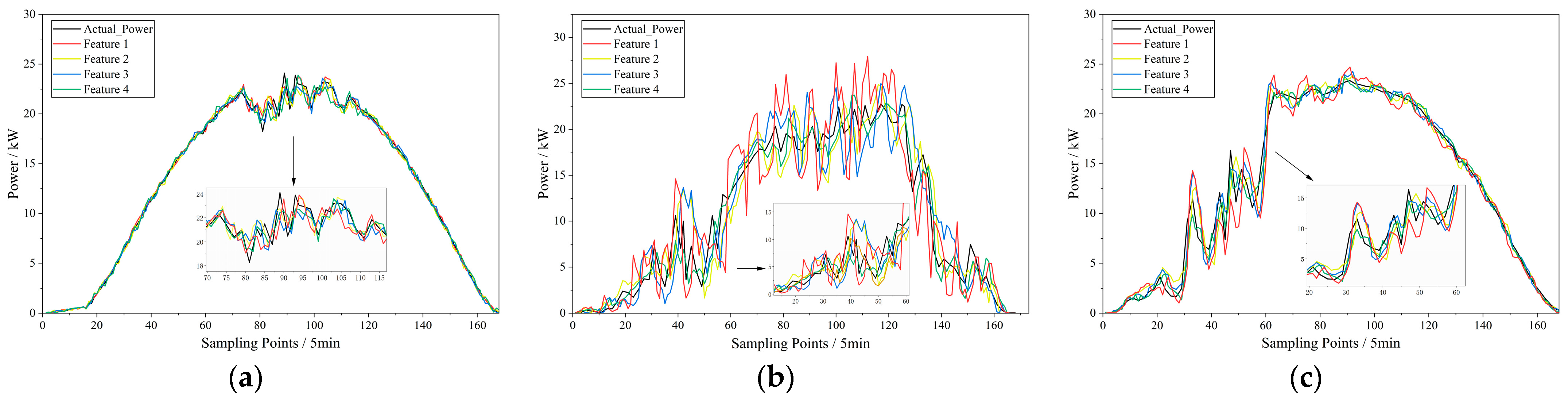
The forecasting results obtained with different input feature combinations are shown in Figure 6. Under sunny conditions, the photovoltaic power curve is generally smooth, and all four feature combinations can effectively track the actual power variation trend. However, the zoomed-in view shows that Feature 1, which uses only meteorological data and historical power data, still exhibits certain deviations in local fluctuation intervals, whereas the prediction curve of Feature 4 is closest to the actual power curve. Under cloudy conditions, the power curve exhibits the strongest fluctuations, and the differences among the feature combinations become most pronounced. Feature 1 relies only on meteorological and historical power data, and therefore, shows limited responsiveness to rapid power increases and decreases, resulting in relatively large deviations from the actual fluctuation pattern. After static or dynamic cloud-image features are introduced, the prediction curves become noticeably closer to the actual values. Among all feature combinations, Feature 4 achieves the best tracking performance in peak, valley, and rapidly fluctuating intervals, showing the strongest agreement with the actual curve. Under overcast conditions, photovoltaic power is generally affected by cloud shading, and the fluctuation amplitude lies between those observed under sunny and cloudy conditions. Feature 4 still exhibits the best tracking capability, especially in local fluctuation intervals, where its prediction curve is smoother and more consistent with the actual power variation trend.

Table 2. Evaluation metrics for prediction results based on different features under clear weather conditions.

Feature	RMSE/kW	MAE/kW	nMAE/%	R2/%
feature 1	0.576	0.392	1.30	98.01
feature 2	0.459	0.313	1.04	98.83
feature 3	0.519	0.365	1.21	98.38
feature 4	0.369	0.264	0.88	99.52

presents the evaluation metrics for the four input feature combinations under sunny weather conditions. Feature 4 achieves the best forecasting performance. Feature 4 reduced the nMAE from 1.30% to 0.88% compared with Feature 1, a decrease of approximately 32.65%. A further comparison between Feature 2 and Feature 3 shows that incorporating static cloud-image features leads to better prediction results than incorporating dynamic cloud-image features. This is mainly because cloud cover is relatively limited under sunny conditions, and photovoltaic power variations are comparatively smooth. In this case, the current cloud-cover state provides a more direct representation of power variations, whereas cloud-motion features contribute relatively limited additional improvement.

Under sunny weather conditions, photovoltaic output is relatively stable, while multi-feature fusion is more effective for complex time-series scenarios. Therefore, the improvement in forecasting performance is limited, and the advantages of feature fusion are not fully exploited. To quantify the relative importance of the input variables under different weather conditions, a block-permutation feature-importance analysis was performed using the trained CNN–Autoformer and the chronologically separated test set. The adopted analysis evaluates the dependence of the forecasting model on each input feature by measuring the increase in prediction error after that feature is disrupted. Let $E_0$ denote the RMSE calculated from the original test data. For the j-th input feature, the feature values were permuted in complete daily blocks within the same weather category, while the remaining input features and the trained model parameters were kept unchanged. The RMSE obtained from the b-th permutation was denoted by $E_{\mathrm{j}}^{(b)}$. The raw importance of the j-th feature was calculated as follows:

$$I_j={\displaystyle \frac{1}{B}}{\displaystyle \sum _{b=1}^B\frac{E_j^{\left(b\right)}-E_0}{E_0}}$$

(27)

where B is the number of independent permutation repetitions. A larger $I_j$ indicates that disrupting the corresponding feature causes a greater deterioration in forecasting performance and that the trained model exhibits a stronger dependence on this feature. To facilitate comparison among input variables, the importance scores were further normalized as follows:

$$C_j={\displaystyle \frac{\max \left(I_{\mathrm{j}},0\right)}{{\displaystyle {\sum }_{k=1}^d\max \left(I_k,0\right)}}}\times 100\%$$

(28)

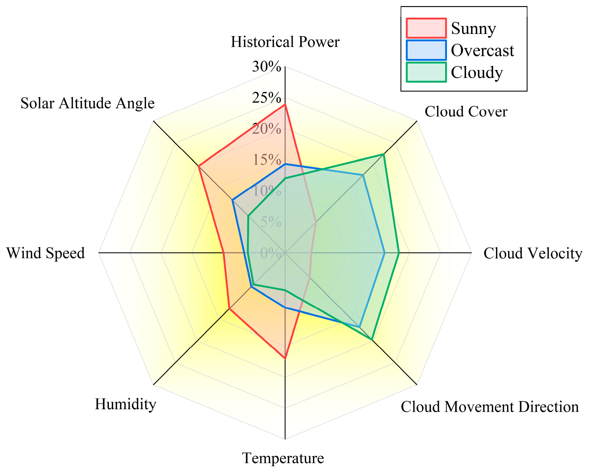
where d denotes the total number of input features. The resulting $C_j$ values were used to construct the radar charts in Figure 7. Daily-block permutation was adopted instead of pointwise random permutation to preserve the internal temporal structure of the 5-min time series. The analysis was conducted separately for the sunny, cloudy, and overcast test subsets.

As shown in Figure 7, the radar charts for the three weather types exhibit clearly different shapes, indicating that the dominant features in photovoltaic power forecasting vary dynamically with meteorological conditions. Under sunny conditions, historical power and solar altitude angle make the largest contributions, whereas cloud-image-related features have relatively low importance. Under cloudy conditions, cloud-image features become dominant in the forecasting process, with cloud motion reaching its highest importance, while the contribution of conventional meteorological factors decreases. Under overcast conditions, cloud coverage becomes the most important feature.

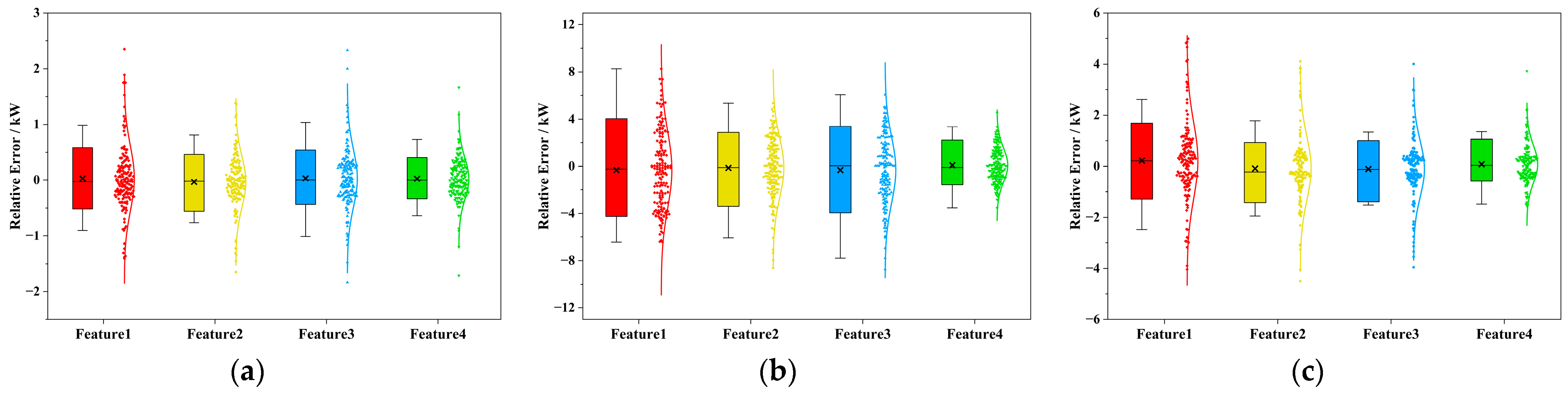
To more accurately evaluate the forecasting performance under different conditions, the error distributions between the predicted and actual values are shown in Figure 8. Feature 4 exhibits a more concentrated error distribution across all three weather conditions, with a smaller box range and lower dispersion than the other feature combinations. This indicates that fusing static and dynamic cloud-image features not only reduces the overall prediction error but also improves the stability of the forecasting results. In particular, under cloudy conditions, the error distribution of Feature 1 is relatively dispersed, whereas the error range of Feature 4 is significantly narrowed. This suggests that cloud-image feature fusion can effectively enhance the model’s adaptability to complex cloud variations and abrupt photovoltaic power fluctuations. Overall, as shown in Figure 7 and Figure 8, integrating meteorological data, static cloud-image features, and dynamic cloud-image features as model inputs enables better performance in fitting power variation trends, tracking local fluctuations, and stabilizing prediction errors, thereby further validating the effectiveness of the proposed static–dynamic cloud-image feature fusion method.

The forecasting errors under cloudy conditions are shown in

Table 3. Evaluation metrics for prediction results based on different features under cloudy weather conditions.

Feature	RMSE/kW	MAE/kW	nMAE/%	R2/%
feature 1	3.266	2.669	8.87	74.61
feature 2	2.555	1.984	6.59	81.42
feature 3	1.882	1.468	4.88	85.58
feature 4	1.436	1.152	3.83	90.95

. Photovoltaic power is strongly affected by cloud shading and motion, and the model produces larger forecasting errors overall than under sunny and overcast conditions. Compared with Feature 1, both Feature 2 and Feature 3 effectively reduce the prediction errors, indicating that cloud-image features provide information on sky conditions that is difficult to represent using conventional meteorological data alone. Compared with Feature 2, Feature 3 achieves lower RMSE and MAE, suggesting that under cloudy conditions, dynamic features such as cloud motion speed and direction can more effectively reflect the influence of cloud-shading variations on photovoltaic power over short timescales. When static and dynamic features are introduced simultaneously, Feature 4 achieves the best results, with RMSE and MAE reduced to 1.436 kW and 1.152 kW, respectively, and R² increased to 90.95%. Compared with Feature 1, Feature 4 reduces RMSE and MAE by 56.03% and 56.84%, respectively, while improving R² by 16.34%. These results indicate that fusing static and dynamic cloud-image features can significantly enhance the forecasting capability of the model under complex and highly variable weather conditions.

The forecasting errors under overcast conditions are shown in

Table 4. Evaluation metrics for prediction results based on different features under overcast weather conditions.

Feature	RMSE/kW	MAE/kW	nMAE/%	R2/%
feature 1	1.514	1.051	3.49	91.57
feature 2	1.237	0.821	2.73	94.13
feature 3	1.344	0.967	3.21	93.42
feature 4	0.836	0.633	2.10	97.82

, where Feature 4 again achieves the best forecasting performance. Compared with Feature 1, Feature 4 reduces RMSE and MAE by 44.78% and 39.77%, respectively, while increasing R² by 6.25%. A comparison between Feature 2 and Feature 3 shows that static cloud-image features provide a slightly greater improvement than dynamic cloud-image features. This may be because cloud cover is relatively continuous under overcast conditions, and the influence of overall cloud motion on short-term power variations is less direct than that of the cloud-cover state. Therefore, static features such as cloud coverage can more effectively characterize irradiance variations under this type of weather.

Overall, the results under the three weather conditions show that introducing either static or dynamic cloud-image features alone can improve the forecasting performance of CNN-Autoformer to varying degrees, but their effects vary significantly across weather conditions. Under sunny and overcast conditions, static cloud-image features contribute more noticeably to improving the prediction results. Under cloudy conditions, dynamic features such as cloud motion speed and direction are more effective in characterizing photovoltaic power fluctuations. After static and dynamic features are fused, the model achieves the lowest RMSE, the lowest MAE, the lowest nMAE and the highest R² under all three weather conditions, demonstrating the effectiveness and advantages of the proposed static–dynamic cloud-image feature fusion method for ultra-short-term photovoltaic power forecasting.

4. Conclusions

In ultra-short-term photovoltaic power forecasting, cloud-induced shading of solar irradiance and the short-term evolution of cloud cover are key factors that cause rapid fluctuations in photovoltaic power. Conventional meteorological data are often insufficient to fully characterize cloud-shading conditions and cloud-motion trends. To address this limitation, this study focuses on ground-based cloud image processing, static–dynamic cloud-image feature extraction, and deep learning-based forecasting model construction. An ultra-short-term photovoltaic power forecasting method integrating multidimensional ground-based cloud-image features with CNN-Autoformer is proposed. Model comparison experiments and input-feature combination experiments under different weather conditions demonstrate the effectiveness of the proposed model architecture and cloud-image feature fusion method. The main conclusions are as follows.

(1)

A comprehensive workflow for ground-based cloud image processing and feature extraction is developed. To address fisheye distortion, illumination variation, and solar interference in raw ground-based cloud images, image correction, image enhancement, and solar-interference suppression are applied to improve image quality. Based on the processed images, static features such as cloud coverage are extracted using threshold segmentation, while dynamic features such as cloud motion speed and motion direction are obtained using an optical flow method. This workflow characterizes the influence of clouds on photovoltaic output from two perspectives: the current cloud-shading condition and the short-term evolution trend of cloud motion. As a result, it provides the forecasting model with input information that is more physically interpretable and more representative in both temporal and spatial dimensions.

(2)

A hybrid CNN-Autoformer forecasting model is proposed. The model first employs a CNN to extract local short-term variation information from photovoltaic power, meteorological data, and cloud-image features. It then uses the sequence decomposition architecture and autocorrelation mechanism of Autoformer to capture trend components, periodic components, and long-term dependencies in the power sequence. In this way, local feature extraction and global temporal modeling are effectively integrated. Compared with CNN, Transformer, Autoformer, and CNN-Transformer, the proposed CNN-Autoformer achieves better forecasting performance under sunny, cloudy, and overcast conditions. The experimental results show that the proposed model achieves better forecasting accuracy than the selected learning-based baselines under the three evaluated weather conditions.

(3)

By fixing CNN-Autoformer as the forecasting model and constructing different input feature combinations, the contributions of static and dynamic cloud-image features to forecasting performance are further verified. The results show that under sunny and overcast conditions, photovoltaic power variations are relatively smooth or cloud cover is relatively continuous. Therefore, static features such as cloud coverage contribute more significantly to improving prediction accuracy. Under cloudy conditions, cloud shading and motion occur more frequently, and photovoltaic power exhibits stronger non-stationarity and abrupt variations. In this case, dynamic features such as cloud motion speed and motion direction play a more important role in improving prediction accuracy. By fusing static and dynamic cloud-image features, the model can simultaneously characterize the current cloud-shading condition and the future evolution trend of cloud motion, thereby achieving higher forecasting accuracy and stability under different weather conditions.

Overall, the proposed ultra-short-term photovoltaic power forecasting framework based on the fusion of static and dynamic ground-based sky-image features and CNN–Autoformer achieved improved forecasting accuracy relative to the selected learning-based comparison models under sunny, cloudy, and overcast conditions. In particular, the incorporation of cloud-image features improved the model’s ability to characterize rapid power fluctuations caused by cloud shading and motion. However, these conclusions are limited to the evaluated Stanford University site and the selected study period. Therefore, the present results demonstrate the effectiveness of the proposed method under the specified experimental conditions. The transferability of the proposed framework may be affected by several site-dependent factors. Different geographical locations and seasons may exhibit distinct solar geometries, cloud climatology, irradiance distributions, and photovoltaic power patterns. In addition, variations in camera orientation, fisheye projection, image resolution, exposure characteristics, and color response may alter the distributions of the extracted cloud-coverage and cloud-motion features. Consequently, application to a new site may require site-specific camera calibration, solar-position mapping, feature normalization, and model fine-tuning or retraining.

Future work will, therefore, extend the evaluation to full-year datasets and multiple sites with different climatic conditions, camera configurations, and photovoltaic technologies. Cross-site transfer learning and domain-adaptation methods will also be investigated to reduce the amount of site-specific training data required. In addition, uncertainty forecasting will be incorporated to further improve the practical applicability of the proposed method in photovoltaic dispatch and operational control.

References

1. Dhabi, A. International Renewable Capacity Statistics 2026; International Renewable Energy Agency: Abu Dhabi, United Arab Emirates, 2026. [Google Scholar]
2. Zhen, H.; Niu, D.; Wang, K. Photovoltaic Power Forecasting Based on GA Improved Bi-LSTM in Microgrid Without Meteorological Information. Energy 2021, 231, 120908. [Google Scholar] [CrossRef] [Scilit]
3. Limouni, T.; Yaagoubi, R.; Bouziane, K. Accurate One Step and Multistep Forecasting of Very Short-Term PV Power Using LSTM-TCN Model. Renew. Energy 2023, 205, 1010–1024. [Google Scholar] [CrossRef] [Scilit]
4. Das, O.; Dahlioui, D.; Zafar, H.M. Ultra-Short Term PV Power Forecasting Under Diverse Environmental Conditions: A case study of Norway. Energy Convers. Manag. X 2025, 27, 101072. [Google Scholar] [CrossRef] [Scilit]
5. Gong, J.; Qu, Z.; Zhu, Z. Parallel TimesNet-BiLSTM Model for Ultra-Short-Term Photovoltaic Power Forecasting Using STL Decomposition and Auto-Tuning. Energy 2025, 320, 135286. [Google Scholar] [CrossRef] [Scilit]
6. Prashant, M.; Rahul, C.; Shyam, S.C. A Power Prediction Model and Its Validation for A Roof Top Photovoltaic Power Plant Considering Module Degradation. Sol. Energy 2021, 224, 184–194. [Google Scholar] [CrossRef] [Scilit]
7. Dong, Y.; Zhang, H.; Wang, C. A Novel Hybrid Model Based on Bernstein Polynomial with Mixture of Gaussians for Wind Power Forecasting. Appl. Energy 2021, 286, 116545. [Google Scholar] [CrossRef] [Scilit]
8. Adar, M.; Babay, M.-A.; Boussif, M.; Khaouch, Z. Optimization of Photovoltaic System Modelling: A Comparative Study and Experimental Validation Using Bond Graph Methodology and a Genetic Algorithm. Adv. Transdiscipl. Eng. 2024, 61, 723–730. [Google Scholar] [CrossRef] [Scilit]
9. Connor, S.; Mominul, A.; Alhussein, A. Machine Learning for Forecasting a Photovoltaic (PV) Generation System. Energy 2023, 278, 127807. [Google Scholar] [CrossRef] [Scilit]
10. Jung, Y.; Jung, J.; Kim, B. Long Short-Term Memory Recurrent Neural Network for Modeling Temporal Patterns in Long-Term Power Forecasting for Solar PV Facilities: Case Study of South Korea. J. Clean. Prod. 2019, 250, 119476. [Google Scholar] [CrossRef] [Scilit]
11. Adar, M.; Babay, M.-A.; Touairi, S. Experimental Validation of Different PV Power Prediction Models under Beni Mellal Climate. Energy Nexus 2022, 5, 100050. [Google Scholar] [CrossRef] [Scilit]
12. Mohamad, H.A.; Bukhari, S.M.S.; Hamza, M.Z.; Mansoor, M.; Chen, W. COA-CNN-LSTM: Coati Optimization Algorithm-Based Hybrid Deep Learning Model for PV/Wind Power Forecasting in Smart Grid Applications. Appl. Energy 2023, 349, 121638. [Google Scholar] [CrossRef] [Scilit]
13. Deniz, K. SolarNet: A Hybrid Reliable Model Based on Convolutional Neural Network and Variational Mode Decomposition for Hourly Photovoltaic Power Forecasting. Appl. Energy 2021, 300, 117410. [Google Scholar] [CrossRef] [Scilit]
14. Shi, C.; Su, Z.; Zhang, K. CloudSwinNet: A Hybrid CNN-Transformer Framework for Ground-Based Cloud Images Fine-Grained Segmentation. Energy 2024, 309, 133128. [Google Scholar] [CrossRef] [Scilit]
15. Chen, J.; Peng, T.; Qian, S. An Error-Corrected Deep Autoformer Model Via Bayesian Optimization Algorithm and Secondary Decomposition for Photovoltaic Power Prediction. Appl. Energy 2025, 377, 124738. [Google Scholar] [CrossRef] [Scilit]
16. Demil, G.; Haghighi, T.A.; Klöve, B. Seeing Through the Clouds: Enhanced Snow And Cloud Segmentation in Sentinel-2 Imagery with mDeepLabV3+. Earth Sci. Inform. 2025, 18, 477. [Google Scholar] [CrossRef] [Scilit]
17. Mihulet, E.; Czibula, G.; Alexandrescu, S. Using Deep Learning for Enhancing the Performance of Ground-Based Cloud Images Classification. Stud. Inform. Control. 2025, 34. [Google Scholar] [CrossRef] [Scilit]
18. Wu, X.; Zhen, Z.; Zhang, J. Multidimensional Feature Extraction Based Minutely Solar Irradiance Forecasting Method Using All-Sky Images. IEEE Trans. Ind. Appl. 2024, 60, 4494–4504. [Google Scholar] [CrossRef] [Scilit]
19. Chen, Y.; Chen, J.; Huang, W. 3D Cumulus Cloud Scene Modelling and Shadow Analysis Method Based on Ground-Based Sky Images. Int. J. Appl. Earth Obs. Geoinf. 2022, 109, 102765. [Google Scholar] [CrossRef] [Scilit]
20. Liu, S.; Zhang, J.; Zhang, Z. Integration Transformer for Ground-Based Cloud Image Segmentation. IEEE Trans. Geosci. Remote Sens. 2023, 61, 5606712. [Google Scholar] [CrossRef] [Scilit]
21. Wang, Y.; Wang, X.; Hao, D. Combined Ultra-Short-Term Prediction Method of PV Power Considering Ground-Based Cloud Images and Chaotic Characteristics. Sol. Energy 2024, 274, 112597. [Google Scholar] [CrossRef] [Scilit]
22. Kevin, B.; Robin, G.; Guillaume, B. A Generic Methodology to Efficiently Integrate Weather Information in Short-Term Photovoltaic Generation Forecasting Models. Sol. Energy 2022, 244, 401–413. [Google Scholar] [CrossRef] [Scilit]
23. Li, X.; Lu, Z.; Zhou, Q.; Xu, Z. A Cloud Detection Algorithm with Reduction of Sunlight Interference in Ground-Based Sky Images. Atmosphere 2019, 10, 640. [Google Scholar] [CrossRef] [Scilit]
24. Nie, Y.; Li, X.; Scott, A. SKIPP’D: A SKy Images and Photovoltaic Power Generation Dataset for Short-Term Solar Forecasting. Sol. Energy 2023, 255, 171–179. [Google Scholar] [CrossRef] [Scilit]
Figure 1. Steps of the latitude and longitude correction algorithm.
Energies 19 03978 g001
Figure 2. Cloud identification results based on the Otsu method.
Energies 19 03978 g002
Figure 3. RAFT network architecture.
Energies 19 03978 g003
Figure 4. Tracking results of cloud motion.
Energies 19 03978 g004
Figure 5. Architecture of the CNN-Autoformer model.
Energies 19 03978 g005
Figure 6. Comparison of CNN-Autoformer prediction results under different combinations of input features: (a) Prediction curve under sunny conditions; (b) Prediction curve under cloudy conditions; (c) Prediction curve under overcast conditions.
Energies 19 03978 g006
Figure 7. Feature importance analysis.
Energies 19 03978 g007
Figure 8. Prediction error distribution of CNN-Autoformer with different input feature combinations: (a) Distribution of prediction errors under sunny conditions; (b) Distribution of prediction errors under cloudy conditions; (c) Distribution of prediction errors under overcast conditions.
Energies 19 03978 g008