An Innovative Method for Modeling Inertia in Wind Turbine Emulators: Concept, Implementation, and Laboratory Testing

Abstract

This monograph synthesizes the current state of knowledge on mathematical models and wind turbine (WT) modeling methods, in particular in the field of implementation of wind turbine emulators (WTE). The areas covered include the methods used to create a physical and simulation model of a WT and its individual components, as well as an analysis of published results of research conducted using WTEs. The analysis of wind turbine generator inertia modeling and its impact on accurate simulation of WT operation in dynamic states is given special attention in this publication. This publication provides in-depth analysis of the dynamic properties of WTEs. The analysis identifies the shortcomings and limitations of existing models. As a result of the research, an original and effective method was proposed for creating an emulator of a real WT with a doubly fed induction machine. Achieving significantly better simulation accuracy in dynamic states than in models found in scientific publications. The tests results presented in the paper proved that the dynamic properties of the emulator developed by the authors allow its use in research and development work in a laboratory on a real turbine. The proposed solution was used to develop a scalable emulator of a real WT utilizing the physical properties of a doubly fed machine which is an element of the emulator.

1. Introduction

The suitability of a Wind Turbine Emulator for dynamic investigations depends on its ability to reproduce not only the steady-state operating point of the modeled wind turbine, but also its response to disturbances. Such a response is governed by the control structure and parameters, as well as by the kinetic energy stored in the rotating components of the drive train. Whereas the control algorithms can be reconfigured in both the modeled WT and the WTE, the physical inertia of the laboratory motor–generator set (MG set) is determined by the machines installed in the test bench and generally differs from that of a full-scale turbine. Consequently, accurate emulation requires a method that adjusts the equivalent inertial response of the WTE without replacing or mechanically modifying its rotating components. The scalable wind turbine emulators (SWTE) architecture that motivated this study was introduced in [1].

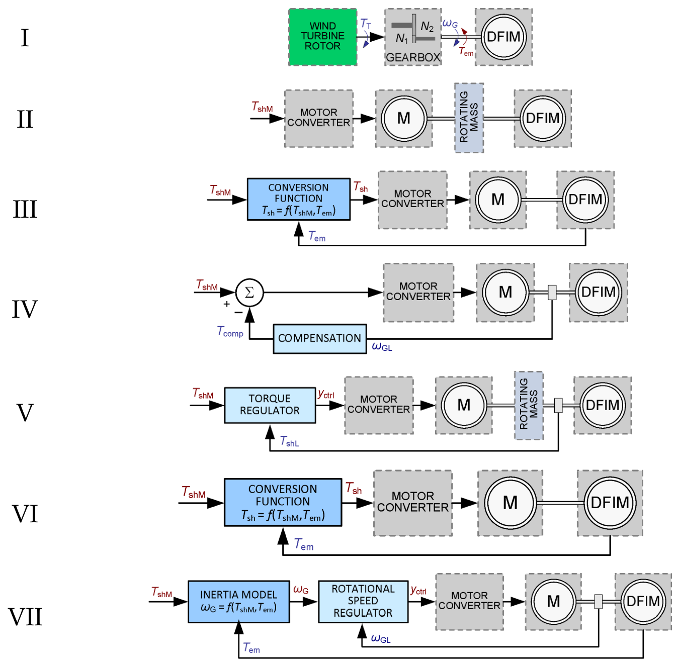
Figure 1 presents schematic diagrams of the drive trains of the modeled WT (I) and the WTE with a doubly fed induction machine (DFIM) in the WT inertia modeling variants (II–VII) considered in the literature and the two concepts developed by the authors. Concepts for modeling WT inertia can be grouped according to their operating principle.

Table 1. Summary of Potential Solutions to the Problem of Inertia Emulation in WTE—Authors’ Synthesis.

	Method	Controller	Requirements	Disadvantages
II	Additional rotating mass	Open-loop shaft torque control	Knowledge of induction motor loss characteristics	- Necessity to mount a large rotating mass on the shaft (i), - Inconvenient scalability (ii), - Difficulty in compensating for motor losses.
III	Scaling function			- Difficulty in compensating for motor losses, - Limited range of modeled compensation inertia $T_{comp}=f\left({\displaystyle \frac{d\omega }{dt}},\omega \right)$ and sensitivity of the ${\displaystyle \frac{d\omega }{dt}}$ coupling to disturbances.
IV	Compensation function	Open-loop compensation signal	Encoder	- Limited range of modeled inertia, - The coupling from the velocity derivative is sensitive to disturbances.
V	Additional rotating mass	Shaft torque regulator	Torque meter	- Necessity to mount a large rotating mass on the shaft (i), - Inconvenient scalability (i)(ii), - Absence of a torque meter (iii), - Reduced torque wrench accuracy in dynamic states.
VI	Scaling function			- Absence of a torque meter (ii), - Reduced torque wrench accuracy in dynamic states.
VII	Inertia model	Shaft speed regulator	Encoder	- Implementation requires reprogramming of converter controllers, which requires the involvement of the manufacturer.

⁽ⁱ⁾ High mass and size of the flywheel compared to the DFIM rotor. ⁽ⁱⁱ⁾ Scaling of the constant inertia requires ready-made flywheel components and assembly activities related to changing them. ⁽ⁱⁱⁱ⁾ Applies to the implementation of a SWTE in the LINTE^2 laboratory.

presents a summary of solutions for adapting the WTE MG set to emulate the dynamic properties of a high-power wind turbine generator.

In this publication, the WTE implementations described in the literature and two original concepts of an improved version of the WTE (VI, VII) are discussed, which allow the WTE to be used for research in dynamic states of changes in operating conditions. Laboratory tests of inertia modeling according to concept VII were performed and are discussed. The tests were performed with the use of a Scalable Wind Turbine Emulator (SWTE), which was implemented as a test bench at the Laboratory of Innovative Electrical Power Technologies and Renewable Energy Sources Integration LINTE^2 at Gdańsk University of Technology.

The main aspect determining the dynamic properties of the WTE is the inertia of the rotating elements of the MG set. In the literature on the subject, four approaches to inertia modeling can be distinguished:

• Modeling of a real turbine using a generator in the WTE with similar power to the one in the WT. In ref. [2], a generator with the same power was used to model a small 11 kW WT. This method gives very good results while the time constant of the WT generator rotor is similar to the equivalent time constant of the rotating elements of the WTE MG set.
• Omission of inertia without a comparative analysis of the dynamic properties of the MWT and its corresponding WTE [3,4,5,6,7,8,9,10]. This is the simplest and most common approach, although it limits the use of the WTE to static or quasi-static emulation.
• Compensation of the inertia of the WTE MG set rotors by installing additional rotating mass on the WTE MG shaft [11]. This method allows for very accurate modeling of the inertia of the WT generator rotor, with the drive train modeled in a very simplified manner (the difference between the losses in the MG set motor and the losses in the WT drive train is ignored).
• Compensation of the inertia of WTE MG set rotors through appropriately modified MG set motor control [12,13,14,15,16,17]. The modification may consist of rescaling the drive torque in the WT mechanical part model or its compensation with $T_{comp}=f\left({\displaystyle \frac{\mathrm{d}\omega }{\mathrm{d}t}},\omega \right)$. The first method does not take into account losses in the MG set motor, while the second has a limited range of modeled inertia, and the coupling from the velocity derivative is sensitive to disturbances.

In several recent configurations of Wind Turbine Emulators (WTEs), inertia modeling is based on previously published compensation techniques [18,19,20]. However, in most cases, the challenge of accurately replicating turbine inertia within WTE systems remains unaddressed [21,22,23,24,25,26,27,28]. The focus of these studies tends to be on control strategies for the motor-side converter, while simulation models typically incorporate simplified representations of the turbine rotor, the Maximum Power Point Tracking (MPPT) module, and the power controller.

The effect of correct modeling of the dynamic properties of a WT is a good representation of the angular speed ω_MG of the simulated WT generator with the speed of the WTE generator ω_LG. To achieve this, it is necessary to use a two-mass turbine shaft model. This approach was implemented in the SWTE used in the study, the results of which are presented in [1].

In the WTE described in the literature, a single-mass model with various modifications is commonly used:

• without compensation [5,8,13],
• with simple inertia correction [12,29],
• with compensation based on generator rotor speed [14,30],
• with compensation based on the velocity derivative [15,16,17,31,32].

High-power WT emulation using a single-mass model does not take into account torsional oscillations on the shaft between the generator rotor and the turbine rotor. Modeling the dynamic properties of a high-power WT requires emulation of the inertia of the rotating elements of the MWT (turbine and generator rotors) while taking into account the inertia of the rotating elements of the WTE MG set (motor and generator rotors). The moments of inertia of other rotating components of the WT, such as turbine and generator shafts and gear wheels, are negligible compared to the moments of inertia of the turbine rotor and generator rotor and therefore have been omitted in further considerations.

The inertia of the rotating components is determined by the moment of inertia J, expressed in absolute units $\left[\mathrm{k}\mathrm{g}·{\mathrm{m}}^2\right]$. It is more convenient to parameterize the model using relative units. Therefore, the inertia constant H expressed in seconds is used. The relationship between the quantities is described by (1).

$$H=J·{\displaystyle \frac{{{\omega }_{\mathrm{s}}}^2}{2·S_{\mathrm{n}}}}$$

(1)

The inertia constant of the H_GM (Index: G—refers to the parameters of the generator, M—modeled turbine) high-power WT generator is greater than the equivalent inertia constant of the generator and motor rotors of the WTE MG set (H_GM > H_L, index: L—refers to the parameters of the laboratory WTE MG set, ML/GL—motor/generator of MG set). Furthermore, the inertia constant of the H_TM (Index: T—refers to the turbine) wind turbine rotor is significantly greater than the equivalent inertia constant of the MG set rotors (H_GM >> H_L). It should therefore be expected that when using a low-power MG set to model a high-power WT, there will be a problem with adequately reproducing the dynamic properties.

This article will present the modeling methods described in the literature and used in WTEs based on the modification of the drive torque signal T, as well as the author’s control concepts shown in Figure 1:

• scaling function with torque controller (VI),
• application of inertia model and speed controller (VII).

Furthermore, it was demonstrated that appropriate control of the angular speed of the generator rotor of the WTE allowed for correct modeling of the turbine properties in dynamic states with sufficient accuracy to enable the use of the WTE for reliable laboratory testing. In refs. [15,16] this operation is often referred to as inertia compensation or emulation.

2. Compensation of Inertia by Modifying Torque Signal Control

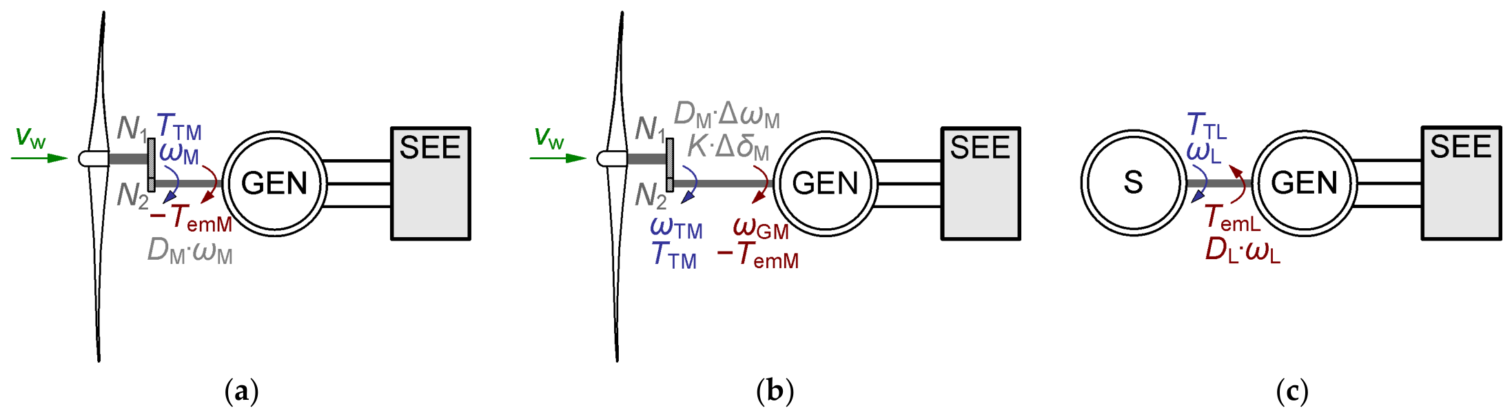
This concept is based on the assumption that it is possible to model the inertia of a high-power WT generator using a low-power machine set by appropriately controlling the drive motor. Considerations regarding feasibility should begin with an analysis of the system of two rotating masses, namely the turbine rotor and the generator rotor (Figure 2).

Assuming for simplicity, the connection of the turbine and the generator rotors is rigid and the rotors rotate synchronously (Figure 2a). This assumption is often made in the methods described in scientific literature. Then, according to the second law of rotational motion of a rigid body, they are described by the equation of motion (2):

$$J·{\displaystyle \frac{\mathrm{d}\omega }{\mathrm{d}t}}=T_{\mathrm{T}}-T_{\mathrm{e}\mathrm{m}}-D·\omega$$

(2)

where

$$J=J_{\mathrm{T}}+J_{\mathrm{G}}$$

(3)

Equation (2) for the single-mass modeled WT (Figure 2a) and for the WTE MG set (Figure 2c) will take the form of a system of (4) (Index: G—refers to the parameters of the generator, T—turbine, M—modeled turbine, L—laboratory WTE MG set, ML/GL—motor/generator of MG set):

$$\left.\begin{array}{c}{J}_{\mathrm{M}}{\displaystyle \frac{\mathrm{d}{\omega }_{\mathrm{M}}}{\mathrm{d}t}}=T_{\mathrm{T}\mathrm{M}}-T_{\mathrm{e}\mathrm{m}\mathrm{M}}-D_{\mathrm{M}}{\omega }_{\mathrm{M}}\\ J_{\mathrm{L}}{\displaystyle \frac{\mathrm{d}{\omega }_{\mathrm{L}}}{\mathrm{d}t}}=T_{\mathrm{T}\mathrm{L}}-T_{\mathrm{e}\mathrm{m}\mathrm{L}}-D_{\mathrm{L}}{\omega }_{\mathrm{L}}\end{array}\right\}$$

(4)

where

$$\left.\begin{array}{c}{J}_{\mathrm{M}}={\left({\displaystyle \frac{N_1}{N_2}}\right)}^2·J_{\mathrm{T}\mathrm{M}}+J_{\mathrm{G}\mathrm{M}}\\ J_{\mathrm{L}}=J_{\mathrm{M}\mathrm{L}}+J_{\mathrm{G}\mathrm{L}}\end{array}\right\}$$

(5)

The two-mass model in a system with a gear, connected by two shafts, each with its own stiffness and damping (Figure 2b), can be reduced to a system with a single shaft of equivalent stiffness and damping without a gear [33], then the equation of motion (4) takes the form (6) (Index: 1—refers to the value on the shaft before the gearbox, on the turbine rotor side, at the end of the shaft on the rotor side. Please note that with this notation, the driving torque transferred through the gearbox to the generator side $T_{\mathrm{T}}=T_{\mathrm{s}\mathrm{h}}$. Notation used interchangeably in the article).

$$\left.\begin{array}{c}{J}_{\mathrm{T}\mathrm{M}}{\displaystyle \frac{\mathrm{d}{\omega }_{\mathrm{T}\mathrm{M}}}{\mathrm{d}t}}=T_{\mathrm{T}\mathrm{M}}-D_{\mathrm{M}}{∆\omega }_{\mathrm{M}}-K·∆{\delta }_{\mathrm{M}}\\ J_{\mathrm{G}\mathrm{M}}{\displaystyle \frac{\mathrm{d}{\omega }_{\mathrm{G}\mathrm{M}}}{\mathrm{d}t}}=-T_{\mathrm{e}\mathrm{m}\mathrm{M}}-D_{\mathrm{M}}{∆\omega }_{\mathrm{M}}+K·∆{\delta }_{\mathrm{M}}\end{array}\right\}$$

(6)

where

$$\left.\begin{array}{c}\begin{array}{c}{∆\omega }_{\mathrm{M}}={\omega }_{\mathrm{T}\mathrm{M}}-{\omega }_{\mathrm{G}\mathrm{M}}\\ ∆{\delta }_{\mathrm{M}}={\delta }_{\mathrm{T}\mathrm{M}}-{\delta }_{\mathrm{G}\mathrm{M}}\\ J_{\mathrm{T}}={\left({\displaystyle \frac{N_2}{N_1}}\right)}^2·J_{\mathrm{T}1}\end{array}\\ \begin{array}{c}{T}_{\mathrm{T}}={\displaystyle \frac{N_2}{N_1}}·T_{\mathrm{T}1}\\ {\omega }_{\mathrm{T}}={\displaystyle \frac{N_2}{N_1}}·{\omega }_{\mathrm{T}1}\\ {\delta }_{\mathrm{T}}={\displaystyle \frac{N_2}{N_1}}·{\delta }_{\mathrm{T}1}\end{array}\end{array}\right\}$$

(7)

Most publications assume that the mechanical model of a WT, as implemented in the simulation component of WTE, determines the mechanical T_TL torque on the shaft of the MG set. In refs. [13,30], the torque on the machine shaft was regulated using torque measurement. The T_TL torque can also be determined using an estimator, which, according to the authors of [14], also allows for early detection of torque increases after a sudden change in wind, which can be appropriately used in the control system.

The equality of the angular velocity and angular acceleration of the WT generator rotor and the WTE generator rotor, expressed in relative units, is the basic criterion for the quality of the modeling of the dynamic properties of the WTE, and thus the quality of the WTE. For the two-mass model of WT and assuming a rigid shaft of the WTE MG set, since the equality of the generator rotor speeds is crucial, the condition takes the form (8).

$$\left.\begin{array}{c}{\omega }_{\mathrm{L}}={\omega }_{\mathrm{G}\mathrm{M}}\\ {\displaystyle \frac{\mathrm{d}{\omega }_{\mathrm{L}}}{\mathrm{d}t}}={\displaystyle \frac{\mathrm{d}{\omega }_{\mathrm{G}\mathrm{M}}}{\mathrm{d}t}}\end{array}\right\}$$

(8)

For the single-mass model, the condition remains valid, because then ${\omega }_{\mathrm{G}\mathrm{M}}={\omega }_{\mathrm{T}\mathrm{M}}={\omega }_{\mathrm{M}}$.

The fulfillment of the angular acceleration equality condition is the most commonly accepted criterion for the correct operation of a WT [12,13,14,15,16,17,30]. This is usually accompanied by the tacit assumption that the angular acceleration equality condition implies that angular velocities are equal. In most publications, the resistance torque is neglected, and the moment of inertia of the generator in the modeled turbine is assumed to be equal to that of the generator in the WTE. The first assumption does not introduce a significant simulation error. The second assumption, in the case where the inertia constant of the generator of the modeled WT differs from the equivalent inertia constant of the WTE MG set ($H_{\mathrm{G}\mathrm{M}}\ne H_{\mathrm{L}}$), leads to different disturbance transient responses of angular velocity and active power.

The consequences of an incorrect representation of generator inertia were previously investigated using the same validation model in [1]. Figure 12 in that study compares the transient responses of the reference wind farm model and the SWTE model under a short-circuit disturbance in the 110 kV grid and following a step change in the mechanical torque. When identical inertia constants were assigned to both models, the generator angular velocity responses remained closely aligned. The remaining differences, observed mainly in electromagnetic torque and active power, were associated with differences in the electrical parameters of the compared models.

A different response was obtained when the inertia constant of the SWTE model was reduced from H_M = 0.96 s to H_L = 0.56 s (H_M = 0.96 s—inertia constant of the rotor of DFIM of GE 1.5 wind turbine; H_L = 0.56 s—equivalent inertia constant of the rotors of the Laboratory MG set), while the remaining generator parameters were kept unchanged. In this case, a distinct separation of the angular velocity trajectories occurred during the transient state, and the relative rates of change in angular velocity reflected the ratio of the assigned inertia constants. The results presented in [1] therefore demonstrate that satisfactory representation of the electrical subsystem alone does not ensure adequate reproduction of WT dynamics. An incorrect inertia constant directly affects the generator-speed response and consequently reduces the fidelity of the WTE during disturbances.

These earlier observations provide the motivation for the comparative assessment performed in the present study. The transient responses obtained using the investigated inertia-modeling methods, together with the corresponding error estimates, are presented later in the article.

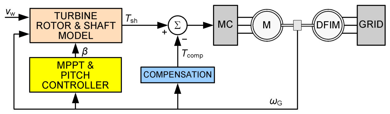
When controlling the WTE MG set with torque, in order to meet (8), the torque control signal must be compensated for accordingly. WTEs are constructed based on the assumption that the electromagnetic torques of the generators of the MWT and its emulator in relative units are equal ($T_{\mathrm{e}\mathrm{m}\mathrm{M}}=T_{\mathrm{e}\mathrm{m}\mathrm{L}}$). A schematic diagram of a WTE with motor converter (MC) control torque compensation is shown in Figure 3.

The authors of [32] propose correcting the signal $T_{\mathrm{L}}$ controlling the machine unit motor with a compensating signal:

$$T_{\mathrm{c}\mathrm{o}\mathrm{m}\mathrm{p}}=\left(J_{\mathrm{M}}-J_{\mathrm{L}}\right)·{\displaystyle \frac{\mathrm{d}\omega }{\mathrm{d}t}}+\left(D_{\mathrm{M}}-D_{\mathrm{L}}\right)·\omega$$

(9)

The kinetic friction component $\left(D_{\mathrm{M}}-D_{\mathrm{L}}\right)·\omega$ is negligible due to the low values: $D_{\mathrm{M}}, D_{\mathrm{L}}<0.01$. The coupling from the angular velocity derivative is of key importance in Equation (9). A block diagram of the algorithm for determining the compensating component T_comp with coupling from the angular velocity derivative, ignoring the kinetic friction component, given by Equation (10), is shown in Figure 4a:

$$T_{\mathrm{c}\mathrm{o}\mathrm{m}\mathrm{p}}=\left(J_{\mathrm{M}}-J_{\mathrm{L}}\right)·{\displaystyle \frac{\mathrm{d}\omega }{\mathrm{d}t}}$$

(10)

As a result of an analysis of the inertia compensation method (10) carried out in publication [16], the authors concluded that the disadvantage of the method consists of the tendency for the compensating torque to oscillate. The reason indicated was the delay of the angular acceleration observer. The condition for compensation stability given by the authors is that condition (11) must be met:

$$J_{\mathrm{M}}<2·J_{\mathrm{L}}$$

(11)

In ref. [15], the analysis of the inertia compensator was carried out using the model defined by Equation (10). Oscillations were observed in the compensating torque signal at frequencies significantly higher than would be expected from the mechanical properties of the turbine. The cause was identified as coupling from the velocity derivative, and in particular, the effect of a one-step delay in calculating the derivative. Instead of calculating the derivative from the last two samples, a solution was proposed that consisted of introducing a simple filter with a weighted moving average calculated from the last two samples and the previously determined value at the input of the angular velocity derivative calculation block, which suppresses measurement noise. The weighted average filter algorithm proposed in the publication is defined by (12):

$${\widehat{\omega }}_{\mathrm{G}}\left[n\right]={\alpha }_{\mathrm{d}}·{\widehat{\omega }}_{\mathrm{G}}\left[n-1\right]+{\left({1-\alpha }_{\mathrm{d}}\right)·\omega }_{\mathrm{G}}\left[n\right]$$

(12)

The authors show that compensation formulated in this way improves the accuracy of velocity emulation for the case where $J_{\mathrm{M}}>2·J_{\mathrm{L}}$, but its operation strongly depends on the weight coefficient in the filter, which should be experimentally selected and tested. The weight coefficient value recommended by the authors: ${\alpha }_{\mathrm{d}}\approx 0.9$. A block diagram of the compensation moment T_comp with coupling from the angular velocity derivative with a weighted average angular velocity filter is shown in Figure 4b. While the relatively simple formulas for the torque compensating component (Equations (8) and (12)) presented in the publications cited so far are based on velocity measurements, publications [14,17,30] use a formula that scales the value of the control torque on the shaft of the MG set of the WTE based on the torque values on the shaft of the MWT generator and the electromagnetic torque of the WTE generator. In ref. [17], the control torque of the MG set of the WTE was scaled according to formula (13). The equivalent torque of mechanical losses was taken into account as $T_{\mathrm{F}}$. As in ref. [29], the authors accepted the assumption without explanation $J_{\mathrm{G}\mathrm{M}}=J_{\mathrm{G}\mathrm{L}}=J_{\mathrm{G}}$:

$$T_{\mathrm{L}}={\displaystyle \frac{J_{\mathrm{S}\mathrm{L}}+J_{\mathrm{G}}}{{{\left(\frac{N_1}{N_2}\right)}^2·J}_{\mathrm{T}\mathrm{M}}+J_{\mathrm{G}}}}·T_{\mathrm{M}}+{\displaystyle \frac{{\left(\frac{N_1}{N_2}\right)}^2·J_{\mathrm{T}\mathrm{M}}-J_{\mathrm{S}\mathrm{L}}}{{{\left(\frac{N_1}{N_2}\right)}^2·J}_{\mathrm{T}\mathrm{M}}+J_{\mathrm{G}}}}·T_{\mathrm{e}\mathrm{m}}+T_{\mathrm{F}}$$

(13)

In the implementation described, a torque estimator was used to determine the angular acceleration of the rotor and the velocity observer, based on measurements from the shaft encoder and processed through a phase-locked loop. The results presented in [17] demonstrate that the method performs well when emulating turbines whose equivalent moment of inertia exceeds that of the MG set $J_{\mathrm{M}}>J_{\mathrm{L}}$. If this condition is not satisfied, a noticeable delay in the velocity waveforms is observed. The authors of [30] proposed their own version of the formula for scaling the motor control torque, described by (14).

$$T_{\mathrm{L}}={\displaystyle \frac{J_{\mathrm{S}\mathrm{L}}}{{\left(\frac{N_1}{N_2}\right)}^2·J_{\mathrm{T}\mathrm{M}}}}{·T}_{\mathrm{M}}+{\displaystyle \frac{{\left(\frac{N_1}{N_2}\right)}^2·J_{\mathrm{T}\mathrm{M}}-J_{\mathrm{S}\mathrm{L}}}{{\left(\frac{N_1}{N_2}\right)}^2·J_{\mathrm{T}\mathrm{M}}}}{·T}_{\mathrm{e}\mathrm{m}}$$

(14)

where

$$J_{\mathrm{G}}=J_{\mathrm{G}\mathrm{M}}=J_{\mathrm{G}\mathrm{L}}$$

An assumption was also made in the case of $J_{\mathrm{G}\mathrm{M}}=J_{\mathrm{G}\mathrm{L}}$. The authors did not provide a physical justification for the assumptions used to derive the formula.

In ref. [14], two models of turbine rotor inertia with torque signal control of the MG set were proposed. The tests showed that the accuracy of the angular velocity simulation methods can be estimated at approximately 8%. The analysis of the above-mentioned published methods of inertia compensation prompted the authors of this paper to develop their own, more accurate method of inertia scaling. In order to achieve the scalability of the WTE, the basic assumption of the authors’ method was to minimize simplifying assumptions.

All tests presented in this article were carried out with the use of the existing structure of the SWTE test bench of the Laboratory of Innovative Electrical Power Technologies and Renewable Energy Sources Integration LINTE^2 of the Faculty of Electrical and Control Engineering at Gdańsk University of Technology [1]. The experimental setup was based on the WG2 test bench of the LINTE^2 Laboratory. Its motor-generator set consists of a 75 kW squirrel-cage induction motor directly coupled to a 55 kW doubly fed induction machine. Separate power converters supply the drive motor and the DFIM rotor circuit. The wind turbine and inertia models are executed in Simulink Real-Time at a sampling frequency of 1 kHz, while the motor converter controller operates at 16 kHz and receives shaft-speed feedback from an absolute encoder. The main hardware parameters are summarized in

Table 2. Basic SWTE parameters.

Component	Parameter
Motor	Squirrel-cage induction motor, 75 kW, 1488 rpm
Generator	Doubly fed induction machine, 55 kW, 1457 rpm
Mechanical coupling	Direct shaft coupling
Real-time platform	Simulink Real-Time, sampling frequency 1 kHz
Motor converter controller	Sampling frequency 16 kHz
Speed measurement	Absolute encoder
Power-electronic interface	Separate converters for the drive motor and DFIM rotor

, and a detailed description of the SWTE architecture is provided in [1].

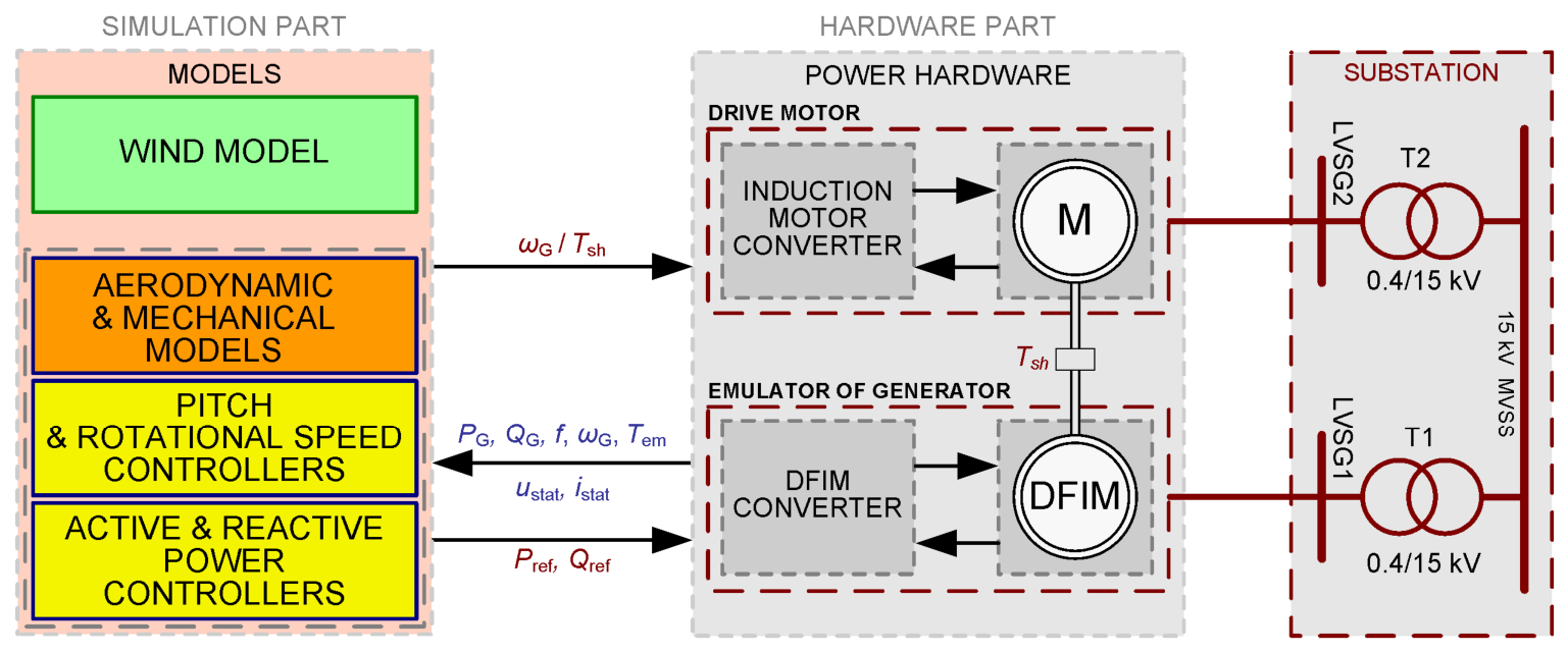
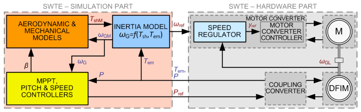
The general concept of the physical-digital model of a WT with an MG set is shown in Figure 5.

The WTE consists of a DFIM operating as a generator and a motor emulating a WT rotor driven by wind energy. The wind model and WT models (aerodynamic, mechanical, and control and regulation systems) are simulated in real time in the controller. The simulation part is coupled with measurement and control signals with the MG set. The quality criterion for the WTE system is the conformity of waveforms expressed in relative units of measurement between the WTE and the MWT, such as angular velocity, power, current, and voltage.

3. A Torque Computation Function Derived from Motion Equations and Parameterized by Inertia Constants

The first of the proposed original concepts involved applying a torque conversion function on the machine shaft, derived from physical relationships, to enable shaping the dynamic properties of the WTE system. This function, based on the current values of the mechanical torque of the modeled turbine and the electromagnetic torque of the WTE MG set generator, determines the mechanical torque that must be applied to the MG set shaft. The advantage of this approach is that the proposed function incorporates the derivative of speed, which is typically responsible for oscillatory transients and reduced accuracy. The application of the conversion function, as with any approach involving drive torque control at the generator shaft, necessitates a suitable control system. Modeling generator inertia with mechanical and electromagnetic torque scaling, using conversion functions derived from motion equations, accounts for the inertia constants of both the rotors of modeled WT and the MG set of the SWTE. In the case analyzed, the rotational motion of the turbine shaft, treated as a rigid body, is described by the following equation:

$$J·{\displaystyle \frac{\mathrm{d}\omega }{\mathrm{d}t}}=T_{\mathrm{s}\mathrm{h}}-T_{\mathrm{e}\mathrm{m}}$$

(15)

where $T_{\mathrm{s}\mathrm{h}}$—mechanical torque at the DFIM rotor shaft, $T_{\mathrm{e}\mathrm{m}}$—DFIM electromagnetic torque.

Equation (15) can be reduced to the following form:

$$T_{\mathrm{m}}·\omega ·{\displaystyle \frac{\mathrm{d}\omega }{\mathrm{d}t}}=P_{\mathrm{T}}-P_{\mathrm{e}}$$

(16)

By retaining angular velocity and its derivative on the left-hand side of the equation for the laboratory MG set (denoted by index L) and the modeled turbine assembly (denoted by index M), respectively, the equation can be expressed as follows:

$$\omega ·{\displaystyle \frac{\mathrm{d}\omega }{\mathrm{d}t}}={\displaystyle \frac{1}{T_{\mathrm{m}\mathrm{L}}}}·\left(P_{\mathrm{T}\mathrm{L}}-P_{\mathrm{e}\mathrm{L}}\right)$$

(17)

$$\omega ·{\displaystyle \frac{\mathrm{d}\omega }{\mathrm{d}t}}={\displaystyle \frac{1}{T_{\mathrm{m}\mathrm{M}}}}·\left(P_{\mathrm{T}\mathrm{M}}-P_{\mathrm{e}\mathrm{M}}\right)$$

(18)

Assuming that the SWTE exhibits, in relative units, the same angular velocity of the electric machine as the MWT—as well as the same electric power generated by the DFIMs—the left-hand sides of (17) and (18) are equal, and both equations can be written in the following form:

$$P_{\mathrm{T}\mathrm{L}}={\displaystyle \frac{T_{\mathrm{m}\mathrm{L}}}{T_{\mathrm{m}\mathrm{M}}}}{·P}_{\mathrm{T}\mathrm{M}}+\left(1-{\displaystyle \frac{T_{\mathrm{m}\mathrm{L}}}{T_{\mathrm{m}\mathrm{M}}}}\right)·P_{\mathrm{e}}$$

(19)

The torque conversion function at the shaft of the MG set in the SWTE takes the following form:

$$T_{\mathrm{T}\mathrm{L}}={\displaystyle \frac{T_{\mathrm{m}\mathrm{L}}}{T_{\mathrm{m}\mathrm{M}}}}·T_{\mathrm{T}\mathrm{M}}+\left(1-{\displaystyle \frac{T_{\mathrm{m}\mathrm{L}}}{T_{\mathrm{m}\mathrm{M}}}}\right)·T_{\mathrm{e}\mathrm{m}}$$

(20)

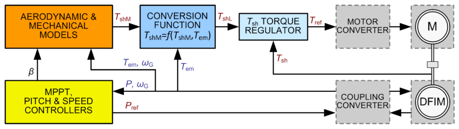
The conversion function (20) is used in Concept III—in the open-loop control configuration—and in Concept VI—in the torque control configuration (see Figure 1). The variables of the function $T_{\mathrm{T}\mathrm{L}}=f\left(T_{\mathrm{T}\mathrm{M}},T_{\mathrm{e}\mathrm{m}}\right)$ include the drive torque on the shaft of the generator in the MWT and the electromagnetic torque (i.e., the resistance torque of the SWTE generator), while the parameters comprise the inertia constants of the generators (20). To facilitate understanding of the relationships, the torque signal symbols T_TL and T_TjM are marked with indices T, L, and M, corresponding to the Turbine, generator of the Laboratory MG set, and generator of the Modeled WT, respectively. Neglecting losses in the converter and the motor, the drive torque at the rotor shaft DFIM T_sh is assumed to be equal to the reference torque T_ref controlling the converter. However, this solution does not provide satisfactory accuracy in emulating the rotational speed of the generator rotor, and its implementation was therefore rejected. Figure 6 presents a conceptual diagram of the original Concept VI (see Figure 1), which models inertia by applying the drive torque conversion function (20) together with a torque controller at the shaft of the SWTE MG set. Since the A&MM module implements a two-mass turbine shaft model and the conversion function scales the generator driving torque $T_{\mathrm{s}\mathrm{h}\mathrm{M}}$ modeled to the WTE MG set driving torque $T_{\mathrm{s}\mathrm{h}\mathrm{L}}$ with a rigid shaft, the WTE implements the two-mass nature of the WT.

In Concept VI, the controller regulates the torque at the generator shaft of the MG set via a converter supplying the asynchronous motor. Determining the rotor shaft torque T_sh from electrical signal measurements of the DFIM would result in a control structure highly sensitive to disturbances, leading to reduced accuracy and susceptibility to oscillations. This method requires the installation of a torque sensor on the shaft, which may pose mechanical and assembly challenges. Furthermore, even high-quality torque sensors fail to maintain nominal accuracy during transient states, which would directly affect the precision of rotor speed emulation in the WTE generator under dynamic conditions. The steady-state accuracy is approximately 0.5%. Response time errors are particularly significant in two-mass models, where the mutual torsional oscillations between rotating masses would be distorted.

4. Generator Inertia Model

The second proposed concept concerns the adjustment of the equivalent inertia constant of the MG set of the SWTE, incorporating inertia modeling within the torque control path and a speed controller (Method VII). The original concept is illustrated in Figure 7.

The SWTE drive transmission system is based on a two-mass model. Structurally, it consists of a simulated turbine rotor and shaft coupled to a real DFIM. The shaft torque signal—determined through simulation—drives the inertia model of the generator in the MWT. The shaft angular velocity ω_ref = ω_GM, simulated within the inertia model, works as the control signal for the converter supplying the asynchronous motor that drives the MG set. The inertia model of the rotor of the DFIM of the emulated WT used in this method is shown in Figure 8.

The inertia model and the rotational speed controller of the SWTE MG set can be implemented either in the simulation computer or within the converter controller supplying the asynchronous motor (M). The location of these components affects both the operational quality and the usability of the SWTE system. The advantages and disadvantages of different implementation configurations are summarized in

Table 3. System Configuration Analysis: Generator Rotor Inertia Model—Speed Controller in the implementation of Method VII for Inertia Emulation in WTE—Original Conceptual Synthesis.

Module Location		Advantages	Disadvantages
Inertia Model	Speed Controller
SLRT	SLRT	- possibility of structural and parametric reconfiguration during run-time; - real-time access to signals and parameters	- disturbances in transmitted electromagnetic torque and rotational speed signals—to ensure signal integrity, filtering is required (recommended filter time constant: 10 ms ≤ T ≤ 20 ms)
SLRT	MCC	Inertia model: - possibility of structural and parametric reconfiguration during run-time; - real-time access to signals and parameters; Speed controller: - sampling frequency (fp = 16 kHz), - undisturbed measurement of rotational speed and electromagnetic torque	Inertia model: - disturbances in transmitted electromagnetic torque signals—to ensure signal integrity, filtering is required (recommended filter time constant: 10 ms ≤ T ≤ 20 ms); Speed controller: - structural and parametric reconfiguration is problematic, unavailable to the user
MCC	MCC	- sampling frequency (fp = 16 kHz), - undisturbed measurement of rotational speed and electromagnetic torque	- structural and parametric reconfiguration is problematic, unavailable to the user

.

The disturbances referenced in the table arise from the fact that signals from the motor inverter controller to the simulation computer in the tested SWTE implementation are transmitted in analog form. Voltage signals from the converter controller are converted to current signals in the 4–20 mA standard via interface converters located on the output terminals of the control cabinet. During the voltage transmission phase, these signals are susceptible to interference, primarily caused by the switching transistors of the converter.

During laboratory testing of the SWTE concept implementation, the inertia model was evaluated in a simulation computer, along with two variants of speed controller placement: one within the simulation computer and the other within the converter controller. The results showed that locating the speed controller in the converter controller allows for the use of shorter time constants in the speed control loop, which aligns with the conclusions drawn from Table 3.

5. Implementation

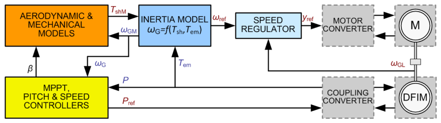
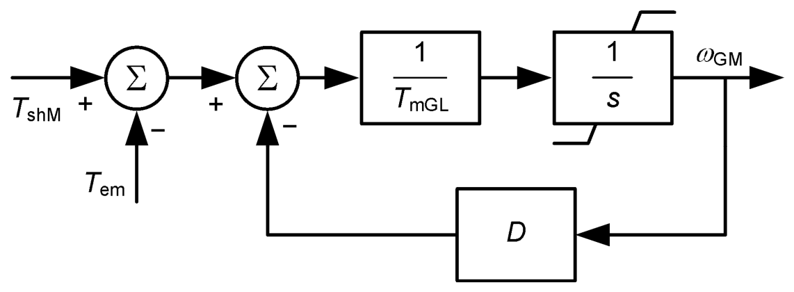
Based on the analysis conducted and preliminary laboratory investigations, the absence of a torque sensor (a torque sensor was not included in the design of the SWTE system at the LINTE^2 laboratory) and the availability of the generator angular velocity signal (ω_G) indicate that the most effective approach to modeling the inertia of the generator rotor in the MWT is method VII, incorporating an inertia model coupled with a rotational speed controller. The generator inertia model implemented enables real-time estimation of the rotor’s angular velocity (ω_GM) under specific operating conditions of the WT. This estimated velocity serves as the reference input (ω_ref = ω_GM) for the speed controller governing the shaft of the MG set, which in turn regulates the power converter supplying the motor. The speed controller was implemented in the motor converter controller (MCC)—Figure 9.

The MCC unit measures angular velocity using an absolute encoder. This controller operates at a significantly higher sampling frequency of 16 kHz compared to the SWTE controller (1 kHz), which allows for better control performance than the speed controller implemented in the SWTE simulation computer. The controller achieves shorter response times and higher regulation accuracy, with reduced oscillations. The limitations of the controller in the simulation computer result, among other things, from the lower sampling frequency (1 kHz) and the use of filters in the measurement circuits (10 ms ≤ T ≤ 20 ms). As a result, dynamic operating conditions induce noticeable angular velocity oscillations originating from the control system itself, preventing sufficiently fast and non-oscillatory responses. These effects were clearly observed during experimental validation of the speed controller implemented in the SWTE control unit. An important aspect to consider is that the frequency spectrum of the simulated mechanical torque on the shaft in the shaft model extends into higher frequencies than the transmission bandwidth of the speed signal from the inertia model, which is limited by the applied filter.

The DFIM is a component of the SWTE system. The DFIM is controlled by a simulated mechanical torque (T_sh) applied to the generator rotor shaft within the shaft model. This control is executed via the inertia model and the rotational speed controller of the machine shaft assembly. The inertia model is coupled with the measured electromagnetic torque (T_em) in the DFIM. The electromagnetic torque depends on the electrical power of the DFIM, which is regulated by models of active and reactive power controllers. Correct determination of the electromagnetic torque signal $T_{\mathrm{e}\mathrm{m}}$ is essential for accurate WT modeling using the SWTE.

The electromagnetic torque $T_{\mathrm{e}\mathrm{m}}$ in the generator of the SWTE can be determined in the SWTE simulation computer based on measurements of stator power, rotor speed, and slip. However, a more accurate determination of the electromagnetic torque was achieved using the rotor current components in the dq reference frame, available in the converter control unit, along with the estimated values of the coupled flux linkages. In the case of the SWTE system described, due to the use of this signal $T_{\mathrm{e}\mathrm{m}}$ within the control loop implemented directly in the converter controller, it is effectively immune to disturbances typically introduced by the switching transients of the converter’s power transistors.

6. Validation Studies

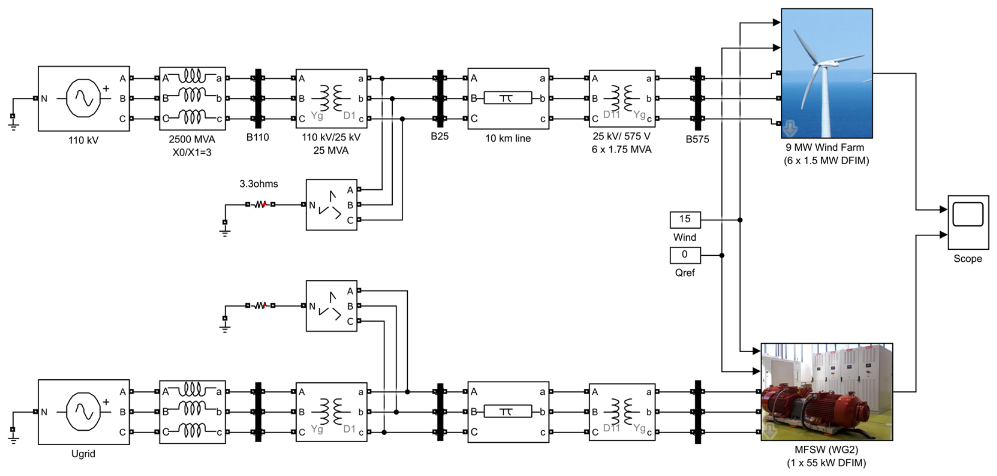
The validation aimed to demonstrate the capability of the SWTE to operate in electrical connection with other electrical devices, enabling the investigation of WT behavior within a power grid environment scaled to a nominal voltage of 400 V. The schematic of the validation model is shown in Figure 10.

As a RWFM, the Wind Farm—DFIG Average Model available in MATLAB Simulink R2015a was used. The wind farm consists of six WTs GE 1.5 equipped with doubly fed induction generators (DFIG). The turbines are connected to the HV grid via an LV/MV transformer, an MV transmission line, and an MV/HV transformer. The model is based on the methodology presented in [34] and developed by the authors of [35,36]. Additional components and configurations were adapted from [37,38]. For the purpose of validation, the model was modified by disabling the mechanical subsystem of the WT and replacing the drive control of the DFIG with a predefined torque input. The MPPT module was configured to operate at a fixed reference value of the speed controller, set to 1.2 (as previously described). The RWFM is represented by an aggregated model consisting of six identical WT units operating under identical conditions. Functionally, this configuration corresponds to a single WT model with six times the nominal power rating. During the validation study, the following quantities were monitored for both the RWFM and the model of the SWTE: mechanical torque on the shaft (T_sh), electromagnetic torque (T_em), generator angular velocity (ω_G), stator power (P_stat), power delivered to the grid (P_G), stator voltage (U_stat), and grid voltage (U_grid). Differences were observed in the waveforms of angular velocity, electromagnetic torque, stator power, and power delivered to the grid between the compared models. The maximum root mean square error (RMSE), calculated within a 10 ms moving window during steady-state and slowly varying operating conditions, as well as during and after transient disturbances, was used to quantify the accuracy of the simulation.

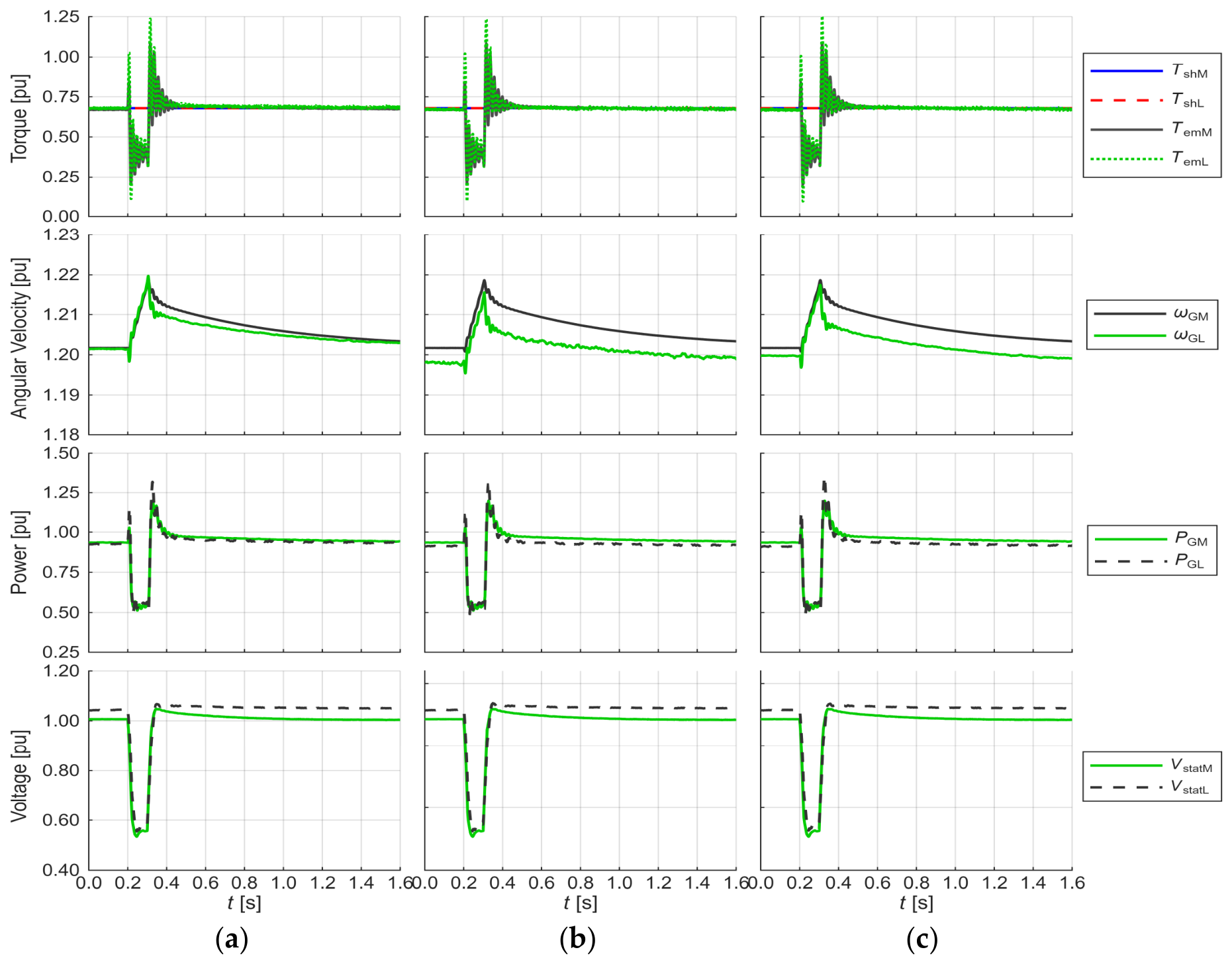
Figure 11 shows waveforms of torque, angular velocity, power, and voltage for the RWFM and the SWTE model during and after a grid voltage disturbance, evaluated using three selected inertia modeling methods:

• Application of a scaling function with a controller (VI—proprietary method),
• Application of an inertia model with a speed controller (VII—proprietary method),
• Compensation based on derivative feedback of angular velocity, implemented using a weighted moving average filter (IV according to [15]).

The disturbance applied was a step-type voltage sag in the 110 kV grid, reducing voltage by 50% for a duration of 0.12 s. The magnitude of the voltage sag was adopted in accordance with the original Simulink model to amplify the dynamic effects associated with the inertia of rotating components. Although such a voltage sag may present a potential risk to the converter, this factor was deliberately excluded from the scope of the dynamic analysis.

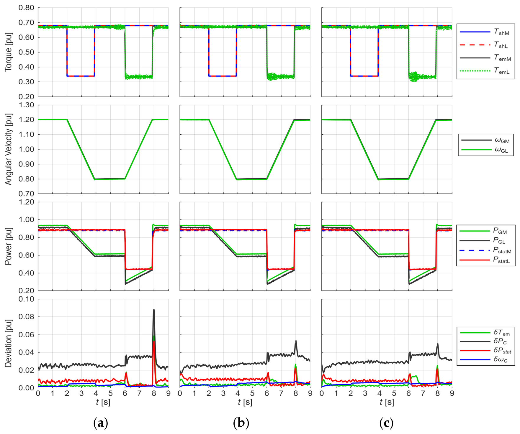
Figure 12 presents waveforms following a disturbance caused by a step change in mechanical and electromagnetic torque, evaluated using the same inertia modeling methods. Additionally, RMSE waveforms for torque, power, and angular velocity are included to illustrate deviations between the simulation results of the RWFM and the model of SWTE. The waveforms were recorded for a case with fixed inertia constants: H_L = 0.56 s and H_G = 0.96 s—parameters corresponding to the SWTE MG set investigated in this study and to the GE 1.5 generator. 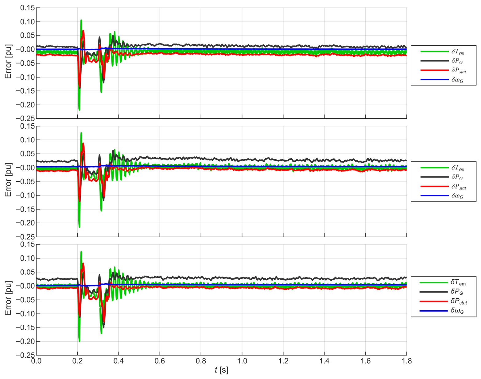The corresponding error waveforms are presented in Figure 13.

Figure 13 presents the recorded waveforms of instantaneous error following a voltage disturbance in the HV grid. As shown in Figure 13, the instantaneous error following the grid voltage disturbance reaches significant values during the first two oscillations, but these are rapidly damped. The absolute deviation of the SWTE generator’s electromagnetic torque from that of the modeled wind system reaches up to 0.21 p.u. in the first oscillation peak. After approximately 20 ms, the absolute error drops below 0.03 p.u. Disturbances with very steep rise characteristics result in a substantial mismatch between the model of WTE and the MWT during the first 20 ms. The instantaneous error waveforms following the voltage sag appear very similar across all three evaluated compensation methods.

Table 4. Accuracy comparison of the investigated inertia-compensation methods: maximum root mean square errors of the generator angular velocity, stator active power and active power supplied to the grid for different inertia constants, together with uncertainty estimates for the voltage-sag test. The gray background indicates the tested inertia constant values. The smallest error values are highlighted in bold, the largest in red.

	Root Mean Square Error [p.u.]
	δωG			δPstat			δPG
Generator inertia constant:
WTE HL [s]	0.56	0.3	0.6	0.56	0.3	0.6	0.56	0.3	0.6
modeled WT HM [s]	0.96	1.2	0.3	0.96	1.2	0.3	0.96	1.2	0.3
Inertia compensation method	Root mean square error of simulation in static and slowly changing states
Inertia model (VII)	0.006	0.006	0.006	0.016	0.016	0.010	0.029	0.028	0.030
Scaling function (VI)	0.005	0.006	0.012	0.011	0.030	0.015	0.028	0.072	0.031
Compensation using derivative of angular velocity feedback (IV)	0.006	0.009	0.016	0.016	0.015	0.010	0.031	0.031	0.030
Inertia compensation method	Root mean square error of simulation in dynamic states
Inertia model (VII)	0.008	0.008	0.012	0.023	0.023	0.017	0.053	0.054	0.046
Scaling function (VI)	0.005	0.010	0.018	0.052	0.074	0.025	0.089	0.119	0.066
Compensation using derivative of angular velocity feedback (IV)	0.007	0.009	0.028	0.022	0.021	0.036	0.050	0.047	0.078

Note: Maximum RMSE values calculated in a 10 ms moving window.

summarizes the maximum moving-window RMSE values obtained under static, slowly varying, and dynamic operating conditions. Validation studies were carried out for ${\displaystyle \frac{H_{\mathrm{M}}}{H_{\mathrm{L}}}}\in \left\{0.5; 1.71;·4\right\}$ ($\left(H_{\mathrm{L}};H_{\mathrm{M}}\right)\in \left\{\left(0.6;0.3\right);\left(0.56;0.96\right);·\left(0.3;1.2\right)\right\}$[s]).

Table 5. Statistical uncertainty of RMSE for the voltage-sag test (Figure 13).

Inertia Compensation Method	δTem			δPstat
	RMSE [p.u.]	sboot [p.u.]	98% CI [p.u.]	RMSE [p.u.]	sboot [p.u.]	98% CI [p.u.]
Inertia model (VII)	0.0205	0.0052	[0.0078, 0.0316]	0.0163	0.0035	[0.0073, 0.0240]
Scaling function (VI)	0.0218	0.0049	[0.0106, 0.0327]	0.0231	0.0022	[0.0186, 0.0287]
Compensation using derivative of angular velocity feedback (IV)	0.0212	0.0054	[0.0079, 0.0327]	0.0172	0.0039	[0.0073, 0.0258]

Note: RMSE were calculated over the complete 0–1.8 s record (N = 72,001 samples) from the voltage-sag test shown in Figure 13. s_boot denotes the standard deviation of the bootstrap RMSE distribution, not run-to-run variability. The 98% confidence intervals were obtained from 10,000 moving-block bootstrap replications using 2000-sample blocks (50 ms). Because one time-series realization was available for each method, the intervals quantify uncertainty within the recorded realization and do not replace repeated independent experimental trials.

reports the whole-record RMSE values, bootstrap standard deviations, and 98% confidence intervals for the voltage-sag test.

Analysis of the results allows the accuracy of the angular velocity δω_G of the methods to be determined. The accuracy of angular velocity emulation using Method VI (scaling function) is better than 1.8%, and under steady-state conditions, better than 1.2% across the entire range of modeled inertia values. Method VII, which employs an inertia model, achieves corresponding accuracy levels of 1.2% and 0.6%, respectively. Method IV described in [15], based on derivative feedback of angular velocity with a weighted moving average, yields an RMSE of 2.8%, and under steady-state conditions, produces no higher than 1.6% across the full range of modeled inertia values. For comparison, the method described in [14], which uses an inertia emulator and electromagnetic torque estimated within the DFIM controller, achieves angular velocity emulation accuracy in a range of approximately 6–8%.

To quantify the uncertainty of the error estimates for the voltage-sag test shown in Figure 13, Table 4 was supplemented with Table 5—the whole-record RMSE values for the electromagnetic-torque error δT_em, and stator active-power error δP_stat, together with bootstrap standard deviations and two-sided 98% confidence intervals. Method VII yielded the lowest central RMSE estimates for both signals. However, the confidence intervals overlap, indicating comparable accuracy of the three methods and not providing evidence of statistically significant superiority based on this single disturbance realization.

The RMSE values for δT_em, δP_stat i δω_G under steady-state and slowly varying signal conditions are below 0.02 p.u. Under step-type torque disturbances, the error may reach approximately 0.025 p.u. for Methods VII and as found in IV, while for Method VI, the error rises to around 0.06 p.u. In the T_em waveform for Method IV [15], transient oscillations are observed with a period of 20 ms and an amplitude of up to 0.04 p.u. Similar oscillations are also present in Method VII, but with an amplitude approximately half as large.

7. Conclusions

This study addressed the problem of reproducing the inertial response of a full-scale wind turbine using a laboratory motor–generator set whose physical inertia differs from that of the modeled machine. Two approaches were developed. Method VI determines the required shaft torque using a conversion function derived from the equations of rotational motion and parameterized by the inertia constants of the modeled turbine and the laboratory set. Method VII introduces a numerical model of the generator inertia and uses the calculated angular velocity as the reference signal for the speed controller of the drive motor. Both approaches avoid the need to modify the rotating masses of the test bench and therefore preserve the scalability of the SWTE.

The comparative validation showed that the proposed methods provide more accurate reproduction of generator-speed dynamics than the selected derivative-feedback compensation method. For the investigated range of modeled inertia, Method VI limited the maximum angular-velocity RMSE to 1.8%, whereas Method VII reduced it to 1.2%. Under steady-state and slowly varying conditions, the corresponding errors did not exceed 1.2% and 0.6%, respectively. The reference method based on angular-velocity derivative feedback produced errors of up to 2.8%. The results also confirmed that Method VII offers the best overall agreement with the reference wind farm model, while avoiding direct differentiation of the measured speed signal. The experimental implementation of this method benefited from locating the speed controller in the motor converter controller, which operates at a higher sampling frequency than the real-time simulation platform.

The present study has several limitations. The investigation was conducted for one DFIM-based SWTE configuration and one reference wind farm model. The comparative tests covered a finite range of inertia constants, from 0.25H_L to 2H_L, and selected disturbances, including a temporary voltage sag and step changes in mechanical and electromagnetic torque. Furthermore, Method VI was evaluated using the validation models but was not implemented on the physical test bench because the existing WG2 setup is not equipped with a shaft torque sensor. The obtained accuracy levels may also depend on the sampling frequencies, signal transmission delays, measurement disturbances, and filtering adopted in the particular laboratory implementation.

Future work will include experimental verification of the torque-scaling method after extending the test bench with an appropriate shaft-torque measurement system. The validation will also be broadened to include additional wind turbine models, operating points, grid disturbances, and a wider range of equivalent inertia constants. Further investigations will address the robustness of both methods to measurement noise, communication delays, controller bandwidth limitations, and parameter uncertainty. The final objective is to establish a general procedure for configuring scalable WTEs that can reproduce the inertial and electromechanical response of different wind turbine technologies under realistic power-system operating conditions.