1. Introduction
With rapid economic development, urbanization, population concentration, and continuous changes in electricity consumption structures, regional electricity demand has continued to grow [
1]. This growth is reflected not only in increasing total electricity consumption but also in increasingly diversified demand structures, more complex consumption patterns, and more pronounced load fluctuations. Existing studies have shown that electricity demand is closely associated with socioeconomic factors such as economic growth, urbanization, and population size, while peak load is also associated with weather conditions and building electricity-use behavior [
1,
2]. The uncertainty of load variation increases the difficulty of maintaining power supply–demand balance, grid dispatch, and operational security, thereby imposing higher requirements on the safe and stable operation of power systems [
3]. In power-system planning and operational management, accurately characterizing load variation at different temporal scales provides an important basis for generation scheduling, equipment maintenance, resource allocation, and demand-side management [
4,
5,
6]. Therefore, identifying the multiscale characteristics of regional power load and its associations with external factors is important for improving grid operation efficiency, supporting load forecasting, facilitating renewable energy accommodation, and informing differentiated load-management strategies.
Complex power-load series often contain trend, periodic, and random disturbance components. Analyzing the original load series as a whole cannot explicitly distinguish structural characteristics occurring at different temporal scales. To separate components with different temporal characteristics, signal decomposition methods have gradually been introduced into load studies [
7]. Zhu et al. [
8] adopted an EMD–FbProphet–LSTM method to forecast daily electricity consumption at the enterprise level, while Semero et al. [
9] used empirical mode decomposition (EMD) to decompose short-term microgrid load and improve forecasting performance. Although EMD can adaptively decompose nonstationary signals, it is susceptible to mode mixing when processing intermittent fluctuations. Ensemble empirical mode decomposition (EEMD) was subsequently developed by adding white noise to the original signal and has been applied to short-term load forecasting [
10,
11]. However, the introduced noise may also affect the representation of the original fluctuation characteristics. In comparison, variational mode decomposition (VMD) decomposes a signal into several band-limited mode components by constructing and solving a constrained variational problem. Its non-recursive formulation provides relatively stable decomposition performance and improved resistance to mode mixing and noise interference [
12], and it has been increasingly applied in power-load analysis and forecasting [
13].
In addition to load decomposition, identifying associations between load variation and external factors is essential for interpreting regional electricity-demand patterns. Existing studies commonly use feature-analysis methods to screen load-related variables and reduce the interference of weakly associated or redundant variables in model inputs and result interpretation. Pearson correlation has been widely used to characterize linear associations between power load and candidate variables and to select highly correlated predictors [
10]. Information-theoretic methods have also been employed to capture more general statistical dependencies that may not be fully represented by linear correlation. These studies provide an important basis for load-factor identification, but most are primarily oriented toward improving forecasting accuracy. Meteorological, calendar, and socioeconomic variables are generally treated as unified model inputs, while the differences in their associations with specific load components and temporal scales receive comparatively limited attention [
10,
14]. For regional load, meteorological variables may be associated with both seasonal low-frequency variation and intraday short-cycle fluctuations. Previous studies have shown that variables such as temperature, precipitation, and sunshine are associated with electricity demand across different intraday periods and seasonal conditions [
15,
16]. Industrial and consumption indicators more commonly characterize changes in monthly economic activity, whereas industrial structure, economic scale, and energy structure provide longer-term contextual information at the annual scale [
17]. Without distinguishing the scale-specific association patterns between load components and external variables, relationships occurring at different temporal scales may be conflated, reducing the interpretability of factor analysis.
Recent decomposition-based load studies mainly use EMD, EEMD, VMD, and related methods as preprocessing tools and evaluate their value through forecasting accuracy, while interpretable load studies generally assess feature importance or select external variables within predictive models [
18,
19]. These approaches provide useful predictive information but rarely compare the associations obtained from the original load series with those identified from frequency-specific load components using the same analytical procedure. Regional electricity-demand studies also tend to focus on aggregate or spatial differences rather than on how meteorological and socioeconomic associations are distributed across temporal scales [
20,
21]. Studies incorporating ambient temperature into residential electricity-demand forecasting further indicate that the relevance of external variables depends on temporal resolution and electricity-use context [
22].
Accordingly, the contribution of this study does not lie in proposing new VMD, Pearson correlation, or mutual-information algorithms individually, but in integrating them into a unified multiscale association framework. The original load series is retained as a common baseline, and the same Pearson correlation and MI procedures are applied to both the original load and the decomposed modes. This design allows the overall associations observed in the original series to be compared with the temporal components in which they are concentrated. Hourly analyses are conducted separately as two within-region cases, whereas regional comparisons are limited to the temporally aligned monthly and annual datasets. The framework is descriptive and is intended to identify scale-specific contemporaneous associations rather than causal effects, lagged responses, or validated forecasting benefits. The objectives are therefore to (1) characterize the multiscale structures of regional power load; (2) identify the temporal components in which meteorological and socioeconomic associations are concentrated; and (3) describe regional differences using the aligned monthly and annual datasets.
2. Study Area, Data, and Technical Framework
2.1. Overview of the Study Area
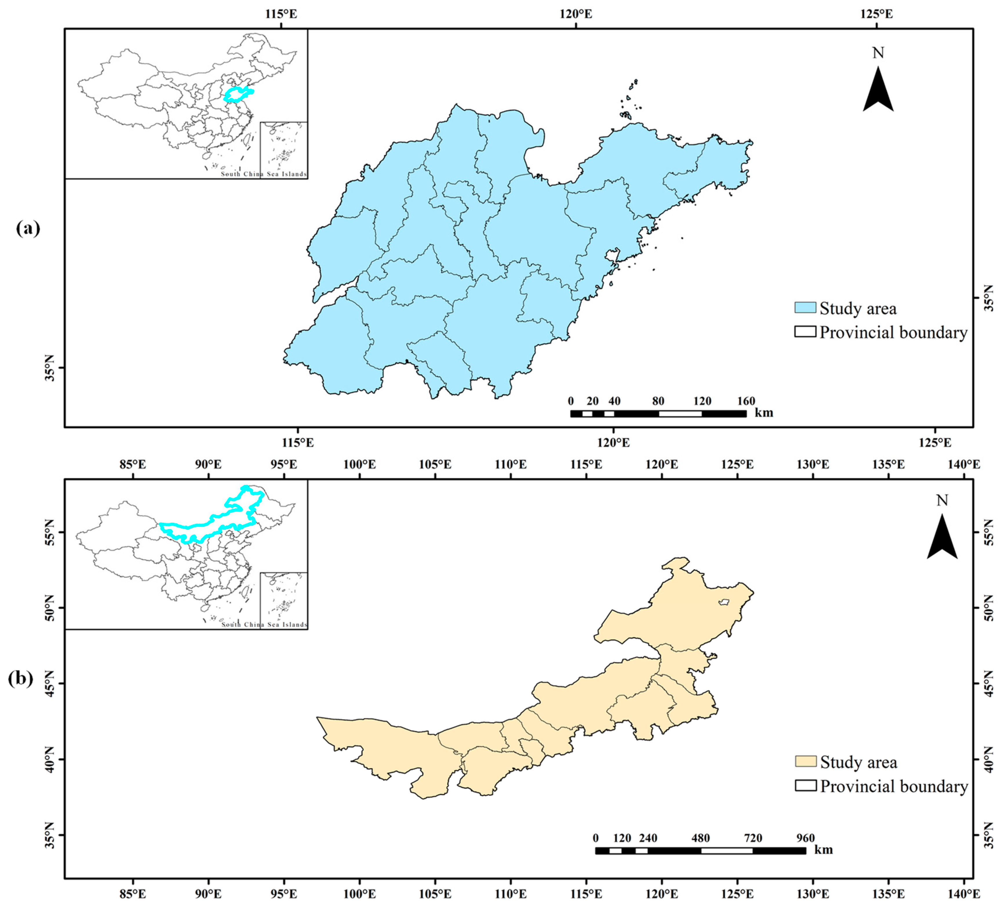
This study selects Shandong Province and Inner Mongolia Autonomous Region as the study areas, and their locations are shown in
Figure 1. Both regions have a strong foundation of industrial electricity consumption and relatively high regional power load levels, but there are obvious differences in meteorological conditions, industrial structure, and socioeconomic activities. Existing studies have shown that temperature variation, cooling demand, and heating demand significantly affect residential electricity consumption and regional load variation, and that such effects differ across climatic zones and between urban and rural electricity consumers [
23,
24]. Shandong is located in the eastern coastal region of China, with relatively humid climatic conditions and obvious high-temperature and high-humidity characteristics in summer. Cooling load and residential electricity consumption show strong seasonality. Meanwhile, Shandong has a complete industrial system and a solid manufacturing foundation, and socioeconomic activities such as the service industry, urban commercial activities, residential consumption, and transportation logistics are relatively active. Therefore, load variation is more likely to reflect the compound characteristics under the combined effects of industrial production, urban consumption, and meteorological seasonality.
Inner Mongolia is located in the northern inland region of China and has typical continental climatic characteristics, with cold winters of long duration. Heating demand and the low-temperature background have obvious effects on load variation. In its industrial structure, resource-based industries and energy-intensive industries, such as coal, metallurgy, and energy chemical industries, account for a relatively high proportion, making the industrial base-load characteristics more prominent. Relevant studies have pointed out that Inner Mongolia is an important energy-supply region in China, with obvious characteristics of coal and electricity transmission outward, as well as strong demand from energy-intensive industries. In addition, the types of socioeconomic activities differ between the two regions: Shandong has stronger population agglomeration and urban consumption activities, whereas Inner Mongolia has characteristics involving resource industries, pastoral-area economy, and heating demand. Conducting a multiscale comparison of the two regions is helpful for identifying differences in the association structures of regional power load under different meteorological and socioeconomic backgrounds.
2.2. Data Sources and Preprocessing
This study uses load, meteorological, and socioeconomic data from Shandong and Inner Mongolia at hourly, monthly, and annual resolutions. The load datasets were provided by China Renewable Energy Engineering Institute Corporation Limited (CREEI). The meteorological data were derived from the national meteorological-station database of the China Meteorological Administration (CMA), while the socioeconomic data were obtained from the National Bureau of Statistics of China (NBS).
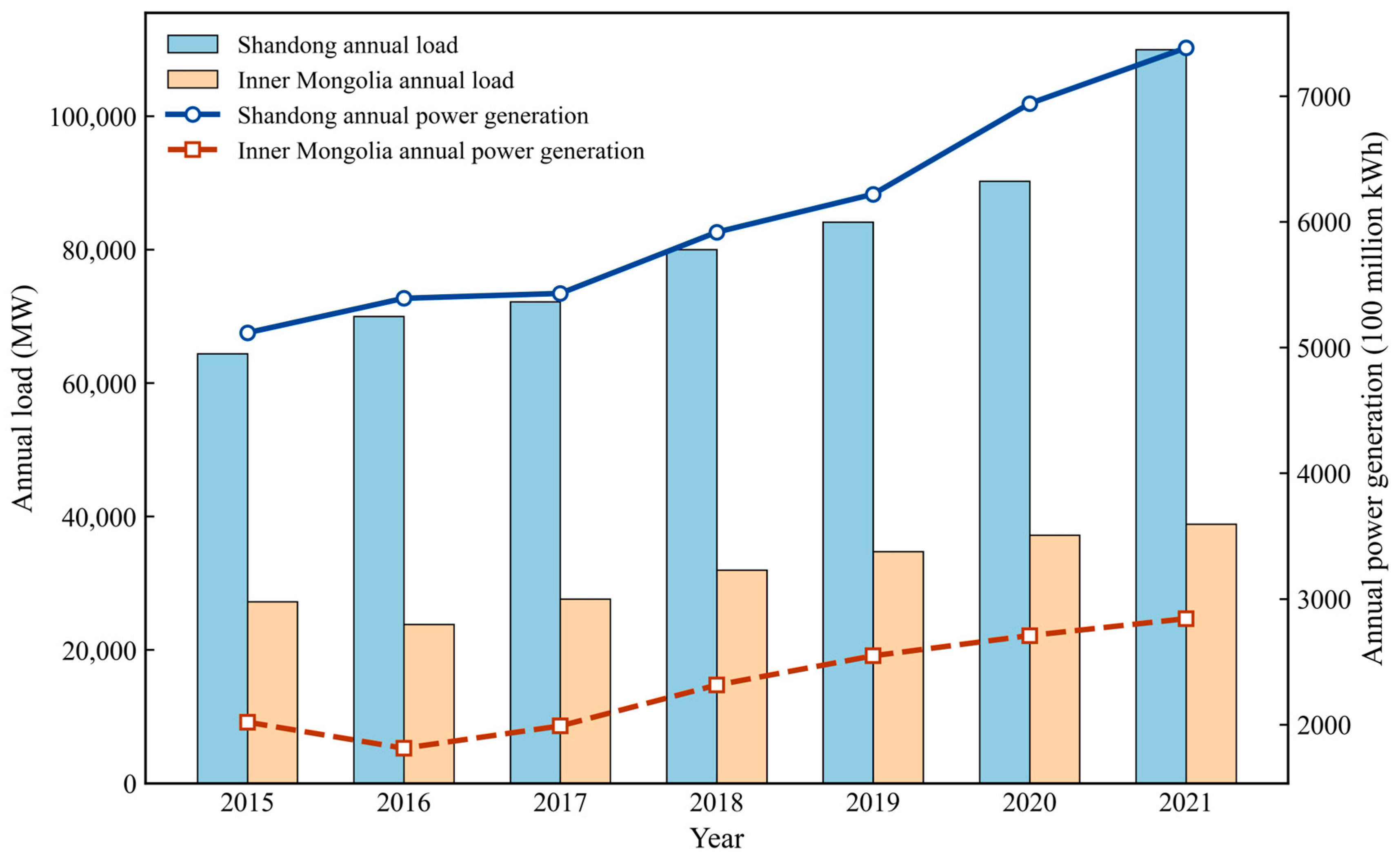
The meteorological data used in this study were supplied as province-level regional-average series derived from CMA station records. Individual station observations and station metadata were not included in the delivered dataset; therefore, no additional station selection, spatial interpolation, or station-weighted aggregation was performed by the authors. The publicly sourced meteorological and socioeconomic data can be accessed through the China Meteorological Data Service Centre and the National Data platform of the NBS, respectively. The CMA system provides access to surface meteorological datasets, while the NBS platform provides monthly, annual, and regional socioeconomic indicators. The hourly load series represents the province-level load recorded at one-hour intervals and supplied directly by CREEI. The monthly load series consists of one provider-defined province-level load value for each calendar month. It was supplied independently of the hourly series and was not calculated by the authors as a monthly mean, maximum, sum, or other aggregation of the hourly load data. Annual load variation is described using annual maximum load and annual electricity consumption.
Owing to the different availability periods of the provincial hourly load data, the Shandong hourly dataset covers 2024, whereas the Inner Mongolia hourly dataset covers 2015–2021. The hourly analyses are therefore conducted separately within each region. The monthly and annual datasets for both regions cover 2015–2021 and are used for regional comparison. The dataset composition and variable definitions are summarized in
Table 1,
Table 2,
Table 3 and
Table 4.
The load series were independently normalized to [0, 1] for each region and temporal resolution using Min–Max normalization:
where
is the original load value at time
,
and
are the minimum and maximum values of the corresponding load series, respectively. The monthly load data are provider-defined monthly indicators rather than aggregates derived from the hourly series. Annual load variation is described using annual maximum load and annual electricity consumption.
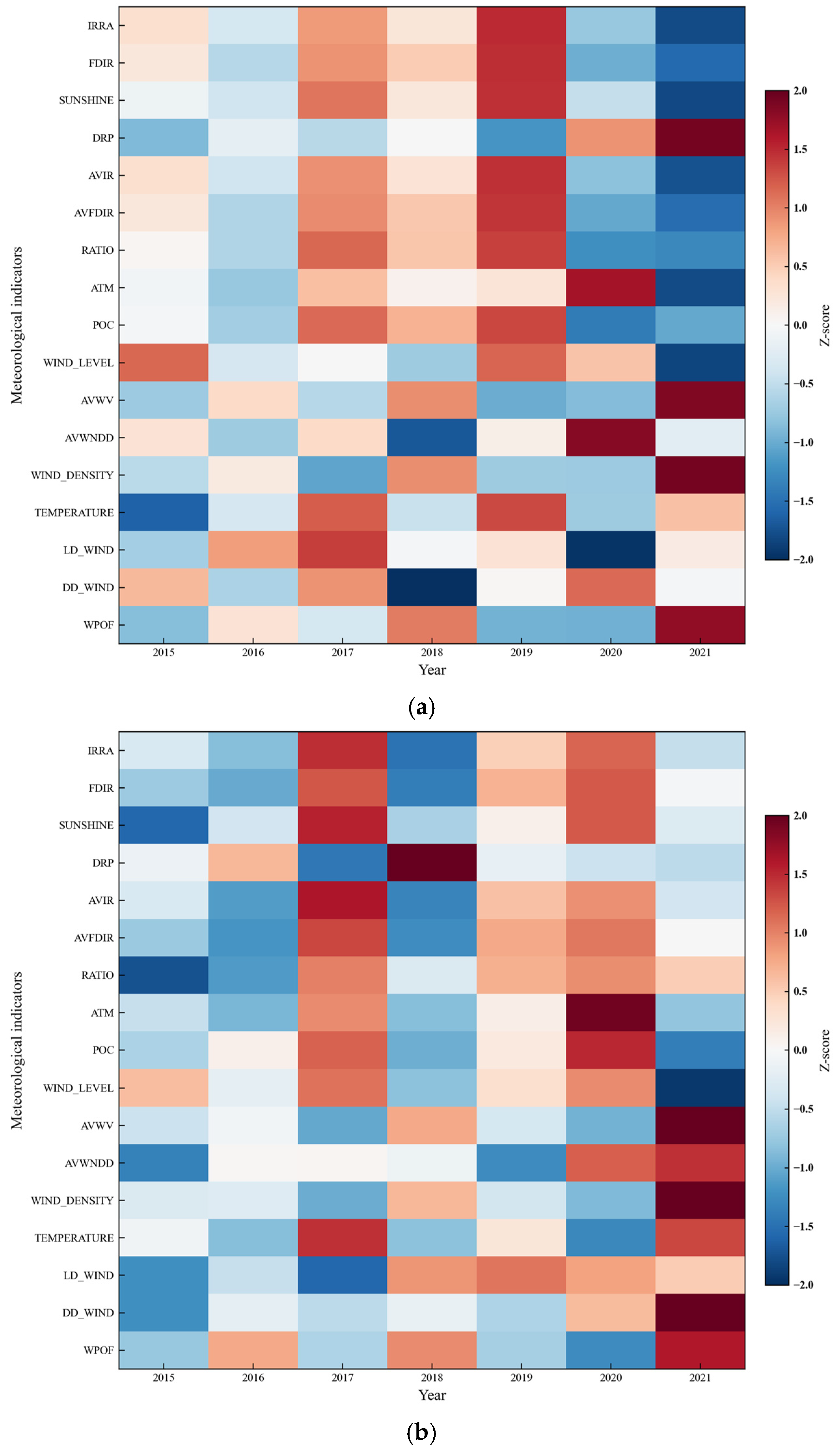
Data-quality control included chronological ordering, alignment of the load and external-variable series using common timestamps, inspection for missing observations, and examination of zero-valued load records. No missing observations were identified. Six dates in the Inner Mongolia hourly dataset contained zero-valued records; these records were retained in the main analysis, and their influence was examined through sensitivity analysis. For the monthly and annual meteorological datasets, cumulative variables, including IRRA, FDIR, SUNSHINE, and DRP, were aggregated by summation, whereas continuous-state variables were aggregated by averaging. Other derived indicators retained their original definitions.
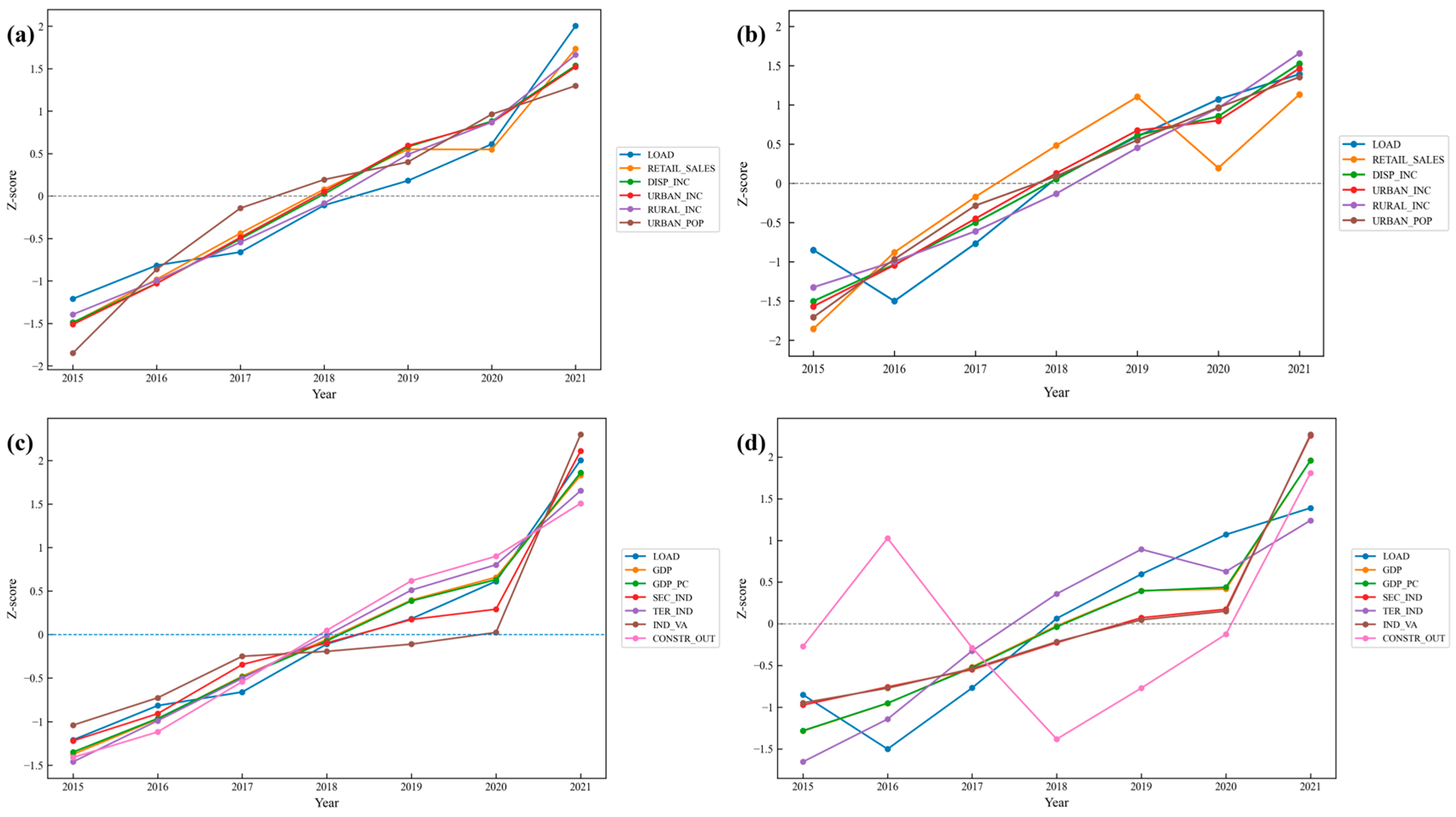
To compare annual variables with different units and magnitudes, Z-score standardization was applied:
where
denotes the value of variable
in year
,
and
denote its mean and standard deviation over 2015–2021, respectively. Z-score standardization was used only for the annual indicators presented in the annual-scale analysis and was not applied to the hourly or monthly VMD.
2.3. Technical Framework and Research Methods
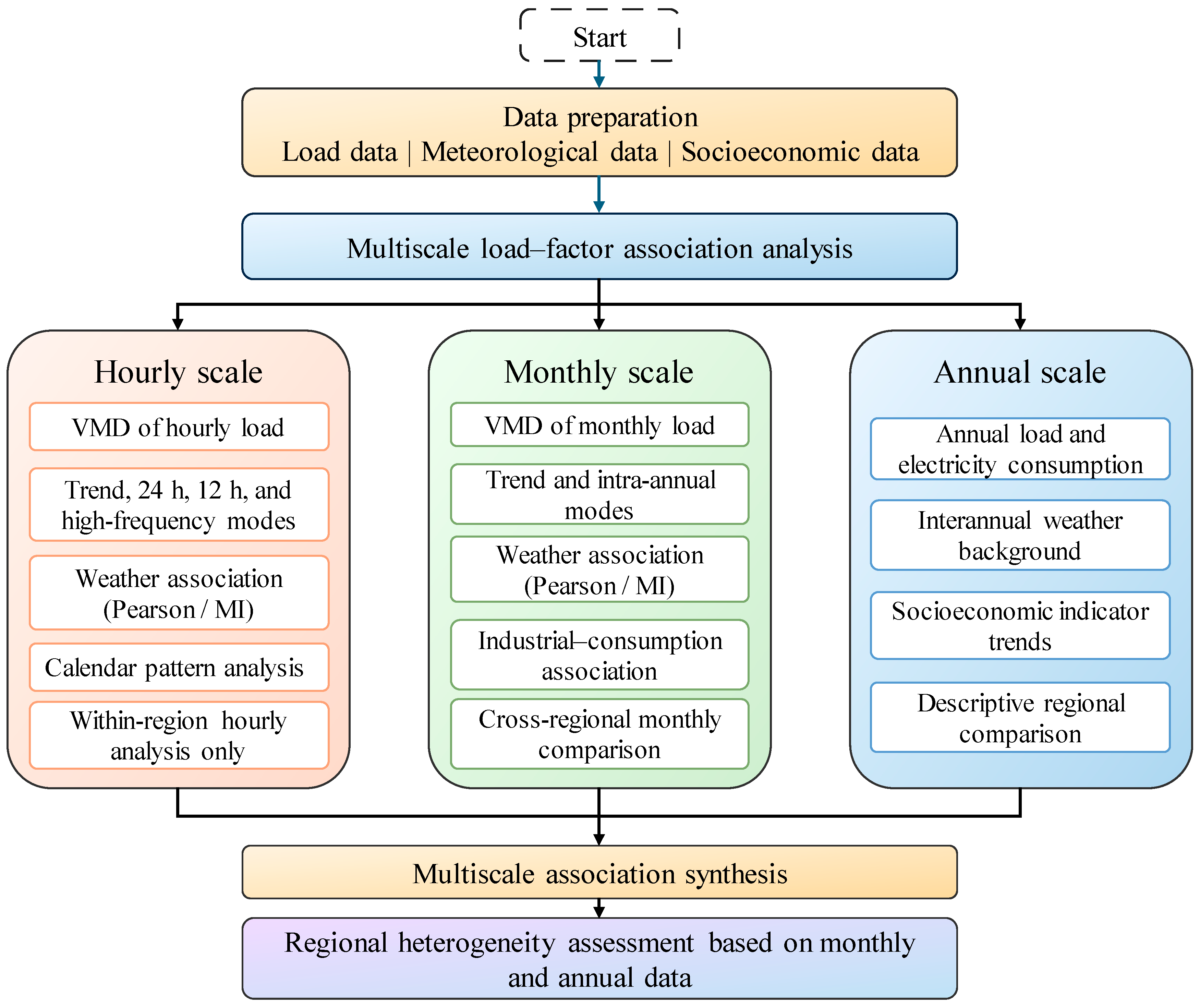
To investigate the multiscale associations between power load and meteorological and socioeconomic factors in Shandong and Inner Mongolia, this study develops an “hourly–monthly–annual” analytical framework. The research procedure is illustrated in
Figure 2 and consists of six steps.
- (1)
Data preparation: Load, meteorological, and socioeconomic data are collected and organized to construct hourly, monthly, and annual datasets.
- (2)
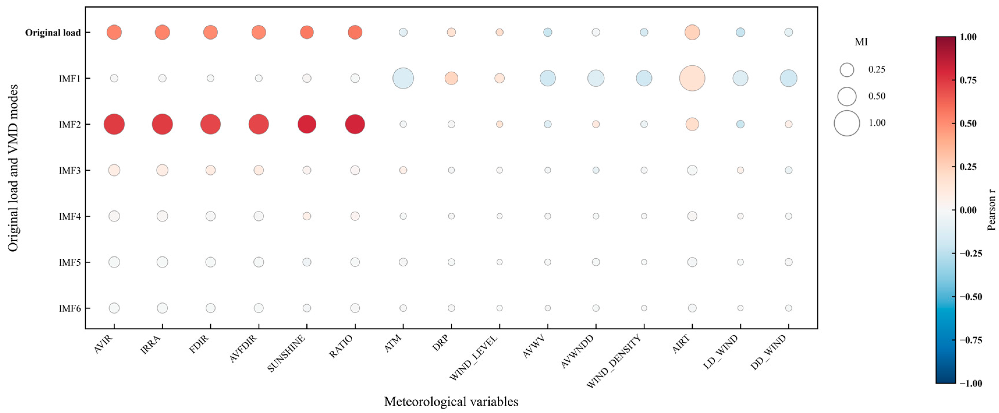
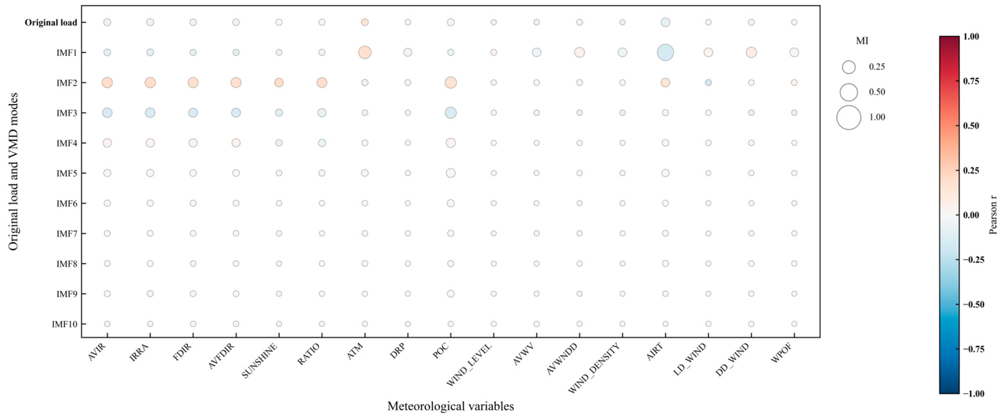
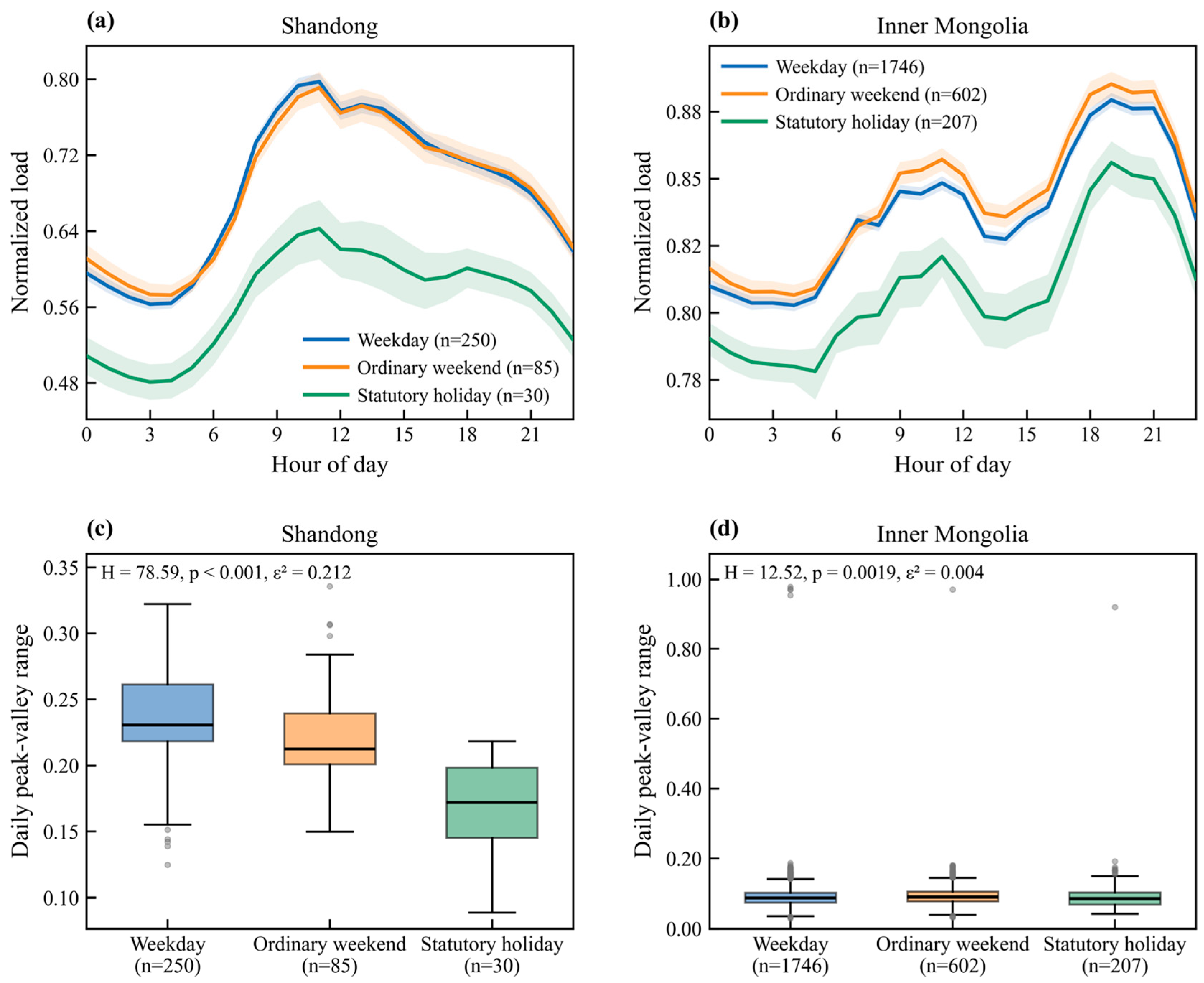
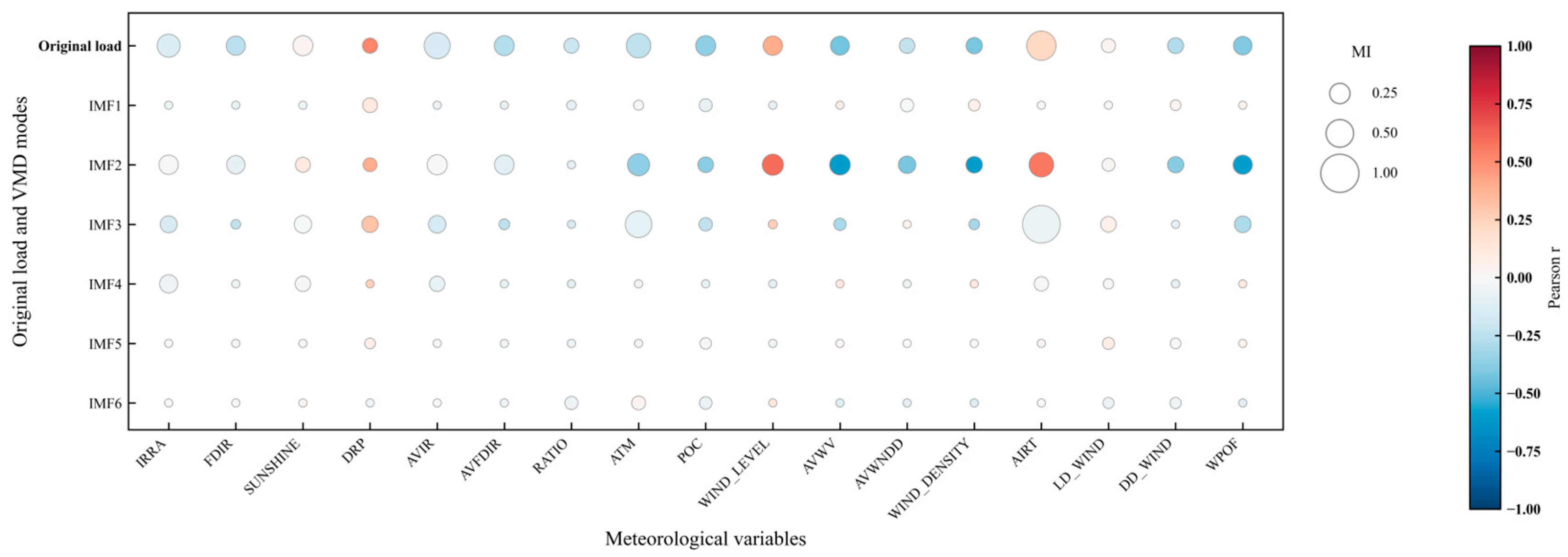
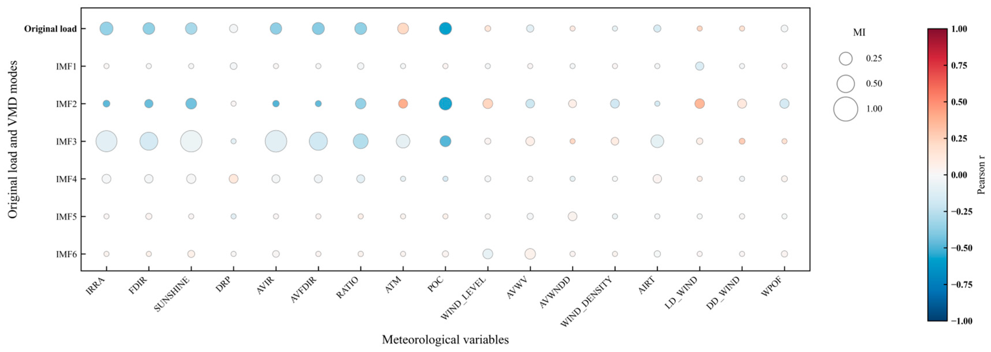
Hourly-scale analysis: VMD is applied to the hourly load series of each region separately to identify low-frequency trends, 24 h and 12 h periodic components, and high-frequency modes. Pearson correlation and mutual information are then used to examine the contemporaneous associations between meteorological variables and the decomposed load modes, followed by a comparison of intraday load profiles across different date types within each region.
- (3)
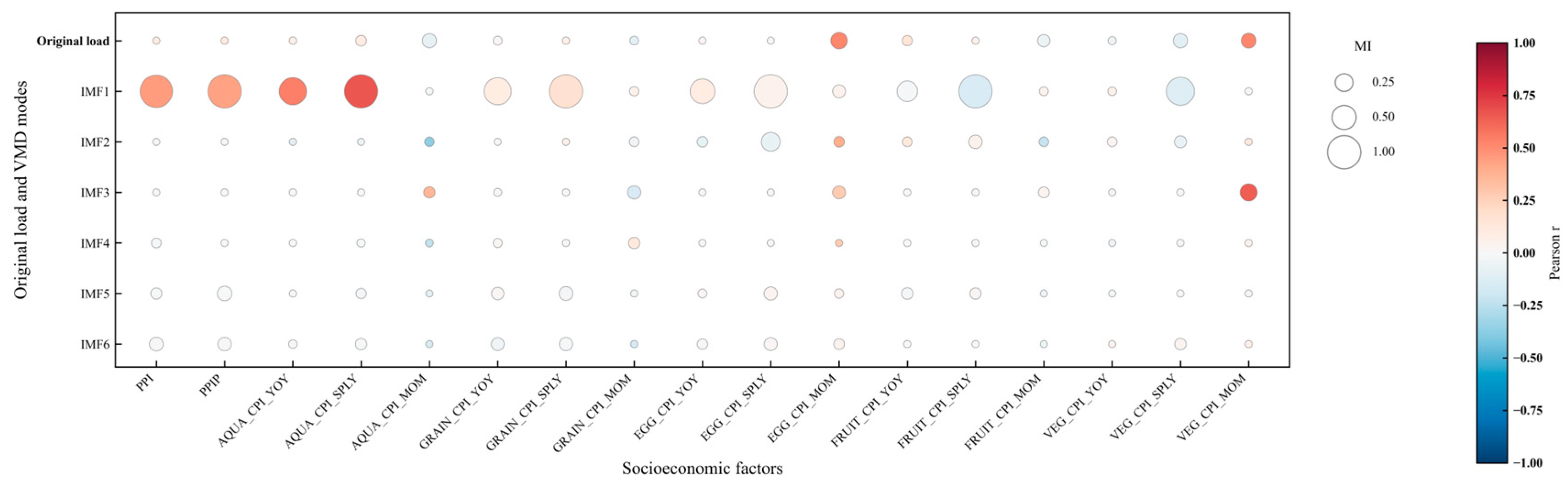
Monthly-scale analysis: VMD is applied to the monthly load series to identify low-frequency trends and intra-annual fluctuation modes. The associations of meteorological, industrial, and consumption-related variables with the monthly load modes are then examined using Pearson correlation and mutual information.
- (4)
Annual-scale analysis: Descriptive comparisons are conducted using annual maximum load, annual electricity consumption, meteorological conditions, and socioeconomic indicators to characterize the regional backgrounds associated with long-term load changes. Owing to the limited number of annual observations, this step is used only for descriptive interpretation rather than statistical inference.
- (5)
Multiscale association synthesis: The hourly, monthly, and annual results are integrated to summarize how meteorological, industrial, and consumption-related variables are associated with load characteristics at different temporal scales.
- (6)
Regional heterogeneity assessment: Regional differences between Shandong and Inner Mongolia are evaluated mainly on the basis of the temporally aligned monthly and annual datasets. The hourly results are interpreted separately as within-region cases and are not used as direct evidence of cross-regional heterogeneity.
2.3.1. VMD Method
Variational mode decomposition (VMD) is a non-recursive signal decomposition method proposed by Dragomiretskiy and Zosso. By constructing a constrained variational model, this method decomposes the original nonstationary signal into several mode components with finite bandwidth, and each mode is distributed around a different center frequency [
15]. Compared with recursive decomposition methods such as EMD, VMD shows better performance in suppressing mode mixing and reducing noise interference. In power load studies, VMD is commonly used to decompose complex load sequences, reduce the nonstationarity of the original sequence, and extract load variation components at different frequency scales [
13].
VMD first calculates the analytic signal of each mode component
through the Hilbert transform to obtain the unilateral spectrum.
The analytic signal of each mode is then mixed with its corresponding center frequency term
, so that the spectrum of each mode is shifted to the corresponding baseband.
The bandwidth of each mode signal is then estimated by calculating the squared
norm of the gradient of the demodulated signal based on the Gaussian smoothness criterion. Accordingly, the constrained variational model is formulated as follows:
where
denotes the partial derivative with respect to time (t),
denotes the set of decomposed mode components,
denotes the set of center frequencies corresponding to each mode component, and ∗ denotes the convolution operation.
The Lagrange multiplier and the quadratic penalty factor are introduced to transform the constrained variational problem into an unconstrained variational model.
To obtain the optimal solution of Equation (7), VMD adopts the alternating direction method of multipliers. With the cyclic updates in Equations (8) and (9), each decomposed signal
and its corresponding center frequency
are iteratively updated.
When the convergence criterion in Equation (10) is satisfied, the iterative procedure is terminated.
The quality of the VMD results was evaluated using the orthogonality index (OI), relative reconstruction error (RRE), and mode mixing index (MMI):
where
is the original load series,
is the mode,
is the number of modes, and
is the normalized one-sided power spectrum of
. Lower OI, RRE, and MMI values indicate better mode orthogonality, reconstruction accuracy, and spectral separation, respectively.
Each mode was further characterized by its center frequency, dominant period, amplitude, and standard deviation. The center frequency was obtained from the converged frequency estimate of the VMD algorithm. The remaining indicators were calculated as
where
is the frequency corresponding to the largest non-zero spectral peak,
is the sequence length, and
is the mean of mode
. The dominant periods are expressed in hours for hourly data and months for monthly data. Detailed parameter settings and sensitivity analyses are presented in
Section 2.4.
2.3.2. Pearson Correlation and Mutual Information Analysis
To characterize the associations between different load modes and external factors, the Pearson correlation coefficient and mutual information (MI) are jointly employed. The Pearson correlation coefficient measures the direction and strength of the linear association between two variables, whereas MI measures their general statistical dependence, including both linear and nonlinear dependence. Let the decomposed load-mode sequence be
and the influencing factor sequence be
. The Pearson correlation coefficient is calculated as follows:
where
When
, the two variables are positively correlated; when
, the two variables are negatively correlated. The closer
is to 1, the stronger the linear correlation.
MI measures the general statistical dependence between two variables and is defined as follows:
where
is the joint probability density function, and
and
are the marginal probability density functions, respectively. When
, the two variables are independent of each other. The larger the mutual information value, the stronger the degree of information dependence between them. Since the research variables are mostly continuous sequences, mutual information can be estimated using a nonparametric method based on
nearest neighbors to reduce the influence of binning methods on the results [
25].
Considering the serial dependence of the monthly series, the uncertainty of the monthly Pearson correlation coefficients was further evaluated using a circular moving-block bootstrap [
26]. For each load–factor pair, the two series were resampled jointly to preserve their contemporaneous relationship and local temporal dependence. Let
denote the paired monthly observations. A circular block of length
beginning at position
is defined as
For the
-th bootstrap sample,
blocks were randomly selected with replacement and concatenated, after which the resulting sequence was truncated to the original sample length
. The Pearson correlation coefficient was recalculated for each bootstrap sample:
The percentile confidence interval was obtained from the empirical distribution of the bootstrap correlation coefficients:
where
denotes the
-th quantile of the bootstrap distribution. A Pearson association was recorded as retained by the unadjusted block-bootstrap analysis when its unadjusted 95% confidence interval did not include zero. The bootstrap procedure was applied only to the monthly Pearson coefficients, whereas the MI results were retained as descriptive measures of statistical dependence.
2.3.3. Calendar-Related Statistical Analysis
Calendar-related differences were evaluated among weekdays, ordinary weekends, and statutory holidays. The mean 24 h load profiles and their 95% confidence intervals were estimated using 4000 nonparametric bootstrap resamples at the daily-profile level. The daily peak-to-valley range was calculated as
where
denotes the load at hour
on day
. Differences among the three date categories were assessed using the Kruskal–Wallis test [
27]. When the overall test was significant, Dunn’s pairwise test with the Holm correction was applied, and epsilon squared was used to quantify the effect size:
where
is the Kruskal–Wallis statistic,
is the number of groups, and
is the total number of daily profiles. A sensitivity analysis was conducted after excluding the six zero-valued dates in the Inner Mongolia dataset.
2.4. Parameter Settings and Sensitivity Analysis
The number of modes K was selected separately for each load series by jointly considering the orthogonality index (OI), relative reconstruction error (RRE), mode mixing index (MMI), and the interpretability of the center-frequency and dominant-period structures. The other VMD parameters were fixed at α = 2000, τ = 0, DC = 0, init = 1, a convergence tolerance of 1 × 10
−7, and a maximum of 500 iterations. Based on the overall evaluation, K = 6 was selected for the Shandong hourly load, K = 10 for the Inner Mongolia hourly load, and K = 6 for both monthly load series. The detailed results are reported in
Table 5.
After determining K, the penalty parameter α was further tested at 1500, 2000, and 2500. The dominant periods of the corresponding modes remained unchanged under the three settings. Considering the overall performance of OI, RRE, and MMI, as well as the need for consistent parameter settings across regions and temporal scales, α = 2000 was retained for the final decomposition. The detailed results are presented in
Table 6.
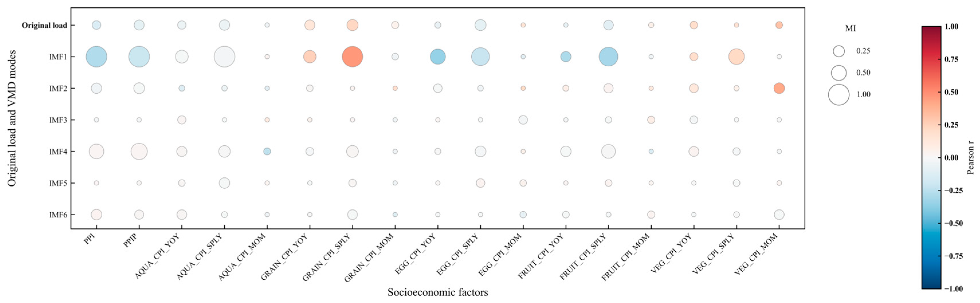
For the mutual-information analysis, MI was estimated using the k-nearest-neighbor estimator implemented in mutual_info_regression in scikit-learn, with k = 3 and random_state = 42.
All variables were independently rescaled to [0, 1] before estimation, and the same settings were applied to all external-variable–load-mode pairs. Pearson correlation describes linear association, whereas MI measures general statistical dependence. In the joint plots, the numerical labels represent Pearson coefficients and bubble size represents MI; MI was rescaled by the maximum value only for visualization. For the monthly Pearson association analysis, the circular moving-block bootstrap was performed using the 84 monthly observations from January 2015 to December 2021. The block length was set to 12 months to retain the annual dependence structure of the monthly series, and 4000 bootstrap samples were generated. The 2.5th and 97.5th percentiles were used to construct the 95% confidence intervals. Associations whose 95% confidence intervals excluded zero were retained in the block-bootstrap summary. The same bootstrap settings were applied to the meteorological and socioeconomic variable groups in both regions.