Condition-Aware Performance Health Index and Multi-Source Signal Mapping for Degradation Trend Identification in Hydropower Units

Abstract

Hydropower units often operate under complex conditions caused by water head change, guide-vane regulation, and load adjustment. These condition changes make it difficult to identify gradual performance degradation from monitoring signals alone. To solve this problem, this paper proposes a condition-aware performance health index construction and multi-source signal-mapping method for hydropower units. First, active power, guide-vane opening, and water head are used as the main operating variables. After data preprocessing and steady-state screening, water head is used as a prior constraint to divide the hydraulic boundary. FCM clustering is then used in each head layer to obtain different operating regions. Second, a high-quantile performance envelope is built in each operating region. The optimal active power is used as the performance benchmark, and the performance health index HI_perf is constructed by comparing actual power with optimal power. The results show that the proposed method can describe the performance deviation under comparable operating conditions. The smoothed daily HI_perf shows a degradation trend before maintenance and a recovery trend after maintenance. Finally, vibration and shaft-swing signals are mapped to HI_perf to construct the signal-based health index HI_sig. The mapping result shows good consistency between HI_sig and HI_perf, and shaft-swing features show stronger sensitivity than vibration features. The proposed framework focuses on daily-scale degradation trend identification using steady-state operating samples, while transient operating events are excluded from the current analysis. The proposed method provides a useful reference for degradation trend identification and health assessment of hydropower units under complex operating conditions.

1. Introduction

In pursuit of carbon peak and carbon neutrality, modern power grids are integrating a large number of wind and solar power resources. Hydropower stations no longer only provide baseload power generation; they now also act as the primary regulatory backbone in the multi-energy complementary system [1,2,3]. In particular, large-capacity conventional units and pumped-storage facilities play a crucial role. In this situation, hydropower units must frequently perform load tracking and rapid peak-shaving tasks. As a result, component wear, fatigue accumulation, and performance degradation may be further intensified [4,5]. Therefore, it is important to research degradation mechanisms and develop health management strategies for these units. This is essential to guarantee equipment safety and grid reliability.

Current studies on hydropower unit health assessment still have some limitations. Most methods focus on fault diagnosis or abnormal state recognition. They pay less attention to gradual performance degradation during non-fault operation. In addition, the effects of water head, guide-vane opening, and load regulation are often coupled with degradation-related changes. This makes it difficult to compare the health state under different operating conditions. Therefore, a health index with a clear performance benchmark is needed for degradation trend identification [6,7,8].

To address these limitations, this paper proposes a condition-aware performance health index construction and multi-source signal-mapping method for degradation trend identification of hydropower units. The proposed method establishes a condition-comparable performance benchmark through hydraulic-boundary-constrained operating condition partitioning and membership-weighted performance envelope modeling. On this basis, a performance health index is constructed to quantify degradation-related performance loss, and vibration and shaft-swing signals are further mapped to the index to verify the relationship between performance degradation and dynamic mechanical responses. The main contributions of this study are summarized as follows:

• A hydraulic-boundary-guided operating condition partitioning method is proposed. Water head is used as a prior constraint to separate the hydraulic boundary, and FCM clustering is further performed within each head layer to identify load-related operating regions. This strategy improves the comparability of samples under complex operating conditions and reduces the influence of condition mixing on health assessment.
• A condition-comparable performance health index ($H{I}_{perf}$) is developed. The high-performance output boundary under similar operating conditions is modeled by combining high-quantile regression with fuzzy membership weighting. The actual active power is then compared with the optimal power benchmark to construct a dimensionless health index, enabling degradation-related performance loss to be quantified across different water heads, guide-vane openings, and load levels.
• A multi-source signal-mapping method is introduced to characterize the dynamic response associated with performance degradation. The performance-side health index is first aggregated at the daily scale to obtain a degradation-oriented supervision target. Then, vibration and shaft-swing features are mapped to this target to construct a signal-based health indicator ($H{I}_{sig}$). This mapping establishes the relationship between performance loss and mechanical response characteristics, thereby providing additional evidence for degradation trend identification.

2. Related Work

2.1. Fault Diagnosis and Condition Monitoring

In recent years, with the rapid development of artificial intelligence, signal processing and information fusion, data-driven condition monitoring, and fault diagnosis of hydropower units have become one of the main research directions [9,10,11]. These studies are based on rich monitoring data, such as vibration, shaft-swing, sound, and pressure signals, and are usually combined with pattern recognition models. For example, Melani et al. [12] used a Petri net model to reveal the relationship between common guide-bearing faults and their possible causes. Chen et al. [13] analyzed the shaft orbit swing signal of a hydropower unit based on improved sample entropy, and extracted the features of typical fault states. Lan C et al. [14] proposed a diagnosis strategy based on turbine operating conditions and pressure pulsation, which improved the fault diagnosis effect under complex operating conditions. Dao F et al. [15] used wavelet transform and ensemble empirical mode decomposition to denoise the acoustic signal of a turbine runner under normal and sediment-laden flow conditions. Xu Li et al. [16] constructed a fault diagnosis model for hydropower units based on MCKD-MFFResNet, and enabled the diagnosis of shaft-system faults. With the increasing requirements for unit reliability and safety, monitoring and diagnosis methods based on a single information source have gradually been replaced by multi-source information methods. For example, Dao F et al. [17] proposed a BO-CNN-LSTM model based on Bayesian optimization, which showed good performance in the fault diagnosis of nonlinear acoustic-vibration signals of hydropower units.

Although these studies have improved the fault recognition and abnormal state detection capability of hydropower units, most of them are still fault-oriented. They mainly focus on identifying predefined fault types or abnormal operating states, while less attention is paid to the gradual degradation process during long-term non-fault operation. Therefore, it is necessary to further construct health indicators that can continuously characterize the degradation state of hydropower units.

2.2. Degradation Trend Assessment

In actual operation, faults of hydropower units do not occur frequently, but they may cause serious safety risks once they appear. To support early warning and predictive maintenance, degradation trend assessment has received increasing attention. In general, degradation trend prediction always includes two key parts. The first part is to construct a health index or a degradation evaluation index, which can convert monitoring data into a continuous state indicator. The second part is to build a trend prediction model which can be used to predict the future change of the index. Therefore, the quality of the health index and the accuracy of the prediction model are both important for the degradation assessment of hydropower units [18,19,20].

Existing studies usually construct health indicators from vibration signals, shaft-swing signals, pressure pulsation signals, or multi-source monitoring data. Shan et al. [21] used BPNN to build a health state model based on operating parameters and the Y-direction horizontal vibration of the lower bracket. The relative error between the healthy vibration value and the measured vibration value was defined as the degradation index. Then, an optimized KELM model was used for trend prediction. To capture the early degradation trend of hydropower units, Yunhe Wang et al. [22] proposed a comprehensive deterioration index based on weighted fusion of time-frequency features. An LSTM-based prediction model was built for the degradation state of hydropower units, and the effectiveness of the method was verified using actual operation data from a hydropower station.

In terms of unit state prediction, Wenlong Fu et al. [23] proposed a hybrid intelligent model for vibration signal trend prediction of hydropower units, and achieved high-accuracy prediction of vibration signal trends. Lei Xiong et al. [24] used a hybrid deep-learning structure combining one-dimensional CNN and LSTM to predict vibration signals. However, these studies were mainly conducted at the signal level, and could not directly describe the degradation trend of the unit. Li et al. [25] selected a low-dimensional feature subset related to the Y-direction shaft swing of the main thrust bearing from several operating parameters, including water head, active power, oil temperature, and excitation parameters. A DCGNN-based model was then developed to predict the shaft-swing signal. This study provided a signal-level method for unit-state prediction, but the predicted swing response could not be directly interpreted as unit degradation without further consideration of the operating-condition effects. Ke et al. [26] proposed an improved fuzzy comprehensive evaluation model by combining game-theory-based subjective and objective weighting with a Gaussian threshold method. A large amount of historical health data was used to dynamically define the operating boundary of the unit. This method improved the sensitivity and accuracy of comprehensive state assessments of hydropower units under complex operating conditions.

However, several problems still exist. First, many health indicators are built from signal features or statistical parameters, so their relationship with unit performance is not clear. Second, water head, guide-vane opening, and load regulation can affect active power, vibration, and shaft-swing signals at the same time. If these factors are not considered, normal condition changes may be confused with degradation [27,28]. Third, performance indicators and dynamic monitoring signals are often studied separately. The relationship between performance loss and monitoring signal responses still requires further study.

Overall, existing studies have provided useful methods for health index construction, degradation assessment, and trend prediction of hydropower units. However, many studies still focus on signal-side state description, while the condition-comparable characterization of gradual performance degradation remains insufficient. In addition, the coupling influence of water head, guide-vane opening, and load variation is not fully separated from degradation-related performance changes. The relationship between performance-side health indicators and multi-source signal responses also requires further study. These limitations motivate the development of a condition-aware performance health index and a multi-source signal-mapping framework in this study.

3. Methodology

3.1. Overview of the Proposed Framework

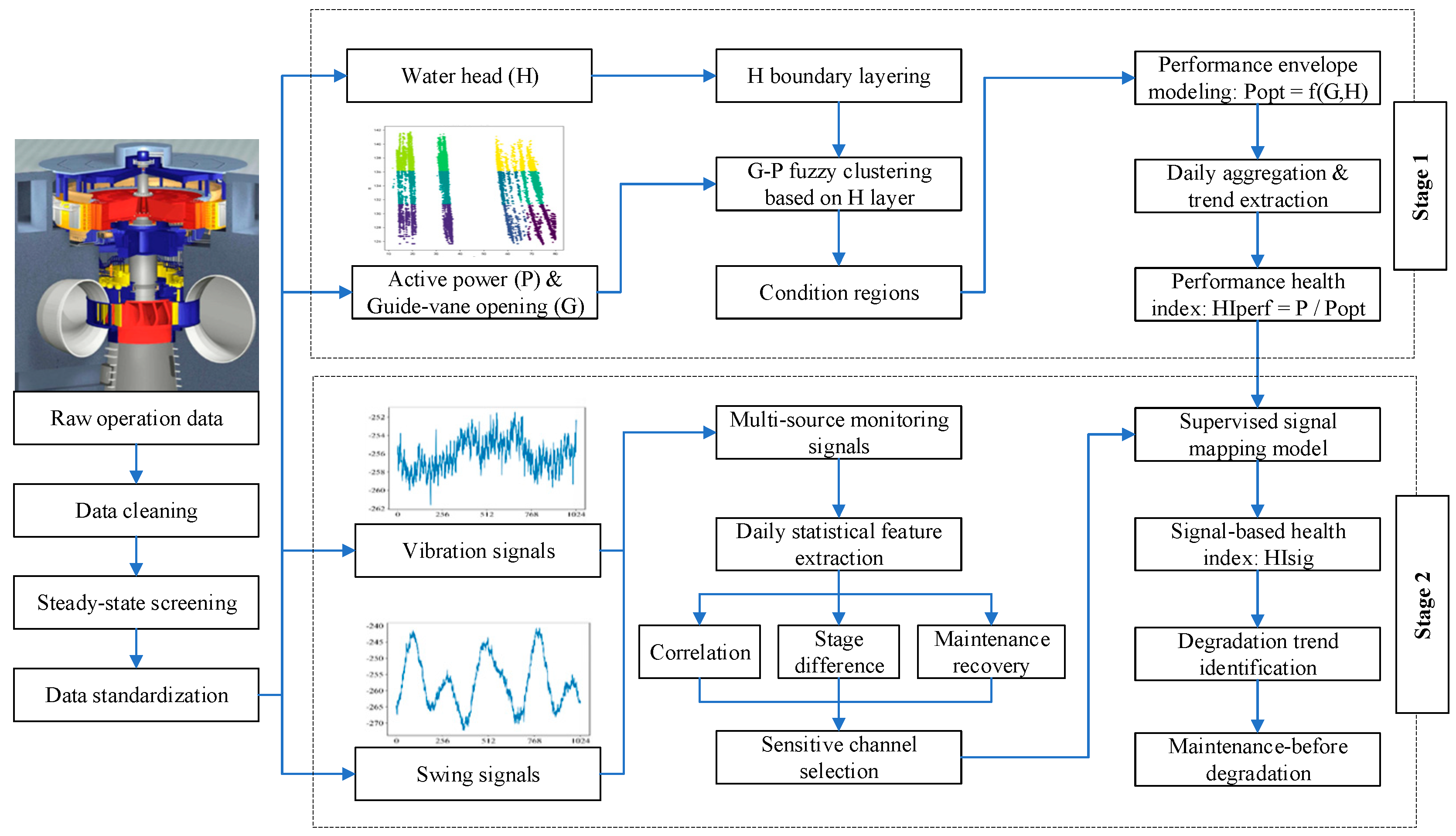
The proposed framework contains two main stages, as shown in Figure 1: condition-aware performance health index construction and multi-source signal health index mapping. The first stage constructs a performance health index from operating data, while the second stage maps multi-source monitoring signals to the constructed index to obtain a signal-based representation of the degradation trend.

In the first stage, active power $P$, guide-vane opening $G$, and water head $H$ are selected as the main operating variables. After data cleaning and steady-state screening, water head is used as a hydraulic boundary constraint to divide the samples into several water-head layers. Within each layer, guide-vane opening and active power are used for fuzzy clustering to identify load-related condition regions. For each condition region, a performance envelope model is established to estimate the optimal power output under different $G$ and $H$ values. The performance health index $H{I}_{perf}$ is then calculated by comparing the actual active power with the estimated optimal power, and daily trend extraction is further performed.

Performance maps obtained from index tests or IEC field efficiency tests provide authoritative references for unit performance under the tested configuration and conditions. However, such maps primarily reflect the unit configuration and condition during the test period. Long-term wear, aging, maintenance, rehabilitation, component replacement, or control-system adjustment may change the relationship among water head, guide-vane opening, and active power. Therefore, an earlier test-based map may not fully represent the current operational performance boundary or cover the operating domain recorded during long-term monitoring. In such cases, Stage 1 constructs an operational high-performance reference from long-term steady-state data. Because routine operating data are continuously recorded by existing monitoring systems, this data-driven scheme can provide a practical and readily implementable option for long-term performance evaluation.

In the second stage, vibration and shaft-swing signals are used to construct a signal-based health index. Daily statistical features are extracted from multiple channels, and sensitive channels are selected according to their correlation with $H{I}_{perf}$, stage differences and recovery behavior after maintenance. Then, a stable degradation-oriented target is obtained from $H{I}_{perf}$, and the selected vibration and shaft-swing features are used to construct the signal-based health index $H{I}_{sig}$. Finally, $H{I}_{perf}$ and $H{I}_{sig}$ are jointly analyzed to identify the degradation trend of the hydropower unit.

3.2. Data Preprocessing and Steady-State Screening

The original monitoring data contain missing records, abnormal values, and transient samples caused by load regulation, unit start-stop processes, and communication disturbances. Since the proposed performance health index is constructed from active power under comparable operating conditions, preprocessing mainly focuses on active power quality control and steady-state sample selection. Water head and guide-vane opening are used as condition variables, so they are not strongly modified to avoid changing the original operating-condition distribution.

First, samples with missing timestamps, active power, guide-vane opening, or water head are removed. The remaining samples are sorted by time. Then, a basic physical check is performed, and samples with non-positive active power are excluded. This ensures that the following performance modeling is based on valid power-generation records. To remove transient regulation processes, a steady-state screening strategy is further applied. For two adjacent samples at time $t_i$ and $t_{i-1}$, the time interval and operating-variable variations are calculated as

$$\Delta t_i=t_i-t_{i-1}$$

(1a)

$$\Delta P_i=\mid P\left(t_i\right)-P\left(t_{i-1}\right)\mid$$

(1b)

$$\Delta G_i=\mid G\left(t_i\right)-G\left(t_{i-1}\right)\mid$$

(1c)

$$\Delta H_i=\mid H\left(t_i\right)-H\left(t_{i-1}\right)\mid$$

(1d)

A sample is removed when the time interval or any operating-variable variation exceeds the corresponding threshold. This step removes discontinuous records, rapid load regulation samples, and obvious transient states. After steady-state screening, local spike detection is applied only to active power. A rolling median is calculated for active power, and the deviation from the rolling median is measured by median absolute deviation. Samples with abnormal deviations are regarded as local power spikes and removed. Before operating condition partitioning and performance envelope modeling, guide-vane opening and water head are further constrained by a normal G-H modeling domain. This step only removes unreasonable operating samples and does not modify the condition variables. Through these steps, valid steady-state samples are obtained for subsequent operating condition partitioning and performance envelope modeling. Non-steady-state samples were excluded because their rapid variations are mainly dominated by short-term hydraulic and mechanical transients and therefore do not provide a stable basis for performance evaluation. Their accumulated effects may still appear in subsequent steady-state performance changes. The proposed method uses daily aggregation of steady-state samples to identify degradation trends over several weeks to months, rather than individual transient events.

3.3. Condition-Aware Operating Region Partitioning

After data preprocessing and steady-state screening, the retained samples still contain different hydraulic boundaries and load levels. For hydropower units, water head directly affects the power output under the same guide-vane opening. If all samples are modeled together, the performance envelope may be affected by mixed operating conditions. Therefore, a condition-aware operating region partitioning strategy is introduced before performance envelope modeling.

In this study, water head is used as a prior constraint to define comparable hydraulic condition ranges. Here, the hydraulic boundary refers to the water-head range used to constrain the operating samples. Samples within the same head layer are considered to have relatively comparable hydraulic input conditions before load-state clustering. The steady-state samples are first divided into several water-head layers according to the distribution of H. In each water-head layer, the hydraulic boundary is relatively consistent, and the remaining differences are mainly related to load regulation.

Within each water-head layer, fuzzy C-means clustering is further performed using guide-vane opening $G$ and normalized active power $P_{norm}$ as clustering features. The use of $G$ reflects the guide-vane regulation state, while $P_{norm}$ represents the relative load level. Compared with hard clustering, FCM assigns a membership degree to each sample. This is useful for describing the soft transition among adjacent operating regions. The objective function of FCM is expressed as

$$J={\displaystyle \sum _{i=1}^{N_l}} {\displaystyle \sum _{c=1}^C}{u}_{ic}^m{\parallel z_i-v_c\parallel }^2$$

(2)

where $N_l$ is the number of samples in the current water-head layer, C is the number of clusters, $u_{ic}$ is the membership degree of sample i belonging to cluster c, m is the fuzzy weighting exponent, $z_i=[G_i,P_{norm,i}]$ is the input feature vector, and $v_c$ is the cluster center.

After the FCM iteration, each sample is assigned to its dominant operating region according to the maximum membership principle

$$r_i=arg \underset{c}{max} u_{ic}$$

(3)

The maximum membership degree is retained to describe the reliability of the region assignment. In addition, the fuzzy entropy of each sample is calculated as

$$E_i=-{\displaystyle \frac{1}{\mathit{ln}C}}{\displaystyle \sum _{c=1}^C}{u}_{ic}ln(u_{ic})$$

(4)

where $E_i$ reflects the uncertainty of the operating-region assignment. A smaller entropy indicates a clearer region attribution, while a larger entropy indicates that the sample may be located in a transition region.

Through this procedure, the operating space is divided by combining hydraulic boundary constraints and load-state fuzzy clustering. In the following performance envelope modeling, each operating region is modeled separately, and the membership information is used to adjust the sample weight. This strategy reduces the influence of condition mixing and provides a comparable data basis for health index construction.

3.4. Performance Envelope and Health Index Construction

After condition-aware operating region partitioning, a performance envelope model is established in each operating region to estimate the optimal active power under comparable operating conditions. For the $k$-th operating region, guide-vane opening $G$ and water head $H$ are used as input variables, and active power P is used as the output variable. The optimal power benchmark is defined as

$$P_{opt}=f_k(G,H)$$

(5)

where $P_{opt}$ denotes the estimated optimal active power, and $f_k(·)$ is the performance envelope model constructed in the $k$-th operating region.

A global quantile regression can also estimate an overall upper-performance surface by fitting all operating samples with a single model. In this method, explicit condition partitioning is introduced to establish locally comparable operating regions before envelope estimation. Water-head stratification constrains the hydraulic input range, while FCM separates overlapping load-related states and retains boundary information through fuzzy memberships. An independent envelope model $f_k$ is then trained in each region to capture the local relationship among water head, guide-vane opening, and active power. The same quantile level is used in all regions to maintain a consistent definition of the high-performance benchmark. This design is intended to reduce the influence of mixed operating distributions and uneven sample densities on local envelope construction.

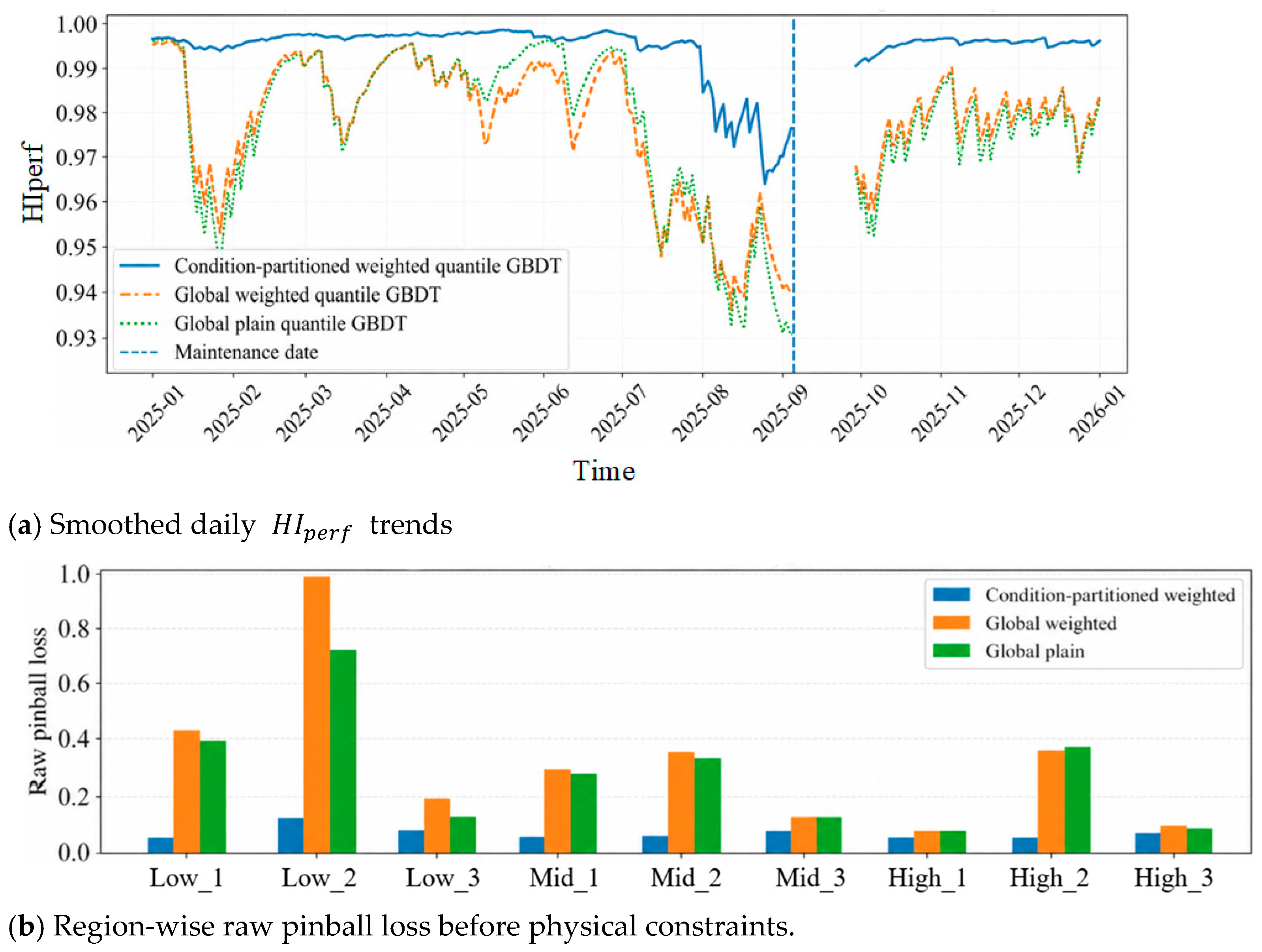
To further evaluate the effect of explicit condition partitioning, two global quantile GBDT baselines were constructed using the same modeling samples, input variables $G$ and $H$, quantile level $\alpha =0.92$, and GBDT settings as the proposed model. The global weighted baseline used q75 and q90 high-power weights calculated from all modeling samples, but fitted all samples using a single model without membership weighting. The global plain baseline used neither condition partitioning nor sample weighting. For all three models, the final daily $H{I}_{perf}$ trends were obtained using the same physical constraints, q35 aggregation, and EWM smoothing procedure. The raw pinball loss before physical constraints was calculated globally and within each fixed operating region.

Different from average regression models, the performance envelope aims to approximate the high-performance output boundary under similar operating conditions. Therefore, a high-quantile regression model is adopted. For a sample $i$, the quantile loss function is expressed as

$$L_{\alpha }(e_i)=\left\{\begin{array}{cc}\alpha e_i,& e_i\ge 0\\ (\alpha -1)e_i,& e_i<0\end{array}\right.$$

(6)

where $e_i=P_i-{\widehat{P}}_{opt,i}$, $\alpha$ is the quantile level, $P_i$ is the actual active power, and ${\widehat{P}}_{opt,i}$ is the predicted optimal power. A larger $\alpha$ makes the model pay more attention to high-output samples, so that the fitted result approaches the upper-performance boundary.

To improve the robustness of envelope modeling, sample weights are assigned according to the power level and fuzzy membership degree. The weight of sample $i$ is defined as

$$w_i=w_{p,i}{u}_i^{\beta }$$

(7)

where $w_{p,i}$ is the power-level weight, $u_i$ is the membership degree of the sample to its dominant operating region, and $\beta$ is the membership weighting exponent. In this way, high-performance samples with clear operating-region attribution contribute more to the envelope model. In this study, the performance envelope was implemented using a quantile Gradient Boosting Decision Tree model with 250 estimators, a maximum tree depth of 3, a learning rate of 0.05, and a minimum leaf sample number of 35.

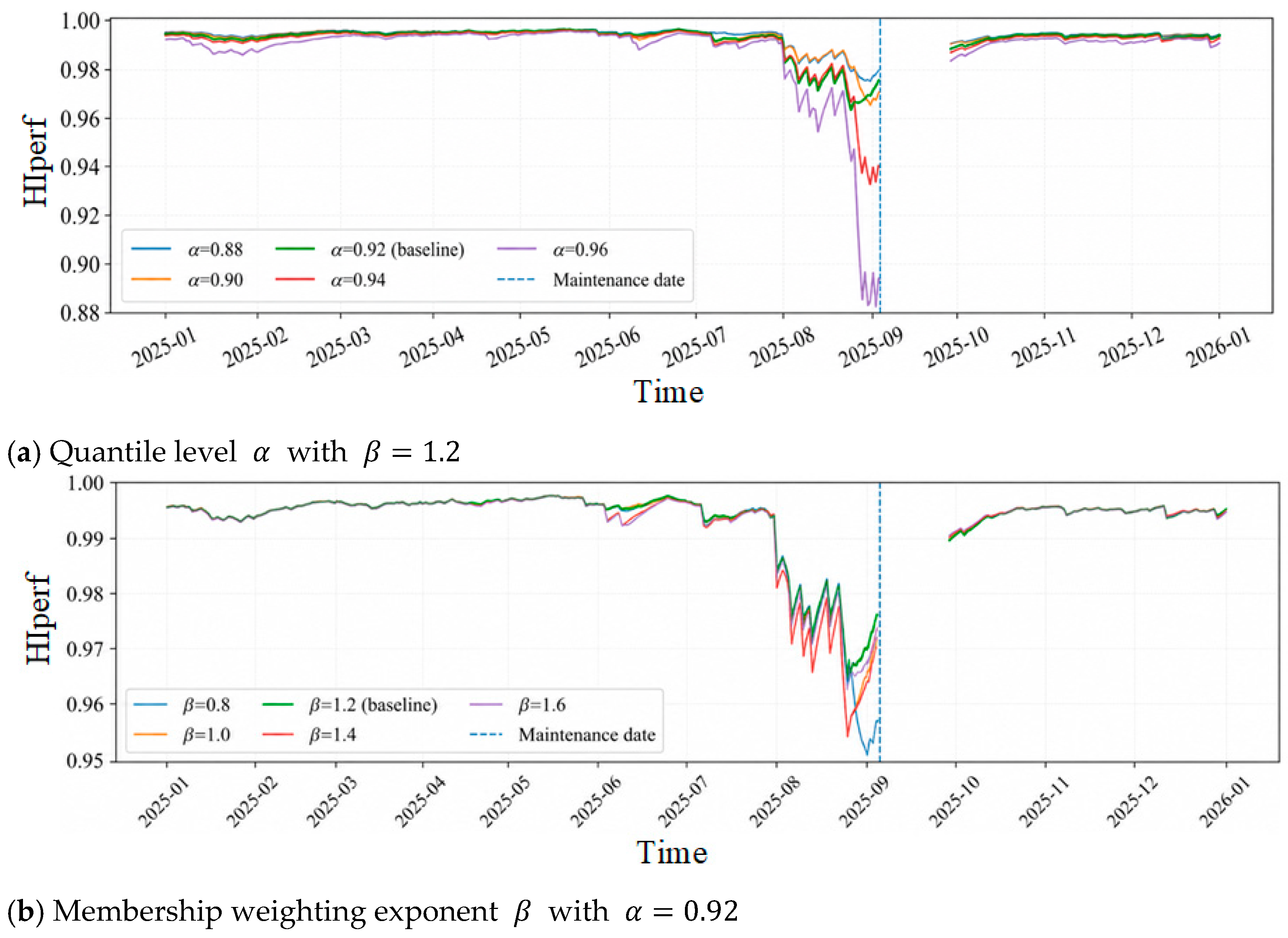
The quantile level $\alpha$ was set to 0.92, and the membership weighting exponent $\beta$ was set to 1.2. The same parameter settings were used for all operating regions to ensure consistent benchmark construction. To examine the influence of the two envelope parameters, a one-factor-at-a-time sensitivity analysis was conducted. With $\beta$ fixed at 1.2, $\alpha$ was set to 0.88, 0.90, 0.92, 0.94, and 0.96. With $\alpha$ fixed at 0.92, $\beta$ was set to 0.8, 1.0, 1.2, 1.4, and 1.6. The operating-region partitions, membership values, GBDT settings, physical constraints, daily q35 aggregation, and EWM smoothing were kept unchanged, and only the regional performance-envelope models were retrained.

Based on the estimated optimal power benchmark, the performance deviation is calculated as

$$\Delta P_i=P_{opt,i}-P_i$$

(8)

To reduce the influence of different load levels and obtain a dimensionless health indicator, the performance health index is defined as

$$H{I}_{perf,i}={\displaystyle \frac{P_i}{P_{opt,i}}}$$

(9)

When $H{I}_{perf}$ is close to 1, the actual power output is close to the optimal benchmark under similar operating conditions. A continuous decrease in $H{I}_{perf}$ indicates that the actual output deviates from the high-performance envelope, which may reflect performance degradation. For long-term trend analysis, the sample-level $H{I}_{perf}$ is further aggregated into a daily low-quantile series and smoothed within continuous valid segments.

3.5. Multi-Source Signal Mapping

After the performance health index $H{I}_{perf}$ is obtained, vibration and shaft-swing signals are further used to construct a signal-based health index. This stage does not aim to predict future degradation. Its purpose is to examine whether the dynamic monitoring signals contain information consistent with the performance-side health state.

Six vibration channels and six shaft-swing channels are selected as candidate signal channels. Since minute-level signals are easily affected by short-term disturbances and noise, daily statistical features are extracted from each channel, including the mean value, standard deviation, median value, 10% quantile, and 90% quantile. Meanwhile, the daily low-quantile value of $H{I}_{perf}$, namely $H{I}_{perf, q35}$, is used as the mapping target. Here, q35 denotes the 35% quantile of daily $H{I}_{perf}$. On the signal side, non-steady-state samples were excluded because vibration and shaft-swing responses under these conditions are strongly affected by short-term hydraulic and mechanical transients. Daily cleaning and aggregation were used to reduce event-driven fluctuations and capture persistent signal changes associated with long-term degradation. Therefore, $H{I}_{sig}$ is intended for daily-scale degradation trend mapping rather than individual transient-event analysis.

To reduce redundant information, sensitive channels are selected before mapping. The channel sensitivity is evaluated by considering the correlation with $H{I}_{perf,q35}$, the difference among different operating stages, and the recovery behavior after maintenance. The six channels with the highest comprehensive scores are retained. Five daily statistical features are extracted from each selected channel, including the mean, standard deviation, median, q10, and q90 values. Therefore, each daily sample is represented by a 30-dimensional signal feature vector.

A nonlinear mapping model is then established between the selected daily signal features and $H{I}_{perf,q35}$. XGBoost is used as the main mapping model, while GBDT and Random Forest are used for comparison. The mapped output is defined as

$$H{I}_{sig,d}=F\left(x_d\right)$$

(10)

where $x_d$ is the 30-dimensional signal feature vector on day $d$, $F\left(\cdot \right)$ denotes the nonlinear mapping model, and $H{I}_{sig,d}$ is the signal-based health index. Therefore, the model performs a day-wise many-to-one feature mapping from the daily signal features to one daily health-index value, rather than multi-step future forecasting.

The full-sample mapping analysis is first used to evaluate the consistency between the signal-based index and the performance-side health index. To further examine the mapping ability on unseen samples, repeated stage-stratified independent testing is conducted. In each run, 70% of the daily samples are randomly selected for training and the remaining 30% are used as an independent test set. The split is stratified according to the normal, degradation-related, and post-maintenance stages, so that all three stages are represented in both sets. Sensitive-channel ranking, missing-value imputation, stage-balanced sample weighting, and model training are performed using the training set only. The procedure is repeated 20 times using different random seeds.

To reduce overfitting on the relatively small daily training sets, a fixed regularized XGBoost configuration is used in all independent-test runs, including 500 estimators, a maximum tree depth of 2, a learning rate of 0.02, a subsample ratio of 0.80, a column-sampling ratio of 0.75, a minimum child weight of 5, an L1 regularization coefficient of 0.10, and an L2 regularization coefficient of 10.0. The representative XGBoost result is selected as the run whose MAE is closest to the median MAE over the 20 runs, rather than the run with the best test result.

4. Results and Discussion

4.1. Data Description

The proposed method is validated using the annual operating data of a Francis turbine-generator unit from a hydropower station in the Yellow River basin, China. The rated power of the studied unit is 320 MW, and the monitoring data cover the whole year of 2025 with a sampling interval of one minute. For the investigated unit, a complete and current state-matched test-based performance map covering the monitored operating domain was not available for this study. Therefore, Stage 1 was used to construct an operational high-performance reference from long-term steady-state data. The selected variables include operating variables and multi-source monitoring signals.

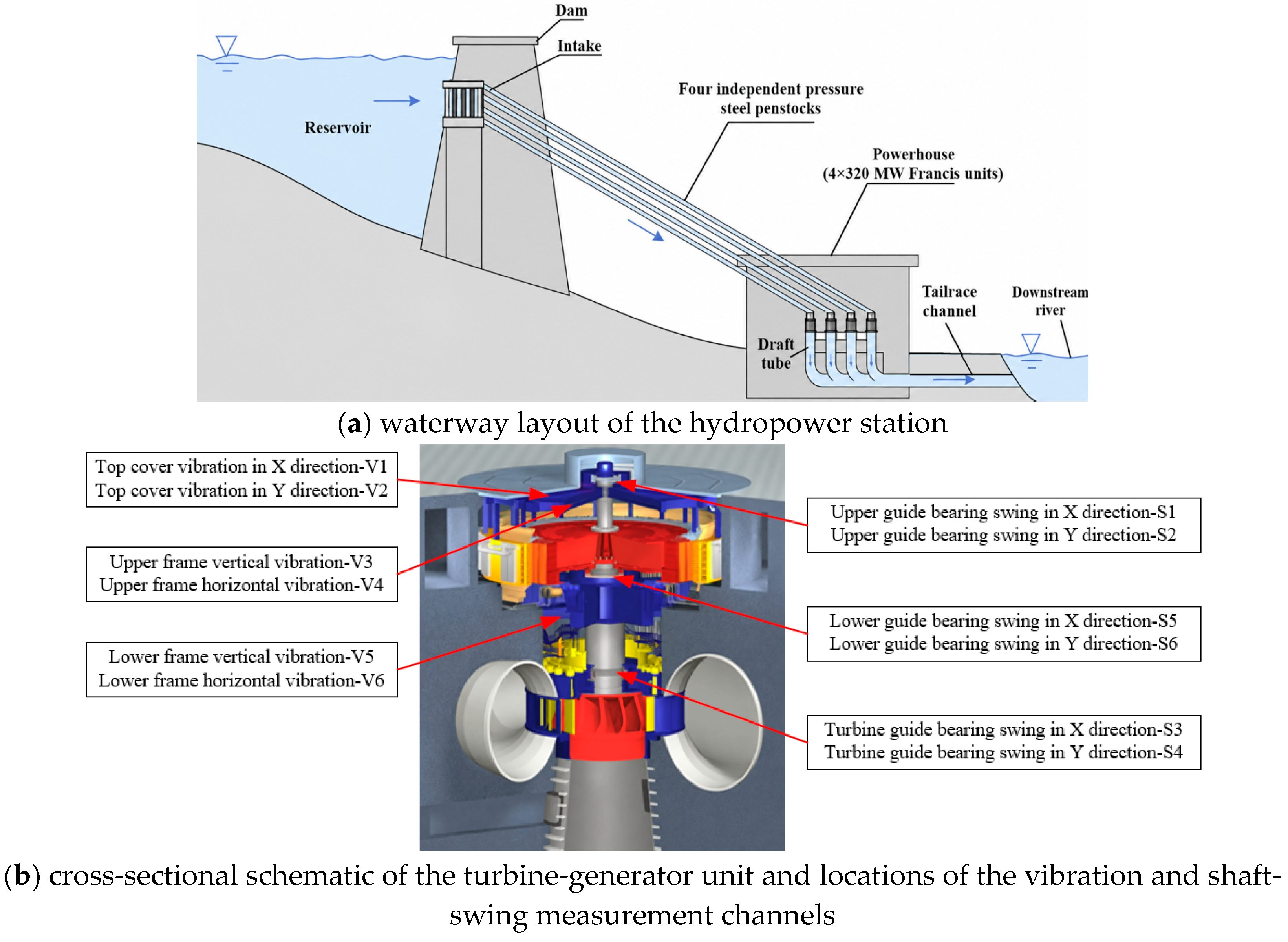
The operating variables include active power P, water head H, and guide-vane opening G, which are used for operating condition partitioning, performance envelope modeling, and $H{I}_{perf}$ construction. The multi-source monitoring signals include six vibration channels, V1 to V6, and six shaft-swing channels, S1 to S6, which are used for signal-based health index mapping. The selected variables are listed in

Table 1. Description of the selected monitoring variables.

Data Type	Signal Description	Symbol
Operating variable	Active power	P
	Water head	H
	Guide-vane opening	G
Vibration signal	Top-cover vibration in X-direction	V1
	Top-cover vibration in Y-direction	V2
	Upper-frame vertical vibration	V3
	Upper-frame horizontal vibration	V4
	Lower-frame vertical vibration	V5
	Lower-frame horizontal vibration	V6
Shaft-swing signal	Upper guide-bearing swing in X-direction	S1
	Upper guide-bearing swing in Y-direction	S2
	Turbine guide-bearing swing in X-direction	S3
	Turbine guide-bearing swing in Y-direction	S4
	Lower guide-bearing swing in X-direction	S5
	Lower guide-bearing swing in Y-direction	S6

. The twelve channels are selected mechanical dynamic monitoring channels rather than the complete monitoring installation. Vibration and shaft swing were selected because of their fast responses, high temporal resolution, and sensitivity to structural and shaft-system changes. Pressure pulsation, bearing temperatures, seal flows, and other process variables may provide additional information and will be considered in future multi-source mapping studies.

Figure 2a presents a simplified waterway layout of the studied hydropower station, while Figure 2b presents a cross-sectional schematic of the turbine-generator unit. The waterway schematic illustrates the main flow path through the hydraulic conveyance system and the turbine. The cross-sectional schematic shows the relative locations of the vibration and shaft-swing measurement channels. Figure 2 is a simplified representation intended to show the waterway configuration and relative sensor locations.

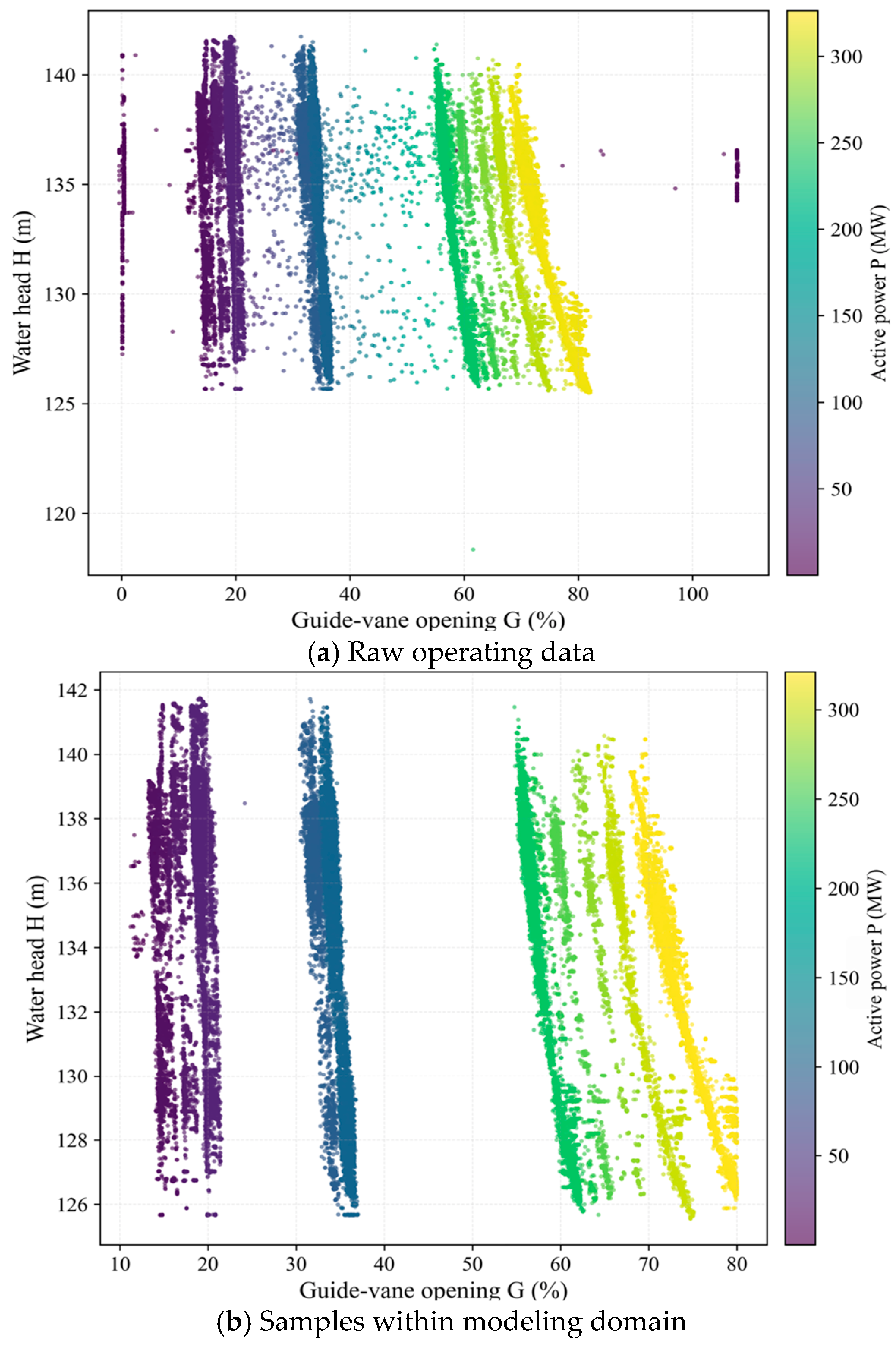
To analyze the operating-condition distribution of the unit, the original G-H-P samples are visualized in three-dimensional space and projected planes, as shown in Figure 3. The samples present obvious multi-layer and band-like distributions, indicating that the unit operates under multiple load levels and hydraulic conditions. In the G-H projection, the samples are concentrated in several guide-vane opening regions, while water head still varies within each opening range. This indicates that active power is strongly coupled with both water head and guide-vane opening. In addition, some scattered samples and local abnormal points can be observed, which may be related to transient regulation processes, measurement disturbances, or communication errors. Therefore, data preprocessing, steady-state screening, and condition-aware operating region partitioning are necessary before performance health index construction.

4.2. Data Preprocessing and Operating Condition Partitioning

To construct a reliable performance envelope under comparable operating conditions, the raw annual operating data were first preprocessed to obtain effective steady-state samples. The preprocessing procedure mainly included data validity checking, basic physical sanity checking, steady-state screening, and local active-power spike filtering. In this process, invalid records, sharp fluctuation samples, and isolated power disturbances were removed, while guide-vane opening and water head were not excessively modified, so as to preserve the original operating-condition distribution.

A total of 488,448 valid samples with available P, G, and H were obtained from the raw records. After steady-state screening and local spike filtering, 460,594 effective samples were retained, corresponding to a preprocessing retention ratio of 94.30%. Then, the samples were constrained to the normal G-H modeling domain before condition partitioning and performance envelope modeling. Finally, 431,183 samples were retained for subsequent analysis. This indicates that most valid records were preserved, while unstable and unsuitable samples were excluded.

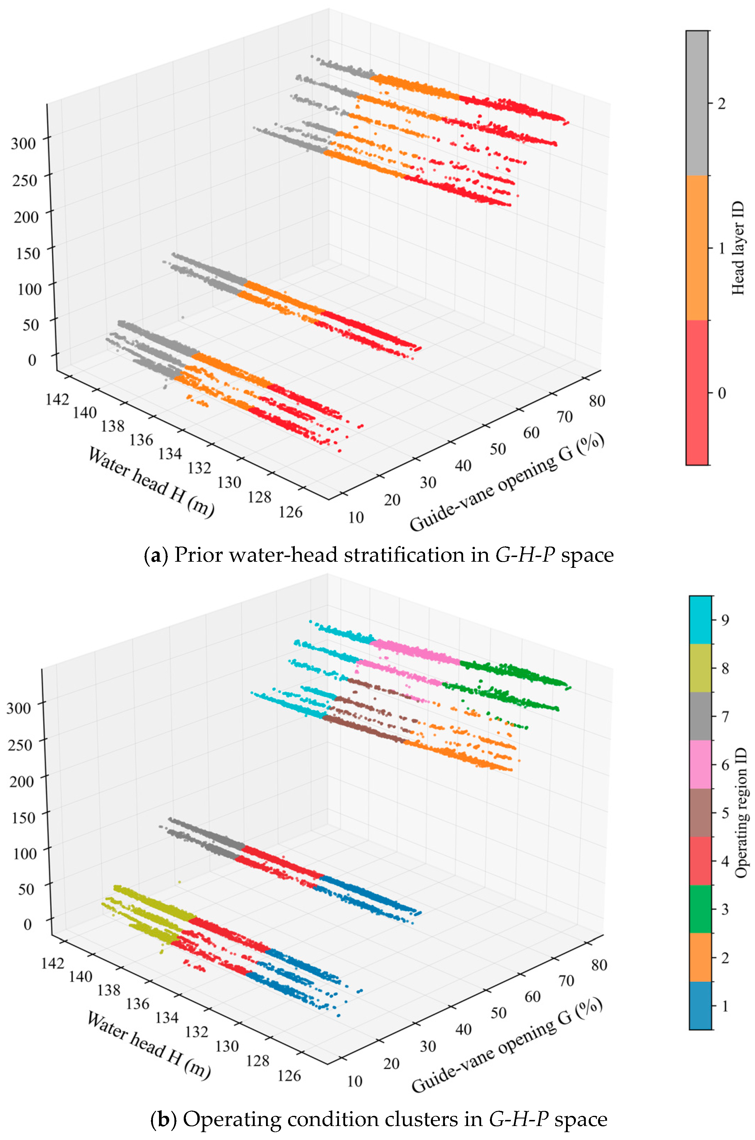
Based on the retained samples, water head was first introduced as a prior hydraulic boundary to divide the operating data into three head layers. The low-head, medium-head, and high-head layers contained 143,728, 143,736, and 143,719 samples, respectively. The H ranges of the three layers were 125.53 to 131.51 m, 131.51 to 136.37 m, and 136.37 to 141.76 m, respectively. The nearly balanced sample sizes indicate that the stratification provides a sufficient data basis for subsequent layer-wise clustering. Meanwhile, the guide-vane opening and active power ranges varied among different head layers, confirming that the operating boundary of the unit is strongly affected by water head.

Within each water-head layer, FCM clustering was further performed using guide-vane opening and normalized active power to identify load-regulation patterns. Finally, nine operating regions were constructed. The detailed partitioning results are summarized in

Table 2. Operating regions obtained by prior water-head-guided fuzzy clustering.

Zone	Samples	H Range (m)	G Range (%)	P Range (MW)	Mean Membership	Mean Entropy
Low_1	58,471	125.59–131.51	13.76–37.01	3.07–102.05	0.9101	0.3138
Low_2	16,356	125.53–131.51	56.97–68.83	234.93–281.08	0.9599	0.1027
Low_3	68,901	125.55–131.51	68.00–80.00	278.18–321.24	0.9651	0.1129
Mid_1	49,746	131.51–136.37	10.93–35.77	0.01–103.78	0.9182	0.2975
Mid_2	25,534	131.51–136.37	55.59–65.00	234.31–280.89	0.9464	0.1142
Mid_3	68,456	131.51–136.37	64.33–75.12	278.44–321.25	0.9741	0.0760
High_1	50,343	136.37–141.76	30.22–35.18	87.31–103.98	0.9952	0.0269
High_2	55,503	136.37–141.75	11.14–24.18	0.01–54.09	0.9871	0.0625
High_3	37,873	136.37–141.47	54.77–72.61	235.41–320.99	0.9452	0.2173

. As shown in the table, the obtained regions cover different combinations of water head, guide-vane opening, and active power level, which indicates that the proposed partitioning method can separate hydraulic boundary and load-regulation effects.

As shown in Table 2, the mean maximum membership values of all regions are higher than 0.91, indicating that most samples have clear dominant operating-region attributes. The mean fuzzy entropy values are generally low, especially in the high-head, low-load, and medium-load regions. This further shows that the fuzzy clustering results are stable. Compared with hard partitioning, the FCM-based strategy can retain the soft transition information between adjacent operating states and is therefore more suitable for hydropower units with continuous load regulation.

Figure 4 shows the operating condition clusters obtained by the prior water-head-guided fuzzy clustering strategy in the G-H-P space. The samples present clear layered and banded distributions. Under the constraint of water head, the operating data are first separated into different hydraulic boundary regions. Within each head layer, different load levels are further distinguished according to guide-vane opening and active power. High-load regions are mainly distributed at larger guide-vane openings and higher active power levels, while low-load regions are concentrated at smaller openings and lower power outputs. These results indicate that the proposed strategy can separate the effects of hydraulic boundary and load regulation, thereby providing condition-comparable samples for subsequent zone-wise performance envelope modeling.

Although normalized power is useful for describing the relative load level, it was not used to replace water head as the sole prior boundary. Active power is affected by water head, discharge, unit efficiency, and health condition. Therefore, a decrease in power may be caused by either a load change or performance degradation. Moreover, active power is used as the output of the performance envelope and the numerator of $H{I}_{\mathrm{p}\mathrm{e}\mathrm{r}\mathrm{f}}$. Using it again as the sole condition boundary may increase the coupling between condition partitioning and performance evaluation. In addition, the same normalized power may correspond to different combinations of water head, discharge, and guide-vane opening, which may produce different vibration and shaft-swing responses. Therefore, water head was retained as the prior hydraulic boundary, while normalized power and guide-vane opening were jointly used within each head layer to describe the load and control states.

4.3. Performance Envelope Modeling and Degradation Trend

After operating condition partitioning, the performance envelope was modeled separately in each operating region. For each region, guide-vane opening G and water head H were used as input variables, and active power P was used as the output variable. Different from ordinary mean regression, the purpose of the envelope model was to estimate the high-performance output boundary under comparable operating conditions. Therefore, the estimated optimal power $P_{opt}$ was used as a condition-comparable benchmark for evaluating the performance deviation of the unit.

The fitting results of different operating regions are summarized in

Table 3. Zone-wise performance envelope fitting results.

Zone	Samples	R2	MAE (MW)	P Range (MW)
Low_1	58,471	0.9995	0.4677	3.07–102.05
Low_2	16,356	0.9549	1.1582	234.93–281.08
Low_3	68,901	0.9427	0.9076	278.18–321.24
Mid_1	49,746	0.9985	0.5434	0.01–103.78
Mid_2	25,534	0.9909	0.5238	234.31–280.89
Mid_3	68,456	0.9650	0.8720	278.44–321.25
High_1	50,343	0.9334	0.4607	87.31–103.98
High_2	55,503	0.9810	0.4489	0.01–54.09
High_3	37,873	0.9982	0.8111	235.41–320.99

. The R² values of all operating regions are higher than 0.93, and most regions are higher than 0.95. The MAE values are lower than 1.16 MW in all regions. Considering that the rated power of the unit is 320 MW, the fitting errors are relatively small. This indicates that the zone-wise envelope models can provide a reasonable approximation of the power-output boundary within comparable operating regions.

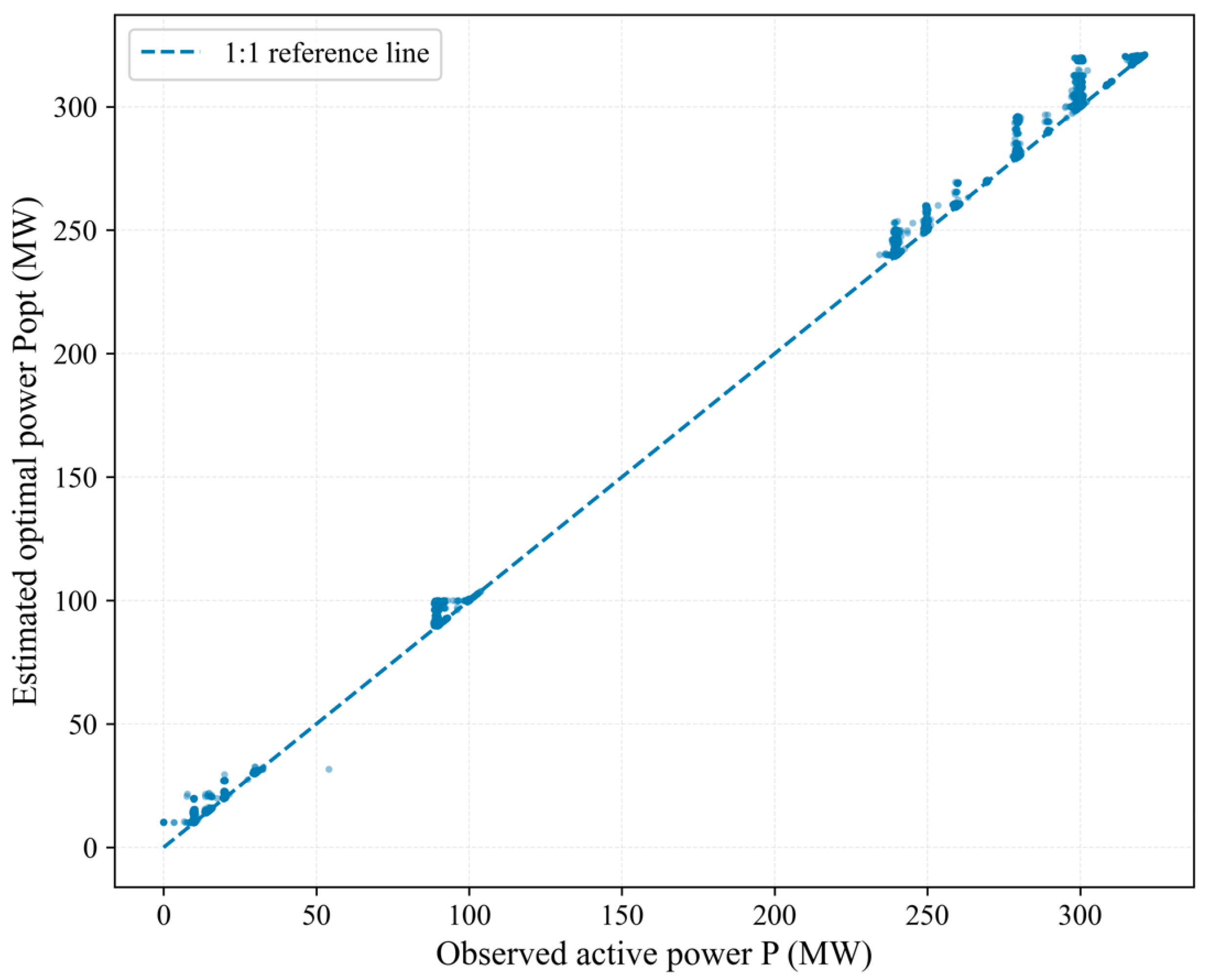
Figure 5 shows the relationship between the observed active power P and the estimated optimal power $P_{opt}$. The samples are distributed close to the 1:1 reference line over different power levels, indicating that the estimated benchmark is consistent with the actual operating range of the unit. At the same time, $P_{opt}$ is generally located near or slightly above the observed power, which is consistent with the definition of a performance envelope. This result shows that the constructed envelope can provide a reasonable optimal power reference for health index calculation.

Based on the estimated optimal power benchmark, the performance health index $H{I}_{perf}$ was calculated as the ratio of actual active power to optimal active power. After stability control, 430,154 valid minute-level HI samples were retained from 431,183 samples, with a retention ratio of 99.76%. This indicates that the constructed $H{I}_{perf}$ values were generally stable, and only a very small proportion of abnormal HI points were excluded.

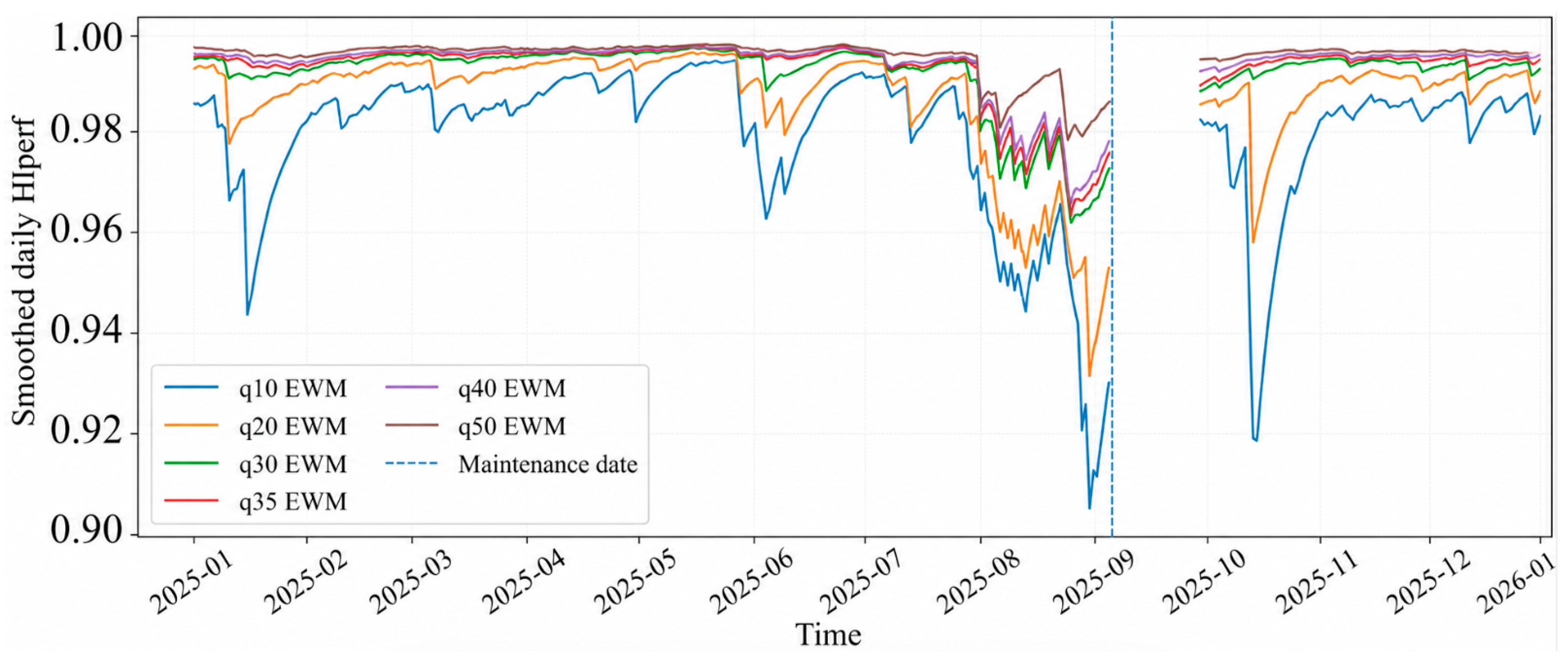
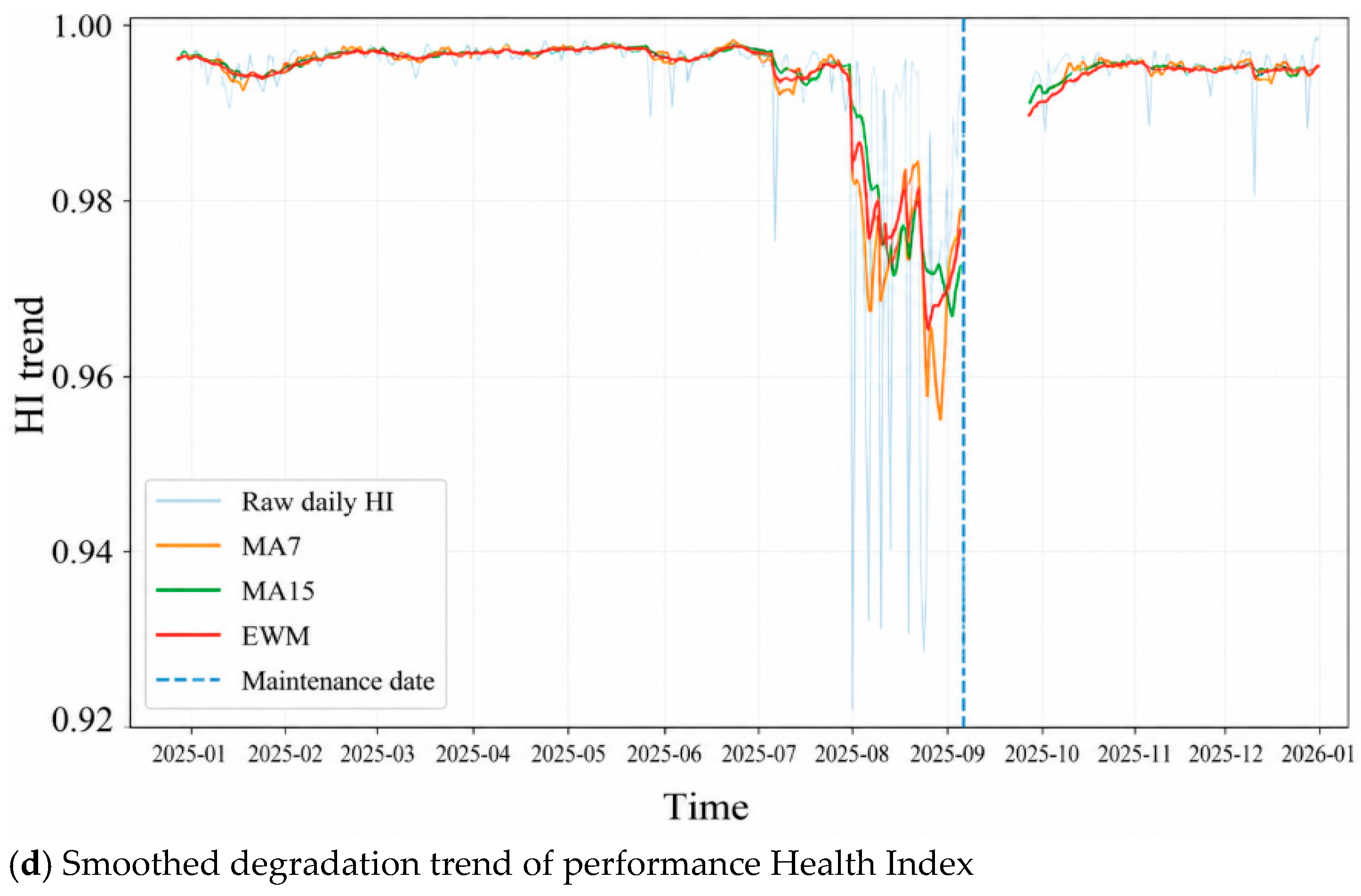
To examine the influence of daily quantile selection on trend extraction, several quantile levels were compared, as shown in Figure 6. The smoothed HI curves under different quantile levels show generally consistent variation patterns. The q10 and q20 curves are more sensitive to short-term fluctuations, while the q50 curve is relatively smooth but less sensitive to performance decline. In contrast, q30, q35, and q40 show similar degradation and recovery trends. Therefore, q35 was selected as a representative low-quantile setting for daily $H{I}_{perf}$ aggregation.

Figure 7 compares the smoothed daily $H{I}_{perf}$ trends under different envelope parameter settings. For the non-baseline $\alpha$ settings, the Pearson and Spearman correlations with the baseline trend ranged from 0.8849 to 0.9835 and from 0.9236 to 0.9933, respectively, with an MAE of 0.0012 to 0.0048. A lower $\alpha$ produced a looser benchmark and weakened the observed degradation, while a higher $\alpha$ enlarged the pre-maintenance decrease. In particular, $\alpha =0.96$ showed greater sensitivity to upper-tail samples. Therefore, $\alpha =0.92$ was retained as a balanced setting that preserved the degradation and recovery pattern without excessive amplification.

For $\beta$, the Pearson and Spearman correlations ranged from 0.9518 to 0.9977 and from 0.9623 to 0.9969, respectively, and the MAE was only 0.0003 to 0.0007. The curves were highly consistent, indicating low sensitivity to $\beta$. A smaller $\beta$ weakens membership discrimination, whereas a larger value suppresses boundary samples more strongly. Thus, $\beta =1.2$ was retained as a moderate weighting setting. Overall, the main degradation and recovery conclusions remained stable in the tested parameter ranges.

Figure 8 compares the proposed condition-partitioned model with two global quantile GBDT baselines. The global weighted model retained the q75 and q90 high-power sample weights but fitted all samples using a single envelope model. The global plain model used neither condition partitioning nor sample weighting. All three models used the same samples, input variables, quantile level, GBDT settings, physical constraints, and daily trend-extraction procedure.

Pinball loss is the standard loss function for quantile regression. A lower value indicates that the estimated upper-performance envelope is closer to the target quantile. The region-wise pinball losses in Figure 8b were calculated from the raw envelope predictions before physical constraints. Therefore, they directly reflect the original fitting ability of each model. The proposed model achieved an overall pinball loss of 0.0623, compared with 0.2632 for the global weighted model and 0.2373 for the global plain model. Its mean region-wise pinball loss was 0.0663, compared with 0.3224 and 0.2793 for the two global models. The worst region-wise pinball loss was reduced from 0.9933 and 0.7190 to 0.1254. The envelope MAE was also reduced from 3.134 MW and 2.795 MW to 0.677 MW. Moreover, the proposed model obtained the lowest pinball loss in all nine operating regions.

As shown in Figure 8a, both global models identified the general pre-maintenance decrease. However, their daily $H{I}_{perf}$ trends showed larger fluctuations during the earlier normal period and remained at lower levels after maintenance. The similar trends of the two global models indicate that global high-power sample weighting alone cannot effectively reduce the influence of mixed operating conditions. In contrast, the condition-partitioned model provided a more stable operational reference and a clearer degradation–recovery pattern. These results show that explicit partitioning improves local envelope adaptability and reduces interference from mixed operating distributions.

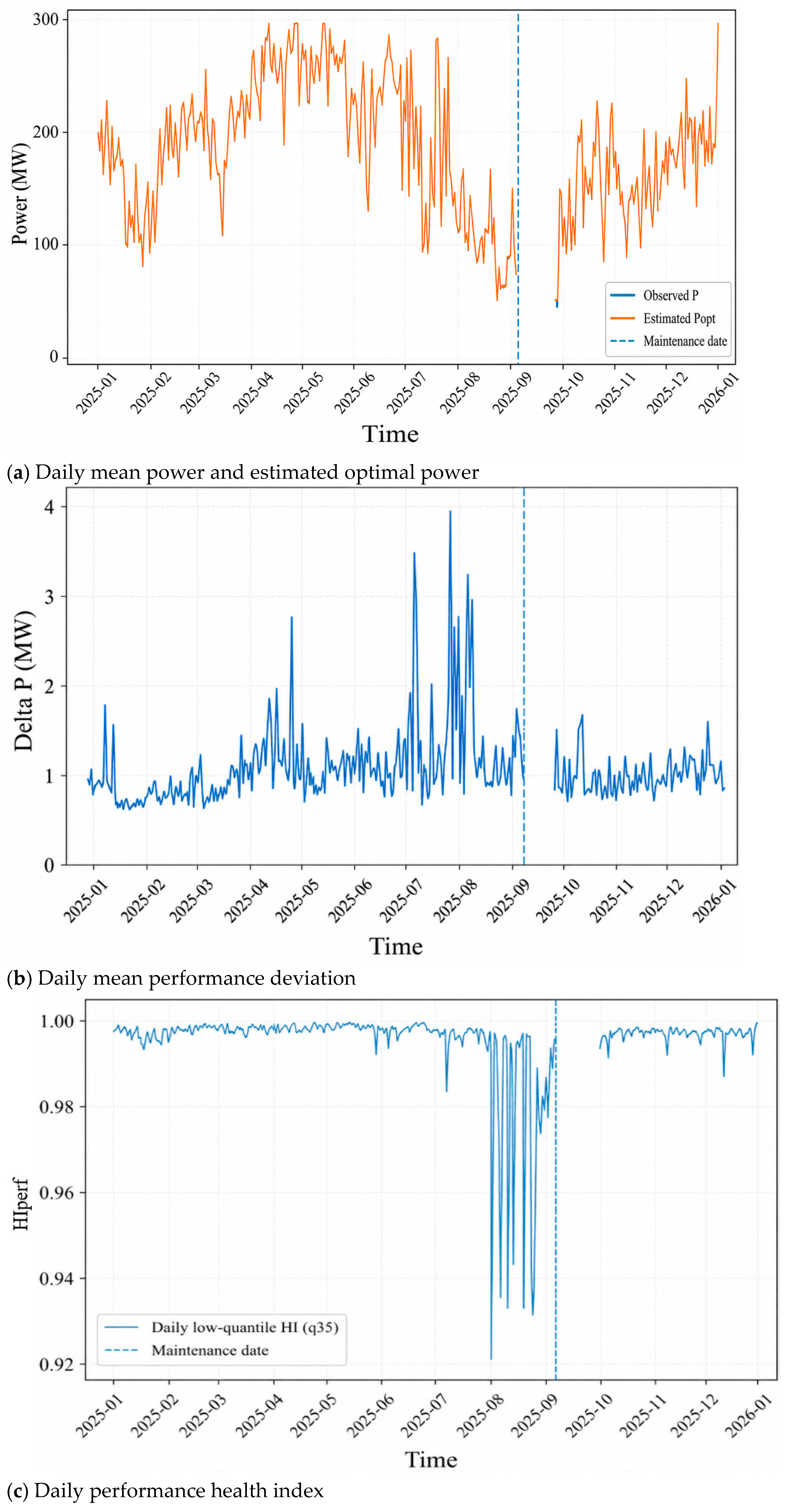
Figure 9 shows the performance degradation trend based on $P_{opt}$, $\Delta P$ and $H{I}_{perf}$. The dashed vertical line indicates the beginning of the maintenance period, 5 September 2025. The daily mean values of $P$ and $P_{opt}$ show similar variation patterns, indicating that the estimated optimal power benchmark can follow the long-term load changes of the unit. From January to June, the smoothed $H{I}_{perf}$ remains close to 1.0, suggesting that the actual power output is close to the performance envelope under comparable operating conditions. Around July and August, $\Delta P$ increases obviously, while the smoothed $H{I}_{perf}$ decreases synchronously. This indicates that the actual output gradually deviates from the condition-comparable performance envelope during this period.

After the maintenance period, the smoothed $H{I}_{perf}$ returns to a higher level and remains relatively stable from October to December, while $\Delta P$ also decreases. A total of 342 valid daily HI values were obtained, with a mean value of 0.9932, a median value of 0.9959, and a minimum value of 0.9124. The minimum value mainly corresponds to the short-term fluctuation period before maintenance. Therefore, the degradation trend is mainly interpreted from the smoothed HI curve rather than from isolated daily low-quantile points. These results indicate that $H{I}_{perf}$, together with $\Delta P$, can reveal the performance degradation tendency before maintenance and the recovery behavior after maintenance.

Overall, the proposed performance envelope provides a condition-comparable optimal power benchmark. The derived $H{I}_{perf}$ can quantify the deviation between actual power and optimal power, and the daily $H{I}_{perf,q35}$ trend can reveal the long-term degradation and recovery trend of the hydropower unit.

4.4. Signal-Mapping Results

After the performance health index was obtained, vibration and shaft-swing signals were further used to construct the signal-based health index $H{I}_{sig}$. The daily low-quantile performance health index $H{I}_{perf,q35}$ was used as the mapping target. This stage was used to evaluate the consistency between the performance-side health state and the dynamic monitoring signals, rather than to predict the future degradation state.

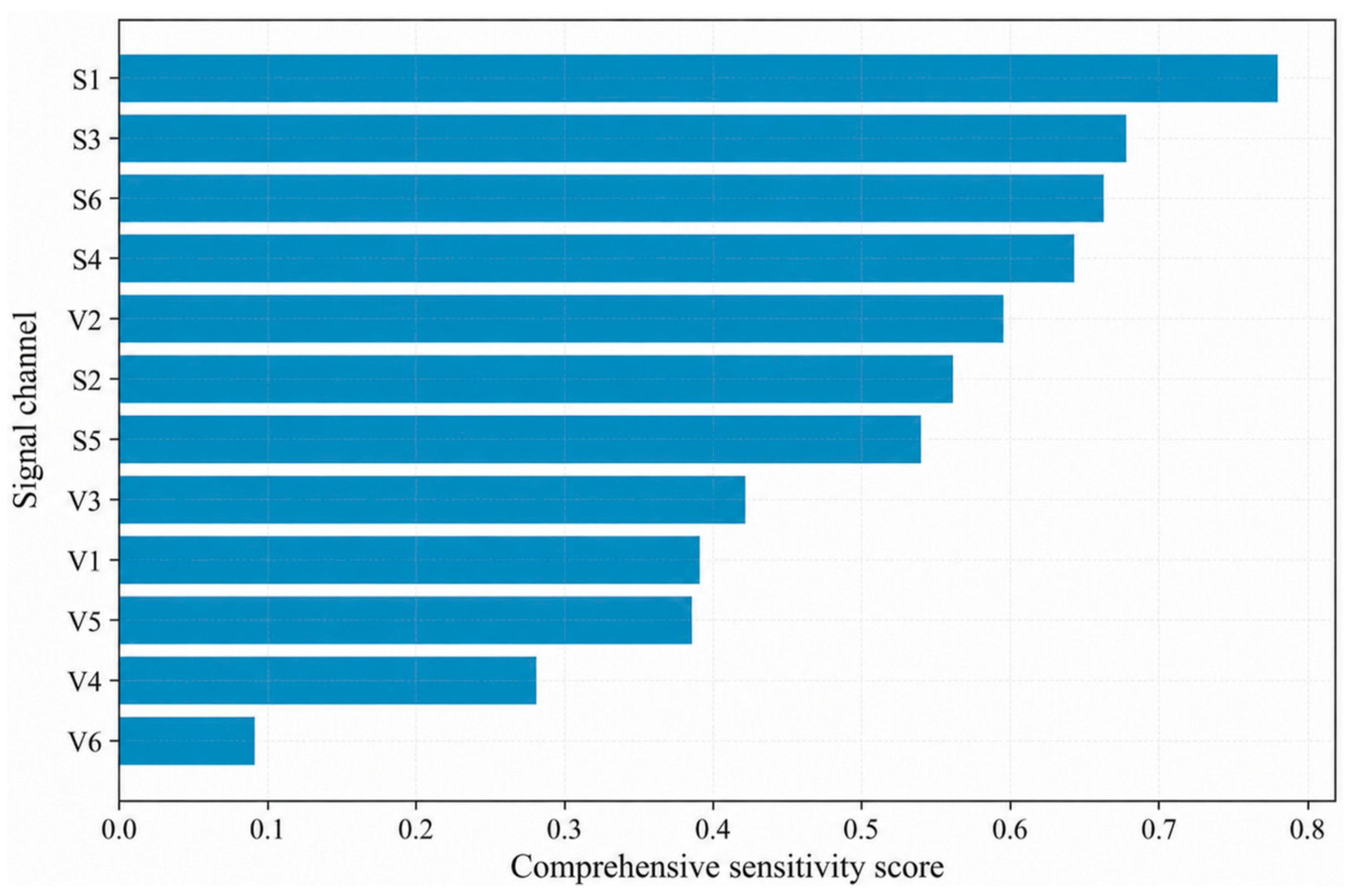
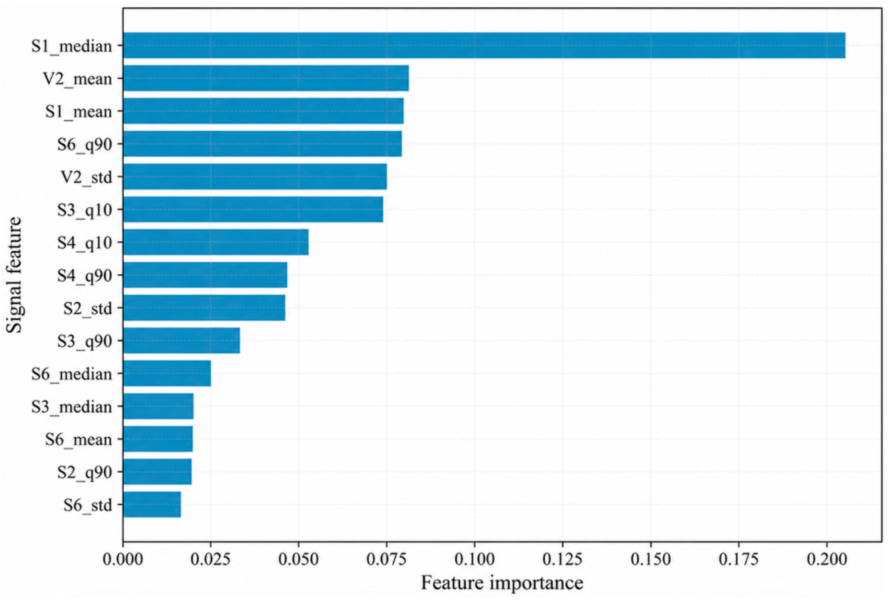
First, sensitive signal channels were selected from the candidate vibration and shaft-swing channels. The comprehensive sensitivity score was calculated by considering correlation, stage difference, and maintenance recovery. As shown in Figure 10, the top six sensitive channels were S1, S3, S6, S4, V2, and S2. Most of them were shaft-swing channels. This indicates that shaft-swing signals are more sensitive to the performance health change of the studied unit. The selected channels were then used to extract daily statistical features for signal mapping.

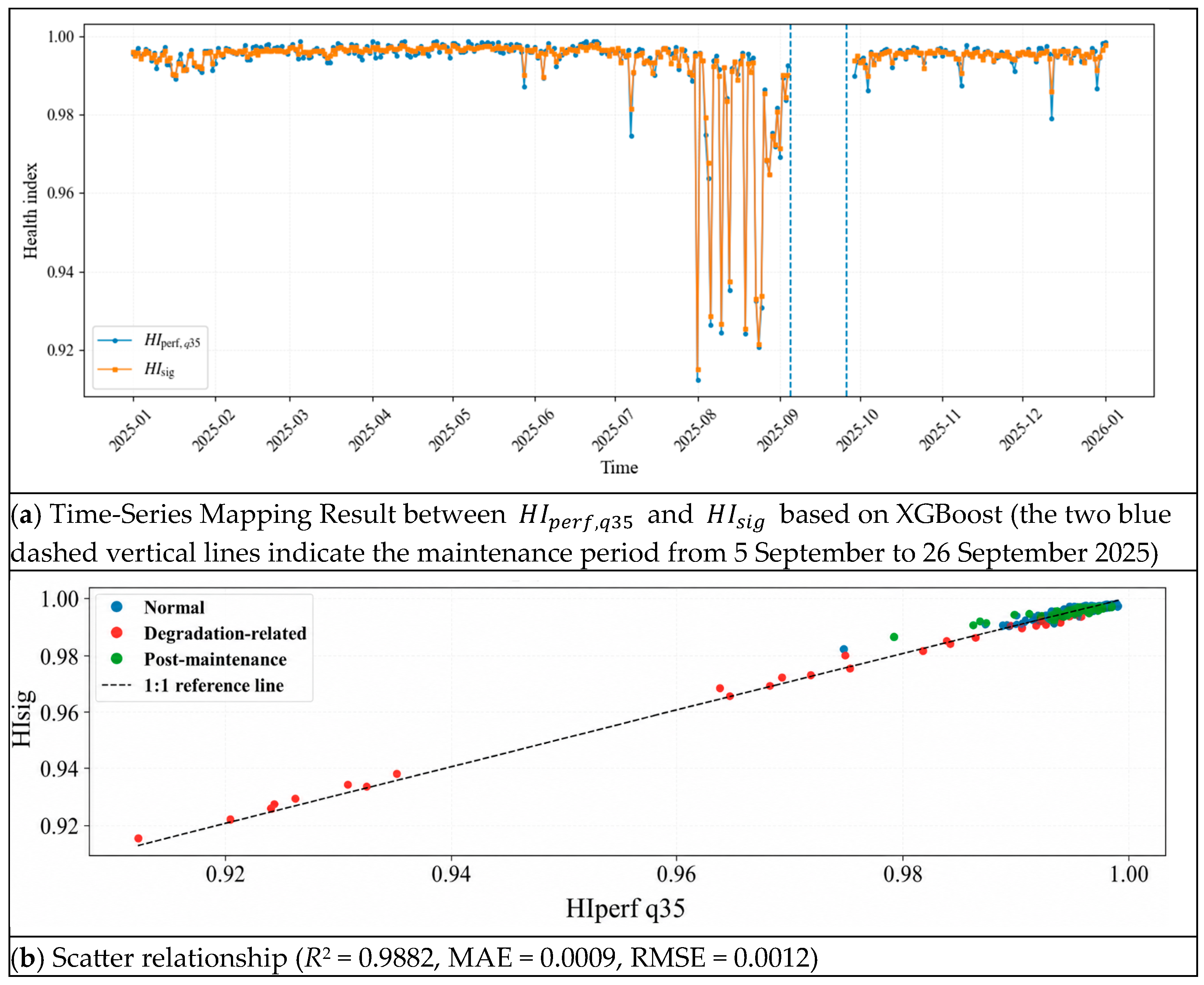
To evaluate the full-sample mapping consistency, XGBoost, GBDT, and Random Forest were compared. As shown in

Table 4. Full-sample mapping consistency comparison of different signal-mapping models.

Model	R2	MAE	RMSE
XGBoost	0.9882	0.0009	0.0012
GBDT	0.9852	0.0009	0.0014
Random Forest	0.8519	0.0017	0.0044

, XGBoost obtained the best full-sample mapping result, with an $R^2$ of 0.9882, an MAE of 0.0009, and an RMSE of 0.0012. GBDT also showed strong consistency, with an $R^2$ of 0.9852, an MAE of 0.0009, and an RMSE of 0.0014. Random Forest obtained an $R^2$ of 0.8519. These results indicate that the boosting-based models can effectively describe the nonlinear relationship between the selected signal features and $H{I}_{perf,q35}$ when all available samples are used for model construction. Therefore, XGBoost was retained as the main model for $H{I}_{sig}$ construction and feature importance analysis. These results describe the full-sample mapping consistency rather than the model performance on unseen samples.

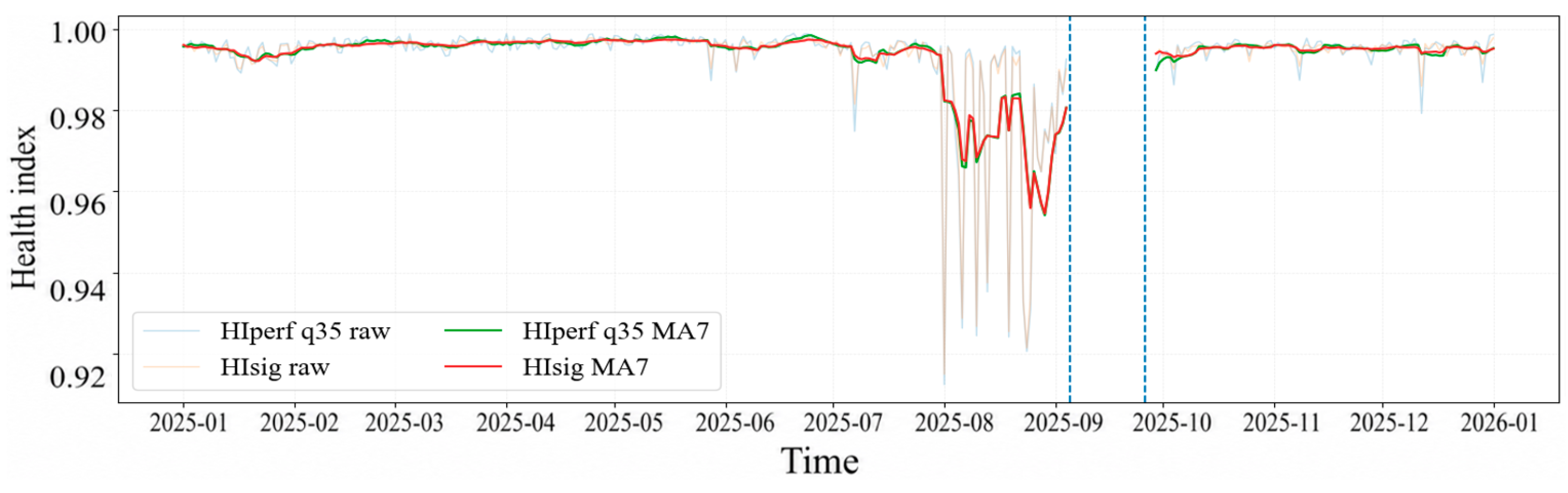
Figure 11 shows the trend comparison between $H{I}_{perf,q35}$ and $H{I}_{sig}$. The two dashed vertical lines indicate the maintenance period from approximately 5 September to 26 September 2025. Before maintenance, both indexes show an obvious decrease and fluctuation around August. During the maintenance period, the data are interrupted. After maintenance, $H{I}_{perf,q35}$ and $H{I}_{sig}$ return to a higher level and remain relatively stable. This result shows that the signal-based health index can follow the main degradation and recovery trend of the performance-side health index.

The feature importance of the XGBoost-based signal-mapping model is shown in Figure 12. The effective features are mainly from shaft-swing channels, while the vibration channel V2 also shows an obvious contribution. The most important features are related to the daily median and mean values of S1, the daily mean value and standard deviation of V2, the high-level daily fluctuation of S6, and the low-level daily fluctuation of S3 and S4. This indicates that shaft-swing signals have a strong response to the performance-side health state, while part of the vibration information also contributes to the construction of $H{I}_{sig}$. In addition, both the daily central level and the distribution range of the monitoring signals are useful for signal-based health representation.

Figure 13 presents the full-sample mapping consistency between $H{I}_{perf,q35}$ and $H{I}_{sig}$. The time-series result shows that $H{I}_{sig}$ follows the main degradation and recovery pattern of $H{I}_{perf,q35}$, while most samples in the scatter plot are distributed close to the 1:1 reference line. For XGBoost, $R^2$, MAE and RMSE were 0.9882, 0.0009, and 0.0012, respectively. These results show that the selected vibration and shaft-swing features contain information strongly consistent with the performance-side health state under full-sample mapping. Independent-test performance is further examined below.

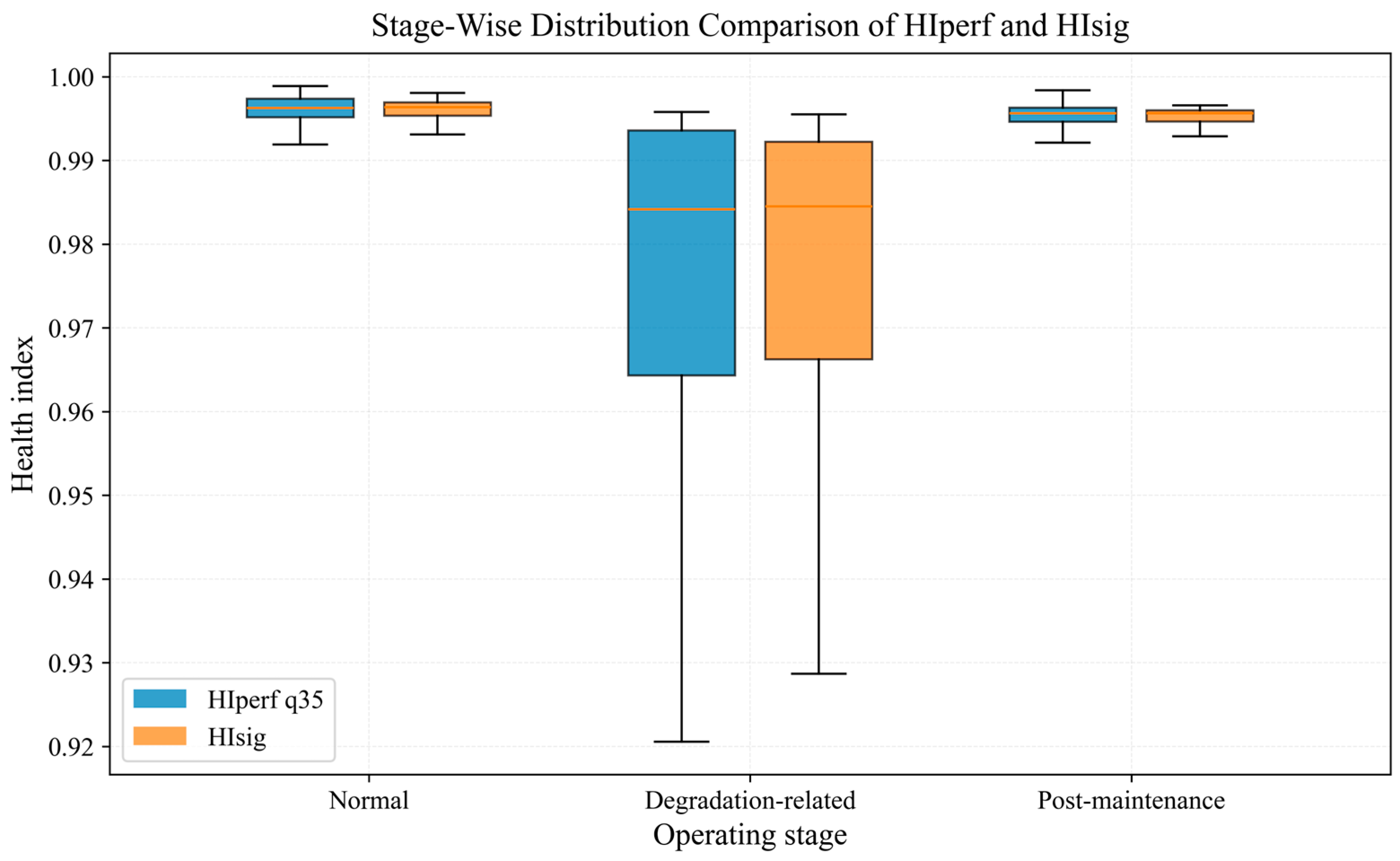
The stage-wise distribution comparison is shown in Figure 14. In the normal stage, the mean values of $H{I}_{perf,q35}$ and $H{I}_{sig}$ are both 0.9958. In the degradation-related stage, the mean values decrease to 0.9721 and 0.9723, respectively. In the post-maintenance stage, the mean values recover to 0.9950 and 0.9951, respectively. The two indexes show similar changes among different stages. This result indicates that the selected vibration and shaft-swing signals can reflect the degradation and recovery process described by the performance-side health index.

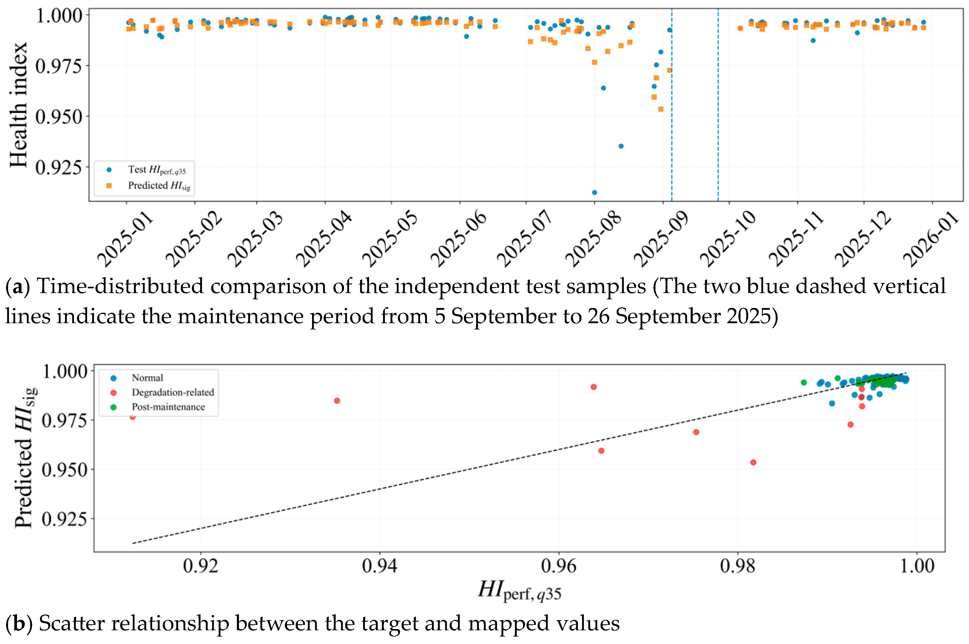
To further evaluate the stability of the mapping relationship on unseen samples, repeated stage-stratified independent testing was conducted for XGBoost, GBDT, and Random Forest. In each of the 20 runs, the daily samples were randomly divided into training and test sets at a ratio of 7:3, using the normal, degradation-related, and post-maintenance stage labels for stratification. XGBoost was retained as the main mapping model based on the full-sample comparison in Table 4. Therefore, Figure 15 presents a representative XGBoost independent-test result. The representative run was selected as the run whose MAE was closest to the median XGBoost MAE across the 20 repeated tests, rather than the run with the lowest test error.

Figure 15 presents a representative independent-test result of the selected XGBoost model. The representative run was selected according to the median MAE over the 20 repeated stage-stratified tests, rather than according to the best test result. Across the 20 runs, XGBoost obtained a mean MAE of 0.0042 and a mean RMSE of 0.0099. For the representative run shown in Figure 15, the MAE and RMSE were 0.0041 and 0.0096, respectively.

As shown in Figure 15a, the mapped $H{I}_{sig}$ values generally follow the variation of the independent-test $H{I}_{perf,q35}$ samples. The prediction errors are relatively small during the normal and post-maintenance stages. As shown in Figure 15b, most normal and post-maintenance samples are distributed close to the 1:1 reference line. Larger deviations mainly occur for a limited number of low-value samples during the degradation-related stage. These results indicate that the selected vibration and shaft-swing features retain a stable mapping relationship with the performance-side health index on unseen daily samples, although the mapping of severe low-value degradation samples remains more difficult.

Overall, the full-sample results demonstrate strong consistency between $H{I}_{sig}$ and $H{I}_{perf,q35}$. The repeated stage-stratified independent tests further show that the selected vibration and shaft-swing features retain a stable mapping relationship with the performance-side health index on unseen daily samples. XGBoost maintains relatively low mapping errors across the repeated tests, while larger deviations mainly occur for a limited number of low-value samples during the degradation-related stage. Therefore, $H{I}_{sig}$ is used as a signal-based representation of the observed degradation trend rather than as a future-state prediction model.

The proposed method was mainly developed and validated for Francis turbine-generator units. For other Francis units, the overall framework can be reused, but the condition boundaries, operating regions, envelope parameters, sensitive signal channels, and mapping models should be retrained using unit-specific data. For other turbine types, the condition-partitioning method may require further adjustment. For example, the runner blade angle should be considered for Kaplan units, while generation and pumping modes should be modeled separately for reversible pump-turbines.

5. Conclusions

In this study, a condition-aware performance health index and multi-source signal-mapping method is proposed for degradation trend identification of hydropower units. The main conclusions are as follows.

First, water head was used as a prior constraint to divide the hydraulic boundary. Then, FCM clustering was used in each head layer to obtain different operating regions. The results show that the proposed partitioning method can reduce the influence of mixed operating conditions. Second, a high-quantile performance envelope was built in each operating region. Based on the optimal power benchmark, the performance health index $H{I}_{perf}$ was constructed, and its daily q35 series was used for degradation trend extraction. The results show that $H{I}_{perf}$ can reflect the deviation between actual power and optimal power. The smoothed daily trend shows an obvious decrease before maintenance and a recovery after maintenance. Third, vibration and shaft-swing signals were used to construct the signal-based health index $H{I}_{sig}$. The mapping result shows that $H{I}_{sig}$ has a similar trend to $H{I}_{perf}$. Shaft-swing features have a stronger contribution than vibration features, which indicates that shaft-swing signals are more sensitive to the performance degradation of the studied unit. Repeated stage-stratified independent testing further showed that the selected vibration and shaft-swing features retained a stable mapping relationship with the performance-side health index on unseen daily samples. For XGBoost, the mean MAE and RMSE over the 20 repeated tests were 0.0042 and 0.0099, respectively, although larger deviations remained for a limited number of low-value degradation samples.

Overall, the proposed method can evaluate the performance degradation of hydropower units under complex operating conditions. It also provides a way to link performance degradation with dynamic monitoring signals. The method can provide a reference for health assessment and degradation trend analysis of hydropower units. This framework is intended for daily-scale and long-term degradation trend assessment under steady-state operating regimes. Transient events, such as rapid load regulation and start-stop processes, are excluded from the health index construction proposed in this study and are not directly evaluated here.

References

1. Shi, L.; Duanmu, C.; Wu, F.; He, S.; Lee, K.Y. Optimal allocation of energy storage capacity for hydro-wind-solar multi-energy renewable energy system with nested multiple time scales. J. Clean. Prod. 2024, 446, 141357. [Google Scholar] [CrossRef] [Scilit]
2. Zhao, Z.; Ding, X.; Behrens, P.; Li, J.; He, M.; Gao, Y.; Liu, G.; Xu, B.; Chen, D. The importance of flexible hydropower in providing electricity stability during China’s coal phase-out. Appl. Energy 2023, 336, 120684. [Google Scholar] [CrossRef] [Scilit]
3. Jin, X.; Liu, B.; Liao, S.; Cheng, C.; Zhang, Y.; Jia, Z. Assessing hydropower capability for accommodating variable renewable energy considering peak shaving of multiple power grids. Energy 2024, 305, 132283. [Google Scholar] [CrossRef] [Scilit]
4. Wang, Y.; Liu, Y.; Li, X.; Wang, T.; Xu, Z.; Guo, P.; Liao, B. Intelligent recognition for operation states of hydroelectric generating units based on data fusion and visualization analysis. Int. J. Intell. Syst. 2025, 1, 8850566. [Google Scholar] [CrossRef] [Scilit]
5. Liu, Y.; Xu, Z.; He, Y.; Guo, P.; Mu, K. Acoustic fault diagnosis method for rotating machinery based on improved spectral subtraction and CNN-TCN model. Measurement 2025, 256, 118482. [Google Scholar] [CrossRef] [Scilit]
6. Bai, J.; Che, C.; Liu, X.; Wang, L.; He, Z.; Xie, F.; Dou, B.; Guo, H.; Ma, R.; Zou, H. Fault diagnosis of pumped storage units-a novel data-model hybrid-driven strategy. Processes 2024, 12, 2127. [Google Scholar] [CrossRef] [Scilit]
7. Vashishtha, G.; Kumar, R. Autocorrelation energy and aquila optimizer for MED filtering of sound signal to detect bearing defect in Francis turbine. Meas. Sci. Technol. 2021, 33, 015006. [Google Scholar] [CrossRef] [Scilit]
8. Zhao, W.; Presas, A.; Egusquiza, M.; Valentín, D.; Egusquiza, E.; Valero, C. Increasing the operating range and energy production in Francis turbines by an early detection of the overload instability. Measurement 2021, 181, 109580. [Google Scholar] [CrossRef] [Scilit]
9. Bharathi, B.M.R.; Mohanty, A.R. Time delay estimation in reverberant and low SNR environment by EMD based maximum likelihood method. Measurement 2019, 137, 655–663. [Google Scholar] [CrossRef] [Scilit]
10. Robert, G.; Besançon, G. Fault detection in hydroelectric generating units with trigonometric filters. In Proceedings of the 21st IFAC World Congress, Berlin, Germany, 11–17 July 2020; pp. 11686–11691. [Google Scholar]
11. Xu, B.; Chen, D.; Zhang, H.; Li, C.; Zhou, J. Shaft mis-alignment induced vibration of a hydraulic turbine generating system considering parametric uncertainties. J. Sound Vib. 2018, 435, 74–90. [Google Scholar] [CrossRef] [Scilit]
12. Melani, A.H.A.; Silva, J.M.; de Souza, G.F.M.; Silva, J.R. Fault diagnosis based on Petri Nets: The case study of a hydropower plant. IFAC-PapersOnLine 2016, 49, 1–6. [Google Scholar] [CrossRef] [Scilit]
13. Chen, F.; Zhao, Z.; Hu, X.; Liu, D.; Kang, Z.; Ma, Z.; Xiao, P.; Yin, X.; Yang, J. Enhancing the safety of hydroelectric power generation systems: An intelligent identification of axis orbits based on a nonlinear dynamics method. Energy 2025, 324, 135864. [Google Scholar] [CrossRef] [Scilit]
14. Lan, C.; Li, S.; Chen, H.; Zhang, W.; Li, H. Research on running state recognition method of hydro-turbine based on FOA-PNN. Measurement 2021, 169, 108498. [Google Scholar] [CrossRef] [Scilit]
15. Dao, F.; Zen, Y.; Qian, J. A novel denoising method of the hydro-turbine runner for fault signal based on WT-EEMD. Measurement 2023, 219, 113306. [Google Scholar] [CrossRef] [Scilit]
16. Li, X.; Xu, Z.; Wang, Y. PSO-MCKD-MFFResnet based fault diagnosis algorithm for hydropower units. Math. Biosci. Eng. 2023, 20, 14117–14135. [Google Scholar] [CrossRef] [Scilit] [PubMed]
17. Dao, F.; Zeng, Y.; Qian, J. Fault diagnosis of hydro-turbine via the incorporation of Bayesian algorithm optimized CNN-LSTM neural network. Energy 2024, 290, 130326. [Google Scholar] [CrossRef] [Scilit]
18. Zhang, L.; Zhou, B.; Wang, S.; Sun, N.; Zheng, H. Wind turbine blade health state assessment based on fuzzy evaluation. J. Phys. Conf. Ser. 2024, 2882, 012041. [Google Scholar] [CrossRef] [Scilit]
19. Sonthalia, A.; Femilda Josephin, J.S.; Varuvel, E.G.; Chinnathambi, A.; Subramanian, T.; Kiani, F. A deep learning multi-feature based fusion model for predicting the state of health of Lithium-Ion batteries. Energy 2025, 317, 134569. [Google Scholar] [CrossRef] [Scilit]
20. Xue, B.; Yu, Y.; Fu, H.; Zhu, J.; Xu, Z. Advanced prognostics techniques for machinery under time-varying operating conditions: A review. Appl. Intell. 2025, 55, 1066. [Google Scholar] [CrossRef] [Scilit]
21. Shan, Y.; Liu, J.; Xu, Y.; Zhou, J. A combined multi-objective optimization model for degradation trend prediction of pumped storage unit. Measurement 2021, 169, 108373. [Google Scholar] [CrossRef] [Scilit]
22. Wang, Y.; Xiao, Z.; Liu, D.; Chen, J.; Liu, D.; Hu, X. Degradation trend prediction of hydropower units based on a comprehensive deterioration index and LSTM. Energies 2022, 15, 6273. [Google Scholar] [CrossRef] [Scilit]
23. Fu, W.; Wang, K.; Zhang, C.; Tan, J. A hybrid approach for measuring the vibrational trend of hydroelectric unit with enhanced multi-scale chaotic series analysis and optimized least squares support vector machine. Trans. Inst. Meas. Control 2019, 41, 4436–4449. [Google Scholar] [CrossRef] [Scilit]
24. Xiong, L.; Liu, J.; Song, B.; Dang, J.; Yang, F.; Lin, H. Deep learning compound trend prediction model for hydraulic turbine time series. Int. J. Low-Carbon Technol. 2021, 16, 725–731. [Google Scholar] [CrossRef] [Scilit]
25. Li, X.; Xu, Z.; Guo, P. Swing trend prediction of main guide bearing in hydroelectric units based on MFS-DCGNN. Sensors 2024, 24, 3551. [Google Scholar] [CrossRef] [Scilit] [PubMed]
26. Ke, Y.; Wang, Q.; Xiao, H.; Luo, Z.; Li, J. Hydropower unit health assessment based on a combination weighting and improved fuzzy comprehensive evaluation method. Front. Energy Res. 2023, 11, 1242968. [Google Scholar] [CrossRef] [Scilit]
27. Wang, W.; Wang, X.; Wang, Z.; Ni, M.; Yang, C. Analysis of internal flow characteristics of a startup pump turbine at the lowest head under no-load conditions. J. Mar. Sci. Eng. 2021, 9, 1360. [Google Scholar] [CrossRef] [Scilit]
28. Sun, L.; Liu, L.; Xu, Z.; Guo, P. Numerical investigation of no-load startup in a high-head Francis turbine: Insights into flow instabilities and energy dissipation. Phys. Fluids 2024, 36, 035142. [Google Scholar] [CrossRef] [Scilit]
Figure 1. Framework of the proposed method.
Energies 19 03780 g001
Figure 2. Simplified waterway layout and sensor arrangement of the studied hydropower unit.
Energies 19 03780 g002
Figure 3. Comparison between raw operating samples and samples within the modeling domain.
Energies 19 03780 g003
Figure 4. Operating condition clusters obtained by prior water-head-guided fuzzy clustering in the G-H-P space.
Energies 19 03780 g004
Figure 5. Fitting relationship between observed P and estimated P o p t .
Energies 19 03780 g005
Figure 6. Sensitivity analysis of smoothed daily H I p e r f trends under different quantile levels.
Energies 19 03780 g006
Figure 7. One-factor sensitivity of the smoothed daily H I p e r f trend to the envelope parameters.
Energies 19 03780 g007
Figure 8. Comparison of the proposed condition-partitioned model with two global quantile GBDT baselines.
Energies 19 03780 g008
Figure 9. Performance envelope modeling and degradation trend based on H I p e r f , q 35 . (The dashed vertical line indicates the beginning of the maintenance period, 5 September 2025).
Energies 19 03780 g009aEnergies 19 03780 g009b
Figure 10. Sensitive-channel ranking for H I s i g mapping.
Energies 19 03780 g010
Figure 11. Trend comparison between H I p e r f , q 35 and H I s i g . (The two blue dashed vertical lines indicate the maintenance period from 5 September to 26 September 2025).
Energies 19 03780 g011
Figure 12. Feature importance of the signal-based mapping model.
Energies 19 03780 g012
Figure 13. Full-sample mapping consistency between H I p e r f , q 35 and H I s i g .
Energies 19 03780 g013
Figure 14. Stage-wise distribution comparison of H I p e r f , q 35 and H I s i g .
Energies 19 03780 g014
Figure 15. Representative independent-test mapping result of the selected XGBoost model: the representative run was selected according to the median MAE over 20 repeated stage-stratified tests.
Energies 19 03780 g015