Power Quality Composite Disturbance Identification Based on CWT–STFT Dual-Modal Fusion and a Lightweight Network

Abstract

With the continuous penetration of renewable energy and power electronic equipment into modern power systems, the occurrence frequency of composite power quality disturbances has increased significantly. The accurate classification of various composite disturbances under strong noise remains a critical technical challenge. The existing single time–frequency transformation methods cannot simultaneously capture transient time-domain details and fine frequency-domain features of steady-state harmonics, while mainstream deep learning classification networks contain redundant parameters and introduce excessive computational overhead, failing to meet the real-time deployment requirements of power edge terminals. To address these limitations, a lightweight Coordinate Attention ResNet network named ResNet–LCA is proposed based on the dual-modal time–frequency fusion of the Continuous Wavelet Transform and Short-Time Fourier Transform. First, the two transforms are implemented separately to generate two groups of complementary time–frequency maps, which are concatenated along the channel dimension to fully extract the coupling features between the steady-state harmonics and the transient impulses. Second, a Haar wavelet subband mean aggregation module is designed for dimensionality reduction with negligible information loss. This module eliminates the channel redundancy introduced by the multimodal fusion and reduces the overall computational overhead at the input stage. Finally, a lightweight residual network integrated with Coordinate Attention is constructed, with Grouped Half-Convolution adopted to compress the model parameters. CA offsets the feature attenuation induced by the lightweight structural design and further improves the model’s noise immunity. A simulation verification was carried out on a simulated dataset covering 25 types of single and superimposed composite disturbances. At a signal-to-noise ratio of 20 dB, the proposed method achieved an average classification accuracy of 97.92%, with only 5.32 M total parameters and a single-sample GPU inference latency of 0.33 ms. Compared with standard ResNet-18 under 20 dB noisy conditions, the total parameter volume was reduced by 52.7%, the inference latency was shortened by 0.13 ms, and the classification accuracy was improved by 0.60 percentage points. The proposed method achieves coordinated optimization of classification accuracy, noise immunity and inference efficiency, and it can provide lightweight technical support for online intelligent power quality monitoring at the edge nodes of microgrids and islanded power systems.

1. Introduction

Driven by dual carbon goals, the construction of new-type power systems has been steadily advanced worldwide. The large-scale integration of renewable energy into the grid, the widespread application of power electronic equipment, the popularization of electric vehicles and other electrified loads, as well as the continuous interconnection of various nonlinear impulse loads, have collectively rendered power quality disturbances characterized by multi-component superposition and time-varying dynamic evolution [1,2]. In weak grid scenarios such as shipboard standalone power systems and renewable energy microgrids, frequent transient events including motor start–stop surges, switching modulation of photovoltaic inverters and intermittent operation of electric arc furnaces readily induce mutual coupling between diverse disturbances such as voltage sags, voltage swells, harmonics, flicker and transient oscillations. Such composite disturbances not only shorten the service lifetime of the precision electrical apparatus and trigger equipment malfunctions but also easily result in the incorrect tripping of relay protection and the islanding lockout of grid-tied converters, thereby seriously threatening the safe and stable operation of AC/DC distribution networks [3]. Therefore, the rapid and high-precision identification of various composite disturbances under strong noisy environments has become a core research requirement for power quality monitoring and governance. Currently, the modeling, detection and performance evaluation of power quality disturbances comply with the international standard IEEE Std 1159-2019 [4], which provides unified criteria for fair performance comparisons among the various identification algorithms.

The conventional power quality disturbance identification approaches can be classified into two categories: traditional machine learning and deep learning algorithms. The traditional methods manually extracted disturbance features using time–frequency analysis tools such as wavelet transform, Variational Mode Decomposition (VMD) and S-transform and then completed the classification based on shallow learning models including support vector machines, probabilistic neural networks and decision trees [5,6,7,8]. Gaouda et al. first verified the feasibility of wavelet transform for power quality disturbance feature extraction, laying the fundamental framework for time–frequency-analysis-based disturbance identification [5]. Nevertheless, limited by fixed-scale parameters, the wavelet transform could only extract single-scale temporal information and could not explore the frequency-domain coupling rules arising from the superposition of multiple disturbances. Janik et al. achieved the automatic classification of multiple disturbances via radial basis function support vector machines and improved the automation level of the disturbance classification [6]. However, the performance of such algorithms relied heavily on manual feature selection, leading to poor generalization across various practical scenarios. Mishra et al. combined the superior time–frequency focusing characteristic of the S-transform with probabilistic neural networks to realize the high-precision classification of various single disturbances, which constituted a representative work under the traditional technical framework [7]. Subsequent studies slightly improved the classification accuracy by optimizing the hyperparameters of the S-transform [9]; however, the inherent shortcomings of manual feature extraction could not be fundamentally resolved. When exposed to intensive noise interference and complex superimposed composite disturbances, the handcrafted features suffered from either redundancy or insufficient information, resulting in weak model adaptability. Furthermore, most traditional algorithms were only validated on ideal noise-free simulated waveforms and thus could not adapt to the complex actual operating conditions of power grids [10].

Freed from the limitations of manual feature engineering, deep learning-based identification methods can be categorized into 1D time-series classification and 2D time–frequency image classification according to signal representation forms. One-dimensional methods directly input the voltage time-series waveforms into convolutional neural networks (CNNs) and long short-term memory (LSTM) networks. Benefiting from simple architectures and convenient deployment, such methods are only applicable to the classification of basic single disturbances [11]. Unfortunately, 1D time-domain representations fail to simultaneously capture transient abrupt variations in the time domain and steady-state harmonic components in the frequency domain. For composite disturbances consisting of harmonics superimposed on transient impulses, such methods show weak feature discriminability and are prone to frequent classification confusion [12], making them incapable of meeting the identification requirements of complex power grids. By contrast, two-dimensional time–frequency mapping algorithms convert one-dimensional time-series signals into two-dimensional images through Continuous Wavelet Transform (CWT), Short-Time Fourier Transform (STFT), Gramian Angular Field (GAF) and other transformation techniques. Convolutional neural networks are adopted to automatically mine deep coupled features, delivering prominent advantages in joint time–frequency characterization; hence, this technical route has evolved into the mainstream research direction in this discipline [13].

A comprehensive review of recent SCI papers in electrical and energy engineering reveals two common limitations existing in the current 2D time–frequency identification frameworks. First, a single time–frequency transformation cannot accomplish complete time–frequency characterization. Restricted by the time–frequency uncertainty principle, CWT enables the adaptive adjustment of time windows and possesses superior frequency resolution for steady-state signals such as harmonics and sustained oscillations. However, the energy of transient impulses is prone to diffuse across the frequency domain, resulting in an unsatisfactory time-domain localization accuracy. STFT adopts a fixed sliding time window to precisely locate the onset and offset moments of transient disturbances, yet it is incapable of finely decomposing each harmonic order. The time–frequency characteristics of the two transformations are inherently complementary [14]. To date, most existing studies constructed the model inputs based on only a single time–frequency transform, which prevented the synchronous extraction of both the steady-state and transient disturbance features [15,16,17]. A small number of dual-modal fusion schemes suffered from feature homogenization problems. For example, both CWT and Synchroextracting Transform (SET) employed wavelet-based kernels, leading to negligible complementary improvements. The time-domain localization error of transient pulses reaches ±3 ms, far worse than the ±0.5 ms localization precision provided by STFT. Although several schemes integrating CWT and VMD components achieved an improved classification accuracy, they still adopted the standard ResNet as the backbone, which introduced a huge parameter volume and an excessive computational cost and could not be deployed on edge terminals [18,19]. Second, a satisfactory trade-off between identification accuracy and computational efficiency is hard to achieve simultaneously. Classical deep networks including ResNet and DenseNet realize a favorable classification accuracy but are plagued by structural redundancy and slow inference speed. Lightweight networks fed with GAF images occupy a small storage space, whereas GAF maps are highly sparse. Under a low signal-to-noise ratio (SNR) of 20 dB, the valid disturbance features are easily submerged by background noise, leading to drastic declines in identification accuracy and insufficient noise immunity robustness [20].

To strengthen the global feature modeling capability, Transformer architectures have been introduced into power quality disturbance classification tasks in recent years. The existing Transformer-based schemes are classified into lightweight hybrid models and high-precision large models, both of which have inherent defects: lightweight CNN–Transformer hybrid networks contain minimal parameters yet deliver poor classification accuracy under heavy noise conditions; multi-scale stacked Transformers attain moderate accuracy improvements at the cost of low inference efficiency caused by multi-branch stacked structures; the vanilla ViT-Base model achieves optimal classification performance with a total parameter volume up to 86 million, whose computational requirements cannot be satisfied by resource-limited power edge terminals [21,22,23,24,25].

In conclusion, the existing approaches cannot achieve a favorable balance among noise immunity, multi-category composite disturbance classification accuracy and inference efficiency. Overall, the current two-dimensional time–frequency representation frameworks possess three prominent deficiencies: (1) most of the paired time–frequency transformations select wavelet algorithms with homologous internal mechanisms (e.g., CWT and SET), triggering severe feature overlap and redundancy, limited complementary effects and inferior transient localization precision; (2) network lightweighting is realized merely via channel pruning or grouped convolution, without auxiliary attention modules to compensate for feature representation loss induced by model compression, making it difficult to balance classification accuracy and computational consumption; (3) the majority of the methods are verified only on simple dual composite disturbances and fixed Gaussian noise environments, lacking systematic simulation validation under practical engineering scenarios involving frequency deviation, non-Gaussian interference and data distribution mismatch.

To tackle the aforementioned research gaps including monotonous time–frequency representation, channel redundancy after dual-modal fusion, poor adaptability to strong noise and excessive computational costs, a lightweight residual network designated ResNet–LCA based on a CWT–STFT dual-modal time–frequency fusion is proposed in this paper. The core contributions of this work are summarized into three aspects:

• A channel-level synergistic fusion mechanism for CWT and STFT is constructed. The orthogonal time–frequency attributes of the two transformations are utilized to implement complementary feature representation, overcoming the drawbacks of incomplete information acquisition from a single transformation and feature redundancy generated by homologous transformation combinations.
• A Haar wavelet subband mean aggregation dimensionality reduction module is elaborately designed. Redundant channels are compressed while valid disturbance features are retained with negligible information loss, cutting down the overall computational overhead of the network from the input stage.
• The residual units are reconstructed with CG-HConv and Coordinate Attention (CA). The lightweight structural design reduces the total parameters and the inference latency; meanwhile, CA compensates for the feature attenuation caused by network slimming and strengthens the noise immunity robustness, eventually realizing a comprehensive optimization of identification accuracy, anti-interference performance and computational efficiency.

Multiple comparative experiments and ablation studies were conducted on a simulated dataset containing 25 types of power quality disturbances to comprehensively verify the effectiveness and the superiority of the proposed method. The remainder of this manuscript is organized as follows. Section 2 elaborates the overall architecture of the proposed method, the time–frequency preprocessing workflow and the detailed design schemes of the lightweight network. Section 3 illustrates the construction process of the simulation dataset and presents simulation results under various noise levels, horizontal comparisons with state-of-the-art algorithms, embedded terminals inference speed tests and modular ablation experiments. Section 4 analyzes the internal mechanism of the CWT–STFT dual-modal time–frequency fusion, describes the trade-off between the identification accuracy and the computational overhead under a lightweight design, determines the root causes of misclassified samples, and defines the applicable boundary of the proposed model. Section 5 concludes the overall research work and prospects potential directions for future extended investigations.

2. Proposed Method

2.1. Overall Pipeline of the Proposed Scheme

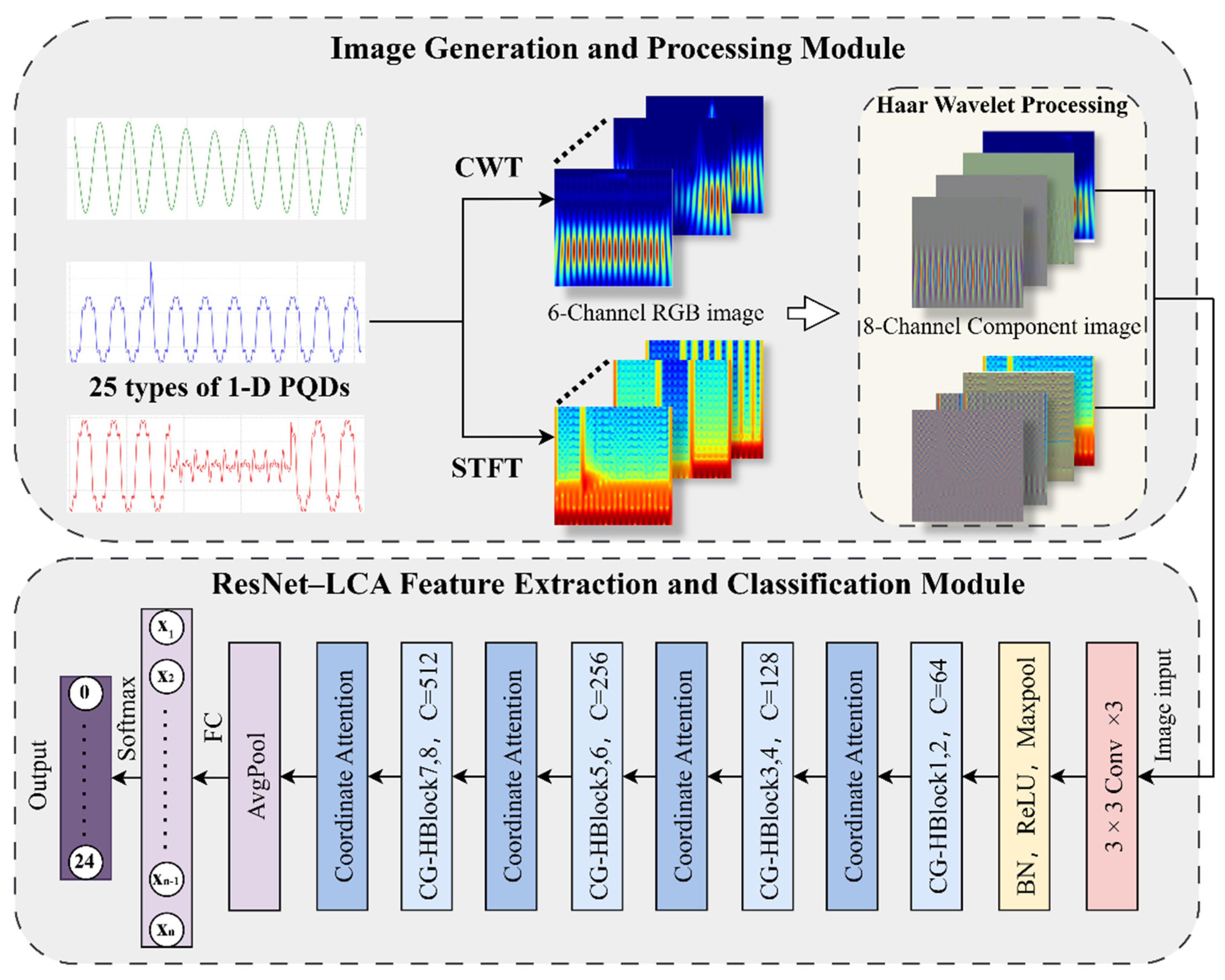
The overall identification framework of the lightweight CWT–STFT dual-modal fusion network proposed in this work is illustrated in Figure 1, and it mainly consists of two stages: time–frequency image generation and preprocessing, as well as feature extraction and classification. In the time–frequency image generation and preprocessing stage, the original disturbance signals are first processed via CWT and STFT to generate two groups of time–frequency maps. Two-dimensional Haar wavelet decomposition and subband mean aggregation are then applied to the two time–frequency maps separately, and the obtained components are concatenated to construct an 8-channel feature map. In the feature extraction and classification stage, the acquired feature map is fed into the lightweight ResNet–LCA network. Deep discriminative features are extracted by CG-HConv and CA mechanisms, and the final identification results are output by the Softmax classifier.

2.2. Multi-Channel Time–Frequency Image Generation and Processing

2.2.1. Time–Frequency Image Generation

Restricted by the time–frequency uncertainty principle, CWT and STFT have inherently complementary characterization properties. Equipped with adaptively adjustable time-scale windows, CWT achieves outstanding performance in extracting precise frequency-domain features of steady narrowband disturbances such as harmonics and sustained oscillations. Nevertheless, the energy of transient impulses tends to spread across the frequency domain, leading to insufficient temporal localization accuracy. In contrast, STFT adopts a fixed sliding window to accurately capture the start and end moments of transient disturbances, yet it cannot resolve densely spaced adjacent harmonic components. To integrate the respective merits of the two transforms, time–frequency maps are generated separately via CWT and STFT in this work.

Let the one-dimensional time-series power quality disturbance signal be defined as $x(n)$, ($n=0,1,\dots ,N-1$). The mathematical expression of STFT is given as

$$S(m,k)={\displaystyle {\displaystyle \sum _{n=0}^{N-1}}x}(n)w(n-m){\mathrm{e}}^{-\mathrm{j}2\pi kn/N}$$

(1)

where m is the time window index, k is the frequency index, and $w(\cdot )$ represents the window function. The calculation formula for CWT is defined as follows:

$$W(a,b)={\displaystyle \frac{1}{\sqrt{\left|a\right|}}}{\displaystyle {\int }_{-\infty }^{\infty }x}(t){\psi }^{*}\left({\displaystyle \frac{t-b}{a}}\right)\mathrm{d}t$$

(2)

where $a$ is the scale parameter, $b$ stands for the translation parameter, and $\psi (t)$ denotes the mother wavelet basis function.

To construct reliable time–frequency representations for power quality disturbance signals, all transformations are implemented on complete original voltage waveforms covering 10 fundamental frequency cycles (0.2 s). The sampling frequency is set to 5120 Hz, and each sample contains 1024 sampling points. The entire waveform is transformed as a whole without any temporal segmentation or truncation, ensuring that the time–frequency maps can fully record the whole evolution process of disturbances from occurrence to recovery.

A Hanning window is utilized for STFT computation, with a window length of 64 sampling points and a frame shift of 16 sampling points, corresponding to an overlapping length of 48 sampling points. The number of FFT calculation points is set to 1024, and zero-padding extension is implemented at signal boundaries. Logarithmic compression is applied to the STFT magnitude matrix to narrow the dynamic range and enhance weak disturbance components.

The Morlet wavelet is selected as the mother wavelet for CWT decomposition. Scales are sampled uniformly and linearly, ranging from 0.1 to 120 with a step size of 1. To realize consistent frequency bandwidth matching between STFT and CWT, only scales corresponding to the 0~2560 Hz frequency band are involved in the calculation. Symmetric reflection padding, the default boundary processing scheme of the PyWavelets library, is adopted for CWT to suppress boundary artifacts.

Min–max normalization is conducted independently on the magnitude matrix of each time–frequency map to scale all numerical values into the interval [0, 1], with no amplitude clipping adopted. Afterwards, the normalized matrices are converted into RGB images through the Jet colormap and uniformly resized to 224 × 224 pixels via bilinear interpolation. Two input tensors are finally obtained: $I_{\mathrm{CWT}}\in {\mathbb{R}}^{224\times 224\times 3}$ and $I_{\mathrm{STFT}}\in {\mathbb{R}}^{224\times 224\times 3}$.

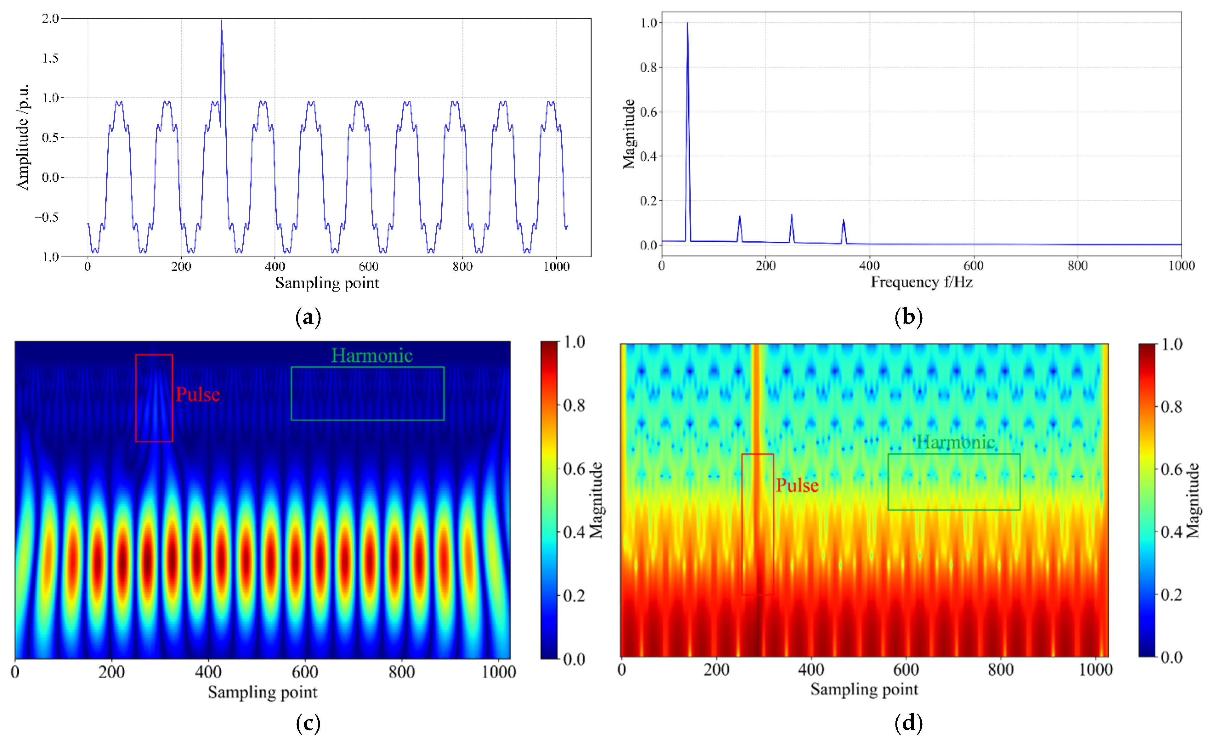
Taking the harmonic-impulse composite disturbance as an example, Figure 2 illustrates its time-domain waveform and frequency spectrum distribution, as well as time–frequency images yielded by the two transforms. As can be observed from the comparison, harmonic stripes are clear and continuous on the CWT time–frequency map, whereas impulse energy diffuses along the frequency axis. On the STFT time–frequency map, the edges of transient impulses remain sharp, while harmonic components appear as blurred bands. The two transforms exhibit obvious complementary properties, which demonstrates that fusing the two types of time–frequency representations enables comprehensive extraction of disturbance features.

2.2.2. Dimensionality Reduction and Fusion of Time–Frequency Images

To reduce the computational overhead of subsequent convolution operations while preserving multi-scale edge features, dimensionality reduction based on two-dimensional Haar wavelet decomposition is performed on both types of time–frequency maps [26]. Taking the CWT time–frequency map $I_{\mathrm{CWT}}\in {\mathbb{R}}^{224\times 224\times 3}$ as an example, two-dimensional Haar wavelet decomposition is carried out independently on each of its three RGB channels. For an image X with a resolution of 224 × 224, the row-wise and column-wise transforms of the 2D Haar wavelet transform are defined in Equations (3) and (4):

$$Y_{i,j/2}={\displaystyle \frac{X_{i,j}+X_{i,j+1}}{\sqrt{2}}},\hspace{1em}{Y}_{i,j/2+112}={\displaystyle \frac{X_{i,j}-X_{i,j+1}}{\sqrt{2}}}$$

(3)

$$W_{i/2,j}={\displaystyle \frac{Y_{i,j}+Y_{i+1,j}}{\sqrt{2}}},\hspace{1em}{W}_{i/2+112,j}={\displaystyle \frac{Y_{i,j}-Y_{i+1,j}}{\sqrt{2}}}$$

(4)

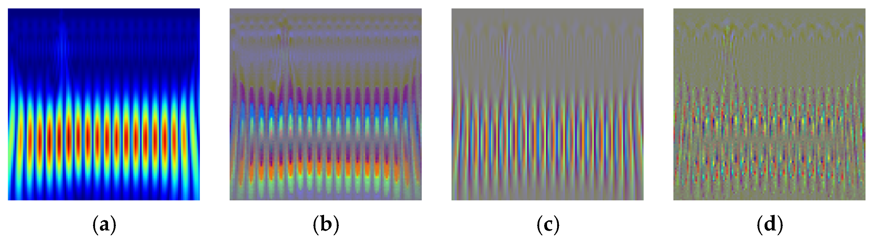
where i = 0, 1, …, 223 and j = 0, 1, …, 222 with a step size of 2. After the above transformation, four subbands including $LL$, $LH$, $HL$, and $HH$ are yielded for each channel, and each subband has a pixel dimension of 112 × 112. The four decomposed subband images of the CWT time–frequency image are illustrated in Figure 3.

Pixel-level averaging is conducted on the corresponding subbands of the three RGB channels. Specifically, the LL subbands from the R, G and B channels are averaged to generate a unified LL component, which is formulated as

$$L{L}_{\mathrm{mean}}={\displaystyle \frac{L{L}_R+L{L}_G+L{L}_B}{3}}\in {\mathbb{R}}^{112\times 112}$$

(5)

Similarly, $L{H}_{\mathrm{mean}}$, $H{L}_{\mathrm{mean}}$ and $H{H}_{\mathrm{mean}}$ are obtained. Thus, $I_{\mathrm{CWT}}$ with the original dimension 3 × 224 × 224 is converted into four component maps of size 112 × 112, denoted as ${\{LL,LH,HL,HH\}}_{\mathrm{CWT}}$.

The identical decomposition and averaging pipeline is applied to the STFT time–frequency map $I_{\mathrm{STFT}}$, producing another set of four subband component maps ${\{LL,LH,HL,HH\}}_{\mathrm{STFT}}$.

Eventually, the four subband components from CWT and the four counterparts from STFT are concatenated along the channel dimension to generate the final 8-channel input feature map:

$$F_{\mathrm{in}}=\mathrm{Concat}\left({\{LL,LH,HL,HH\}}_{\mathrm{CWT}},{\{LL,LH,HL,HH\}}_{\mathrm{STFT}}\right)\in {\mathbb{R}}^{112\times 112\times 8}$$

(6)

This operation downsamples the spatial resolution of feature maps from 224 × 224 to 112 × 112, which reduces the computational overhead of subsequent convolution operations.

2.3. ResNet–LCA Lightweight Classification Network

2.3.1. Overall Network Architecture

• ResNet effectively alleviates the vanishing gradient problem by virtue of cross-layer identity mapping and shortcut connections embedded inside residual blocks. On this basis, targeted improvements are proposed in this paper by combining Grouped Half-Convolution (CG-HConv) and CA, thereby constructing a lightweight network named ResNet–LCA. The structural diagram of the proposed model is shown in Figure 1. The network takes the 8-channel feature map $F_{\mathrm{in}}\in {\mathbb{R}}^{112\times 112\times 8}$ as the input and outputs the probability distribution corresponding to 25 categories of power quality disturbances. Three specific improvements are listed as follows:The original single 7 × 7 convolutional layer is replaced by three stacked 3 × 3 convolutional layers with strides of 2, 1, and 1.
• Residual blocks are reconstructed using CG-HConv to reduce the total parameter quantity of the model.
• Feature extraction is divided into four stages, each containing two residual blocks. Downsampling is conducted between adjacent stages to halve the spatial size and double the number of channels, and a CA module is embedded after each stage.

The detailed architectural parameters of ResNet–LCA are presented in

Table 1. Network architecture of ResNet–LCA.

Stage	Input Tensor Shape	Operation	Output Tensor Shape
Image input	(8,112,112)	8-Channel Component image	(8,112,112)
Initial convolution	(8,112,112)	3 × 3 Conv ×3, s = (2,1,1), p = 1	(64,56,56)
Max pooling	(64,56,56)	3 × 3 MaxPool, s = 2, p = 1,	(64,28,28)
Stage 1-1	(64,28,28)	CG-HBlock1, s = 1, p = 1	(64,28,28)
Stage 1-2	(64,28,28)	CG-HBlock2, s = 1, p = 1	(64,28,28)
Attention 1	(64,28,28)	Coordinate Attention	(64,28,28)
Stage 2-1	(64,28,28)	CG-HBlock3, s = 2, p = 1	(128,14,14)
Stage 2-2	(128,14,14)	CG-HBlock4, s = 1, p = 1	(128,14,14)
Attention 2	(128,14,14)	Coordinate Attention	(128,14,14)
Stage 3-1	(128,14,14)	CG-HBlock5, s = 2, p = 1	(256,7,7)
Stage 3-2	(256,7,7)	CG-HBlock6, s = 1, p = 1	(256,7,7)
Attention 3	(256,7,7)	Coordinate Attention	(256,7,7)
Stage 4-1	(256,7,7)	CG-HBlock7, s = 2, p = 1	(512,4,4)
Stage 4-2	(512,4,4)	CG-HBlock8, s = 1, p = 1	(512,4,4)
Attention 4	(512,4,4)	Coordinate Attention	(512,4,4)
Average pooling	(512,4,4)	Adaptive average pooling	(512,1,1)
Fully connected	(512,1,1)	FC	(25)
Softmax	(25)	Softmax	(25)

.

2.3.2. CG-HConv Residual Blocks

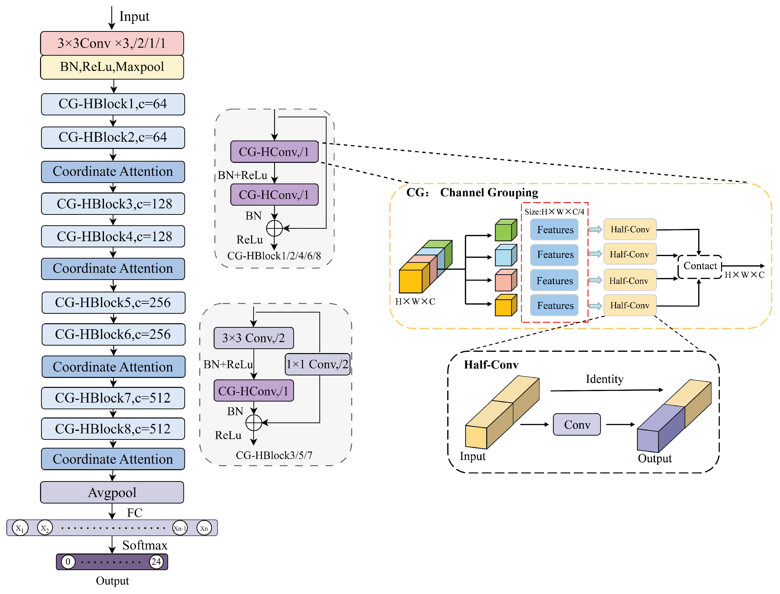
To reduce the total number of model parameters, residual modules are reconstructed based on CG-HConv, and two types of CG-HBlock residual units are designed in this work. The architecture of the proposed CG-HBlock is presented in Figure 4.

The non-downsampling residual block keeps the spatial size of feature maps unchanged. Its main branch consists of two cascaded CG-HConv layers with a stride of 1, while the shortcut branch adopts identity shortcut mapping. The downsampling residual block halves the spatial resolution of feature maps: the main branch first realizes downsampling via a standard 3 × 3 convolution with stride 2, followed by Batch Normalization and ReLU activation, and then passes through one CG-HConv layer with stride = 1. The shortcut branch employs a 1 × 1 convolution with stride 2 to match the channel number and spatial size consistently with the output of the main branch.

Given the input feature tensor $F_{\mathrm{in}}\in {\mathbb{R}}^{C\times H\times W}$, CG-HConv adopts a fixed channel partition strategy with no learnable channel selection weights. All channels are equally divided into four groups in the order of channel indices, and each group contains C/4 channels. Within each channel group, all channels are further split evenly into two parts: the first half of the channels are fed into independent 3 × 3 convolution kernels to extract local spatial features, while the latter half of the channels adopt identity shortcut mapping and skip convolution calculations entirely. After all groups are processed, the output features of each branch are concatenated along the channel dimension. The grouping and channel splitting rules are fixed at network initialization and remain unchanged during the entire training process, without introducing any learnable channel selection parameters.

The overall computation formula of Grouped Half-Convolution is expressed as

$$\left\{\begin{array}{c} F_i=\mathrm{Concat} ({\mathrm{Conv}}_i(F_{\mathrm{in},i}^{(1)}),F_{\mathrm{in},i}^{(2)}), i=1,2,3,4\hfill \\ \mathrm{CG}\text{-}\mathrm{HConv}(F_{\mathrm{in}})=\mathrm{Concat} \left(F_1,F_2,F_3,F_4\right)\in {\mathbb{R}}^{C\times H\times W}\hfill \end{array}\right.$$

(7)

where $F_{\mathrm{in},i}^{(1)}$ and $F_{\mathrm{in},i}^{(2)}$ denote the former and latter sub-channels obtained by halving split of the i-th group of channels derived from the input feature $F_{\mathrm{in}}$.

The forward propagation formulation of the non-downsampling CG-HBlock is defined as

$$F_{\mathrm{out}}=\mathrm{ReLU}\left(\mathrm{BN}\left(\mathrm{CG}\text{-}\mathrm{HConv}\left(\mathrm{ReLU}\left(\mathrm{BN}\left(\mathrm{CG}\text{-}\mathrm{HConv}(F_{\mathrm{in}})\right)\right)\right)\right)+F_{\mathrm{in}}\right)$$

(8)

For the downsampling CG-HBlock, the intermediate feature of the main branch is denoted as

$$F_{\mathrm{mid}}=\mathrm{CG}\text{-}\mathrm{HConv}\left(\mathrm{ReLU}\left(\mathrm{BN}\left({\mathrm{Conv}}_{3\times 3,s=2}(F_{\mathrm{in}})\right)\right)\right)$$

(9)

Then, the final output is

$$F_{\mathrm{out}}=\mathrm{ReLU}\left(\mathrm{BN}(F_{\mathrm{mid}})+{\mathrm{Conv}}_{1\times 1,s=2}(F_{\mathrm{in}})\right)$$

(10)

where ${\mathrm{Conv}}_{3\times 3,s=2}$ refers to the 3 × 3 convolutional layer with stride 2 and ${\mathrm{Conv}}_{1\times 1,s=2}$ denotes the 1 × 1 convolutional layer with stride 2.

2.3.3. Coordinate Attention Mechanism

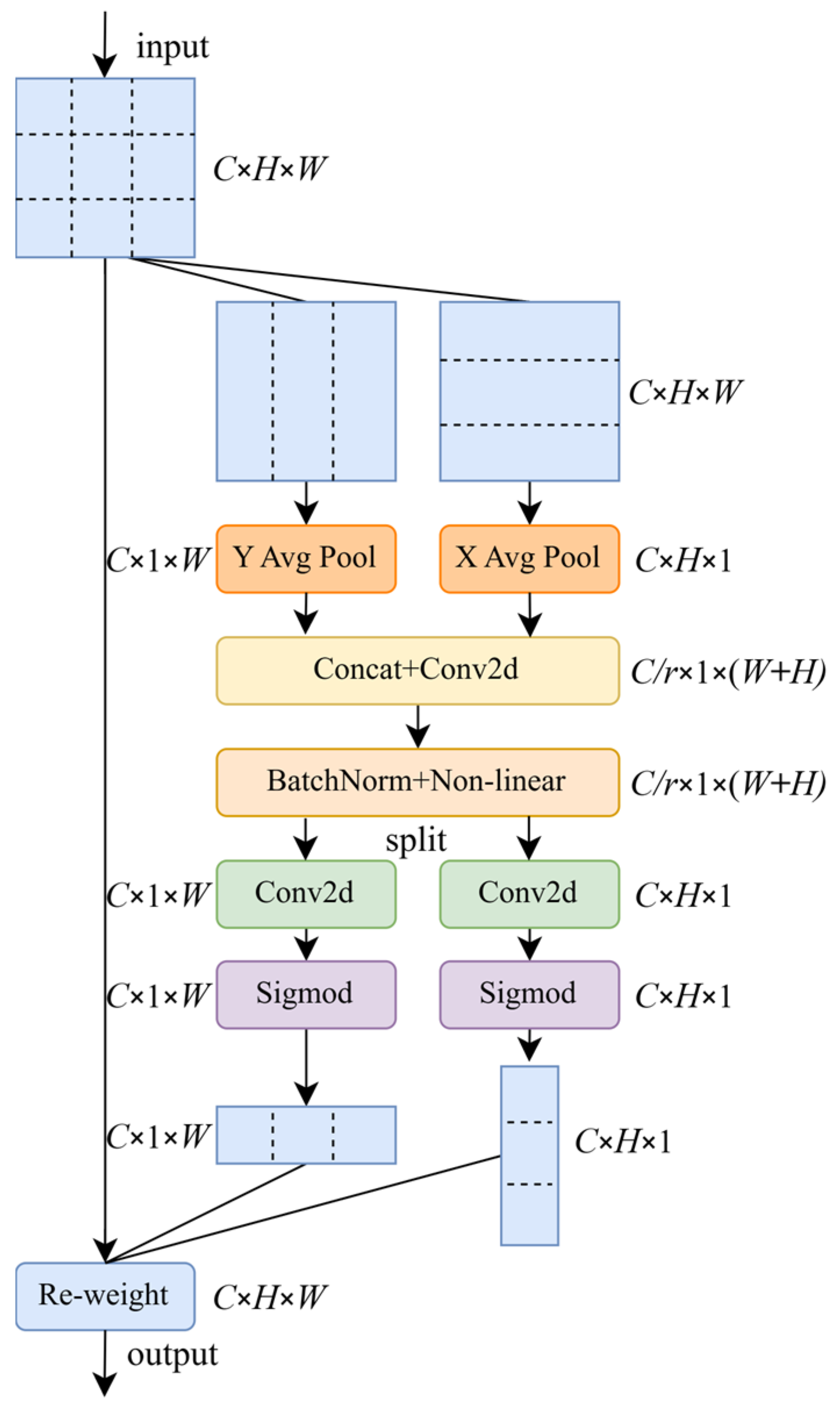
A CA module is embedded after each feature extraction stage [27]. The structure of the Coordinate Attention mechanism is shown in Figure 5. CA conducts global average pooling along the vertical and horizontal directions separately to generate bidirectional attention weights for feature recalibration, while the spatial size and channel count of feature maps remain unchanged.

Given an input feature map $Z\in {\mathbb{R}}^{C\times H\times W}$, global average pooling is implemented along the vertical and horizontal axes:

$$Z_c^{ h}(h)={\displaystyle \frac{1}{W}}{\displaystyle {\displaystyle \sum _{x=0}^{W-1}}{Z}_c}(h,x),\hspace{1em}{Z}_c^{ w}(w)={\displaystyle \frac{1}{H}}{\displaystyle {\displaystyle \sum _{y=0}^{H-1}}{Z}_c}(y,w)$$

(11)

The two directional pooled feature tensors are concatenated along the spatial dimension, then processed sequentially via 1 × 1 convolution, batch normalization and ReLU non-linear activation to obtain the fused compressed feature f. Afterwards, $f$ is evenly split into two independent tensors, $f^h$ and $f^w$, corresponding to the height and width directions, which are utilized to generate the final bidirectional attention weights:

$$g^h=\sigma \left({\mathrm{Conv}}_{1\times 1}(f^h)\right),\hspace{1em}{g}^w=\sigma \left({\mathrm{Conv}}_{1\times 1}(f^w)\right)$$

(12)

Finally, element-wise multiplication is performed between the attention weights and the original input feature map to complete feature recalibration:

$${Z^{\prime }}_c(x,y)=Z_c(x,y)\odot g_c^{ h}(x)\odot g_c^{ w}(y)$$

(13)

The output feature map Z′ of the CA module is fed into the next feature extraction stage.

3. Simulation and Result Analysis

3.1. Simulation Configuration

3.1.1. Power Quality Disturbance Dataset Establishment

To comprehensively evaluate the classification performance and the out-of-distribution generalization capability of the proposed model under complex power quality disturbance scenarios, 25 waveform patterns are constructed in this study in accordance with the typical disturbance categories defined in IEEE Std 1159-2019 [21]. The detailed classification of the 25 power quality disturbance types is listed in

Table 2. Twenty-five categories of power quality disturbances (PQDs) with their corresponding labels.

PQD Category	Label	PQD Category	Label
Normal Signal	C0	Harmonics + Flicker	C13
Voltage Swell	C1	Impulse + Harmonics	C14
Voltage Sag	C2	Harmonics + Oscillation	C15
Harmonics	C3	Flicker + Swell	C16
Flicker	C4	Flicker + Sag	C17
Interruption	C5	Flicker + Oscillation	C18
Impulse	C6	Flicker + Impulse	C19
Oscillation	C7	Swell + Oscillation	C20
Notch	C8	Sag + Oscillation	C21
Spike	C9	Harmonics + Oscillation + Swell	C22
Harmonics + Swell	C10	Harmonics + Oscillation + Sag	C23
Harmonics + Sag	C11	Harmonics + Oscillation + Flicker	C24
Harmonics + Interruption	C12

. These waveforms are generated via the superposition of various disturbances, covering nominal waveforms, 9 types of single disturbances, 12 types of dual composite disturbances, and 3 types of triple composite disturbances. The mathematical formulations and the parametric constraints for all the disturbance modes are detailed in Appendix A.

A total of 18,400 samples are independently generated for each simulation trial. Among them, 1000 samples are allocated for the nominal signal and each single disturbance category; 600 samples are prepared for each dual composite disturbance; 400 samples are assigned to every triple composite disturbance. The fundamental frequency of all the signals is set to 50 Hz, and the sampling frequency is 5120 Hz. Each sample contains 1024 sampling points corresponding to 10 fundamental frequency cycles. All the samples are randomly partitioned into a training set, a validation set and a test set at a ratio of 7:2:1. To mitigate random simulation variations, all the experiments are repeated 20 times independently. A complete dataset is regenerated and repartitioned in each run, and the final evaluation metrics are calculated as the average values across the 20 repeated experiments.

To validate the noise immunity robustness of the proposed model, Gaussian white noise is superimposed on clean waveforms to establish three datasets with fixed SNR levels: 20 dB, 30 dB and 40 dB. In addition, a mixed-SNR dataset is constructed, where the SNR value of each sample is randomly selected with equal probability from the set {20 dB, 30 dB, 40 dB}. Each of the four noise-containing datasets comprises 18,400 samples, leading to a total of 73,600 samples per simulation round.

All the samples are generated through independent random sampling of electrical parameters, rather than batch replication based on fixed parameter templates. For each disturbance category, the key parameters including voltage sag/swell magnitudes, impulse amplitude and duration, oscillation frequency and damping coefficient, flicker modulation index, disturbance duration and initial phase, as well as harmonic and interharmonic amplitudes, are uniformly and randomly sampled within the valid ranges specified by IEEE Std 1159-2019 and the relevant industrial standards for each individual sample. This mechanism ensures a unique parameter combination for every sample. No samples with highly overlapping parameters or nearly identical waveforms exist across the different subsets, and the test set covers parameter configurations that never appear in the training set. Consequently, the model cannot acquire artificially inflated classification accuracy by memorizing fixed waveform templates, and the test set can reliably support an out-of-distribution generalization evaluation.

3.1.2. Training Configuration and Simulation Environment

The proposed ResNet–LCA network is built based on the PyTorch 2.6.0 deep learning framework. The Adam optimizer is adopted for model training. The initial learning rate is set to 0.001, and a cosine annealing learning rate decay strategy is implemented, with the minimum learning rate fixed to 10⁻⁶ and an annealing period of 50 epochs. The training batch size is set to 32, and the maximum number of training epochs is limited to 50. Automatic mixed precision is enabled to accelerate the overall training procedure.

During training, the classification accuracy on the validation set is monitored in real time, and the model weights corresponding to the optimal validation accuracy are preserved. If the validation accuracy shows no improvement for five consecutive epochs, an early stopping mechanism is triggered to terminate training in advance to prevent model overfitting. The detailed hardware and software specifications adopted in the experiments are summarized in

Table 3. System configuration for the simulation.

Hardware	Model	Software	Version
CPU	Intel Core I5-14600KF (USA)	Pytorch	2.6.0
GPU	HP NVIDIA GeForce RTX3080 10 GB (USA)	Python	3.12
RAM	Kingston DDR4 32 GB (USA)	CUDA	12.4
HDD	Western Digital SSD 512 GB (USA)	OS	Windows10 64bit

.

3.2. Comprehensive Performance Evaluation of the Proposed Model

3.2.1. Classification Accuracy Under Multiple SNR Conditions

To thoroughly assess the classification accuracy and noise immunity robustness of the proposed model, four simulation scenarios are designed: three fixed SNR levels (20 dB, 30 dB, 40 dB) and one random mixed-SNR scenario. All the experiments are repeated 20 times independently.

Table 4. Classification accuracy (%) per disturbance category under different SNR conditions.

Label	Category	Mixed	40 dB	30 dB	20 dB
C0	Normal Signal	98.46	99.99	99.15	93.24
C1	Voltage Swell	99.36	98.84	99.85	99.09
C2	Voltage Sag	99.95	99.00	99.35	96.86
C3	Harmonics	99.74	100	100	99.98
C4	Flicker	99.35	100	99.28	99.87
C5	Interruption	99.91	100	99.95	99.96
C6	Impulse	99.97	99.69	99.93	99.02
C7	Oscillation	99.67	100	99.81	99.95
C8	Notch	99.97	99.13	99.82	99.94
C9	Spike	97.15	98.13	97.17	87.41
C10	Harmonics + Swell	99.97	99.85	99.82	99.93
C11	Harmonics + Sag	99.53	99.76	99.85	99.95
C12	Harmonics + Interruption	99.84	98.25	99.86	99.91
C13	Harmonics + Flicker	99.97	99.90	99.87	98.80
C14	Impulse + Harmonics	99.44	99.82	99.88	100
C15	Harmonics + Oscillation	99.97	99.78	99.89	99.90
C16	Flicker + Swell	99.74	99.95	99.79	98.50
C17	Flicker + Sag	99.82	99.91	99.80	96.53
C18	Flicker + Oscillation	99.93	100	99.81	96.96
C19	Flicker + Impulse	99.97	100	99.82	98.20
C20	Swell + Oscillation	99.64	99.86	99.83	98.13
C21	Sag + Oscillation	99.98	100	99.84	97.65
C22	Harmonics + Oscillation + Swell	98.53	98.95	96.65	91.36
C23	Harmonics + Oscillation + Sag	99.85	99.95	99.86	99.83
C24	Harmonics + Oscillation + Flicker	99.96	99.99	99.87	97.09
	Average	99.59	99.63	99.55	97.92

records the per-category classification accuracy for the 25 disturbance types under each condition, while

Table 5. Global classification metrics under diverse noise conditions based on 20 repeated experiments.

SNR Condition	Accuracy (Mean ± SD, %)	95% Confidence Interval/%	Recall /%	F1-Score /%	Kappa
Mixed SNR	99.59 ± 0.18	[99.51, 99.67]	99.42	99.47	0.9930
40 dB	99.63 ± 0.19	[99.55, 99.72]	99.39	99.52	0.9932
30 dB	99.55 ± 0.15	[99.48, 99.62]	99.35	99.44	0.9925
20 dB	97.92 ± 0.32	[97.77, 98.06]	97.64	97.78	0.9753

Note: Recall and F1-score values refer to macro-averaged metrics throughout Table 5.

summarizes the global statistical classification metrics of the model.

The simulation results indicate that the average classification accuracy exceeds 99.5% under the 40 dB, random mixed and 30 dB SNR scenarios. Even under the harsh strong-noise condition of 20 dB, the average accuracy still reaches 97.92%. The maximum standard deviation of accuracy across all the scenarios is merely 0.32%, accompanied by narrow 95% confidence intervals. Meanwhile, the macro-averaged Recall, the macro F1-score and the Cohen’s Kappa coefficient all maintain high values. These results demonstrate that the proposed model achieves outstanding overall classification precision and stable generalization capability within a wide noise range.

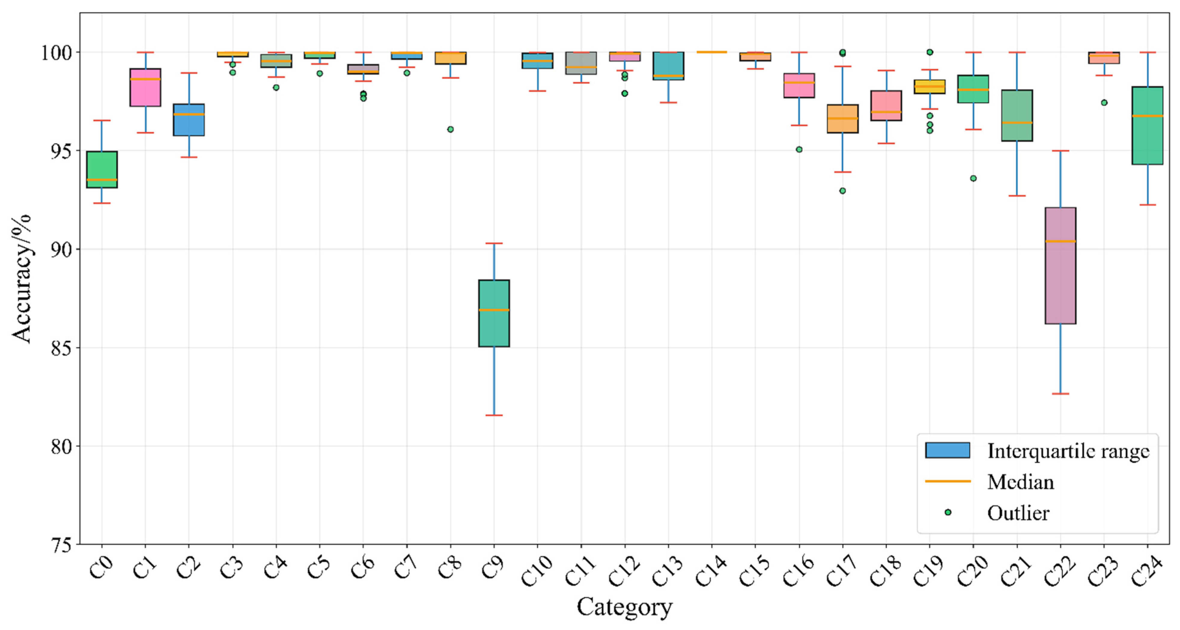
The classification accuracy of nearly all the single disturbances and the dual composite disturbances remains above 96% across all the noise environments. Under high-SNR conditions (40 dB and 30 dB), the classification accuracy of categories C3, C4, C5, C7 and C14 is close to 100%. Nevertheless, two noise-sensitive confusing classes are identified: C9 and C22 are most severely affected by noise interference. At the low SNR of 20 dB, the accuracy of C9 drops to 87.41%, and the accuracy of C22 declines to 91.36%. These two categories constitute the primary bottlenecks restricting the overall classification performance of the model.

To verify the reproducibility of the classification results for all the disturbance types under strong noise, a boxplot of the per-category accuracy at 20 dB SNR is plotted based on the 20 repeated simulation trials, as illustrated in Figure 6. The categories including C3, C4, C5, C7 and C14 exhibit highly stable classification performance, with median values approaching 100% and compact interquartile ranges. In contrast, C0, C9 and C22 yield lower average accuracy with broader box intervals, which signifies more obvious result fluctuations. This observation is completely consistent with the quantitative data listed in Table 4.

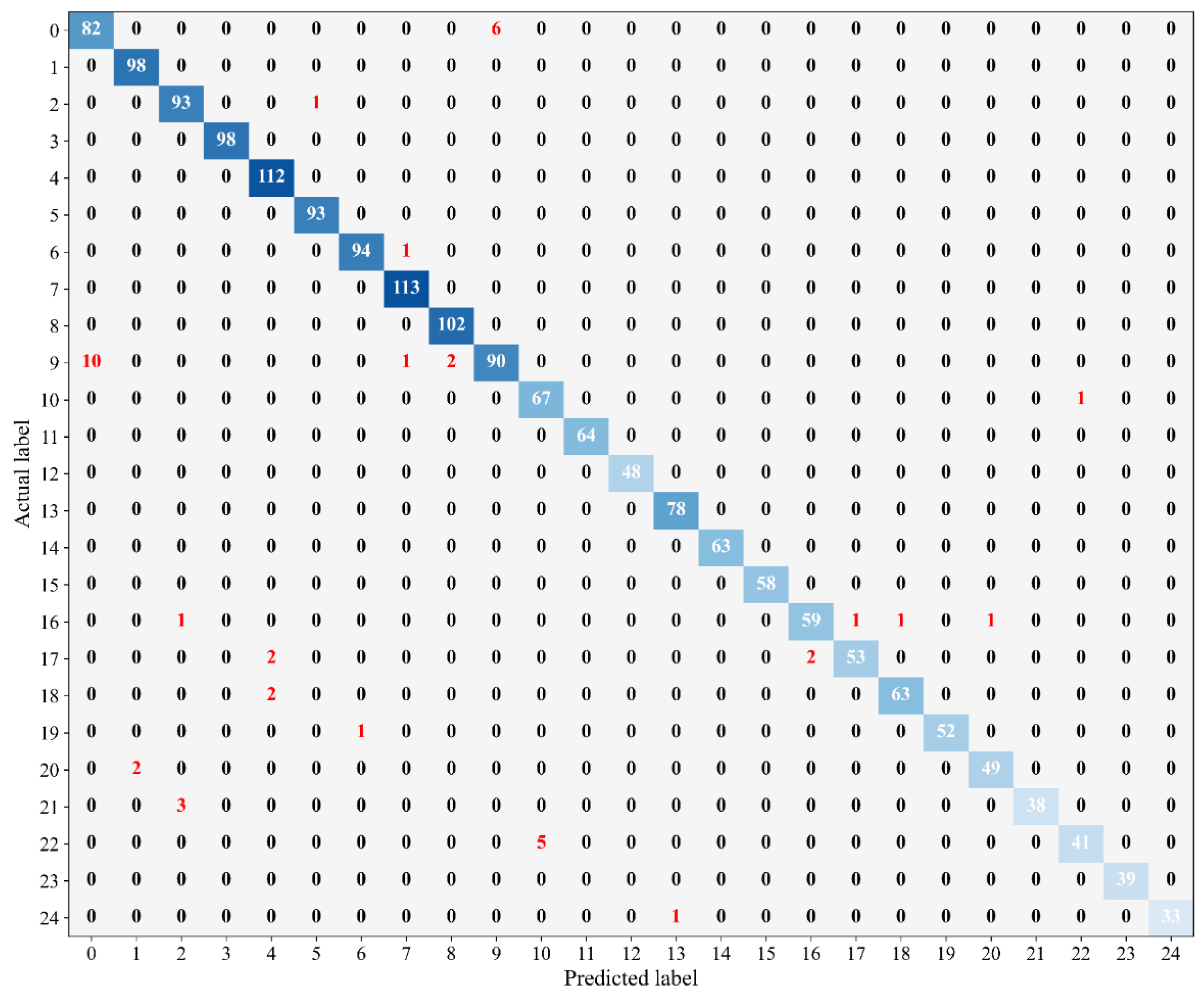
A confusion matrix of the 25 disturbance classes at 20 dB SNR is presented in Figure 7 to elaborate the detailed misclassification patterns under the low-SNR environments. Among the 86 samples of class C0, six are misclassified as C9; out of 103 C9 samples, ten are incorrectly predicted as C0; five samples belonging to C22 are misidentified as C10 within a total of 46 samples.

3.2.2. Comparative Experiments with Classic Convolutional Backbone Networks

Horizontal comparative experiments are carried out under the severest noise condition (20 dB SNR) to quantify the comprehensive performance gaps between the proposed ResNet–LCA and mainstream lightweight networks as well as traditional convolutional neural networks. All the baseline models adopt their original published architectures without any internal modifications. To guarantee fair comparison conditions, all the competing methods share the identical dual-modal time–frequency image input pipeline, training hyperparameters, optimization strategy and hardware operating environment as the proposed scheme.

Four quantitative dimensions are adopted for the performance evaluation: classification accuracy, total parameter count, computational overhead and single-sample GPU inference latency. The comparative results are listed in

Table 6. Performance comparison of different network models at 20 dB SNR.

Model	Accuracy/%	Recall/%	F1-Score/%	Kappa	Params/M	GPU Inference/ms	GFLOPs
ShuffleNet_V2	95.47	94.46	94.83	0.9455	1.47	0.30	0.05
DenseNet-121	97.04	96.24	96.55	0.9657	7.17	0.54	0.77
GoogLeNet-V1	96.82	95.75	96.21	0.9615	6.23	0.40	0.46
EfficientNet_B0	95.83	95.28	95.48	0.9518	3.53	0.34	0.11
MobileNet_V3	96.14	95.53	95.72	0.9552	4.59	0.31	0.07
ResNet-18	97.32	96.67	96.95	0.9678	11.25	0.46	0.53
ResNet–LCA	97.92	97.64	97.78	0.9753	5.32	0.33	0.25

Note: All models were tested on an NVIDIA GeForce RTX 3080, and inference time per sample was averaged over 1000 runs.

. The simulation outcomes demonstrate that ResNet–LCA outperforms all the competing networks in four core classification indicators: overall accuracy, macro Recall, macro F1-score and Cohen’s Kappa coefficient. Taking the standard ResNet-18 as the baseline reference, the proposed network achieves a 0.60 percentage point increase in classification accuracy, with the total parameters reduced by 52.7%, the floating-point operations (GFLOPs) cut by 52.8%, and the single-sample GPU inference time shortened by 0.13 ms.

3.2.3. Comparative Experiments with State-of-the-Art PQD Classification Methods

Table 7. Accuracy comparison with existing state-of-the-art PQD classification methods.

Method	Number of Categories	Contains Triple Disturbances	Contains Mixed SNR	Accuracy/%
				Ideal	Mixed	40 dB	30 dB	20 dB
Reference [20]	25	No	No	98.34	-	98.30	94.24	-
Reference [19]	15	No	No	99.63	-	99.63	99.48	-
Reference [28]	26	Yes	No	97.81	-	-	95.08	92.92
Reference [24]	28	Yes	Yes	99.19	99.81	97.41	92.44	91.94
Reference [16]	21	Yes	No	99.38	-	99.00	98.71	95.00
ResNet–LCA (Ours)	25	Yes	Yes	99.79	99.59	99.63	99.55	97.92

Note: “-” means the original paper did not report accuracy under that noise condition.

presents horizontal comparisons with five mainstream power quality disturbance classification algorithms based on two-dimensional time–frequency images. The competing approaches adopt diverse time–frequency representation strategies (GAF, CWT, MTF) and networks including CNN and Vision Transformer, namely GASF-GADF+ResNet18 [20], CWT-FCCM+ResNet-18 [19], HTC+ResNet-18 [28], GAF+Wave-ViT [24] and MTF+EfficientNet [16].

Considerable discrepancies exist across the published literature in terms of dataset composition, covered disturbance categories and noise test configurations: several studies do not incorporate triple composite disturbances or mixed-SNR test scenarios; in addition, most of the published algorithms have no open-source codes available, making a complete reproduction of their time–frequency transformation pipelines and training hyperparameters infeasible. Accordingly, all the comparative indicators are directly quoted from the original papers to avoid extra errors introduced by manual reconstruction.

As can be observed from Table 7, the proposed ResNet–LCA achieves the highest classification accuracy of 97.92% under the harsh 20 dB strong-noise condition among all the competitors that report this metric. Furthermore, the proposed method attains superior or comparable classification accuracy under 40 dB, 30 dB fixed SNR and random mixed-SNR scenarios.

3.2.4. Engineering Robustness Tests Under Complex Disturbance Conditions

The previous performance validations are implemented under standard Gaussian noise environments. Actual power grids suffer from various adverse operating conditions, including non-Gaussian interference, minor fundamental frequency drift, and distribution mismatch between training and test SNR distributions. Three groups of extended experiments are designed in this Section to evaluate the model performance under non-Gaussian noise, grid fundamental frequency deviation and cross-SNR distribution mismatch scenarios. All the experiments follow unified constraints to ensure fair comparisons. The mathematical models and power limits of all the non-Gaussian noise types are listed in Appendix B.

First, four typical non-Gaussian interference scenarios are constructed: Laplacian noise, impulse noise, background harmonic noise and multi-source mixed noise. All the scenarios are configured at a unified SNR of 20 dB, and the corresponding classification results are summarized in

Table 8. Classification performance under multiple non-Gaussian noise conditions at 20 dB SNR.

Real Noise Types	Accuracy/%	Recall/%	F1-Score/%	Kappa
Gaussian	97.92	97.64	97.78	0.9753
Laplace	98.12	97.68	97.25	0.9748
Impulse	99.06	98.65	98.84	0.9879
Background harmonics	98.72	98.33	98.50	0.9862
Laplace + Impulse + Background harmonics	99.01	98.52	98.75	0.9872

.

The simulation results reveal that the classification accuracy under all the non-Gaussian noise conditions exceeds the Gaussian noise baseline. The accuracy exceeds 99% under the impulse noise and multi-source mixed noise environments, and it remains higher than 98.1% for Laplacian noise and background harmonic noise. The Recall and F1-score values are maintained at high levels across all the test cases.

Subsequently, two frequency deviation test schemes are set up to cover the common frequency fluctuation range in low-voltage distribution networks: continuous random frequency offset, ranging from 49 Hz to 51 Hz with a step size of 0.1 Hz, and fixed steady offsets at 49 Hz, 50 Hz and 51 Hz. The simulation results are presented in

Table 9. Classification performance under grid frequency drift from 49 to 51 Hz.

Real Noise Types	Accuracy/%	Recall/%	F1-Score/%	Kappa
Frequency drift (49–51 Hz)	97.48	97.21	97.34	0.9712
Frequency drift (49 Hz)	97.85	97.58	97.71	0.9742
Frequency drift (51 Hz)	97.79	97.52	97.65	0.9736
Frequency drift (50 Hz)	97.92	97.64	97.78	0.9753

.

Compared with the 50 Hz standard baseline, slight accuracy declines are observed under all the frequency drift conditions. The accuracy reaches 97.85% at the fixed offset of 49 Hz, 97.79% at 51 Hz, and drops to 97.48% under a continuous random offset within 49–51 Hz. Nevertheless, the Recall, F1-score and Kappa coefficients do not undergo obvious degradation.

Finally, cross-SNR generalization experiments are conducted. Three training schemes (20 dB single SNR, 30 dB single SNR, mixed SNR) are combined with various test SNR levels to form six groups of training–test distribution mismatch scenarios, with the results listed in

Table 10. Cross-SNR generalization performance under mismatched training and test SNR conditions.

Training SNR	Test SNR	Accuracy/%	Recall/%	F1-Score/%	Kappa
30 db	Mixed	99.70	99.72	99.71	0.9968
30 db	20 db	97.43	96.96	97.16	0.9707
Mixed	30 db	99.61	99.62	99.60	0.9957
Mixed	20 db	98.57	98.42	98.46	0.9842
20 db	30 db	97.37	96.38	96.77	0.9678
20 db	Mixed	97.34	96.71	96.91	0.9690

.

It can be concluded from Table 10 that the model trained on the 30 dB datasets achieves an accuracy of 99.70% on the mixed-SNR test set. The model trained with the mixed-SNR data obtains accuracies of 99.61% and 98.57% on the 30 dB and 20 dB test sets, respectively. When trained solely on the 20 dB samples, the classification accuracy remains above 97.3% for both the 30 dB and mixed-SNR test scenarios.

3.2.5. Inference Latency and Resource Footprint Tests on Desktop Hardware

Power edge monitoring terminals are universally constrained by limited computing and storage resources. Accordingly, the lightweight degree and the inference efficiency of the model act as core indicators for evaluating its practical engineering deployment potential. In this subsection, single-sample inference latency and hardware resource consumption are measured on multiple desktop CPU and GPU platforms to simulate real-time on-site detection tasks. The batch size is set to one for single-sample inference throughout all the tests, and the quantitative results are provided in

Table 11. Inference latency and memory usage evaluated on different computing platforms.

Hardware	GPU Inference/ms	CPU Inference/ms	VRAM Usage/MB	RAM Usage/MB
CPU (I5-14600KF)	-	2.91	-	31.20
CPU (I7-9750H)	-	9.23	-	31.31
GPU (RTX3080 10 GB)	0.33	-	52.40	-
GPU (RTX4070 super 10 GB)	0.27	-	52.47	-
GPU (GTX1650 4 GB)	2.61	-	52.52	-

.

Two CPU processors are selected for the CPU-side testing: Intel i5-14600KF and Intel i7-9750H, yielding inference latencies of 2.91 ms and 9.23 ms, respectively, with the RAM consumption stabilized between 31.2 MB and 31.3 MB. Three categories of GPUs covering entry-level, mainstream and high-performance graphics cards are tested. The single-sample inference latency on GTX 1650 (4 GB VRAM) reaches 2.61 ms, and the VRAM occupation of all the GPU devices is kept below 53 MB.

3.3. Ablation Studies on Input Pipeline and Network Modules

The previous multi-dimensional comparative experiments verified the comprehensive performance of the complete ResNet–LCA model. In this Section, ablation experiments were conducted to separately quantify the individual contributions of each core component, including the input modal fusion, the front-end time–frequency feature generation schemes, the downsampling operators, and the collaborative combination of the convolution and attention modules.

3.3.1. Ablation Study on Input Modal

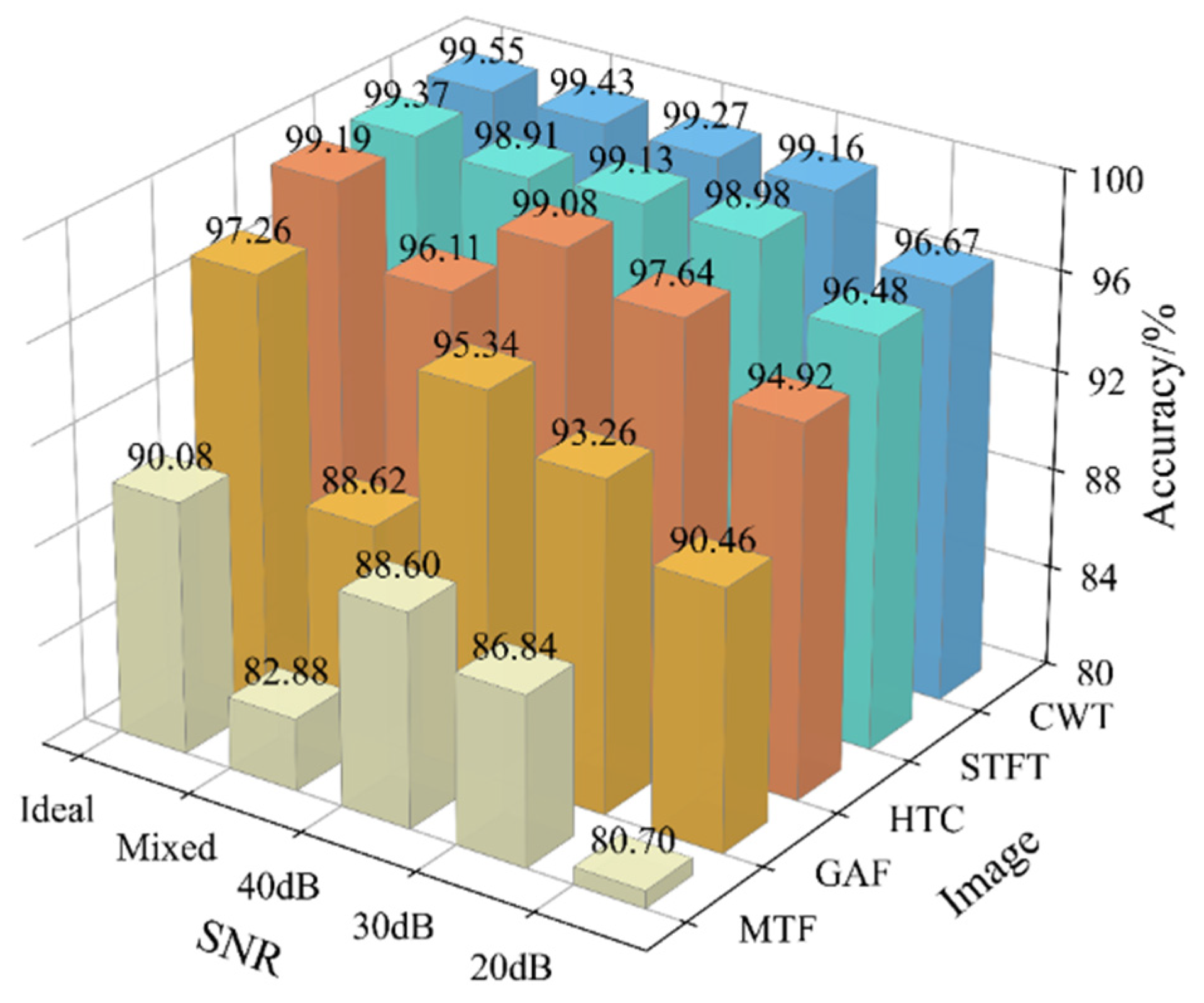
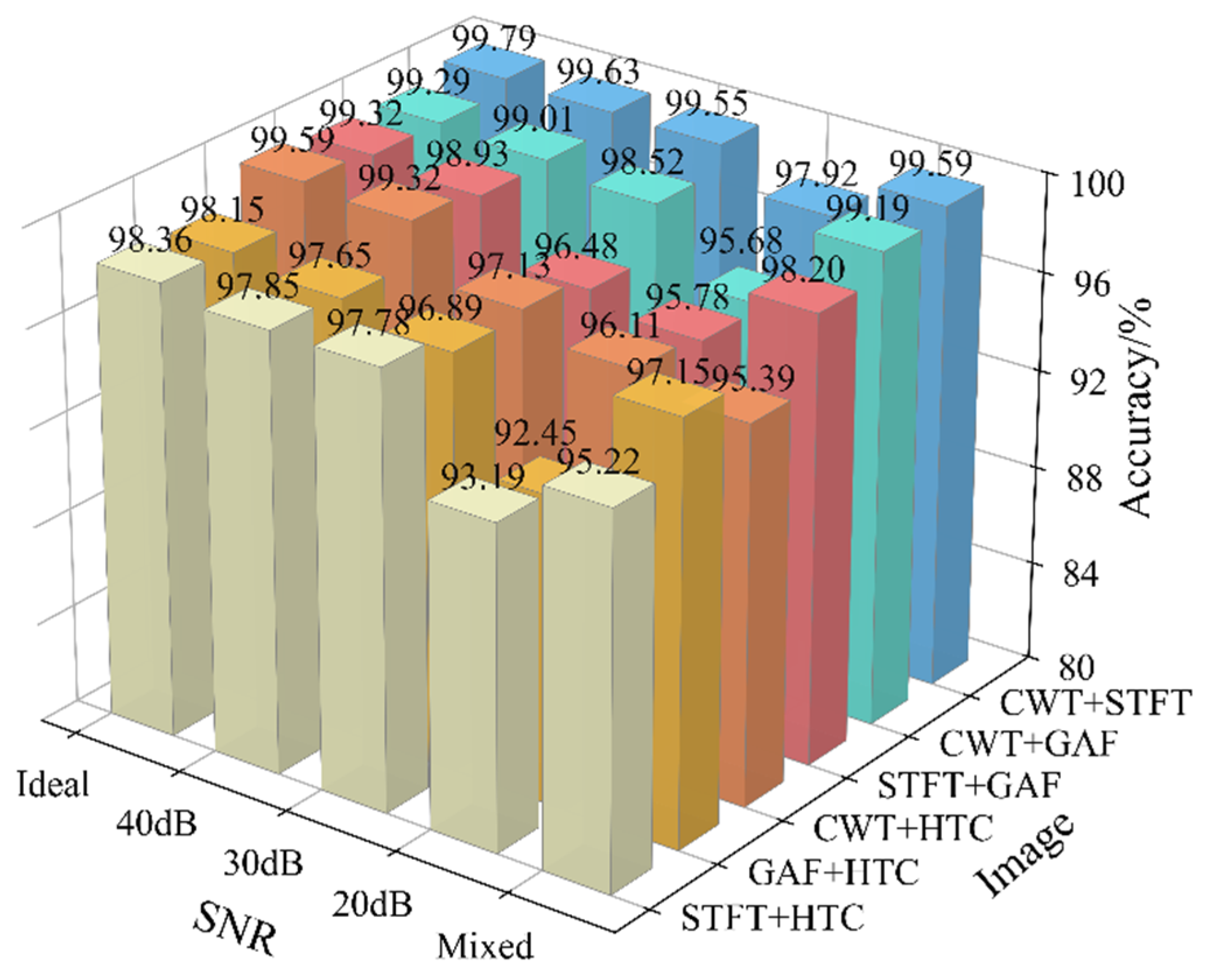
Five distinct time–frequency representations, namely CWT, STFT, GAF, MTF and HTC, were adopted to train the network independently. On the basis of the single-modal simulation results, pairwise combinations of the two best-performing single modalities were constructed to form dual-channel input pipelines. The classification accuracy results are presented in Figure 8 and Figure 9.

It can be observed from the figures that CWT and STFT yielded superior classification performance compared with GAF, MTF and HTC under the single-modal input conditions. The classification accuracy of all the dual-modal fused configurations surpassed that of any standalone single modality, and the CWT+STFT fusion scheme achieved the highest overall accuracy.

The quantitative evaluation metrics across all the SNR scenarios are summarized in

Table 12. Classification accuracy (%) of different input modalities under diverse noise conditions.

Input Modality	Ideal	Mixed	40 dB	30 dB	20 dB
CWT-only	99.55	99.43	99.27	99.16	96.67
STFT-only	99.37	98.91	99.13	98.98	96.48
CWT+STFT Fusion	99.79	99.59	99.63	99.55	97.92
Accuracy Gain vs. Best Single Modality	+0.24	+0.16	+0.36	+0.39	+1.25

Notes: Accuracy Gain = Acc fusion − max (Acc CWT, Acc STFT); mixed SNR means each sample is randomly assigned 20/30/40 dB with equal probability.

. The accuracy gain brought by dual-modal fusion gradually increased as the SNR decreased, peaking at 1.25 percentage points (pp) under the harsh 20 dB strong-noise condition. Specifically, the accuracy was improved by 0.24 pp under noise-free ideal conditions, 0.16 pp under mixed-SNR settings, 0.36 pp at 40 dB, 0.39 pp at 30 dB, and 1.25 pp at 20 dB. At the SNR of 20 dB, the overall classification accuracy of the CWT-only single-modal scheme was 96.67%, which was elevated to 97.92% after adopting the CWT+STFT dual-modal fusion strategy.

Table 13. Classification accuracy (%) of hard and confusing samples under single-modal and fused inputs at 20 dB SNR.

Disturbance Label	CWT-Only Accuracy	STFT-Only Accuracy	Fusion Accuracy	Gain vs. Best Single Modality
C9	84.73	84.44	87.41	+2.68
C22	87.20	84.78	91.36	+4.16

records the category-wise accuracy of two noise-sensitive confusing samples (C9 and C22) under the single-modal and fused input schemes. The accuracy gains were calculated based on the per-class classification results, which intuitively reflect the classification improvement brought by the dual-modal fusion for hard and confusing samples. The simulation data demonstrate that compared with the optimal single modality, the fused input raised the accuracy of class C9 by 2.68 pp and that of class C22 by 4.16 pp. The underlying mechanism accounting for the accuracy variations induced by modal fusion will be elaborated comprehensively in Section 4.

3.3.2. Ablation Study on Front-End Feature Generation Strategies

To validate the effectiveness of the proposed Haar multi-scale mean aggregation front-end preprocessing module, the ResNet–LCA network backbone was fixed, and four groups of comparative experiments were implemented under the SNR condition of 20 dB: (1) two-channel grayscale amplitude input without pseudo-color mapping and Haar wavelet decomposition; (2) direct concatenation of 6-channel RGB images without Haar compression processing; (3) complete 24-channel Haar subband features without RGB channel subband mean aggregation; (4) the proposed 8-channel Haar mean aggregation scheme. The simulation results are listed in

Table 14. Ablation of different front-end feature generation strategies under 20 dB Gaussian white noise.

Simulation Scheme	Params /M	Single Epoch Time/s	GPU Inference/ms	CPU Inference/ms	GFLOPs	Accuracy /%
(1): Gray 2-channel	5.31	73.78	0.92	8.15	0.70	98.23
(2): RGB 6-channel	5.32	85.21	1.17	11.01	0.86	98.37
(3): Haar 24-channel	5.38	43.40	0.37	4.77	0.41	97.94
(4): Ours	5.32	26.35	0.33	2.91	0.25	97.92

Note: 1. Inference time is the average time for one sample (batch size 1) on the test set (1840 samples), averaged over 1000 runs. 2. CG-Hconv: Channel Grouping Half-Convolution. 3. CA: Coordinate Attention mechanism.

.

The grayscale baseline scheme achieved an accuracy of 98.23%, which was comparable to the 6-channel RGB scheme (98.37%). The 24-channel full Haar subband scheme attained an accuracy of 97.94%, marginally higher than the 97.92% achieved by the proposed method. Compared with the grayscale baseline, the proposed Haar multi-scale aggregation scheme led to a slight accuracy reduction of 0.31 pp, with a 0.45 pp accuracy decline relative to the high-precision RGB scheme. Nevertheless, it reduced GPU inference latency to 0.33 ms, CPU inference latency to 2.91 ms, and overall computational overhead to 0.25 GFLOPs. In contrast to the 24-channel Haar scheme, the GFLOPs were reduced by approximately 39%, accompanied by further shortened inference latency.

3.3.3. Ablation Study on Transformation and Downsampling Operators

To verify the synergistic effect of the Haar wavelet downsampling and the subband mean aggregation operators, the CWT–STFT time–frequency input pipeline and the ResNet–LCA backbone were kept unchanged, and comparative tests were conducted under 20 dB noise conditions. The control groups consisted of 24-channel Haar decomposition without mean aggregation, bilinear interpolation downsampling, average pooling downsampling, and strided convolution downsampling. The quantitative outcomes are presented in

Table 15. Ablation of different transformation and downsampling operators under 20 dB Gaussian white noise.

Simulation Scheme	Params /M	Single Epoch Time/s	GPU Inference/ms	CPU Inference/ms	GFLOPs	Accuracy /%
(1): Haar 24-channel	5.38	43.40	0.37	4.77	0.41	97.94
(2): Bilinear 6-channel	5.32	25.38	0.31	2.83	0.23	96.41
(3): Avgpool 6-channel	5.32	25.61	0.31	2.86	0.23	97.55
(4): Strided Conv 6-channel	5.32	25.26	0.30	2.88	0.23	97.76
(5): Ours	5.32	26.35	0.33	2.91	0.25	97.92

.

The proposed method achieved a classification accuracy of 97.92%, exceeding the schemes adopting strided convolution, average pooling and bilinear interpolation downsampling by 0.16 pp, 0.37 pp and 1.51 pp, respectively. All the 6-channel downsampling configurations exhibited a similar computational overhead, and the calculation cost of our proposed scheme remained within the same range. The 24-channel Haar scheme without mean aggregation obtained an accuracy of 97.94%, nearly identical to our approach; however, it required a longer training time and incurred higher inference latency and computational overhead.

3.3.4. Ablation Study on Convolution and Attention Modules

To explore the independent contributions as well as the synergistic benefits of CG-HConv and the CA mechanism, the 8-channel aggregated Haar feature input and the overall network topology were fixed, and only the convolutional units and the attention module configurations were adjusted to design three comparative simulation setups: (1) the standard ResNet residual blocks replaced the CG-HConv blocks in ResNet–LCA, while all the CA modules were retained; (2) the original ResNet–LCA structure was preserved, and all the CA modules were eliminated; (3) the complete ResNet–LCA model integrating CG-HConv blocks and CA was used, which corresponded to the proposed method in this work. The quantitative simulation results are summarized in

Table 16. Ablation of convolution and Coordinate Attention module combinations under 20 dB Gaussian white noise.

Simulation Scheme	Params /M	Single Epoch Time/s	GPU Inference/ms	CPU Inference/ms	GFLOPs	Accuracy /%
(1): Haar 8-channel + standard conv + CA	11.28	54.98	0.40	5.70	0.53	98.09
(2): Haar 8-channel + CG-HConv	5.27	25.59	0.32	2.88	0.25	97.11
(3): Ours	5.32	26.35	0.33	2.91	0.25	97.92

.

Scheme (1) achieved an accuracy of 98.09%, with a parameter volume of 11.28 M and a computational overhead of 0.53 GFLOPs. Scheme (2) adopted lightweight CG-HConv to compress the model: the total parameters were reduced from 11.28 M to 5.27 M, and the floating-point operations were cut from 0.53 GFLOPs to 0.25 GFLOPs (a reduction of 52.8%), while the classification accuracy declined to 97.11%, representing a 0.98 pp drop compared with Scheme (1). Relative to Scheme (2), Scheme (3) increased the parameter count by merely 0.05 M, yet it boosted the classification accuracy from 97.11% to 97.92%, yielding an accuracy improvement of 0.81 pp.

3.4. Quantitative Analysis of Feature Separability

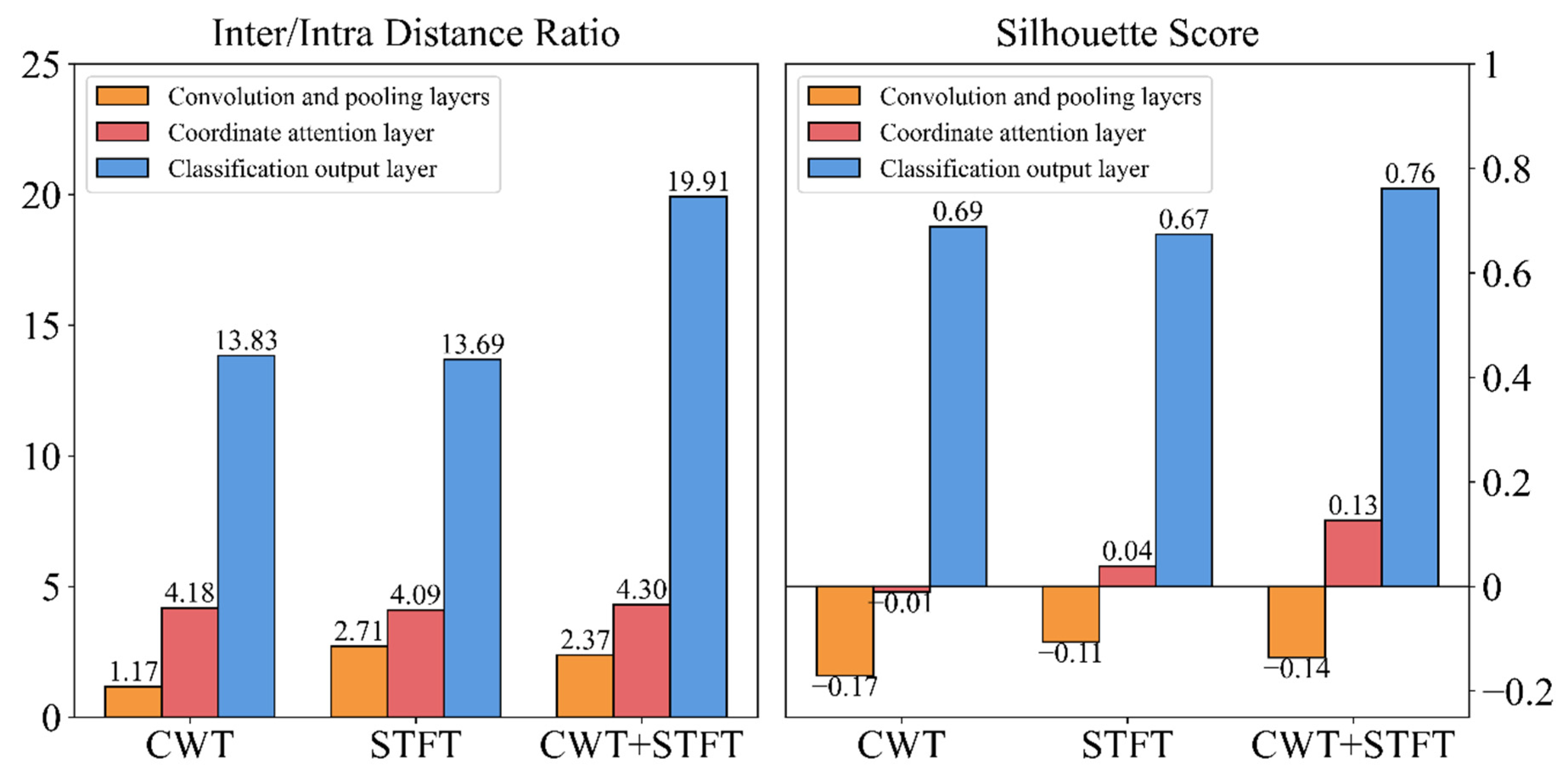
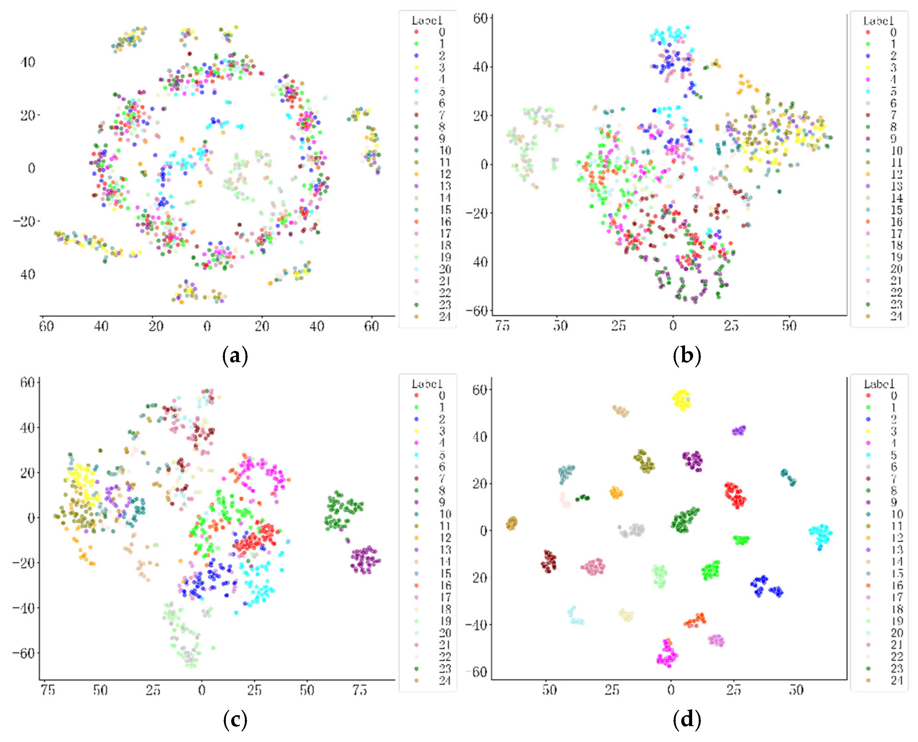
In this Section, three quantitative evaluation metrics, including the inter-class to intra-class distance ratio, the silhouette coefficient, and the feature SNR, are utilized to assess the feature separability of the multi-level network features extracted under different input modalities. The quantitative numerical results are shown in

Table 17. Feature separability metrics at the classification output layer for different input modalities.

Input Modality	Inter/Intra Distance Ratio	Silhouette Score	Feature SNR	Relative Improvement vs. CWT
CWT-only	13.83	0.69	11.41 dB	-
STFT-only	13.69	0.67	11.36 dB	−0.05 dB
CWT+STFT Fusion	19.91	0.76	12.99 dB	+1.58 dB

Notes: Feature signal-to-noise ratio (feature SNR) = 10·log₁₀(D_inter/D intra), where D_inter denotes the average inter-class distance and D intra denotes the average intra-class distance.

; the variations of the feature separability metrics across the different network layers are plotted in Figure 10, and the feature distribution after dimensionality reduction visualization is displayed in Figure 11.

The inter–intra distance ratio values obtained at the CA layer were roughly equivalent among the three input strategies. Nevertheless, from the attention module to the ultimate classification layer, the improvement of feature discriminative ability for the dual-modal fusion scheme was far more prominent than that of the two single-modal counterparts. The variation trend exhibited by the t-SNE dimensionality reduction visualization in Figure 11 is fully consistent with the quantitative indicators recorded in Figure 10 and Table 17.

4. Discussion

4.1. Complementary Mechanism and Gain Sources of CWT–STFT Dual-Channel Fusion

The Heisenberg uncertainty principle constitutes an inherent physical constraint governing time–frequency analysis. A standalone time–frequency transformation cannot simultaneously realize the precise frequency-domain identification of steady-state harmonics and the accurate temporal localization of short-duration transient disturbances. The CWT–STFT dual-channel framework achieves comprehensive information complementarity by leveraging the mutually exclusive design of time–frequency windows between the two transforms.

The CWT employs Morlet wavelets with adjustable scales. It delivers superior frequency resolution in the low-frequency range and can precisely resolve steady-state features including harmonics and sustained oscillations. Nevertheless, its inherent oscillatory tailing effect disperses the energy of millisecond-scale voltage spikes across the frequency domain, resulting in blurred temporal boundaries of transient events. In contrast, the STFT adopts a fixed window length of 64 sampling points (equivalent to 12.5 ms). Though its frequency resolution is limited to Δf = 80 Hz, which prevents the separation of closely spaced harmonic components, it possesses a remarkable temporal positioning capability with an error margin of ±0.5 ms, enabling the sharp delineation of the onset and termination instants of transient disturbances. After the two types of time–frequency spectrograms are concatenated along the channel dimension, the network is capable of jointly learning fine-grained frequency-domain features and dynamic temporal transient variations.

To pinpoint the origin of the performance improvements, the ablation experiments ruled out the possibility that the Jet pseudo-color mapping contributes to the accuracy elevation: the classification accuracy of the two-channel grayscale input scheme is nearly identical to that of the 6-channel RGB image baseline (98.23% versus 98.37%). The feature separability metrics further quantify this enhancement effect; following the dual-modal fusion, the inter-class-to-intra-class distance ratio rises from 13.69 to 19.91, and the feature SNR is boosted by 1.58 dB. Overall, as the environmental SNR declines, the complementary advantages grow more pronounced, yielding a continuous upward trend in classification gains. Under the harsh 20 dB strong-noise condition, the proposed fusion architecture raises the classification accuracy by 1.25 pp compared with the optimal single-modal alternative.

For comparative purposes, reference [18] combines CWT and SET. Since both of the methods construct time–frequency kernels based on the wavelet theory, severe feature overlap and redundancy emerge, leading to a temporal localization error of approximately ±0.3 ms for transient pulses. This study selects CWT and STFT derived from entirely independent mathematical principles. Substantial improvements are observed in both the pulse positioning accuracy (±0.5 ms) and the feature complementary gains, which fundamentally eliminate the issue of redundant feature semantics.

4.2. Accuracy–Efficiency Trade-Off of Lightweight Architecture

To address the channel redundancy induced by the dual-modal feature concatenation, this study proposes a Haar wavelet subband mean aggregation front-end module paired with the lightweight ResNet–LCA backbone network. This design reduces the computational overhead while retaining the discriminative feature information.

Haar wavelet decomposition fully preserves disturbance contours and edge details. The ablation results revealed that retaining all 24 Haar subbands yields only a marginal accuracy gain of 0.02 pp yet significantly prolongs the training epochs and elevates the GFLOPs, which leads to its limited engineering applicability. The adopted RGB subband mean aggregation strategy incurs merely a 0.31 pp accuracy loss compared with the grayscale baseline, compresses the input features into 8 channels, and effectively cuts the front-end computational overhead.

Within the backbone network, CG-HConv evenly partitions all the input channels into four groups. For each group, the first half of the channels undergo convolution calculations, while the remaining channels are directly output via identity shortcut mapping. Benefiting from this structural design, the total parameter volume is reduced by 52.7% relative to ResNet-18. Inevitably, lightweight convolution leads to degraded feature representation capacity. To compensate for such accuracy loss, the CA mechanism is integrated. This module merely adds 0.05 M parameters and introduces an extra inference latency of 0.01 ms, yet it lifts the classification accuracy by 0.81 pp under 20 dB noise, with an overall accuracy compensation rate of roughly 82.7%. The accuracy compensation rate serves as a quantitative indicator for measuring the compensation effect of CA on accuracy losses caused by lightweight convolution. Its numerator refers to the accuracy gain from the attention mechanism (97.92–97.11%), and its denominator corresponds to the overall accuracy decline resulting from the lightweight convolution design (98.09–97.11%).

Meanwhile, standard convolution is retained for all the downsampling stages based on two core considerations. First, this practice avoids the tensor dimension mismatch errors that frequently arise when grouped convolution adopts a stride of two. Second, the feature information is not compressed at nodes with continuously expanding receptive fields, which fully preserves the global spatiotemporal correlation features of the disturbances. The extra parameter volume brought by the standard convolution across the three downsampling layers accounts for approximately 12.7%, calculated via static structural statistics of the network.

4.3. Robustness and Anti-Interference Under Complex Grid Conditions

Noise categories and fundamental frequencies of actual distribution networks fluctuate dynamically. A suite of extended experiments were conducted to explore the model’s robustness boundary, covering non-Gaussian interference, frequency deviation and cross-SNR generalization scenarios.

Different noise types contaminate time–frequency features in distinct patterns and thus deliver divergent classification performances. The classification accuracy under additive white Gaussian noise stands at 97.92%; by comparison, the accuracy climbs to 98.12% under Laplacian noise. Impulse noise forms isolated narrowband spectral peaks on STFT spectrograms that differ sharply from continuous disturbances, which yields the highest accuracy of 99.06%. Background harmonic noise triggers frequency aliasing between background harmonics and fault characteristic harmonics, resulting in a classification accuracy of 98.72%.

When the fundamental frequency deviates within the 49 Hz–51 Hz range, the relative frequency intervals and the topological structures of all the disturbance components remain unchanged. Supported by the adaptive feature weight recalibration capability of CA, the overall accuracy only drops by roughly 0.4 pp. The cross-SNR generalization experiments further verify that the mixed-SNR training scheme enables the model to learn the noise-invariant intrinsic features. Even under harsh training–test distribution mismatch conditions, the classification accuracy stays steadily above 97%, outperforming the models trained with a single fixed SNR value.

Driven by the multi-scale anti-interference capacity of dual-modal fused features and the feature calibration effect of CA, the model maintains a classification accuracy consistently above 97% across all the extended test scenarios, which demonstrates its outstanding adaptive performance for complex power grid environments.

4.4. Misclassification of Hard and Confusing Samples and Model Limitations

Combining confusion matrix statistics and per-class accuracy analysis of hard samples, two primary types of difficult inputs exist, reflecting the inherent performance limitations of two-dimensional static time–frequency representations.

Class C9 corresponds to low-magnitude transient disturbances. Its amplitude ranges from 1.1 to 1.4 times the rated voltage with an extremely short duration of 0.2–1 ms. Under 20 dB noise, its transient energy is easily submerged by background noise, and the corresponding time–frequency maps share a high similarity with the nominal signal C0, leading to the lowest classification accuracy of 87.41% across the full dataset.

The second type consists of triple superimposed coupled composite disturbances. The classification performance varies with the internal coupling modes. Class C23 features distinct voltage sag temporal boundaries and reaches an accuracy of 99.83%; the periodic textures of C24 are prone to blurring under noise and deliver moderate accuracy; the baseline elevation aggravates the frequency aliasing for C22. In addition, the fixed 80 Hz frequency resolution of STFT, jointly determined by a 64-point window and a 5120 Hz sampling frequency, cannot resolve the overlapping harmonic and oscillation components. As a result, its accuracy falls to 91.36%, and most of the samples are misclassified as C10 (harmonics superimposed on voltage swell). This phenomenon confirms that the two-dimensional static images cannot thoroughly eliminate frequency aliasing triggered by mild amplitude distortion.

Three inherent constraints exist for the proposed method: first, data limitation, in which all the samples are generated via numerical simulation complying with IEEE Std 1159-2019 without incorporating unmodeled on-site factors such as three-phase imbalance and sensor drift; second, transformation limitation, whereby the fixed window length of the STFT retains a constant frequency resolution of 80 Hz, which inherently restricts the classification accuracy for disturbances with closely spaced harmonic components; third, deployment limitation, wherein current inference latency metrics are only measured on desktop CPUs and mainstream consumer-grade GPUs, and verification experiments on resource-constrained embedded terminals including Jetson series chips and ARM Cortex-A/NPU platforms have not yet been completed.

5. Conclusions

To tackle the prominent challenges of new-type power systems, including weak noise immunity, excessive parameter overhead and poor adaptability to edge terminals in composite power quality disturbance identification, this paper proposes a lightweight residual network named ResNet–LCA based on a CWT–STFT dual-modal time–frequency fusion. The coordinated optimization of classification accuracy, anti-interference capacity and inference efficiency is realized through the synergistic design of a complementary time–frequency characterization, a front-end dimensionality reduction and an attention-assisted lightweight architecture.

The simulation results revealed that under the 20 dB strong-noise scenario, the proposed method achieves an average classification accuracy of 97.92%. The total parameter volume of the model only reaches 5.32 M, and the single-sample GPU inference latency is 0.33 ms. This algorithm can serve as a feasible technical solution for edge intelligent monitoring under weak grid operation conditions.

The dual-channel fused feature representation system built by exploiting the inherent complementary properties of CWT and STFT breaks two major technical bottlenecks: the incomplete feature information captured by single time–frequency transforms and the feature redundancy of previous homogeneous fusion schemes. Compared with the optimal single-modal scheme, the dual-modal fusion architecture lifts the classification accuracy by 1.25 pp and increases the inter-class-to-intra-class distance ratio by 44.0%. As the SNR gradually declines, the classification gains from dual-modal fusion show an overall upward trend and peak at 20 dB, which fully verifies that the performance improvements stem from the intrinsic physical coupling of the dual-modal time–frequency features rather than from artificial pseudo-features.

CG-HConv replaces the standard residual units to eliminate the channel and computational overhead introduced by dual-modal concatenation, reducing the model’s parameter volume by 52.7% compared with ResNet-18. Meanwhile, the Haar wavelet subband mean aggregation front-end is adopted for dimensionality reduction. Relative to the high-precision RGB baseline, it only incurs a 0.45 pp accuracy loss while shortening the GPU inference latency from 1.17 ms to 0.33 ms. Combined with CA to compensate for the feature degradation brought by the lightweight design, the computational overhead is drastically reduced with a negligible sacrifice of classification performance, which well balances the feature representation capacity and the dual storage/computing constraints of edge deployment.

The generalization tests across multiple operating conditions verified that the model maintains a classification accuracy above 97% under harsh scenarios including non-Gaussian noise, 49–51 Hz fundamental frequency drift and training–test distribution mismatch. On general CPUs, the single-sample inference latency is merely 2.91 ms. With low resource consumption and broad hardware compatibility, the proposed model possesses strong environmental robustness and promising practical deployment potential for power edge monitoring terminals.

To mitigate the constraints stemming from a fixed frequency resolution, adaptive time–frequency transformation algorithms can be explored in subsequent studies. Non-overlapping parameter experiments and field power grid data will enable the rigorous evaluation of the model’s out-of-distribution generalization performance. Furthermore, investigations into quantization acceleration and embedded terminals will serve to build a basis for future practical engineering deployment.

References

1. Wang, F.; Quan, X.Q.; Ren, L.T. Review of Power Quality Disturbance Detection and Identification Methods. Proc. CSEE 2021, 41, 4104–4121. [Google Scholar] [CrossRef]
2. Letha, S.S.; Bollen, M.H.J.; Busatto, T.; Espin Delgado, A.; Mulenga, E.; Bakhtiari, H.; Sutaria, J.; Ahmed, K.M.U.; Nakhodchi, N.; Sakar, S.; et al. Power Quality Issues of Electro-Mobility on Distribution Network—An Overview. Energies 2023, 16, 4850. [Google Scholar] [CrossRef]
3. Altun, B.; Alpsalaz, F.; Uzel, H.; Türkay, Y. Explainable Deep Learning Based Classification for Power Quality Disturbances in Renewable-Energy-Integrated Distribution Networks. IET Renew. Power Gener. 2026, 20, e70269. [Google Scholar] [CrossRef]
4. IEEE Standard 1159-2019; IEEE Recommended Practice for Monitoring Electric Power Quality. IEEE: New York, NY, USA, 2019.
5. Gaouda, A.M.; Kanoun, S.H.; Salama, M.M.A.; Chikhani, A. Wavelet-Based Signal Processing for Disturbance Classification and Measurement. IEE Proc.-Gener. Transm. Distrib. 2002, 149, 310–318. [Google Scholar] [CrossRef]
6. Janik, P.; Lobos, T. Automated Classification of Power-Quality Disturbances Using SVM and RBF Networks. IEEE Trans. Power Deliv. 2006, 21, 1663–1669. [Google Scholar] [CrossRef]
7. Mishra, S.; Bhende, C.N.; Panigrahi, B.K. Detection and Classification of Power Quality Disturbances Using S-Transform and Probabilistic Neural Network. IEEE Trans. Power Deliv. 2008, 23, 280–287. [Google Scholar] [CrossRef]
8. Achlerkar, P.D.; Samantaray, S.R.; Manikandan, M.S. Variational Mode Decomposition and Decision Tree Based Detection and Classification of Power Quality Disturbances in Grid-Connected Distributed Generation System. IEEE Trans. Smart Grid 2018, 9, 3122–3132. [Google Scholar] [CrossRef]
9. Tang, Q.; Qiu, W.; Zhou, Y. Classification of Complex Power Quality Disturbances Using Optimized S-Transform and Kernel SVM. IEEE Trans. Ind. Electron. 2020, 67, 9715–9723. [Google Scholar] [CrossRef]
10. Zhang, W.; Zhang, X.; Zhang, W.; Wang, Y. Multilabel Classification of Complex Power Quality Disturbances via Label-Semantics Fusion and Transformer Encoder. IEEE Trans. Instrum. Meas. 2026, 75, 9002312. [Google Scholar] [CrossRef]
11. Cen, S.; Kim, D.O.; Lim, C.G. A Fused CNN-LSTM Model Using FFT with Application to Real-Time Power Quality Disturbances Recognition. Energy Sci. Eng. 2023, 11, 2267–2280. [Google Scholar] [CrossRef]
12. Xi, Y.; Li, X.; Zhou, F.; Tang, X.; Li, Z.; Zeng, X. Classification of Multiple Power Quality Disturbances Based on Continuous Wavelet Transform and Lightweight Convolutional Neural Network. Energy Sci. Eng. 2023, 11, 3232–3249. [Google Scholar] [CrossRef]
13. Qiu, W.; Tang, Q.; Liu, J.; Yao, W. An Automatic Identification Framework for Complex Power Quality Disturbances Based on Multifusion Convolutional Neural Network. IEEE Trans. Ind. Inform. 2020, 16, 3233–3241. [Google Scholar] [CrossRef]
14. Priyadarshini, M.S.; Bajaj, M.; Prokop, L.; Berhanu, M. Perception of Power Quality Disturbances Using Fourier, Short-Time Fourier, Continuous and Discrete Wavelet Transforms. Sci. Rep. 2024, 14, 3443. [Google Scholar] [CrossRef] [PubMed]
15. Pérez-Anaya, E.; Jaén-Cuellar, A.Y.; Elvira-Ortiz, D.A.; Romero-Troncoso, R.d.J.; Saucedo-Dorantes, J.J. Methodology for the Detection and Classification of Power Quality Disturbances Using CWT and CNN. Energies 2024, 17, 852. [Google Scholar] [CrossRef]
16. Liu, Y.H.; Shi, W.F.; Jiang, J.Q.; Fu, C.H.; Xie, J.L. Identification of Shipboard Power Quality Disturbances Based on MTF-EfficientNet. J. Electr. Eng. 2024, 20, 245–254. [Google Scholar] [CrossRef]
17. Zhang, X.; Zheng, J.; Mei, F.; Miao, H. Classification of Complex Power Quality Disturbances Based on Lissajous Trajectory and Lightweight DenseNet. Appl. Sci. 2025, 15, 8021. [Google Scholar] [CrossRef]
18. Chen, D.J.; Bi, G.C.; Bao, T.Y.; Kong, F. Composite PQDs Identification Based on Combined Time-Frequency Map and Multi-Channel-RES-CBAM. J. Yunnan Univ. 2025, 47, 443–453. [Google Scholar] [CrossRef]
19. Zhang, Y.; Ou, J.Y.; Jin, T.; Bi, G. Power Quality Disturbance Recognition Method Based on Feature Image Combination and Modified ResNet-18. Proc. CSEE 2024, 44, 2531–2545. [Google Scholar] [CrossRef]
20. He, C.J.; Li, K.C.; Yang, W.W.; Dong, Y.F.; Song, C.X.; Fan, W.X.; Wang, W. Power Quality Compound Disturbance Identification Based on Dual Channel GAF and Depth Residual Network. Power Syst. Technol. 2023, 47, 369–379. [Google Scholar] [CrossRef]
21. Zhang, B.; Qiu, J.; Lou, G.; Zhou, C.; Luo, Q.; Li, T. A Lightweight Power Quality Disturbance Recognition Model Based on CNN and Transformer. Electr. Power Eng. Technol. 2025, 44, 69–78. [Google Scholar] [CrossRef]
22. Li, B.A.; Li, K.C.; Xiao, X.G.; Li, X.; Luo, Y.; Yin, C. Compound Power Quality Disturbances Identification Based on Multi-Scale Convolution Fusion Time Series Transformer. Power Syst. Technol. 2025, 49, 2511–2520. [Google Scholar] [CrossRef]
23. Wang, S.; Li, H.; Zhao, Q. Power Quality Disturbance Classification Method Based on Time-Series Two-Dimensional Transformation and Multi-Scale Transformer. Autom. Electr. Power Syst. 2025, 49, 198–207. [Google Scholar] [CrossRef]
24. Liu, D.P.; Luo, J.B.; Liu, Y.; Mu, Y.; Dong, B.; Zhang, S.Q. Power Quality Disturbance Classification Based on Wave-ViT Improved Multi-Channel Depth Residual Network. Acta Metrol. Sin. 2025, 46, 629–637. [Google Scholar] [CrossRef]
25. Anwar, M.H.; Baig, M.M.A.; Shaikh, A.J.; Abro, A.G. Detection and Classification of Power Quality Disturbances: Vision Transformers vs. CNN. AIMS Energy 2025, 13, 1052–1075. [Google Scholar] [CrossRef]
26. Xu, G.; Liao, W.; Zhang, X.; Li, C.; He, X.; Wu, X. Haar Wavelet Downsampling: A Simple but Effective Downsampling Module for Semantic Segmentation. Pattern Recognit. 2023, 143, 109819. [Google Scholar] [CrossRef]
27. Hou, Q.; Zhou, D.; Feng, J. Coordinate Attention for Efficient Mobile Network Design. In Proceedings of the 2021 IEEE/CVF Conference on Computer Vision and Pattern Recognition (CVPR), Nashville, TN, USA, 20–25 June 2021; IEEE: New York, NY, USA, 2021; pp. 13713–13722. [Google Scholar] [CrossRef]
28. Lan, M.Y.; Liu, Y.L.; Jin, T.; Gong, Z.; Liu, Z.Q. An Improved Recognition Method Based on Visual Trajectory Circle and ResNet18 for Complex Power Quality Disturbances. Proc. CSEE 2022, 42, 6274–6286. [Google Scholar] [CrossRef]
Figure 1. Overall architecture of the proposed identification method.
Energies 19 03700 g001
Figure 2. Time–frequency characteristics of a harmonic-impulse composite disturbance. (a) Time-domain waveform; (b) frequency distribution; (c) STFT image; (d) CWT image.
Energies 19 03700 g002
Figure 3. Haar wavelet component images of a CWT time–frequency image. (a) L L component (low-frequency approximation); (b) L H component (vertical edge); (c) H L component (horizontal edge); (d) H H component (diagonal edge).
Energies 19 03700 g003
Figure 4. Architecture of the proposed CG-HBlock and its internal submodules.
Energies 19 03700 g004
Figure 5. Structure of the Coordinate Attention mechanism.
Energies 19 03700 g005
Figure 6. Boxplot of classification accuracy from 20 repeated trials for 25 disturbance types at 20 dB SNR.
Energies 19 03700 g006
Figure 7. Confusion matrix for the 25 disturbance types at 20 dB SNR.
Energies 19 03700 g007
Figure 8. Classification accuracy under different single-image generation strategies.
Energies 19 03700 g008
Figure 9. Classification accuracy under different multi-image combination strategies.
Energies 19 03700 g009
Figure 10. Feature separability metrics of CWT, STFT and fused modalities at 20 dB SNR.
Energies 19 03700 g010
Figure 11. t-SNE visualizations of features across network stages at 20 dB SNR. (a) Original features; (b) features after convolution and pooling; (c) features after Coordinate Attention; (d) features at classification output layer.
Energies 19 03700 g011