A Semi-Markov Stochastic Model for Assessing Solar-Powered UAV Mission Feasibility Under High-Variability Conditions

Abstract

This paper presents a generic stochastic simulation framework for evaluating the operational feasibility of solar-powered unmanned aerial vehicles (UAVs) executing an invariant trajectory in high-variability climates. Unlike conventional approaches relying on idealised irradiance conditions, the proposed framework combines a modified ASHRAE radiation model corrected for local bias and variability with a semi-Markov process modelling stochastic transitions between cloud and sunlight states using parametrised state duration times. The environmental model is further extended with diurnal temperature variation and standard atmosphere effects. UAV motion is represented using a rigid body flight dynamics model combined with a cascaded trajectory tracking controller and an energy subsystem incorporating a lithium-ion battery model. Warsaw (Dfb climate) is used as a representative Central European test case characterised by frequent radiation deficits and highly variable atmospheric conditions. The simulations quantify the influence of environmental uncertainty and selected battery capacities on mission success probability across different solar-to-wing area ratios, with the mission entry at 70% initial battery state of charge and no additional manoeuvre losses or external atmospheric perturbations. The evaluations were conducted for a fixed mission start at solar noon on 15 July and were supplemented by an optimised mission scheduling analysis to establish upper flight-time limits. The results demonstrate the strong sensitivity of solar-assisted UAV operations to stochastic cloud conditions and support the design and mission planning for low-altitude long-endurance aircraft.

1. Introduction

Over the past decade, aviation has changed significantly due to the widespread adoption of unmanned aerial vehicles. According to Fortune Business Insights, the global drone market was projected to reach USD 17.34 billion in 2025 and continue to expand, with forecasts suggesting it will grow to USD 65.25 billion by 2032, which corresponds to a compound annual growth rate (CAGR) of 20.8% over the forecast period.

Despite the significant progress in UAV technology, flight endurance remains a crucial factor, particularly for long-duration missions where frequent interruptions to recharge the battery are impractical (e.g., wildlife [1] and critical infrastructure monitoring [2]) or for tasks that cannot be paused (e.g., search and rescue operations [3] and surveillance [4]). A partial solution to this problem could involve solar energy harvesting to extend flight time and reduce dependence on battery capacity alone.

The research on using solar-powered UAVs has been strongly associated with High Altitude Long Endurance (HALE) aircraft [5,6]. Those often operate above 18,000 m, where solar radiation is more intense due to thinner, cleaner air and fewer clouds or pollutants. The viability of such concepts has been demonstrated through flagship projects by NASA, Airbus and BAE Systems [7].

By contrast, civilian UAVs operate at much lower altitudes, where solar radiation is attenuated, and atmospheric conditions are less stable. These platforms face additional challenges: smaller surface areas for energy collection, limited payload for batteries and the need for higher energy reserves to combat unpredictable conditions and avoid collisions. As a result, the research field for low altitude long endurance (LALE) UAVs is less developed and presents unique technical challenges compared to HALE platforms.

Research on solar-powered aircraft focuses predominantly on the design process and battery management. A conceptual design methodology that adapts Roskam’s approach to solar aircraft through Morgan’s framework was used in [8]. Aerodynamic optimisation of a LALE-class UAV using a genetic algorithm with CST parametrisation was explored in [9], while [10] presented a UAV tailored to site-specific subtropical operating conditions. Propulsion-oriented studies include a holistic high-fidelity low-order propulsion power model development [11], while system-level efforts address photovoltaic architectures featuring Maximum Power Point Tracking (MPPT) and battery control [12].

Complementing these design-oriented studies, research interests have shifted toward the optimisation of individual manoeuvres and flight trajectories. Solar-exposure-oriented flight path optimisation was investigated in [13], while in [14], nonlinear model predictive control was employed to calculate energy-optimal trajectories for a high-altitude UAV. In [15], the influence of turning manoeuvres on solar harvesting efficiency was studied, and in [16], a 3D path planning method on a virtual cylinder surface was proposed.

When modelling such trajectories, recent research accounts for environmental factors beyond solar irradiance alone. In [17], a 3D energy management strategy incorporates environmental parameters, including wind and temperature variations. An energy-management-based strategy which incorporates wind fields and the optimal path via direct collocation was investigated in [18]. The energy balance presented in [19] accounts for local conditions, including the impact of morning and evening cloud cover on battery capacity requirements. In [20], a solar UAV simulation model, including cloudiness represented using the okta scale and altitude-dependent solar cell temperature effects, was presented. Finally, to further mitigate the impact of environmental uncertainty, machine learning algorithms can be employed to predict solar power output [21].

Building upon these developments, this study introduces a generic stochastic simulation model designed to assess the feasibility of solar-powered UAV missions in high-variability climates. In this study, high-variability conditions strictly denote stochastic cloud-cover and irradiance variations, while the underlying flight trajectory remains invariant. Unlike existing frameworks that often rely on idealised irradiance data, the proposed model integrates a modified ASHRAE radiation model corrected for local bias and variability with a semi-Markov process to simulate stochastic cloud attenuation.

The research evaluates the operational limits of a fixed-mass platform over Warsaw (Dfb climate), which serves as a representative test case for Central European conditions characterised by frequent radiation deficits. By evaluating a range of solar-to-wing area ratios, the analysis assesses the operational feasibility of solar-assisted missions under realistic environmental constraints. The results quantify the impact of environmental uncertainty on mission success probability, providing a realistic appraisal of LALE-class performance under non-ideal conditions. Unlike solar aircraft research focused on real-time energy-optimal trajectory planning, this study addresses a fundamentally different problem of mission feasibility assessment along an invariant operational path. In this framework, the flight trajectory is strictly dictated by external mission requirements, allowing for a decoupled simulation strategy where the predefined flight dynamics and the stochastic energy management model are evaluated sequentially.

The remainder of this paper is organised as follows. The low-altitude solar aircraft platform and its mathematical model are described in Section 2, followed by an outline of the autopilot structure and flight trajectory tracking algorithm in Section 3. The environment model, incorporating irradiance, cloud cover and temperature modelling, is presented in Section 4, while the photovoltaic system and battery management are detailed in Section 5. A brief overview of the computational hardware and simulation setup is covered in Section 6. Results of the study, along with their discussion, are provided in Section 7. Finally, conclusions, framework limitations and future research directions are given in Section 8.

2. Aircraft Model

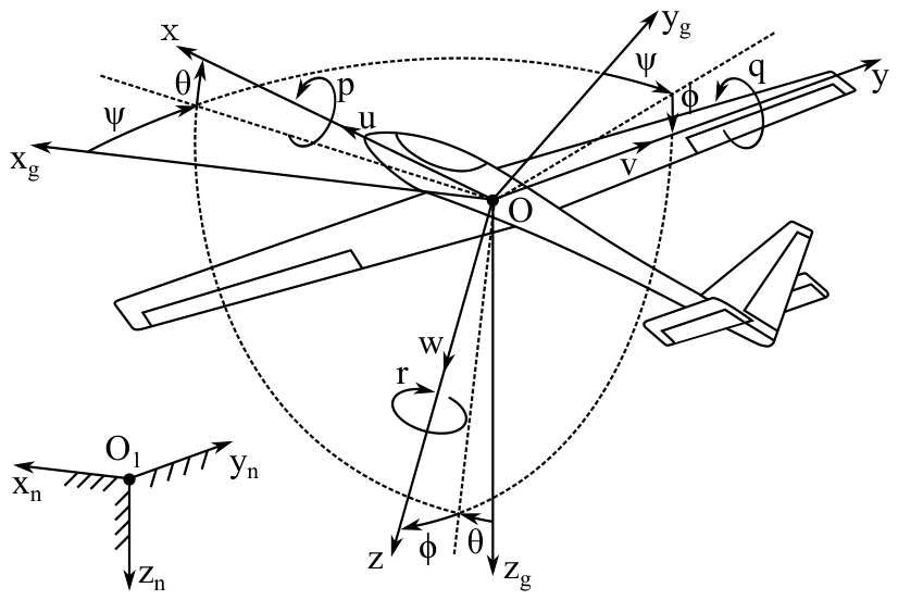
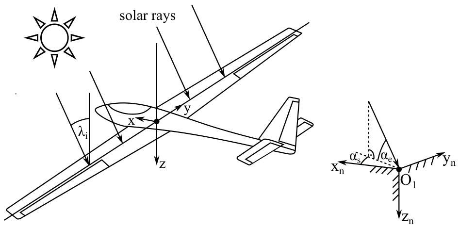
The UAV motion was described in a vehicle-carried body axes system $Oxyz$ shown in Figure 1. The longitudinal axis $Ox$ lies in the symmetry plane, is parallel to the mean aerodynamic chord and points toward the aircraft nose. The lateral axis $Oy$ is directed toward the right wing and points outward, whereas the vertical axis $Oz$ completes the right-handed reference system and points downward. The origin of this axis system O is located at an arbitrary point of the aircraft that lies in its symmetry plane.

As the equations of motion are given in the vehicle-carried reference frame, the change theorems used to develop dynamic equations of motion are as follows:

$$\dot{\mathsf{\Pi }}{|}_{loc}+\mathsf{\Omega }\times \mathsf{\Pi }=\mathbf{F}$$

(1)

$${\dot{\mathbf{K}}}_O{|}_{loc}+\mathsf{\Omega }\times {\mathbf{K}}_O+{\mathbf{V}}_O\times \mathsf{\Pi }={\mathbf{M}}_O$$

(2)

where $\mathsf{\Pi }$ and ${\mathbf{K}}_O$ are the linear and angular momenta, ${\mathbf{V}}_O=\left[uvw\right]$ and $\mathsf{\Omega }=\left[pqr\right]$ are the linear velocity and angular rates, $\mathbf{F}$ and ${\mathbf{M}}_O$ are total force and total moment with respect to point O, while $loc$ denotes the local derivative.

The aircraft was modelled as a rigid body, thus its momenta are:

$$\mathsf{\Pi }=m\left({\mathbf{V}}_O+\mathsf{\Omega }\times {\mathbf{r}}_C\right)$$

(3)

$${\mathbf{K}}_O={\mathbf{I}}_O\mathsf{\Omega }+{\mathbf{r}}_C\times m{\mathbf{V}}_O$$

(4)

where m denotes mass, $\mathbf{I}$ is the inertia matrix, in which $I_{xy}=I_{yz}=0$ due to aircraft vertical symmetry in terms of geometry and mass, while ${\mathbf{r}}_C$ is the centre of gravity offset. As in the study, there was no payload release, and the UAV used an electric motor; the mass was considered constant. A similar assumption was made for the inertia matrix, because inertia changes due to flight control deflections were considered negligible.

The external forces $\mathbf{F}$ and moment ${\mathbf{M}}_O$ vectors result from the interaction of aerodynamics, the propulsion system and gravity. To evaluate the aerodynamic characteristics, XFLR5 v 6.61 software was employed, combining a Vortex Lattice Method (VLM) formulation with a 3D surface panel method to determine both static and dynamic aerodynamic derivatives. The aerodynamic derivatives were extracted at a constant flight speed corresponding to the designed mission velocity and modelled as:

$$\begin{array}{c}{C}_D=C_{D_0}+C_{D_1}\alpha +C_{D_2}{\alpha }^2+C_{D_{{\delta }_E}}{\delta }_E\hfill \\ C_Y=C_{Y_0}+C_{Y_{\beta }}\beta +C_{Y_p}{p}^{*}+C_{Y_r}{r}^{*}+C_{Y_{{\delta }_A}}{\delta }_A+C_{Y_{{\delta }_R}}{\delta }_R\hfill \\ C_L=C_{L_0}+C_{L_{\alpha }}\alpha +C_{L_q}{q}^{*}+C_{L_{{\delta }_E}}{\delta }_E\hfill \\ C_l=C_{l_0}+C_{l_{\beta }}\beta +C_{l_p}{p}^{*}+C_{l_r}{r}^{*}+C_{l_{{\delta }_A}}{\delta }_A+C_{l_{{\delta }_R}}{\delta }_R\hfill \\ C_m=C_{m_0}+C_{m_{\alpha }}\alpha +C_{m_q}{q}^{*}+C_{m_{{\delta }_E}}{\delta }_E\hfill \\ C_n=C_{n_0}+C_{n_{\beta }}\beta +C_{n_p}{p}^{*}+C_{n_r}{r}^{*}+C_{n_{{\delta }_A}}{\delta }_A+C_{n_{{\delta }_R}}{\delta }_R\hfill \end{array}$$

(5)

where $C_L$, $C_Y$ and $C_D$ are lift, side and drag force aerodynamic coefficients, while $C_l$, $C_m$ and $C_n$ correspond to rolling, pitching and yawing moment aerodynamic coefficients, respectively. Angle of attack and sideslip angles are denoted as $\alpha$ and $\beta$, while $p^{*}=pb/2V_O$, $q^{*}=q\overline{c}/2V_O$ and $r^{*}=rb/2V_O$ are normalised roll p, pitch q and yaw r rates, where $\overline{c}$ is the mean aerodynamic chord, and b is the wingspan. Aileron, elevator and rudder control deflections are denoted as ${\delta }_A$, ${\delta }_E$ and ${\delta }_R$. The subscript zero stands for aerodynamic bias.

Since XFLR5 does not directly provide the drag polar coefficients $C_{D_1}$ and $C_{D_2}$, but instead outputs discrete drag coefficient values for a sequence of angles of attack at a constant free-stream velocity (Type-1 polar analysis), the corresponding drag polar was obtained by fitting an appropriate model to this data using the ordinary least squares method. Thus, the problem was formulated as:

$$\mathbf{Y}=\mathbf{X}\mathsf{\Theta }+\epsilon$$

(6)

where $\mathbf{Y}$ is the observed drag coefficients vector, and ${\mathbf{X}}_i=\left[1{\alpha }_i{\alpha }_i^2\right]$ represents the i-th row of the design matrix for a given angle of attack ${\alpha }_i$. The $\mathsf{\Theta }={\left[C_{D_0}{C}_{D_1}{C}_{D_2}\right]}^T$ is the unknown parameters vector, and $\epsilon$ denotes the residual error. The parameters were estimated as:

$$\widehat{\mathsf{\Theta }}={\left({\mathbf{X}}^T\mathbf{X}\right)}^{-1}{\mathbf{X}}^T\mathbf{Y}$$

(7)

The aerodynamic force and moment in XFLR5 are given in the stability reference frame as ${\mathbf{F}}_a=[-\overline{q}S{C}_D\overline{q}S{C}_Y-\overline{q}S{C}_L]$ and ${\mathbf{M}}_a=\left[\overline{q}Sb{C}_l\overline{q}S\overline{c}{C}_m\overline{q}Sb{C}_n\right]$, where S is the wing area, $\overline{c}$ and b are the mean aerodynamic chord and wingspan, respectively, and $\overline{q}=0.5\rho V_O^2$ is the dynamic pressure, with $\rho$ denoting air density. These vectors were subsequently transformed into the body axes.

The gravitational acceleration $g_0$ was computed using the WGS-84 Earth model [22], accounting for the aircraft’s geographic latitude and flight altitude. Since the aircraft is not intended to operate in the vicinity of a 90 deg pitch angle (avoiding the gimbal lock singularity), the gravity force in the body axes system, ${\mathbf{F}}_g$, was determined using the rotation matrix ${\mathbf{R}}_{BE}$ (from Earth-fixed to body axes) such that ${\mathbf{F}}_g=m{\mathbf{R}}_{BE}{[0,0,g_0]}^T$. The transformation matrix ${\mathbf{R}}_{BE}$ is defined as:

$${\mathbf{R}}_{BE}=\left[\begin{array}{ccc}1& 0& 0\\ 0& cos\varphi & sin\varphi \\ 0& -sin\varphi & cos\varphi \end{array}\right]\left[\begin{array}{ccc}cos\theta & 0& -sin\theta \\ 0& 1& 0\\ sin\theta & 0& cos\theta \end{array}\right]\left[\begin{array}{ccc}cos\psi & sin\psi & 0\\ -sin\psi & cos\psi & 0\\ 0& 0& 1\end{array}\right]$$

(8)

where $\varphi$, $\theta$, $\psi$ are Euler angles (roll, pitch and yaw angles) defined according to the Tait–Bryan convention. As the centre of gravity location was fixed, the gravitational moment was ${\mathbf{M}}_g={\mathbf{r}}_C\times {\mathbf{F}}_g$.

The total thrust T produced by the propulsion system was determined using the non-dimensional thrust coefficient $C_T$, derived from the propeller’s aerodynamic characteristics:

$$T=\rho n^2{D}^4{C}_T(V_0,\omega )$$

(9)

where $\omega$ denotes the rotational speed of the engine in revolutions per minute ($n=\omega /60$), while D is the propeller diameter.

To evaluate the total propulsion power consumption $P_P$, the mechanical power required to rotate the propeller was derived from the power coefficient $C_P$ and adjusted to account for the losses within the electronic speed controller (ESC) and the electric motor:

$$P_P={\displaystyle \frac{\rho n^3{D}^5{C}_P(V_0,\omega )}{{\eta }_{motor}{\eta }_{ESC}}}$$

(10)

where ${\eta }_{motor}$ and ${\eta }_{ESC}$ are motor and ESC efficiencies, respectively.

Thrust and power coefficients were evaluated for a fixed-pitch 12x5.5 propeller using the empirical formulas [23]:

$$\begin{array}{cc}\hfill C_T& =0.02791-0.06543J+0.11867{\beta }_p+0.27334{\beta }_p^2-0.28852{\beta }_p^3-0.23504J^2+\hfill \\ \hfill & +0.02104J^3+0.18677{\beta }_p{J}^2\hfill \\ \hfill C_P& =0.01813+0.00343J-0.06218{\beta }_p+0.35712{\beta }_p^2-0.23774{\beta }_p^3-0.1235J^2+\hfill \\ & +0.07549{\beta }_{p}J\hfill \end{array}$$

(11)

where $J=V/\left(nD\right)$ and ${\beta }_p=k_p/D$ are the advance and pitch ratios, with $k_p$ denoting propeller pitch.

The thrust vector ${\mathbf{F}}_T=\left[T00\right]$ was assumed to lie within the aircraft plane of symmetry, parallel to the longitudinal axis. However, since the thrust line did not pass through the origin of the body-fixed coordinate system O, it generated an additional propulsion moment. Furthermore, a gyroscopic effect produced by the rotating masses of the motor and the propeller was included, and thus the overall propulsion moment is:

$${\mathbf{M}}_P={\mathbf{r}}_T\times {\mathbf{F}}_T+\mathsf{\Omega }\times \left(I_{eng}{\omega }_p\right)$$

(12)

where ${\omega }_p={[\omega ·2\pi /6000]}^T$ is the angular velocity of the propeller in the vehicle-carried frame, ${\mathbf{r}}_T$ denotes the thrust force offset, while $I_{eng}$ is the engine moment of inertia.

By substituting the total external forces $\mathbf{F}$ and moments ${\mathbf{M}}_O$ into the dynamic equations of motion, the time derivatives of the linear and angular velocity components in the body-fixed frame are obtained. Integrating these derivatives yields the instantaneous linear velocity ${\mathbf{V}}_O$ and angular rates $\mathsf{\Omega }$.

To determine the aircraft position and attitude relative to the Earth-fixed North-East-Down navigation frame (NED), these body-axis state variables must be transformed. The UAV’s geodetic position rates ${\dot{\mathbf{r}}}_n={\left[{\dot{x}}_n{\dot{y}}_n{\dot{z}}_n\right]}^T$ are calculated by transforming the body-fixed velocity ${\mathbf{V}}_O$ using the inverse rotation matrix ${\dot{\mathbf{r}}}_n={\mathbf{R}}_{BE}^{-1}{\mathbf{V}}_O$ and then integrated to obtain the position vector components.

Simultaneously, the attitude of the UAV, expressed by the Euler angles, is updated by transforming the angular rates from the vehicle-carried system to the navigation frame:

$$\begin{array}{c}\dot{\varphi }=p+qsin\varphi tan\theta +rcos\varphi tan\theta \\ \dot{\theta }=qcos\varphi -rsin\varphi \\ \dot{\psi }=qsin\varphi sec\theta +rcos\varphi sec\theta \end{array}$$

(13)

In addition to the state variables, the flow angles are determined from linear velocity ${\mathbf{V}}_O$ components. Angle of attack $\alpha =arctan(w/u)$ and the sideslip angle $\beta =arctan(v/\sqrt{u^2+w^2})$ complete the set of kinematic and dynamic relations that describe the aircraft motion.

At the trim point, the aircraft model was in steady, straight, symmetric flight; thus, the total forces and moments were assumed to be zero. To determine the flight control inputs that satisfy this condition, only the longitudinal motion was analysed, with the gyroscopic moment set to zero (consistent with the trim condition ${\mathsf{\Omega }}_0=\mathbf{0}$). The resulting nonlinear set of equations was solved using the Levenberg–Marquardt algorithm. In addition to the trimmed elevator deflection ${{\delta }_E}_0$ and engine speed ${\omega }_0$, the pitch angle ${\theta }_0$ was also treated as a design variable.

To ensure the numerical framework is grounded in realistic engineering limits, the UAV geometry is based on the Multiplex Cularis aircraft; thus, the resulting aerodynamic characteristics and dynamic properties are consistent with the typical ranges expected for this class of UAVs and align with baseline physical intuition. This configuration serves the primary objective of the framework, which focuses on delivering a generic, flexible stochastic tool for mission feasibility assessment rather than replicating a specific aircraft.

The propulsion subsystem uncertainty was quantified using the empirical formulas derived in [23], which provide an average relative error and a standard deviation to describe the model’s performance. When applied to the propeller model used in this work, with speeds up to 30 m/s at 5000 RPM, the average power coefficient model error is 1.90% with a standard deviation of 1.43%. At the analysed cruise speed, the expected error is 1.88%, ensuring that the mission energy evaluation remains within physical limits.

3. Control System

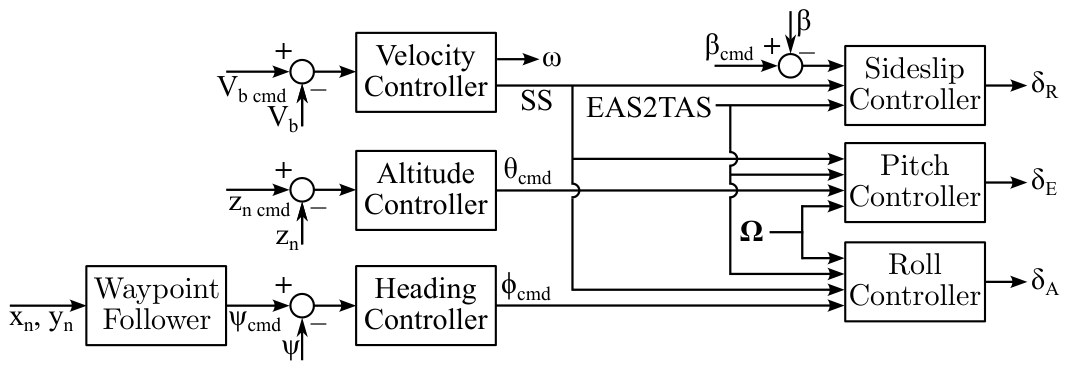
The flight control system of the solar-powered UAV is based on a hierarchical, cascaded architecture, as illustrated in Figure 2. This structure facilitates successive loop closure, where high-level navigation commands are progressively translated into actuator deflections. The architecture comprises the primary control branches: a velocity controller for thrust management, an altitude-and-pitch cascade for vertical path tracking and a lateral-directional suite that controls both heading and sideslip.

The UAV flight is managed by a cascaded control architecture with Pure Pursuit Waypoint Following algorithm [24], attitude and velocity controllers. The overall autopilot architecture schematic is presented in Figure 2.

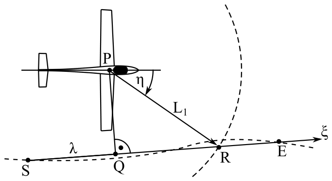
Guidance is handled by the outermost layer, which employs a Pure Pursuit Waypoint Following algorithm [24] to track a reference path defined by the mission plan. The geometric logic is shown in Figure 3.

In this approach, the aircraft tracks a virtual lookahead point R, which lies on a straight segment between the start S and end waypoints E and is updated in each step:

$$R=S+{\xi }_R{\mathbf{r}}_{SE}$$

(14)

where ${\xi }_R$ is a scalar parameter representing lookahead point normalised position along the $SE$ segment.

The lookahead point R position is located at an adaptive lookahead distance $L_1$ from the UAV, satisfying the following geometric constraint:

$$\parallel {\mathbf{r}}_{PS}+{\xi }_R{\mathbf{r}}_{SE}{\parallel }^2=L_1^2$$

(15)

The lookahead distance $L_1$ is adaptively scaled based on the current cross-track error to maintain numerical stability. Solving this equation with respect to ${\xi }_R$ yields two potential roots, and the maximum value is selected to ensure forward progress.

Once the lookahead point R is established, the desired heading angle ${\psi }_{cmd}$ is determined using the relative vector $PR$ horizontal components

$${\psi }_{cmd}=arctan\left({\displaystyle \frac{{\mathbf{r}}_{PR}·{\mathbf{e}}_y}{{\mathbf{r}}_{PR}·{\mathbf{e}}_x}}\right)$$

(16)

where ${\mathbf{e}}_x$ and ${\mathbf{e}}_y$ are the unit vectors in longitudinal- and side- directions, and · denotes the dot product.

The waypoint index is updated, and the line segment shifts to the next pair of coordinates if the UAV enters an acceptance radius $R_t$ around the end waypoint E ($\parallel {\mathbf{r}}_{PE}\parallel \le R_t$), or it passes the end point E. To verify whether the end waypoint E was passed, a non-dimensional projection parameter $\lambda$ is used to determine the progress along the $SE$ segment:

$$\lambda ={\displaystyle \frac{{\mathbf{r}}_{SP}·{\mathbf{r}}_{SE}}{\parallel {\mathbf{r}}_{SE}\parallel }}$$

(17)

and the switching triggers waypoint update when $\lambda >1$.

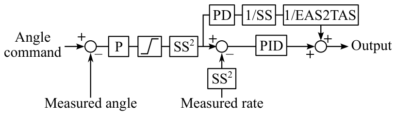
As mentioned, the stabilisation and command tracking are performed by a multi-loop structure. The attitude controllers for roll ($\varphi$) and pitch ($\theta$) are implemented as shown in Figure 4, using a cascaded topology with proportional gain in the outer loop and PID controller in the inner loop. To improve transient response, a PD feed-forward path is incorporated with Equivalent Airspeed to True Airspeed ($EAS2TAS$) correction to compensate for varying atmospheric density with altitude. To ensure consistent performance across the flight envelope, speed scaling $SS$ is also applied.

The sideslip controller actively maintains a zero-sideslip condition (${\beta }_{cmd}=0^{°}$), keeping the airframe aligned with the flow during the long straight-line segments. It utilises a single-loop with PID/PD-FF architecture as in the roll and pitch channels; unlike the attitude channels, it does not include an outer proportional block. The velocity controller is intended to hold a constant velocity $V_0$. The current and trimmed flight velocities are used to determine speed scaling $SS=V_0/V$.

The altitude and heading are managed by standalone PID controllers. Each PD or PID module in the autopilot block employs derivative filters to mitigate sensor noise, anti-windup clamping logic and saturation to respect physical limits. The controllers were tuned assuming the UAV would hold a given speed and altitude, fulfilling the pixel-resolution and Ground Sampling Distance requirements of remote sensing and photogrammetric monitoring missions. While horizontal waypoint navigation is managed by a Pure Pursuit algorithm, the altitude control loop is optimised for disturbance rejection at a fixed operating point to ensure maximum steady-state stability, rather than altitude tracking.

Furthermore, the control commands adjusted by trimmed values are passed through rate limiters to account for servo dynamics, followed by first-order transfer functions and final saturation blocks to model the actuator response and mechanical constraints.

4. Environment

4.1. Irradiance

The primary energy harvesting component of a solar-powered UAV is the wing, owing to its significant surface area and predominantly horizontal orientation during cruise. While control surfaces and airframe curvature limit the effective installation area, the wing’s planar geometry facilitates high-efficiency PV integration. The total solar irradiance incident on the wing surface, $I_T$, is composed of beam ($I_b$), diffuse ($I_d$) and ground-reflected ($I_r$) components:

$$I_T=I_b+I_d+I_r$$

(18)

The effective energy harvested depends on the solar incident angle ${\lambda }_i$ relative to the wing’s surface normal and the aircraft’s spatial orientation.

The irradiance components are projected as:

$$I_b=\left\{\begin{array}{cc}{\widehat{I}}_{b,n}cos{\lambda }_i& cos{\lambda }_i\ge 0\\ 0& cos{\lambda }_i<0\end{array}\right.$$

(19)

$$I_d={\widehat{I}}_{d,h}{cos}^2{\displaystyle \frac{{\lambda }_t}{2}}$$

(20)

In this framework, ${\widehat{I}}_{b,n}$ and ${\widehat{I}}_{d,h}$ denote the adjusted beam normal and horizontal diffuse irradiance components that are augmented to reflect the local irradiance conditions bias $\nu$ and variability $\sigma$:

$$\begin{array}{c}{\widehat{I}}_{b,n}=I_{b,n}+{\nu }_b+{\sigma }_b{\xi }_b\hfill \\ {\widehat{I}}_{d,h}=I_{d,h}+{\nu }_d+{\sigma }_d(0.5{\xi }_d-0.5{\xi }_b)\hfill \end{array}$$

(21)

where ${\xi }_b,{\xi }_d\sim \mathcal{N}(0,1)$ denote independent standard Gaussian random variables with the coupled stochastic term used to emulate the anti-correlated behaviour between DNI and DHI variations.

The solar incident angle ${\lambda }_i$, shown in Figure 5, is derived by transforming the solar position vector into the aircraft body-fixed frame:

$$\begin{array}{cc}{\lambda }_i=\hfill & \arccos (-\cos {\alpha }_e\cos {\alpha }_s(\sin \varphi \sin \psi +\cos \varphi \sin \theta \cos \psi )+\hfill \\ \hfill & \cos {\alpha }_e\sin {\alpha }_s(\sin \varphi \cos \psi -\cos \varphi \sin \theta \sin \psi )+\sin {\alpha }_e\cos \varphi \cos \theta )\hfill \end{array}$$

(22)

Simultaneously, the wing tilt angle ${\lambda }_t$ is given by:

$${\lambda }_t=\arccos \left(\cos \varphi \cos \theta \right)$$

(23)

The solar position, defined by the altitude angle ${\alpha }_e$ and azimuth angle ${\alpha }_s$, varies according to the observer’s latitude L, the solar declination ${\delta }_s$ and the solar hour angle $h_s$:

$$\begin{array}{c}{\alpha }_e=\arcsin \left(\sin {\delta }_s\sin L+\cos {\delta }_s\cos L\cos h_s\right)\\ {\alpha }_s=\arccos \left((\sin {\delta }_s\cos L-\cos {\delta }_s\sin L\cos h_s)/\cos {\alpha }_e\right)\end{array}$$

(24)

with ${\alpha }_s=360-{\alpha }_s$ when $h_s>0$.

Accounting for the Earth’s axial tilt relative to the ecliptic plane, the solar declination ${\delta }_s$ is approximated as a function of the day of the year n:

$${\delta }_s=23.45sin{\displaystyle \frac{360(284+n)}{365}}$$

(25)

The solar hour angle $h_s$, quantifying the Sun’s angular displacement from the local meridian, is derived from the solar time $ST$:

$$h_s=15(LST+ET-4(l_{ST}-l_{local})-12)$$

(26)

where $l_{local}$ denotes the local longitude, $l_{ST}$ is the standard time meridian, while the Equation of Time ($ET$) accounting for Earth’s orbital irregularities is approximated as:

$$\begin{array}{cc}ET=\hfill & 229.2(0.000075+0.001868cosB-0.032077sinB\hfill \\ & -0.014615cos2B-0.04089sin2B)\hfill \end{array}$$

(27)

where $B=360(n-1)/365$.

To estimate the direct normal irradiance $I_{b,n}$ and diffuse horizontal irradiance $I_{d,h}$, a locally-adjusted ASHRAE clear-sky model is used. In the baseline formulation, the extraterrestrial normal irradiance I is calculated by adjusting the solar constant $I_0=1353{\mathrm{W}/\mathrm{m}}^2$ for the Earth’s orbital eccentricity [25]:

$$I=I_0\left(1+0.033cos\left({\displaystyle \frac{360n}{365}}\right)\right)$$

(28)

where n is the day of the year. Atmospheric attenuation is modelled via the Beer–Bouguer–Lambert law:

$$\begin{array}{c}{I}_{b,n}=I{e}^{-{\tau }_b{m}_s^b}\\ I_{d,h}=I{e}^{-{\tau }_d{m}_s^d}\end{array}$$

(29)

where ${\tau }_b$ and ${\tau }_d$ are the beam and diffuse pseudo-optical depths, which represent the attenuation due to absorption and scattering under prevailing local atmospheric conditions and are given for the 21st day of each month and a specified location. The air mass ratio $m_s$, which accounts for the dimensionless path length of sunlight traversing the atmosphere, is given as [26]:

$$m_s={\displaystyle \frac{1}{sin{\alpha }_e+0.50572{(6.07995+{\alpha }_e)}^{-1.6364}}}$$

(30)

while the air mass exponents are found from empirical formulas [27]:

$$\begin{array}{c}b=1.219-0.043{\tau }_b-0.151{\tau }_d-0.204{\tau }_b{\tau }_d\\ d=0.202+0.520{\tau }_b-0.007{\tau }_d-0.357{\tau }_b{\tau }_d\end{array}$$

(31)

Finally, the ground reflected irradiance incident on the wing surface is expressed by:

$$I_r={\alpha }_r\left({\widehat{I}}_{b,n}sin{\alpha }_e+{\widehat{I}}_{d,h}\right){sin}^2{\displaystyle \frac{{\lambda }_t}{2}}$$

(32)

where ${\alpha }_r$ is the ground reflectance coefficient [28]:

$${\alpha }_r={\alpha }_0{\displaystyle \frac{1+d_r}{1+2d_{r}cos{\theta }_z}}$$

(33)

with ${\alpha }_0$ representing the baseline albedo, $d_r$ accounting for surface roughness and ${\theta }_z=90-{\alpha }_e$ denoting the zenith angle.

4.2. Cloud Cover

To evaluate UAV operational feasibility in high-variability climates, the deterministic clear-sky model is augmented with a stochastic cloudiness framework. This model simulates transitions between clear-sky and cloudy-sky states by assigning a time-varying opacity to the atmosphere and applying signal smoothing to achieve physically realistic cloud edges.

The cloudiness is represented as a semi-Markov process operating on a discrete state, where 0 denotes cloudy conditions, while 1 represents clear-sky. In contrast to a classical Markov process, which exhibits the memoryless property, the proposed semi-Markov model incorporates the dwell time in the current state $t_{state}$. The transition mechanism is governed by system inertia, which prevents a state change before a minimum dwell time, $t_{min}$, has elapsed. Once this threshold is exceeded, the process regains its memoryless characteristics, and the transition probability becomes constant for each subsequent time step.

The cloud profile is generated sequentially at a 10 min resolution $\Delta t$. At each time instance, the model evaluates the transition condition based on the desired mean state duration. The transition probabilities are defined as follows:

$$P(i\to j)={\displaystyle \frac{\Delta t}{t_i-t_{min}}},i\ne j,i,j\in \{0,1\}$$

(34)

where $t_0$ and $t_1$ are the desired mean state duration for the cloudy and clear-sky states, respectively.

When the system enters a cloudy state, the cloud opacity O is determined via a two-stage stochastic process:

$$O=\left\{\begin{array}{cc}1\hfill & {\xi }_1<p_{op}\hfill \\ 0.2+0.6{\xi }_2\hfill & {\xi }_1\ge p_{op}\hfill \end{array}\right.$$

(35)

where ${\xi }_1,{\xi }_2\sim \mathcal{U}(0,1)$ denote uniformly distributed random variables, while $p_{op}$ is the probability of encountering a fully opaque cloud. Conversely, for the clear-sky state, the opacity is defined as $O=0$.

To simulate the physical phenomena of cloud overlap and dissipation, the opacity vector undergoes a two-stage smoothing process. First, a moving average filter with a fixed window width $w=\lfloor t_{ramp}/\Delta t\rceil$ is applied for initial smoothing to obtain the intermediate profile $\tilde{O}$, with $t_{ramp}$ denoting the transition time between clear-sky and cloudy states.

To ensure a continuous and physically consistent transition, this intermediate profile is further refined. Subsequently, a zero-phase (forward–backward) first-order recursive low-pass filter is applied to produce a smooth, realistic character to the cloud edges, simulating the gradual entry and exit of the solar disk behind a cloud layer:

$${\widehat{O}}_i=(1-{\alpha }_O){\widehat{O}}_{i-1}+{\alpha }_O{\tilde{O}}_i$$

(36)

where $\widehat{O}$ represents the smoothed opacity vector, and the filter coefficient is based on the desired sampling and transition time ${\alpha }_O=\Delta t/t_{ramp}$.

By utilising the smoothed opacity mask $\widehat{O}$, the modifiers for DNI ($k_{DNI}$) and DHI ($k_{DHI}$) are evaluated to account for the dual impact of cloudiness on solar radiation components. Specifically, the clouds attenuate the direct beam while simultaneously increasing the diffuse fraction due to multiple scattering phenomena:

$$\begin{array}{c}{k}_{DNI}=1-\widehat{O}(1-k_{min,DNI})\\ k_{DHI}=1+\widehat{O}(k_{max,DHI}-1)\end{array}$$

(37)

where $k_{min,DNI}$ represents the minimum transmittance limit of the direct beam under peak opacity, while $k_{max,DHI}$ denotes the corresponding maximum diffuse enhancement factor. These parameters define the model’s dynamic range, anchoring the stochastic fluctuations between the clear-sky baseline and the physically observed overcast extremes.

To align the generated stochastic profile with the simulation time steps, the cloud-induced modifiers $k_{DNI}$ and $k_{DHI}$, initially obtained at a 10 min resolution, are linearly interpolated for any specific Local Standard Time ($LST$). Finally, these interpolated factors are multiplied by the clear-sky beam normal ${\widehat{I}}_{b,n}$ and diffuse horizontal ${\widehat{I}}_{d,h}$ components to produce the cloud-corrected irradiance.

The baseline parameters of the proposed semi-Markov framework were selected to mirror localised long-term meteorological profiles, ensuring high statistical convergence of cloudiness distributions for the Warsaw region. Although the resulting configuration accurately captures these high-fidelity operational risk trends, the mathematical framework itself remains inherently generic. Thus, deploying it to an entirely different climate class is possible, but would require dedicated parameter re-validation under new constraints.

The proposed stochastic framework is designed as a modular engine capable of ingesting various clear-sky irradiance formulations based on the ASHRAE model to isolate and minimise local atmospheric uncertainty. As the solar UAV continuously moves relative to cloud formations, it inherently experiences high-frequency temporal dynamics and sudden irradiance fluctuations when it enters and exits localised cloud shadows. Thus, the environment model intentionally uses sequential, continuous cloud cover profiles rather than step-type classifications to capture real-time operational risk and energy storage volatility that spatially or temporally averaged discrete baselines fail to replicate.

4.3. Thermodynamic Parameters

To complement the irradiance formulation, the framework incorporates a dynamic temperature model and the International Standard Atmosphere profile [29]. The ground-level ambient temperature $T_a$ is estimated using the sinusoidal approximation by Parton and Logan [30], which accounts for the diurnal thermal cycle:

$$T_a=T_{min}+(T_{max}-T_{min})sin\left({\displaystyle \frac{\pi }{2}}{\displaystyle \frac{t-t_m}{t_n-t_m}}\right)$$

(38)

where $T_{min}$ and $T_{max}$ are the daily extremes recorded at times $t_m$ and $t_n$.

Height-dependent variations in thermodynamic parameters within the troposphere are introduced by converting the geometric altitude into geopotential altitude:

$$h_{geo}={\displaystyle \frac{h{R}_0}{h+R_0}}$$

(39)

with $R_0$ denoting the Earth’s reference radius.

The temperature T at a given geopotential altitude is determined by the lapse rate $\gamma$:

$$T=T_0-h_{geo}\gamma$$

(40)

where $T_0$ is the reference temperature at sea level.

Consequently, the atmospheric pressure p is calculated as:

$$p=p_0{\left(1-{\displaystyle \frac{h_{geo}\gamma }{T_0}}\right)}^{{\displaystyle \frac{g_0}{R\gamma }}}$$

(41)

with $p_0$ representing the standard sea-level pressure, $g_0$ the standard gravity at 45°32’33” latitude and sea level, while R is the air specific gas constant.

Finally, the air density $\rho$ is derived from the ideal gas law:

$$\rho ={\displaystyle \frac{p}{RT}}$$

(42)

4.4. Geodetic Gravity Formulation

The environmental model is completed by a gravity formulation dependent on both altitude and latitude, following the WGS84 Earth model [22]:

$$g=g_0{\displaystyle \frac{1+k{sin}^{2}L}{\sqrt{1-e^2{sin}^{2}L}}}{\left({\displaystyle \frac{R_e}{R_e+h}}\right)}^2$$

(43)

where $R_e$ is the Earth radius:

$$R_e={\displaystyle \frac{ab}{\sqrt{a^2{sin}^{2}L+b^2{cos}^{2}L}}}$$

(44)

with a and b representing the Earth ellipsoid major and minor axes, while k and e are the gravity formula constant and eccentricity.

To maintain geodetic accuracy, the model accounts for the UAV’s latitudinal displacement. For the incremental distances covered between simulation steps, a local flat-plane approximation is employed, where the northward displacement $x_n$ relates linearly to the change in latitude $\Delta L$:

$$\Delta L={\displaystyle \frac{x_n}{R_m}}$$

(45)

with the meridian radius of curvature $R_m$:

$$R_m={\displaystyle \frac{a(1-e^2)}{{(1-e^2{sin}^{2}L)}^{3/2}}}$$

(46)

5. PV System and Li-Ion Battery

The instantaneous available power $P_{PV}$ generated by the solar array is determined by the total incident irradiance $I_T$ on the wing surface and the overall efficiency of the energy conversion chain:

$$P_{PV}={\eta }_{\mathrm{c},\mathrm{a}}{\eta }_{\mathrm{c},\mathrm{T}}{S}_{PV}{I}_T-P_P-P_{\mathrm{sub}}$$

(47)

where $S_{PV}$ is the solar cell area, $P_P$ denotes the propulsion power, $P_{sub}$ represents the power consumption of the onboard systems, while ${\eta }_{c,a}$ accounts for the airfoil camber efficiency, reflecting the reduction in effective area due to the wing’s curvature. The temperature-dependent efficiency of the PV cells ${\eta }_{c,T}$ is modelled as [31]:

$${\eta }_{c,T}={\eta }_{c,ref}(1-{\beta }_{ref}(T_c-T_{ref}))$$

(48)

where ${\eta }_{c,ref}$ is the cell reference efficiency, ${\beta }_{ref}$ represents the temperature efficiency correction, while $T_c$ and $T_{ref}$ are cell and reference temperatures, respectively. To account for convective cooling during flight, the cell temperature $T_c$ is estimated using an analogous relation of Nusselt–Jürges [32]:

$$T_c=T_a+{\displaystyle \frac{0.25}{5.7+3.8V_O}}{I}_T$$

(49)

As the PV systems utilise a Maximum Power Point Tracking (MPPT) unit, its efficiency is included when evaluating the power delivered to the battery system $P=P_{PV}{\eta }_{MPPT}$:

$${\eta }_{MPPT}={\displaystyle \frac{P_{PV}-P_{loss}}{P_{PV}}}$$

(50)

where the MPPT power losses $P_{loss}$ are represented by a polynomial capturing the system’s self-consumption $a_{MPPT}$, voltage drop $b_{MPPT}$ and resistive dissipation $c_{MPPT}$ [33]:

$$P_{loss}=a_{MPPT}+b_{MPPT}{P}_{PV}+c_{MPPT}{P}_{PV}^2$$

(51)

The battery management system controls the current flow based on the net power P and its voltage V. The commanded charging/discharging current $i_{cmd}$ is corrected for battery internal efficiency ${\eta }_{batt}$:

$$i_{cmd}={\displaystyle \frac{P}{V}}{\eta }_{batt}$$

(52)

with ${\eta }_{batt}={\eta }_{ch}$ when the battery is charged and ${\eta }_{batt}=1/{\eta }_{ch}$ when it is discharged.

To prevent overcharging, a Constant Current-Constant Voltage (CC-CV) control logic was implemented. When the battery voltage reaches its maximum threshold $V_{max}$ during charging, a proportional-integral (PI) controller modulates the battery current i:

$$i=\left(K_p+{\displaystyle \frac{K_i}{s}}\right)(V_{max}-V)$$

(53)

where $K_p$ and $K_i$ are the PI controller parameters. Otherwise, the current follows the target value $i=i_{cmd}$.

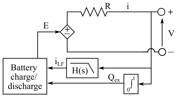
The Li-Ion battery is represented by an equivalent circuit model, as illustrated in Figure 6. To accurately capture the non-linear discharge and charge characteristics, the terminal voltage V is determined using a Tremblay battery model [34,35]. This formulation accounts for the different electrochemical dynamics during charging ($i>0$) and discharging ($i<0$) states:

$$V=\left\{\begin{array}{cc}{E}_0-K\left({\displaystyle \frac{Q}{Q_{ex}+0.1Q}}{i}_{LF}+{\displaystyle \frac{Q}{Q-Q_{ex}}}{Q}_{ex}\right)+Aexp(-B{Q}_{ex})-i{R}_b\hfill & i>0\hfill \\ E_0-K\left({\displaystyle \frac{Q}{Q-Q_{ex}}}{i}_{LF}+{\displaystyle \frac{Q}{Q-Q_{ex}}}{Q}_{ex}\right)+Aexp(-B{Q}_{ex})-i{R}_b\hfill & i<0\hfill \end{array}\right.$$

(54)

where $E_0$ is the constant voltage, $R_b$ represents the internal resistance, K is the polarisation constant, A and B are the exponential voltage and exponential capacity constants, while Q and $Q_{ex}={\int }_0^{t}i\left(\tau \right)d\tau$ denote the maximum and extracted capacities, respectively. The battery parameters follow the generic and scalable modelling philosophy used for the UAV platform. To ensure realistic electrochemical behaviour a Li-Ion battery with an 11.1 V nominal voltage and 3.195 Ah maximum capacity was used as a reference and the specific constants, which capture the macro-characteristics of this cell class, were established as: $E_0$ = 12.036 V, K = 0.03438 V, A = 0.58448 V, B = 20.354 Ah⁻¹ and $R_b$ = 0.037 $\mathsf{\Omega }$.

To accurately reflect the electrochemical lag in battery transient response, the model incorporates a filtered current component $i_{LF}=H\left(s\right)i$ representing the low-order dynamics of the polarisation voltage. This ensures that the open-circuit voltage does not respond instantaneously to step changes in power demand:

$$H\left(s\right)={\displaystyle \frac{1}{T_{batt}s+1}}$$

(55)

Finally, the battery State of Charge $SOC$ is updated by integrating the current flow:

$$SOC=1-{\displaystyle \frac{Q_{ex}}{Q}}{\lambda }_{batt}$$

(56)

where ${\lambda }_b$ accounts for capacity degradation and aging effects.

6. Hardware and Simulation Setup

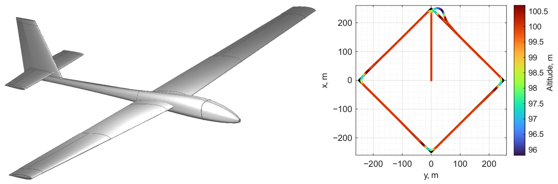
The fixed-wing UAV platform used in this study (Figure 7) is based on the electric-powered Multiplex Cularis with integrated monocrystalline solar cells on the upper wing surface. The modelled aircraft had a wingspan of 2.6 m, a total length of 1.14 m and a total wing area of 0.42 m², with a mean aerodynamic chord of 0.163 m. The energy subsystem incorporated a 3.195 Ah 3S1P LiPo battery. The initial State of Charge (SOC) was set to 70% to represent a realistic operational state at the onset of the monitoring phase, accounting for the energy previously expended during take-off and climb while preserving the battery life by not charging it above the safety threshold. The mission was programmed to terminate at 15% SOC, serving as a mandatory safety buffer to ensure sufficient power for landing procedures.

During the mission, the aircraft maintained a constant operational speed of 12.4 m/s at an altitude of 100 m. After an initial 250 m rectilinear northbound segment and a 135° eastward turn, the UAV executed a repetitive diamond-shaped infrastructure inspection. This pattern consisted of four segments, each 250 m in length, forming a closed square loop rotated by 45° relative to the initial path, as shown in Figure 7.

While dynamic trajectory adaptation can significantly enhance energy harvesting in solar aviation, practical infrastructure monitoring and tactical surveillance missions often impose rigid operational boundaries. In such scenarios, the flight path is invariant and strictly dictated by the spatial location of the monitored assets. Consequently, the predetermined trajectory investigated in this study represents a conservative operational constraint; since the UAV is restricted from actively adjusting its course to avoid cloud cover or optimise the solar incidence angle, this approach provides a rigorous assessment of mission feasibility under real-world operational profiles.

To evaluate the flight time change due to atmospheric uncertainty and solar system design, a large-scale sensitivity analysis was conducted, comprising 920,506 individual simulations summarised in

Table 1. Scenarios summary.

Scenario Group	Type	Scenario-Specific Design Parameters
Clear-sky	Y	$\nu ={\nu }_0+{\alpha }_{\sigma }\sigma ,{\alpha }_{\sigma }\in [-3:1:3]$
Realistic atmosphere	D	$(t_0,t_1)\in \{(x,1.0),(1.0,x)\},x\in \{1.0,1.5,2.0\}$
Variable atmosphere	D	$t_0=t_1\in \{0.5,1.0,1.5,3.0\}$
Extreme atmosphere	D	$(t_0,t_1)\in \{(x,0.5),(0.5,x)\},x\in \{0.5,3.0,5.0\}$
Cloud cover type	D	$\mathbf{k}\in \left\{\right(k,2-k)\mid k\in \{0.2,0.6,0.8\left\}\right\}\cup \left\{\right(0.1,2.2\left)\right\}$
Solar area and	Y	$S_{PV}={\alpha }_{S}S,{\alpha }_S\in [0.2:0.1:0.7]$, $Q\in$ {3.195, 6.390}
battery capacity	D
Battery and PV	D	${\alpha }_{b}Q$, ${\alpha }_b^{-1}\{B,K,R_b\}$, ${\alpha }_b\sim \mathcal{U}(0.9,1.1)$
system uncertainty	D	${\alpha }_{PV}{\eta }_{c,ref}$, ${\alpha }_{PV}\sim \mathcal{U}(0.9,1.1)$
Clear-sky	Y	$\nu ={\nu }_0+{\alpha }_{\sigma }\sigma ,{\alpha }_{\sigma }\in [-3:1:3]$
$S_{PV}=0.6S$
Realistic atmosphere,	D	$(t_0,t_1)\in \{(x,1.0),(1.0,x)\},x\in \{1.0,1.5,2.0\}$, Q = 3.195
$S_{PV}=0.6S$	D	$(t_0,t_1)\in \{(x,1.0),(1.0,x)\},x\in \{1.0,1.5,2.0\}$, Q = 6.390

Symbols: Y—Yearly (clear-sky), D—Daily (cloud cover included); default values: ${\nu }_0=({\nu }_{DNI},{\nu }_{DHI})=(50;-10)$ W/m², $\sigma =({\sigma }_{DNI},{\sigma }_{DHI})=(40;5)$ W/m², ${\alpha }_{\sigma }=1$ (always DNI/DHI shared); $t_0$ = 1.0 h, $t_1$ = 1.5 h; $\mathbf{k}=(k_{DNI},k_{DHI})=(0.2,1.8)$; ${\alpha }_S$ = 0.3; Q = 3.195 Ah.

. These scenarios investigated the impact of irradiance-based variability, stochastic cloud-state transitions and solar-to-wing area ratios across two battery capacities, using Warsaw (all-year from sunrise to sunset or 15 July, start at 12:00 LST) as the representative Central European location. Aerodynamic coefficient uncertainties were excluded from the stochastic loop, as their impact is limited to a proportional shift in power consumption due to the repetitive flight pattern. The analysis was designed to highlight the influence of each investigated parameter on mission success.

To ensure computational efficiency for such an extensive dataset, a decoupled simulation strategy was implemented: the high-fidelity aircraft dynamics for the initial and repeating mission segments were pre-evaluated at 0.001 s step and stored. These parameters were then down-sampled to 0.1 s resolution and used as an input for the subsequent irradiance and energy-balance evaluations, where the initial segment was processed once and then followed by the looped repetitive cycle to simulate the full mission duration. This approach significantly reduced the required computational time while yielding negligible differences in flight time compared to fully coupled simulations.

The validity of this decoupled simulation strategy was rigorously verified against a high-fidelity, fully coupled flight dynamics model for a set of clear-sky scenarios. Due to the high bandwidth of the autopilot and the steady nature of the cruise flight, minor variations in flight parameters and power demands introduced a negligible difference in the final flight time, which did not exceed 1%, confirming that the 0.1 s sampling rate is sufficient to preserve accuracy. This error resulted from the discretisation during downsampling of the high-frequency state parameters and required power time histories (from a 0.001 s to a 0.1 s time step), which introduced minor discrepancies between these variables. Additionally, because the solar irradiance and battery models are non-linear, evaluating them directly at a coarser 0.1 s time step introduces a non-linear approximation error. Since the error magnitude is directly influenced by specific scenario inputs, such as solar irradiance (coverage area, cloud level, time, etc.), battery parameters, and specific operational constraints, the error varies across different setups. Therefore, it was evaluated across selected scenarios to assess its impact, which was consistently below 1%. Furthermore, because the mission is programmed to terminate immediately once the battery State of Charge drops to the 15% safety threshold, the UAV never operates in an energy-starved state within the simulation envelope. This operational boundary eliminates the need to simulate degraded flight dynamics below the threshold, making the decoupled approach both physically justified and computationally indispensable for the large-scale analysis.

All evaluations were performed on an HP Z4 G4 workstation running Windows 11 Pro. The hardware configuration featured an Intel Xeon W-2295 processor (18 physical cores, 3.00 GHz), 64 GB of DDR4 RAM (2933 MT/s), NVIDIA Quadro RTX 4000 GPU (8 GB) and an NVMe SSD. The evaluations were performed in MATLAB and Simulink (R2025a) using the Parallel Computing Toolbox to distribute the workload across physical cores.

7. Results

7.1. Clear-Sky Conditions

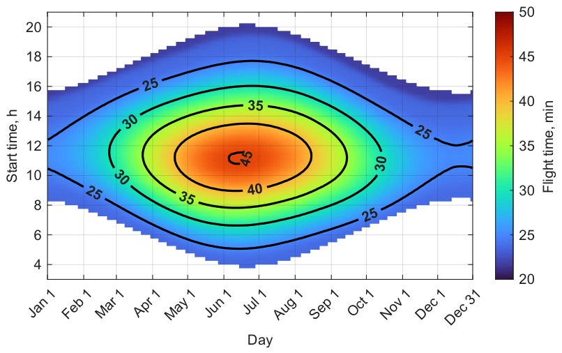
The flight time evaluated with a 15 min resolution from sunrise to sunset, utilising the median adjusted irradiance model for the default solar UAV configuration, is presented in Figure 8.

Under favourable weather conditions, the flight time can be doubled compared to a non-solar design (0:21:50). This benefit is prominent from late April to early August, but requires precise mission planning to capture the most energy-efficient part of the day, which occurs approximately within $\pm 1$ h from solar noon. The absolute maximum flight time was observed for a June 15 start at 11:15 (0:45:11). The flight duration was extended to 40 min in 9.33% instances, representing the upper performance limit under median clear-sky conditions.

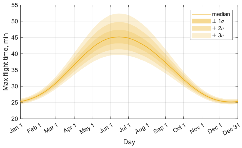
While the median model establishes the baseline performance, the atmospheric variability of the Central European climate introduces significant operational uncertainty. The maximum flight time limits for each day at various confidence intervals is shown in Figure 9.

It can be seen that the irradiance-based variability increases towards its summer peak and subsequently drops, while having approximately up to 10% impact during the late April to early August period. Specifically, at the June 15 peak, the maximum flight time in 68% of the cases ranges from 2.0 min (−4.5%) shorter to 2.2 (+4.8%) min longer operational windows compared to the nominal conditions. For 95.4% of the instances, this results in a broader span from 3.8 min (−8.5%) flight endurance reduction to 4.6 min (+10.1%) extension. In the most extreme scenarios captured within the 99.7% interval, the flight time can decrease up to 5.5 min (−12.2%) or increase up to 7.2 min (+15.9%). These demonstrate that even during the most solar-energy-dominant part of the year period radiation deficits can noticeably reduce the expected flight duration. This is further intensified when cloud cover influence is considered.

7.2. Cloud Cover Time

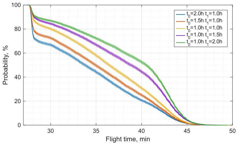
Evaluation of the UAV’s operational reliability requires analysing its performance assuming stochastically varying cloud cover. The probability of achieving a given flight time on 15 July (start at 12:00 LST) across realistic atmospheric regimes was evaluated using 10,000 Monte Carlo simulations and is shown in Figure 10, where the mean durations of the cloudy $t_0$ and clear-sky $t_1$ states were varied to simulate different weather forecasts.

A prominent physical feature visible across all scenarios is the distinct inflection point occurring approximately at 28 min, which is 6 min longer than for the battery-only flight and 15 min shorter than for the median clear-sky conditions. This indicates that even under a heavy overcast, the solar irradiance can be used to extend the flight time if the mission is carried out during the energy-efficient time period. Beyond this threshold, a sharp shift occurs, and the flight time extension becomes entirely dependent on stochastic solar harvesting. As the disparity between the clear-sky and cloudy state durations increases, the survival probability becomes highly non-linear and asymmetrical. When the cloud state dominates, the median flight time drops to approximately 34 min with a 50% probability. For the symmetrical baseline, this shifts to 36 min, whereas a sun-dominated forecast pushes the flight duration to 40 min. This demonstrates that the benefits of a sun-moderated regime far outweigh the penalties of equivalent cloud-dominated conditions, highlighting a positive sensitivity to clear-sky persistence. Furthermore, the 95% confidence intervals for each scenario remain highly consistent, with a narrow width.

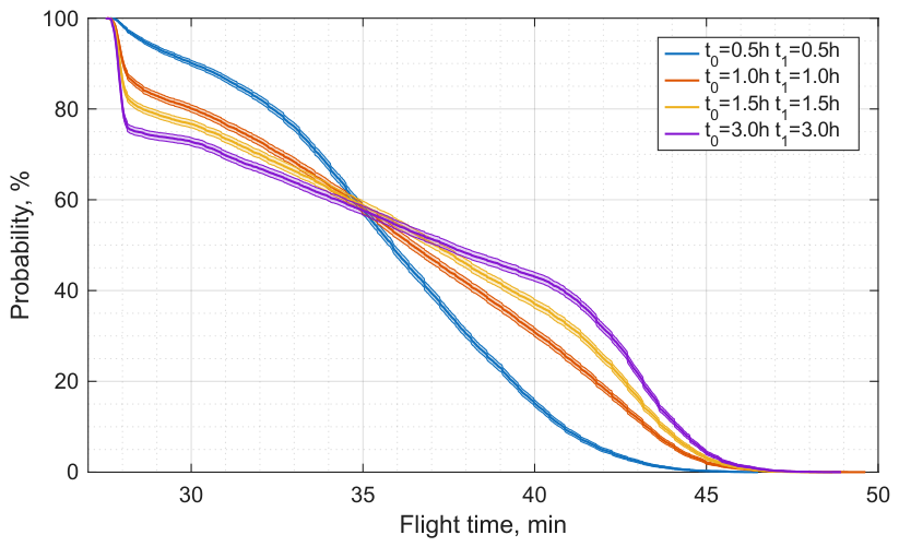
To analyse the impact of state persistence and transition frequencies on flight duration, perfectly symmetric conditions ($t_0=t_1$) were investigated and are illustrated in Figure 11.

Across all symmetric scenarios, a flight of 35 min can be achieved with approximately 60% probability. This intersection point also marks a complete trend reversal in operational risk: for shorter target flight times, longer mean state durations result in a reduced probability of mission success, whereas the opposite holds true for the extended flight durations.

This behaviour is driven by the statistical variance of the weather transitions relative to the total mission time, as when state durations are short ($t_0=t_1=0.5$ h), the rapid, frequent switching between clear-sky and cloud cover averages out the net power. When the state durations scale upward ($t_0=t_1\ge 1.0$ h) this effect is lost as the UAV is either under prolonged cloudy conditions that deplete the battery, or in an extended clear-sky state that maximises energy harvesting. This is also reflected in the survival probability, which for the short-lasting mean states ($t_0=t_1=0.5$ h) is initially concave and becomes convex after the inflection point, while the opposite pattern is observed when the mean states duration increase.

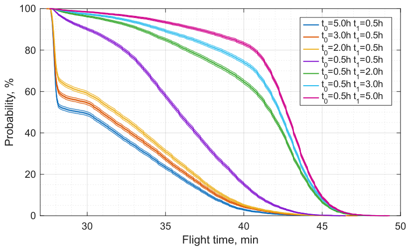
Limits of the cloud-cover influence were captured under extreme meteorological scenarios presented in Figure 12, which include the highly variable symmetric case alongside severe state imbalances.

When a heavily cloud-dominated environment is investigated ($t_0\in \{3.0,5.0\},t_1=0.5$ h), the survival probability drops immediately after reaching the abovementioned 28 min threshold to a 50–60% level, reflecting a high probability of encountering a dominant, long-duration cloud layer early in flight. Conversely, when an extreme sun-dominated environment is evaluated ($t_0=0.5,t_1=\in \{3.0,5.0\}$ h), the exact opposite effect is observed: the survival probability gradually decreases up to approximately 40 min and then rapidly drops. This steep decline represents the impact of a reduction in solar irradiance and UAV design constraints, mainly the solar array area and battery size. These combined findings prove that under the Central European regime, cloud cover can noticeably reduce flight time even during theoretically optimal summer periods and must be accounted for.

7.3. Cloud Cover Type

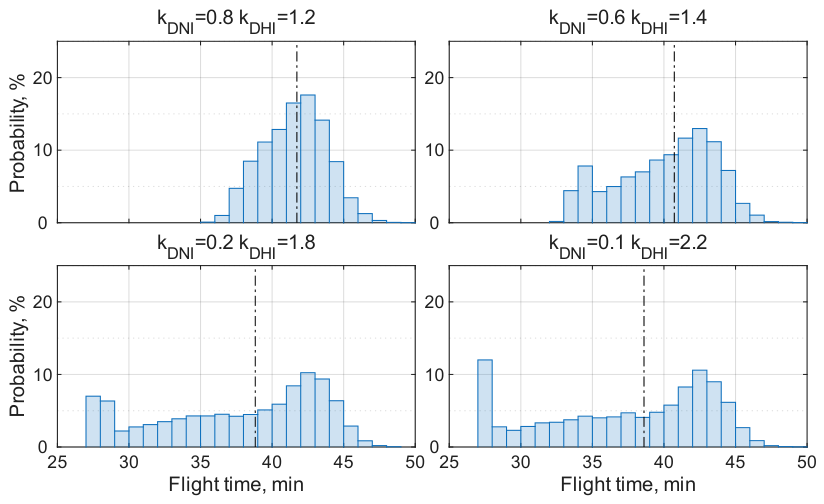
The influence of cloud cover type on flight duration was evaluated for four atmospheric scenarios (near-clear sky, light clouds, moderate clouds and heavy overcast) under stable atmospheric conditions ($t_0=1.0$ h, $t_1=1.5$ h) on 15 July at 12:00 LST. A Monte Carlo analysis comprising 10,000 simulations was conducted, and the resulting flight-time probability distributions, discretised into 1 min intervals, are presented in Figure 13.

Under near-clear sky conditions ($k_{DNI}=0.8,k_{DHI}=1.2$), the flight-time distribution remains strongly concentrated around the median value of 41.7 min, with an asymmetric reduction, more pronounced for longer flight times. The introduction of light cloud cover ($k_{DNI}=0.6,k_{DHI}=1.4$) causes both a broadening and leftward shift of the distribution, reducing the median flight time to 40.7 min. At the same time, a secondary local probability peak appears within the 34–35 min interval, indicating an elevated risk of terminating the flight within this window.

With moderate cloud cover ($k_{DNI}=0.2,k_{DHI}=1.8$), the redistribution toward shorter flight durations becomes more pronounced. The median decreases further to 38.8 min, while the lower tail extends towards the 27–28 min range, where a distinct local maximum of 7.0% is observed. Under heavy overcast ($k_{DNI}=0.1,k_{DHI}=2.2$), this mechanism intensifies further, with probability from neighbouring short-duration intervals shifting into the 27–28 min bin. Consequently, this segment becomes the dominant mission outcome, reaching a peak probability of 12.0%. Despite the substantial degradation in atmospheric conditions, the median flight time decreases only slightly to 38.6 min.

These findings confirm the previous conclusions regarding the necessity of cloud modelling for solar-assisted UAV flight endurance under Central European conditions, as the operational risk profile varies with cloud cover type. Therefore, evaluating the probability of achieving a target flight duration must rely on meteorological forecasts that account for specific cloud characteristics.

7.4. Solar Area and Battery Capacity

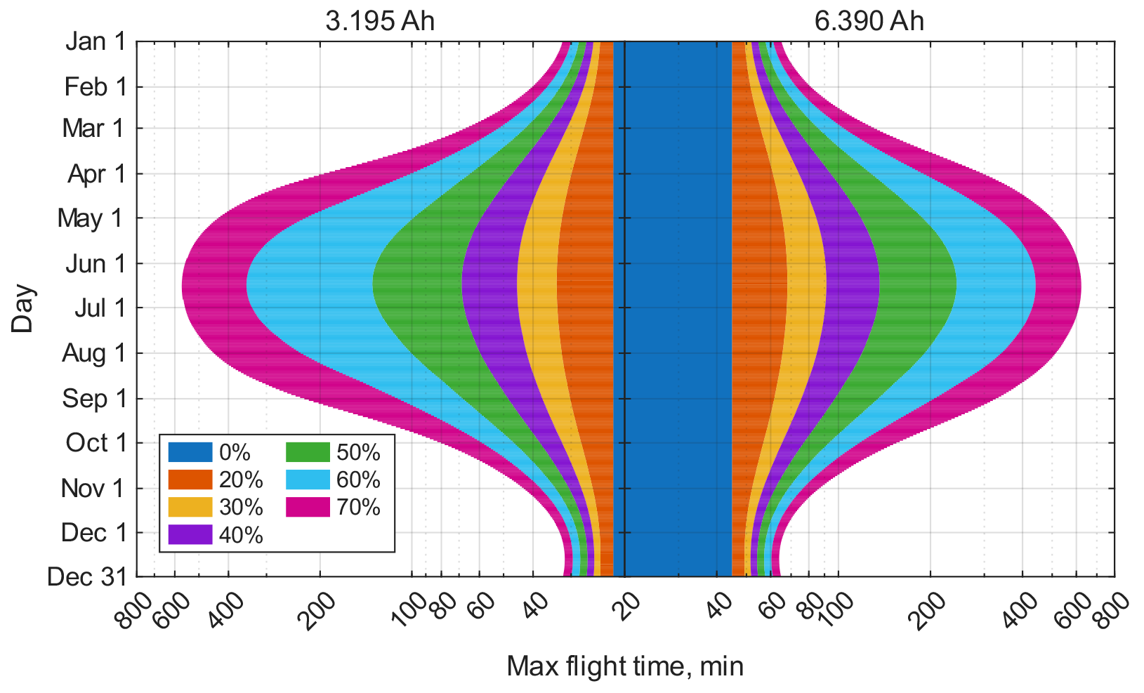
To evaluate the key design parameters’ impact on the solar-assisted UAV flight endurance, a comprehensive sensitivity analysis was conducted for the baseline and doubled battery capacity. The maximum achievable flight times throughout the year under clear-sky conditions are illustrated in Figure 14.

The analysis reveals that the flight time extension is most pronounced during the solar-energy-dominant part of the year and varies nonlinearly with increasing solar array area. For the default battery capacity of 3.195 Ah, the most significant performance shift is observed when increasing the solar area from 50% to 60% wing area coverage, which yields an endurance extension of up to 214 min. An additional 10% of solar coverage provides a further gain of up to 220 min, allowing the absolute maximum flight time to top at 569 min during the summer peak. A similar trend is observed when the battery capacity is doubled to 6.390 Ah. Notably, the underlying nonlinearity is even stronger as expanding the solar area from 50% to 60% provides an endurance gain of 198 min, whereas a subsequent 10% increase in solar coverage yields a diminishing value of 181 min, with the peak flight time topping at 622 min.

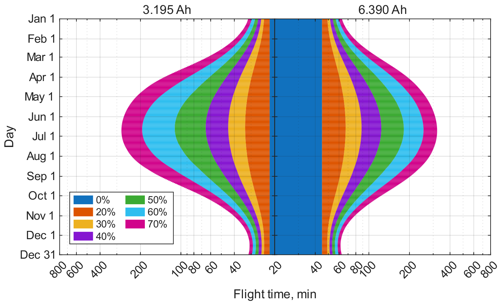
While these endurance peaks represent the system’s full capability when the entry time is actively optimised, practical mission planning often faces rigid operational constraints, including strict launch-time allocation. Consequently, operators may not always have the flexibility to deploy the UAV at the optimal time. To demonstrate the impact of such operational constraints, the flight endurance under median clear-sky irradiance, assuming a fixed mission start at solar noon, is presented in Figure 15.

This comparison highlights the UAV’s energy balance sensitivity to the mission scheduling. Restricting the mission start to solar noon reduces the total energy-harvesting potential compared to time-optimised scenarios. Specifically, the maximum achievable flight times are halved to 277 min for the standard battery and 321 min for the doubled-capacity variant. Despite this reduction, the results demonstrate that substantial solar-assisted endurance gains remain achievable even under such non-optimal scheduling. For the standard battery configuration, expanding the solar array from 50% to 60% and then from 60% to 70% of wing area coverage yields a maximum flight-time extension of 83 min in both cases. With the doubled battery capacity, this provides 72 and 67 min of gain, respectively. Overall, these scaling trends closely align with the optimised mission start analysis outcomes.

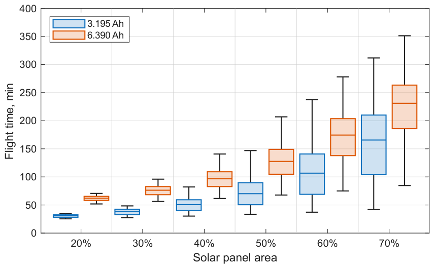
These findings demonstrate that low-altitude long-endurance aircraft operating under Central European conditions can successfully provide the required mission times when operations are performed under favourable clear-sky weather windows. However, for routine operations performed according to a given schedule, rather than isolated endurance-maximisation flights, the analysis must include stochastic cloud cover modelling as demonstrated earlier. The corresponding cloudiness impact for a realistic atmosphere under moderate cloudy conditions on 15 July, start at 12:00 LST, is shown in Figure 16.

When stochastic cloud cover is incorporated into the simulation, the nonlinear relationship between the flight endurance and the solar array wing coverage remains preserved for the median values across both battery capacities. Specifically, at the maximum investigated solar coverage of 70%, the median flight times reach approximately 166 and 231 min for the default and doubled battery capacities, respectively. This represents a substantial degradation compared to the clear-sky limits of approximately 262 and 308 min observed for 15 July (solar noon start) and further underscores the necessity of stochastic cloud cover modelling for realistic performance evaluation under the Central European climate.

Furthermore, the statistical dispersion of the results reveals critical insights into the operational risk profile. The middle 50% of the flight time distribution expands nonlinearly as the solar area increases, exhibiting a growing downward skewness. This asymmetry becomes even more prominent when examining the minimum and maximum values (excluding outliers). The physical mechanism driving this behaviour is directly linked to heavy overcast scenarios, as a dense and persistent cloud layer effectively nullifies the structural gains of increased solar area size. Consequently, the lower endurance limit demonstrates that expanding the solar collection area increases the operational upside but fails to guarantee a higher flight time floor during adverse weather conditions.

Although this study focuses on a fixed diamond-shaped pattern chosen to match the strict altitude-stability constraints of monitoring missions, two alternative profiles were also investigated. These included a standard search-and-rescue lawn-mower grid and a variable-altitude diamond path, where the UAV alternates between completing a full diamond at the baseline altitude, climbing by 25 m during a 400 m straight rectilinear transition segment (preceded and followed by a 50 m buffer after and before turns), and then completing the subsequent diamond at the new ceiling before returning to the baseline altitude and completing the new diamond. The comparative tests showed that the observed energy-related boundaries and non-linear degradation trends remained remarkably uniform across all profiles if the mean power consumption over the repetitive part was equivalent.

7.5. Battery and PV System Uncertainty

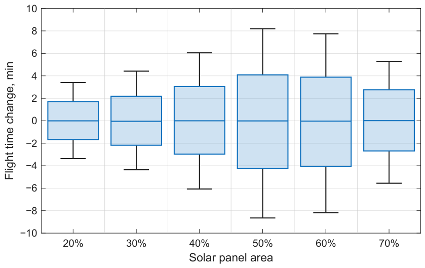
To evaluate the battery system’s uncertainty impact on the solar-assisted UAV flight time, a comprehensive sensitivity analysis was conducted for the default configuration under median-adjusted irradiance and clear-sky conditions, varying the battery parameters by ±10% across 10,000 Monte Carlo runs. The corresponding change in flight time across the varying solar area coverage for the default battery settings, evaluated for 15 July (start at 12:00 LST), is shown in Figure 17.

The results demonstrate a low asymmetry in interquartile ranges and extreme values across all investigated solar-to-wing area ratios. For 20–50% solar coverage, a progressive broadening of the operational uncertainty is observed, with the IQR maximum deviation reaching approximately ±4 min and the min–max values extending up to approximately twice that range. This trend reflects a regime in which the limited solar area forces the UAV to rely more on its stored reserves, making the overall flight time and mission success probability more sensitive to deviations in internal battery characteristics.

A trend reversal occurs near 60% solar coverage, and the dispersion starts to contract as the PV system provides a sufficient operational margin, consistently bringing the battery to its maximum state of charge. Any minor change in the battery’s electrochemical parameters is effectively buffered by the excess solar energy, thereby masking the variations in cell performance. Thus, the battery system exhibits localised robustness for a given mission schedule when the solar-harvesting array is optimally sized.

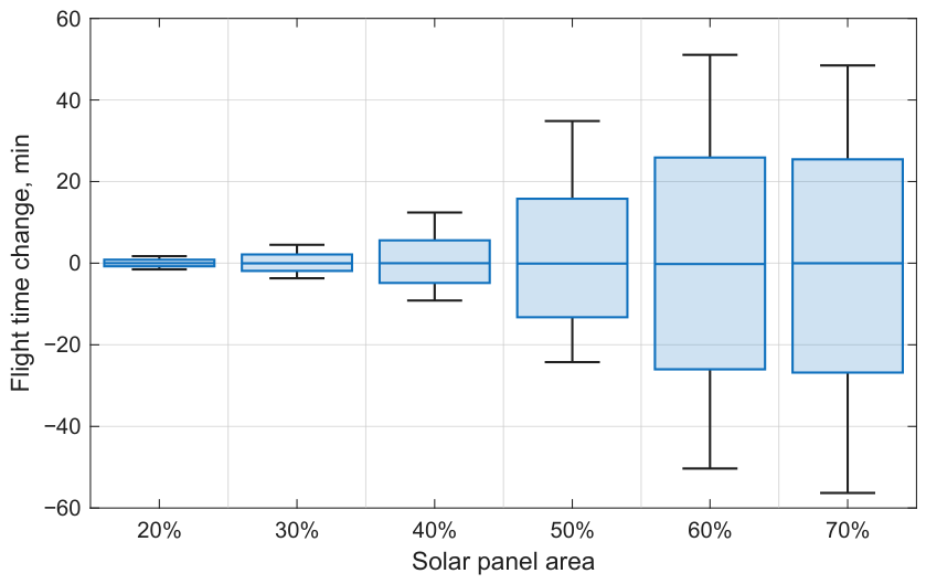
The same analysis type was performed to assess the influence of solar panel efficiency on the solar-assisted UAV flight time, with the only difference that, instead of varying the battery parameters by ±10%, the analysis was performed relative to the cell reference efficiency ${\eta }_{c,ref}$. The corresponding change in flight time across the varying solar area coverage scenarios, evaluated for 15 July (start at 12:00 LST), is shown in Figure 18.

In contrast to the battery-induced variations, the PV efficiency uncertainty introduces significantly larger dispersions in flight time, with the interquartile range expanding from approximately 1.6 min at 20% coverage to 52 min at the large solar areas. Operational uncertainty increases within the 20–60% coverage range, reflecting the PV system’s power generation capability. Starting at 60% coverage, the uncertainty bounds begin to stabilise, which is driven by a battery saturation effect; under optimal or excessive solar area sizing, the baseline flight time is extended into later hours of the day when less solar radiation is available, and the irradiance falls below the level required to offset battery depletion.

This phenomenon is clearly reflected in the maximum values, where the variation in the upper extreme drops from 51.07 to 48.47 min for the 60% and 70% scenarios, respectively. When mapped to the total values, these variations correspond to absolute flight times of 231.18 and 310.90 min, demonstrating that the rigid ceiling imposed by the fixed battery capacity effectively clamps further variance as the day progresses. This physical limitation also induces a downward asymmetry in the extreme values, with the minimum values dropping by 50.32 and 56.31 min relative to the corresponding absolute flight time.

Consequently, this demonstrates the existence of an engineering optimum: expanding the PV area stabilises nominal performance but shifts the mission end to late-day hours, where any efficiency loss can penalise flight duration.

7.6. High Solar Coverage Scenario

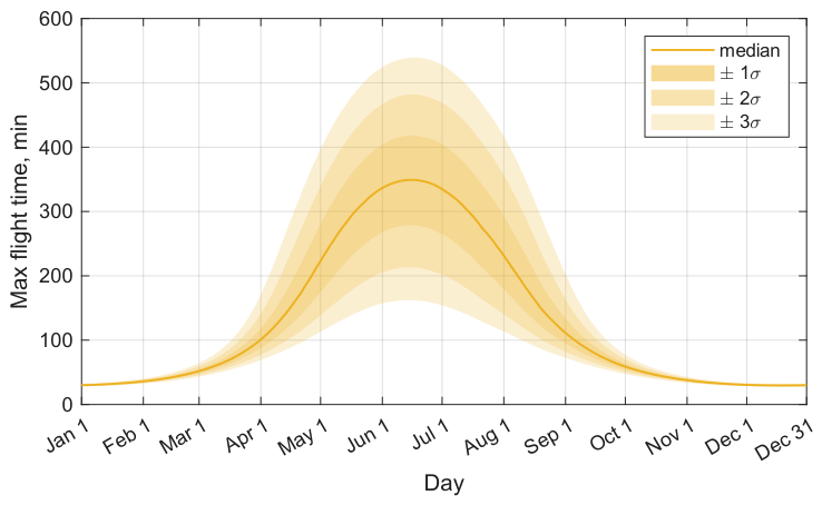
To verify the behavioural consistency and scalability under enhanced design parameters, the low-altitude long-endurance UAV with 60% wing area coverage was investigated, as this scenario yielded the largest flight time gains. The maximum clear-sky flight time throughout the year, along with its associated variability limits, is illustrated in Figure 19.

The resulting flight time profile reflects the core structural characteristics obtained for the default configuration but scales toward longer flight times. The minimum clear-sky flight time increases to 30 min, extending the battery-only baseline by 8 min. If the 10% performance impact threshold discussed in the baseline clear-sky analysis is applied, the energy-efficient operational band expands substantially, beginning in mid-February and extending through late October. However, it must be emphasised that during the winter-to-spring and autumn-to-winter transitions, frequent frontal passages and atmospheric transitions induce elevated cloudiness levels in Central Europe, which as previously shown, must be accounted for. Moreover, the short day-length during these periods reduces the daily operational window, thereby increasing the risk that a specific day will completely lack a time segment with adequate irradiance levels.

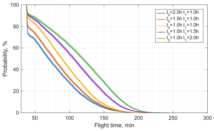
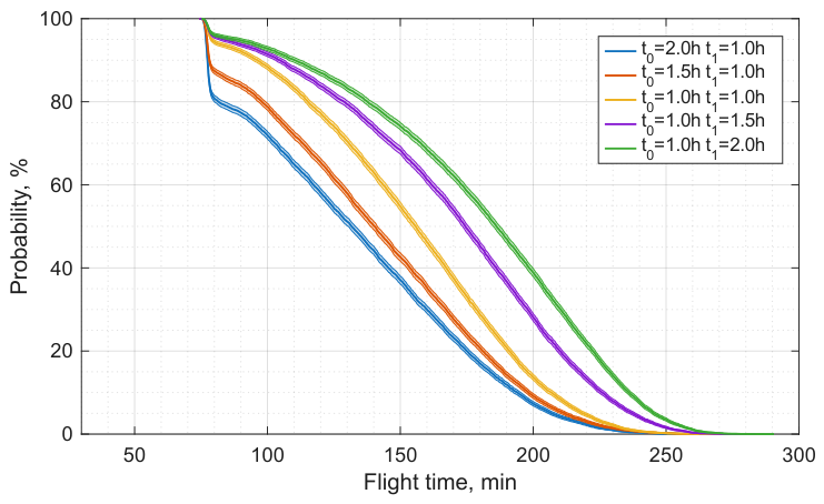
To establish a direct comparison with the default design, the mission survival probability on 15 July, starting at 12:00 LST, under a realistic atmosphere with moderate cloud cover was evaluated for both the default battery capacity and the doubled capacity variant. These stochastic evaluations are presented in Figure 20 and Figure 21, respectively.

The survival probability structural characteristics for the default battery capacity closely follow the trends observed for the baseline scenario. The minimum flight time increases to 37 min, and the inflection point is marginally shifted beyond this threshold, reaffirming the persistent limiting influence of heavy overcast conditions regardless of the increased solar array size. When cloud-dominated weather states strongly prevail, a 50% survival probability is achieved at 70 min, which extends to 120 min under sun-dominated conditions. This represents an approximate two- and three-fold increase compared to the baseline configuration, confirming that increasing the solar area serves as an effective risk mitigation strategy against atmospheric variability.

For the doubled battery capacity, the minimum flight time rises to 75 min, nearly doubling the standalone battery-only limit. This design also mitigates the heavy overcast penalties: the expanded energy storage provides the necessary operational margin to survive prolonged cloud states and transition into more favourable solar-harvesting conditions. However, the operational risk is not entirely eliminated. Flight durations of 132 and 186 min are achieved with a 50% probability for cloud- and sun-dominated regimes, respectively. Notably, the 132 min flight time under cloud-moderated conditions surpasses the 120 min observed under the sun-dominated regime for the default battery configuration. This facilitates the evaluation of the influence of battery capacity on weather resilience through harvested solar-energy buffering.

8. Conclusions

This paper presented a comprehensive stochastic simulation framework for assessing the operational feasibility of small-scale, low-altitude, solar-assisted UAVs under Central European meteorological conditions. It incorporates a locally adjusted ASHRAE irradiance model coupled with a semi-Markov process to describe cloud-to-sun transitions and cloud cover types. These environmental inputs are integrated with full rigid-body flight dynamics, a cascaded autopilot and the battery evaluation subsystem, so the framework successfully shifts from idealised clear-sky evaluation to a realistic, probabilistic representation of atmospheric attenuation effects on the flight time.

The study demonstrated that the conventional deterministic clear-sky parameterisation substantially overestimates the energy harvesting potential of low-altitude solar-assisted UAVs. Relying on such idealised models creates an overly optimistic operational outlook, which could precipitate unexpected power exhaustion and catastrophic mission failure in practical field deployments.

It was found that under clear-sky conditions, the solar panels exert a highly nonlinear influence on maximum flight times, establishing a theoretical flight time ceiling for a low-altitude long endurance UAV of approximately 569 and 622 min on June 15 when the mission start time is optimised, initial battery SOC is at 70%, and no additional power losses (e.g., due to crosswind) are considered. Maximising this endurance necessitates precise mission timing as initiating flights early in the morning (at 07:00 and 06:30, respectively) allows the platform to achieve battery state-of-charge saturation prior to solar noon. This strategy optimises energy storage retention during peak irradiance, effectively buffering the system before transitioning to a gradual, unassisted battery discharge as solar input diminishes. When the mission starts at solar noon, under the same constraints, the flight times are reduced to 277 and 321 min, respectively.

Atmospheric variability introduces significant operational constraints. Under moderate cloud cover conditions with missions initiated at solar noon, the median endurance decreases markedly. This indicates the necessity for optimising launch time for endurance-maximising flights as well as cloud cover modelling requirements for routine operations performed according to a fixed schedule.

Additionally, a severe atmospheric constraint exists under heavy overcast conditions, marked by a sharp and significant drop in the mission survival probability function. Crucially, this threshold limitation persists regardless of the wing solar coverage ratio, leading to a profound operational asymmetry: while an increased PV area expands the upper bound of operational gains under favourable conditions, it fails to elevate the minimum guaranteed flight endurance. Under heavy overcast scenarios, direct and diffuse atmospheric irradiance yields a power input that slightly prolongs flight time compared to a battery-only baseline. To meaningfully mitigate, rather than completely eliminate, the operational risks associated with heavy overcast, emphasis must shift from expanding photovoltaic harvesting surfaces to enhancing energy storage capacity, as scaling the battery system enables the aircraft to sustain operations through transient periods of high atmospheric attenuation while awaiting improved irradiance conditions.

Future research directions can focus on employing this framework to analyse alternative solar-powered UAV configurations operating under different climatic regimes. Furthermore, the developed stochastic simulation model can be integrated with real-time meteorological forecasts, serving as a data generation baseline for Artificial Neural Network training aimed at predictive mission planning and optimisation under operational requirements. Additionally, future extensions could incorporate adaptive flight-path optimisation algorithms, enabling the UAV to dynamically adjust its course to maximise solar irradiance and avoid localised cloud cover. Finally, the methodological approach established in this study exhibits high transferability and can be readily extended to adjacent engineering domains, including energy harvesting estimation for solar electric vehicles and supplementary power management in autonomous solar-powered robotics.