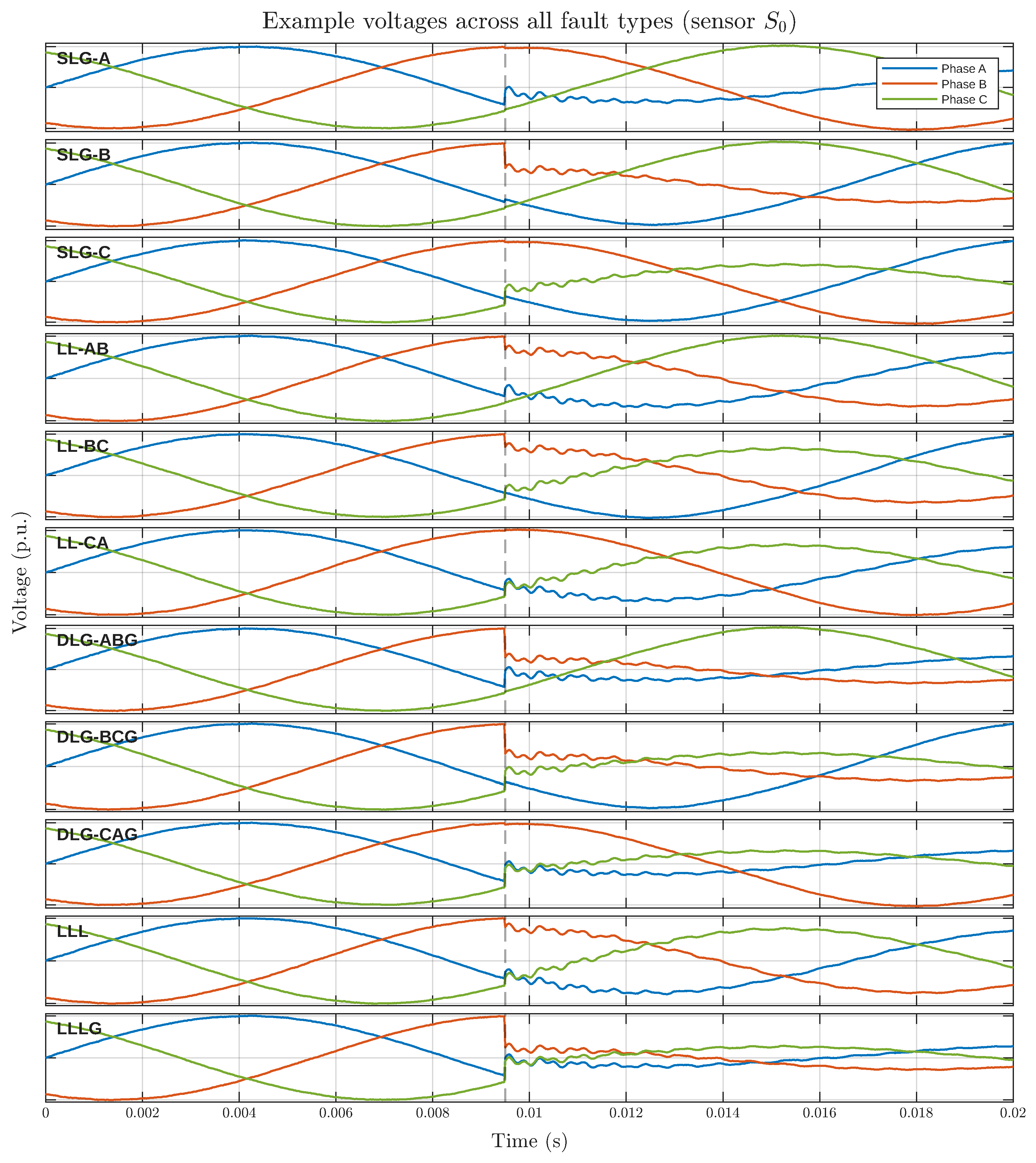
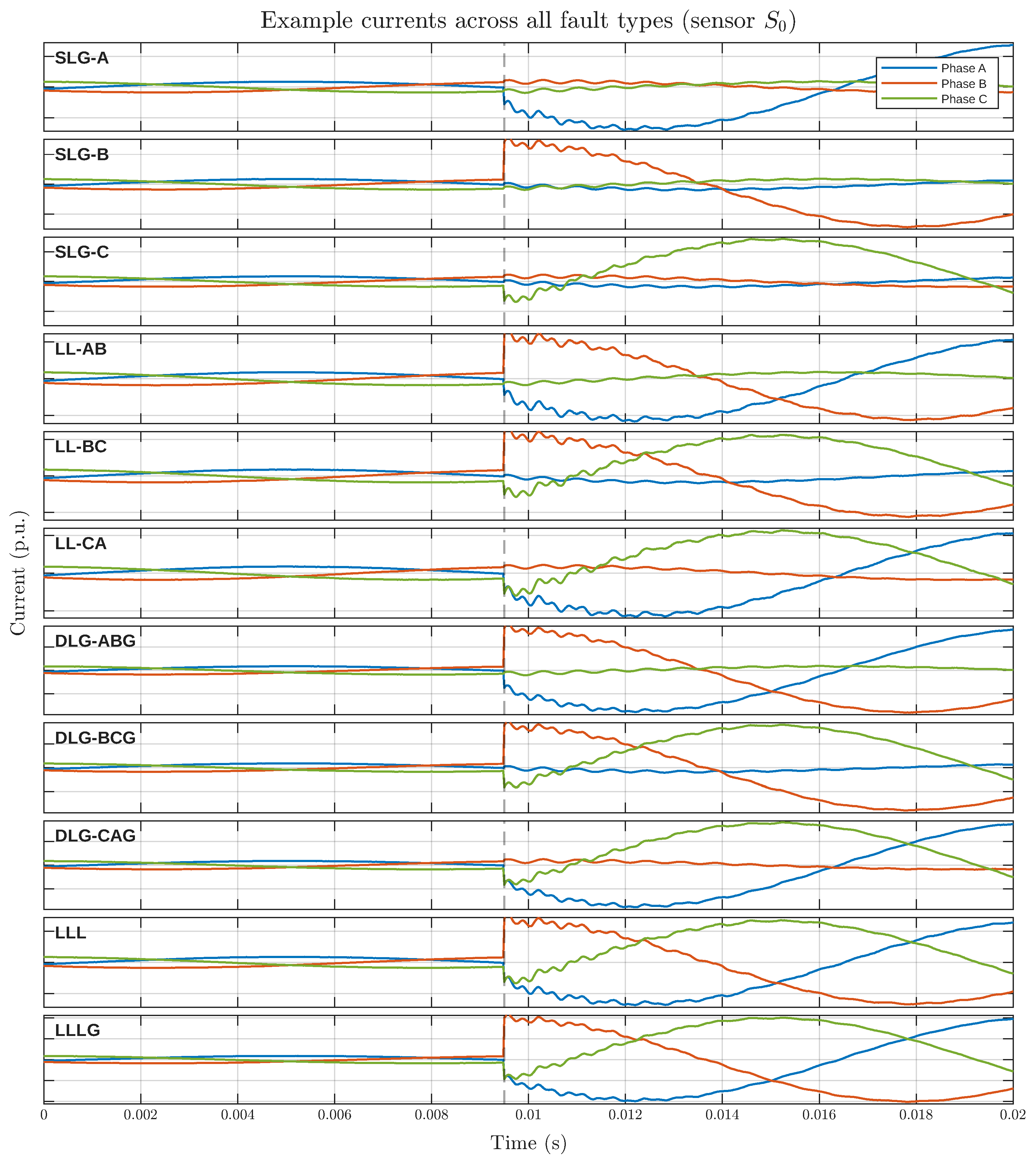
Figure 1.
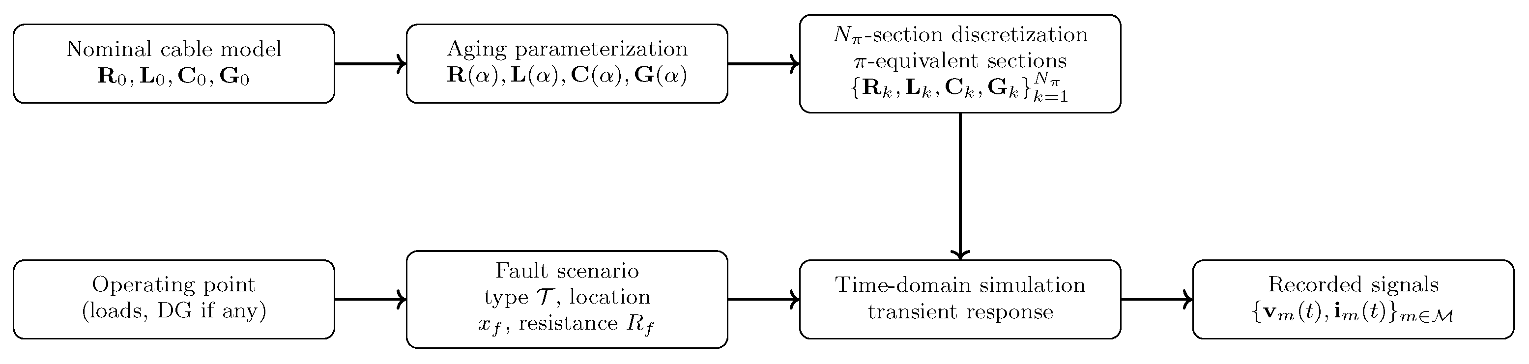
Aging-aware modeling workflow: nominal cable parameters are degraded via a normalized aging-stress index , discretized into cascaded -sections, and combined with operating conditions and an explicit fault scenario as inputs to the time-domain simulation, which produces transient voltage and current measurements.
Figure 1.
Aging-aware modeling workflow: nominal cable parameters are degraded via a normalized aging-stress index , discretized into cascaded -sections, and combined with operating conditions and an explicit fault scenario as inputs to the time-domain simulation, which produces transient voltage and current measurements.
Figure 2.
Electrical modeling hierarchy for underground cables: distributed parameters and telegrapher equations are approximated by cascaded -sections for time-domain transient simulation.
Figure 2.
Electrical modeling hierarchy for underground cables: distributed parameters and telegrapher equations are approximated by cascaded -sections for time-domain transient simulation.
Figure 3.
Aging parameterization: a normalized aging-stress index is mapped to aged per-unit-length cable matrices used by the electrical model.
Figure 3.
Aging parameterization: a normalized aging-stress index is mapped to aged per-unit-length cable matrices used by the electrical model.
Figure 4.
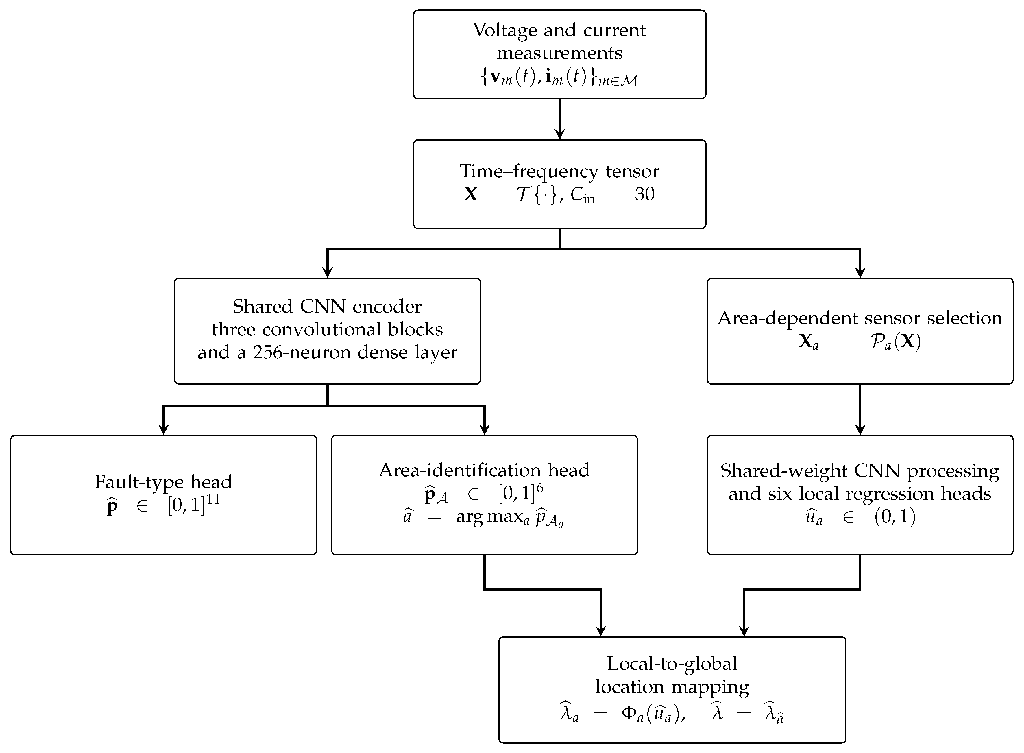
Unified architecture of the proposed Hybrid model. The complete time–frequency tensor is processed by the shared encoder for fault-type and feeder-area identification. In parallel, fixed area-dependent channel selectors retain the sensor subsets associated with each feeder area. The selected tensors are processed using shared-weight convolutional operations and six local regression heads. During inference, the predicted area selects the corresponding local estimate, which is subsequently transformed into the global normalized fault location.
Figure 4.
Unified architecture of the proposed Hybrid model. The complete time–frequency tensor is processed by the shared encoder for fault-type and feeder-area identification. In parallel, fixed area-dependent channel selectors retain the sensor subsets associated with each feeder area. The selected tensors are processed using shared-weight convolutional operations and six local regression heads. During inference, the predicted area selects the corresponding local estimate, which is subsequently transformed into the global normalized fault location.
Figure 5.
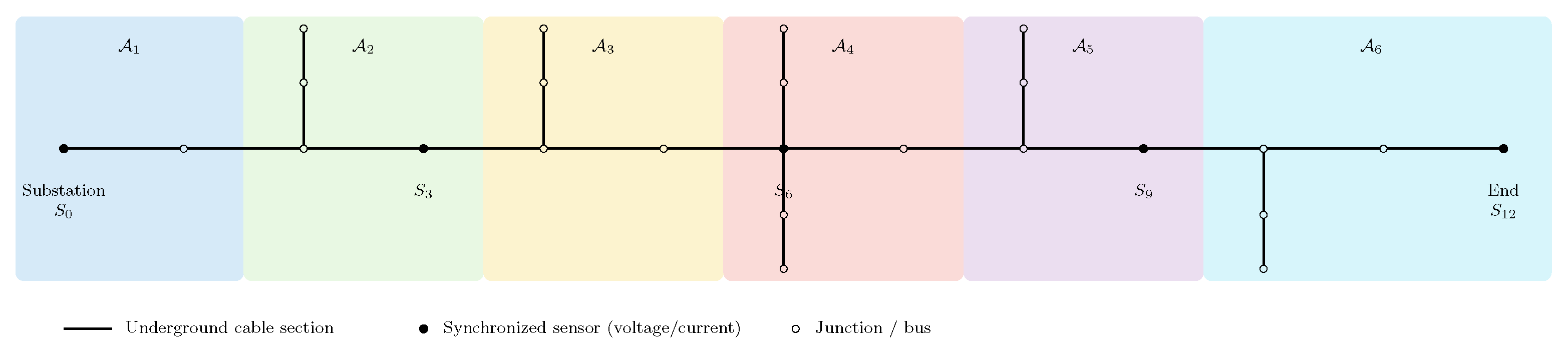
The large-scale underground feeder is partitioned into mutually exclusive and collectively exhaustive areas to enable area-wise coarse-to-fine fault localization in a branched network. Each lateral is assigned uniquely to the area of its root junction to avoid ambiguity in area labeling.
Figure 5.
The large-scale underground feeder is partitioned into mutually exclusive and collectively exhaustive areas to enable area-wise coarse-to-fine fault localization in a branched network. Each lateral is assigned uniquely to the area of its root junction to avoid ambiguity in area labeling.
Figure 6.
Coarse-to-fine area-wise localization strategy. The model first identifies the most probable feeder area and then estimates the in-area coordinate using the corresponding area-dependent sensor subset.
Figure 6.
Coarse-to-fine area-wise localization strategy. The model first identifies the most probable feeder area and then estimates the in-area coordinate using the corresponding area-dependent sensor subset.
Figure 7.
Large-case study workflow for aging-aware scenario generation, transient simulation, dataset labeling, and hybrid physics-regularized explainable inference.
Figure 7.
Large-case study workflow for aging-aware scenario generation, transient simulation, dataset labeling, and hybrid physics-regularized explainable inference.
Figure 8.
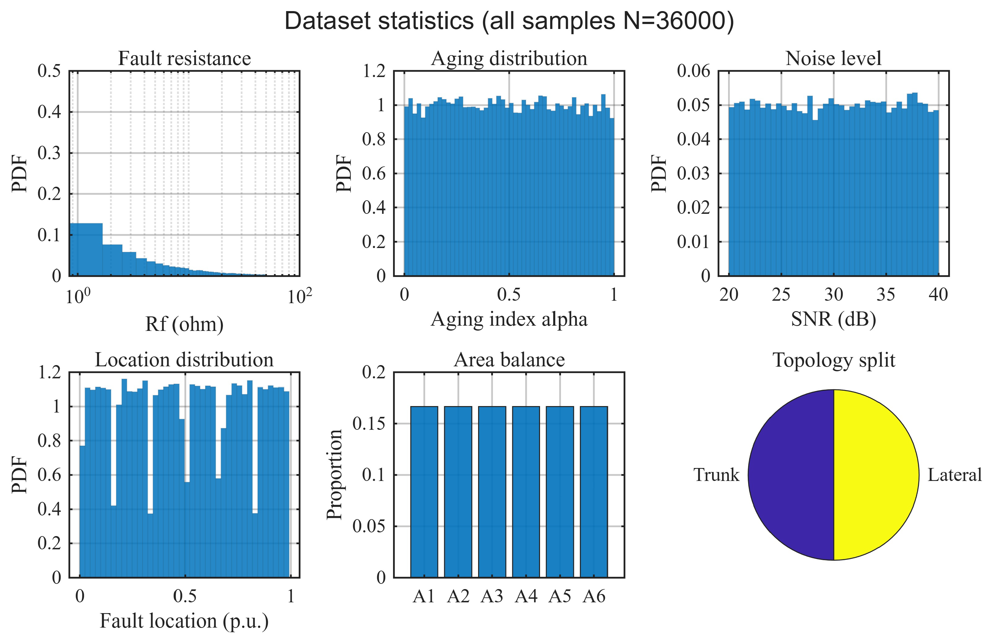
Dataset statistics for all generated samples: distributions of , normalized aging-stress index , SNR, fault location , area balance, and trunk/lateral topology split. These distributions verify broad coverage over the scenario variables and reduce the risk of biased aggregate metrics.
Figure 8.
Dataset statistics for all generated samples: distributions of , normalized aging-stress index , SNR, fault location , area balance, and trunk/lateral topology split. These distributions verify broad coverage over the scenario variables and reduce the risk of biased aggregate metrics.
Figure 9.
HF-envelope voltage waveforms across all fault types for a representative scenario at a fixed sensor. The row-wise layout highlights phase-dependent transient energy around fault inception, which is consistent with traveling-wave-based interpretation.
Figure 9.
HF-envelope voltage waveforms across all fault types for a representative scenario at a fixed sensor. The row-wise layout highlights phase-dependent transient energy around fault inception, which is consistent with traveling-wave-based interpretation.
Figure 10.
HF-envelope current waveforms across all fault types for the same scenario as
Figure 9. Current signals provide complementary transient information that enhances discrimination among fault categories and supports localization.
Figure 10.
HF-envelope current waveforms across all fault types for the same scenario as
Figure 9. Current signals provide complementary transient information that enhances discrimination among fault categories and supports localization.
Figure 11.
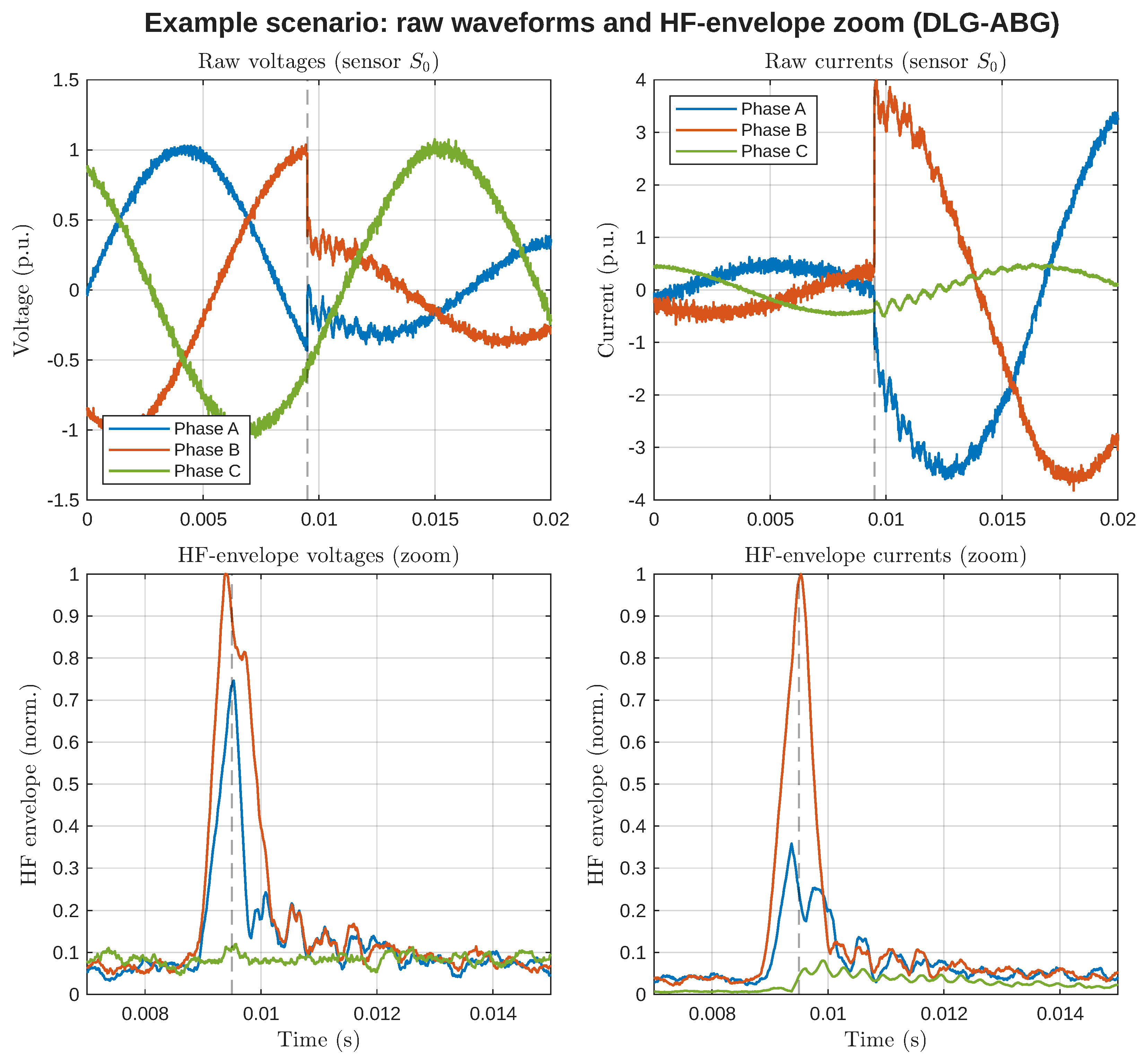
Comparison between raw three-phase signals and HF-envelope representations for an illustrative fault scenario. The envelope emphasizes transient energy and improves the visibility of fault inception and phase involvement. The dashed vertical line indicates the simulator-defined fault-inception instant.
Figure 11.
Comparison between raw three-phase signals and HF-envelope representations for an illustrative fault scenario. The envelope emphasizes transient energy and improves the visibility of fault inception and phase involvement. The dashed vertical line indicates the simulator-defined fault-inception instant.
Figure 12.
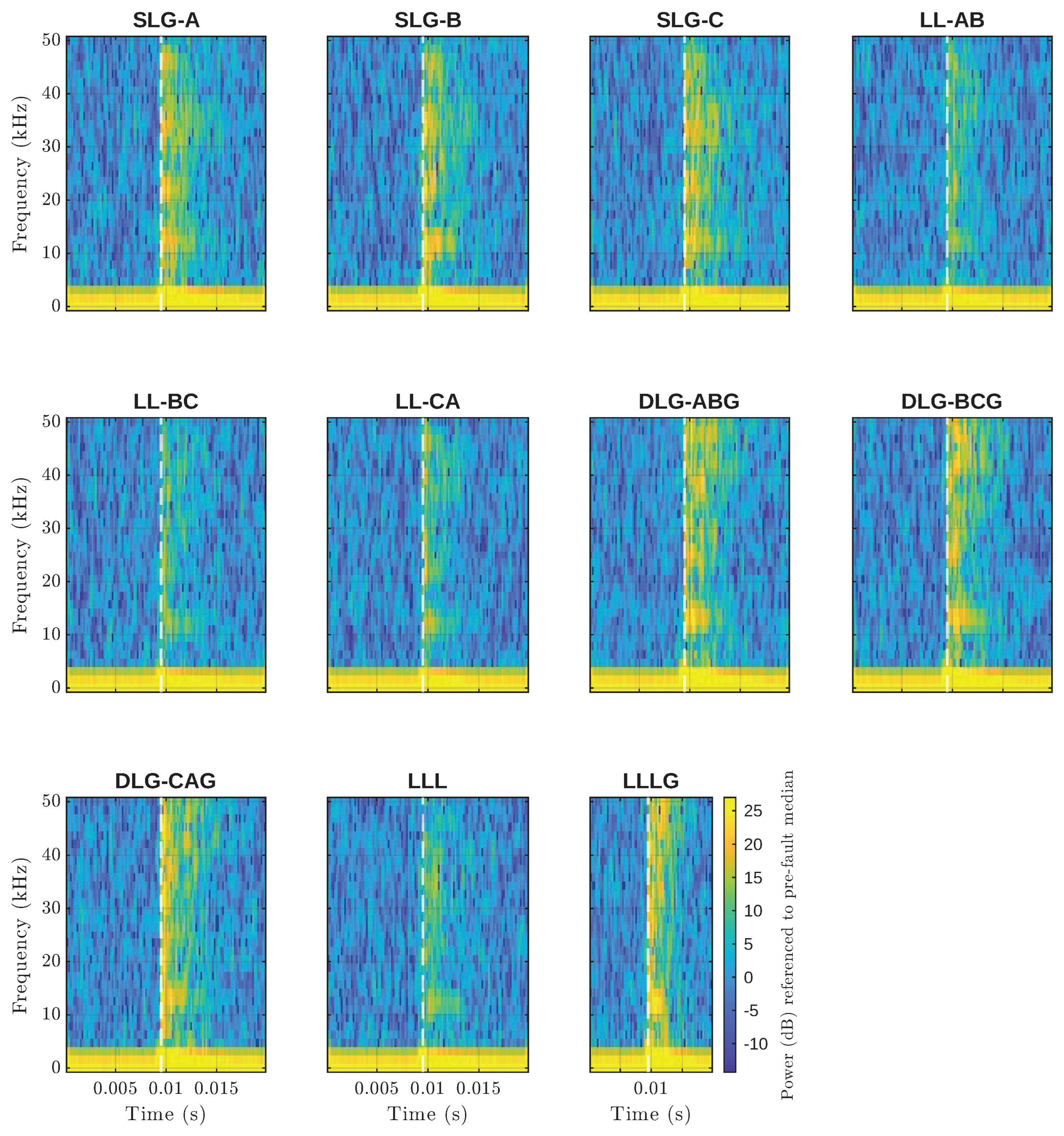
Time–frequency maps for all fault types using a high-frequency voltage residual at sensor . Each subplot shows a localized broadband energy increase around fault inception, indicated by the dashed line, confirming transient behavior consistent with traveling-wave propagation rather than stationary noise.
Figure 12.
Time–frequency maps for all fault types using a high-frequency voltage residual at sensor . Each subplot shows a localized broadband energy increase around fault inception, indicated by the dashed line, confirming transient behavior consistent with traveling-wave propagation rather than stationary noise.
Figure 13.
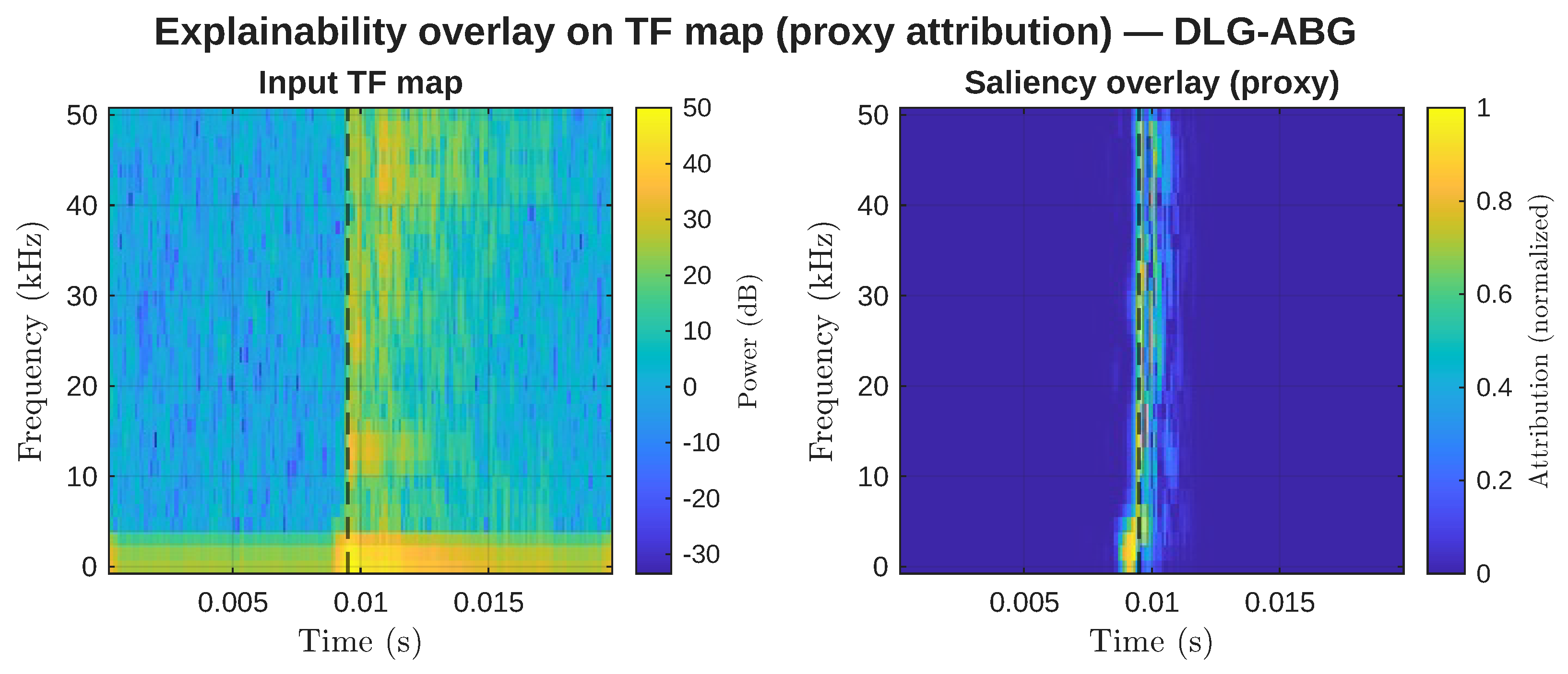
Qualitative time–frequency saliency illustration for a representative DLG-ABG fault at sensor . The left panel shows the input time–frequency representation, whereas the right panel shows a proxy saliency overlay constructed to emphasize the broadband transient region around the known simulated fault-inception instant. The proxy overlay is not a model-native Grad-CAM or SHAP attribution and is not used as quantitative evidence of explanation faithfulness.
Figure 13.
Qualitative time–frequency saliency illustration for a representative DLG-ABG fault at sensor . The left panel shows the input time–frequency representation, whereas the right panel shows a proxy saliency overlay constructed to emphasize the broadband transient region around the known simulated fault-inception instant. The proxy overlay is not a model-native Grad-CAM or SHAP attribution and is not used as quantitative evidence of explanation faithfulness.
Figure 14.
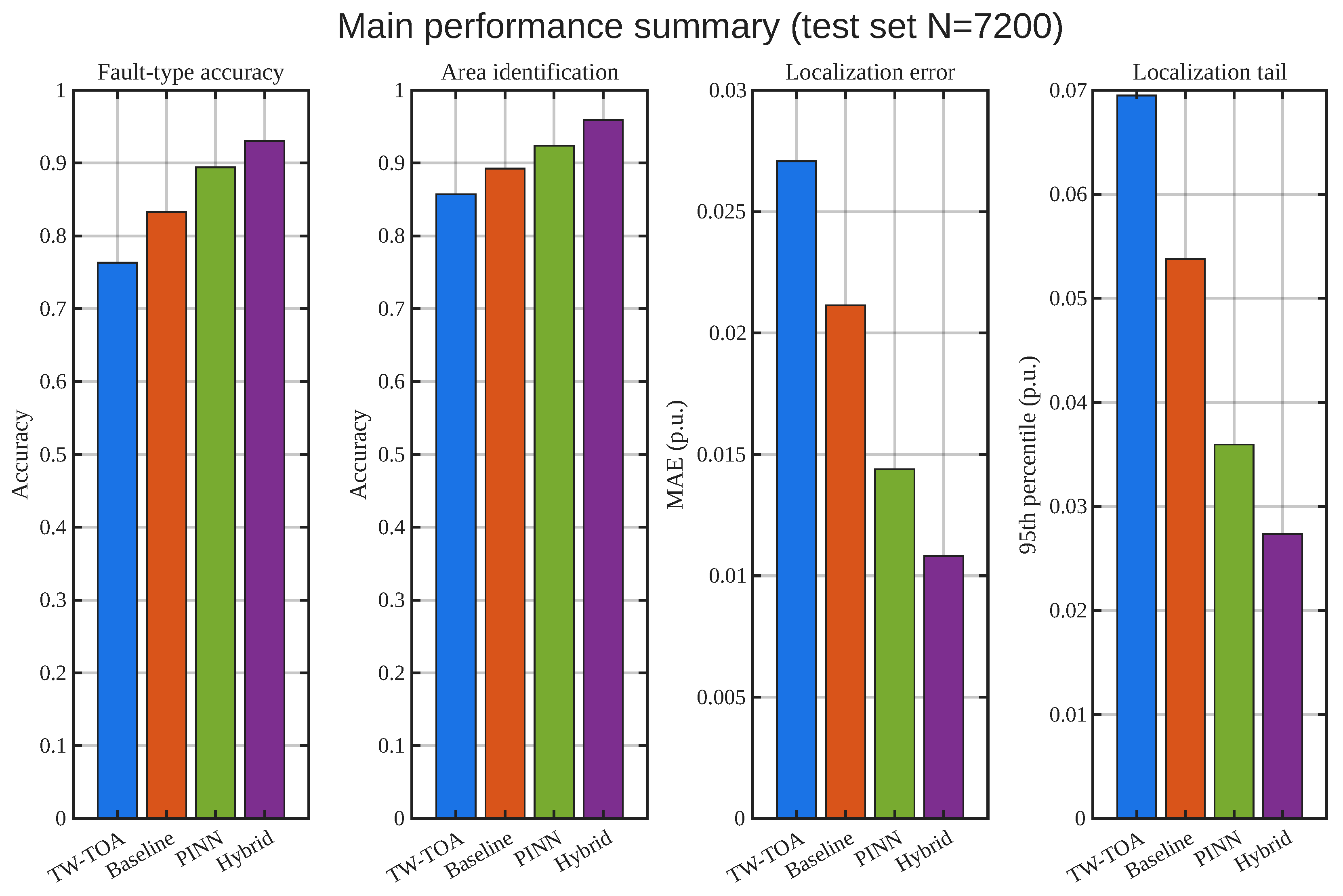
Main performance summary on the test set: fault-type accuracy, area-identification accuracy, localization MAE, and localization P95 across TW-TOA, Baseline, PINN, and Hybrid models. The Hybrid model consistently achieves the best performance across all metrics, including reduced tail error.
Figure 14.
Main performance summary on the test set: fault-type accuracy, area-identification accuracy, localization MAE, and localization P95 across TW-TOA, Baseline, PINN, and Hybrid models. The Hybrid model consistently achieves the best performance across all metrics, including reduced tail error.
Figure 15.
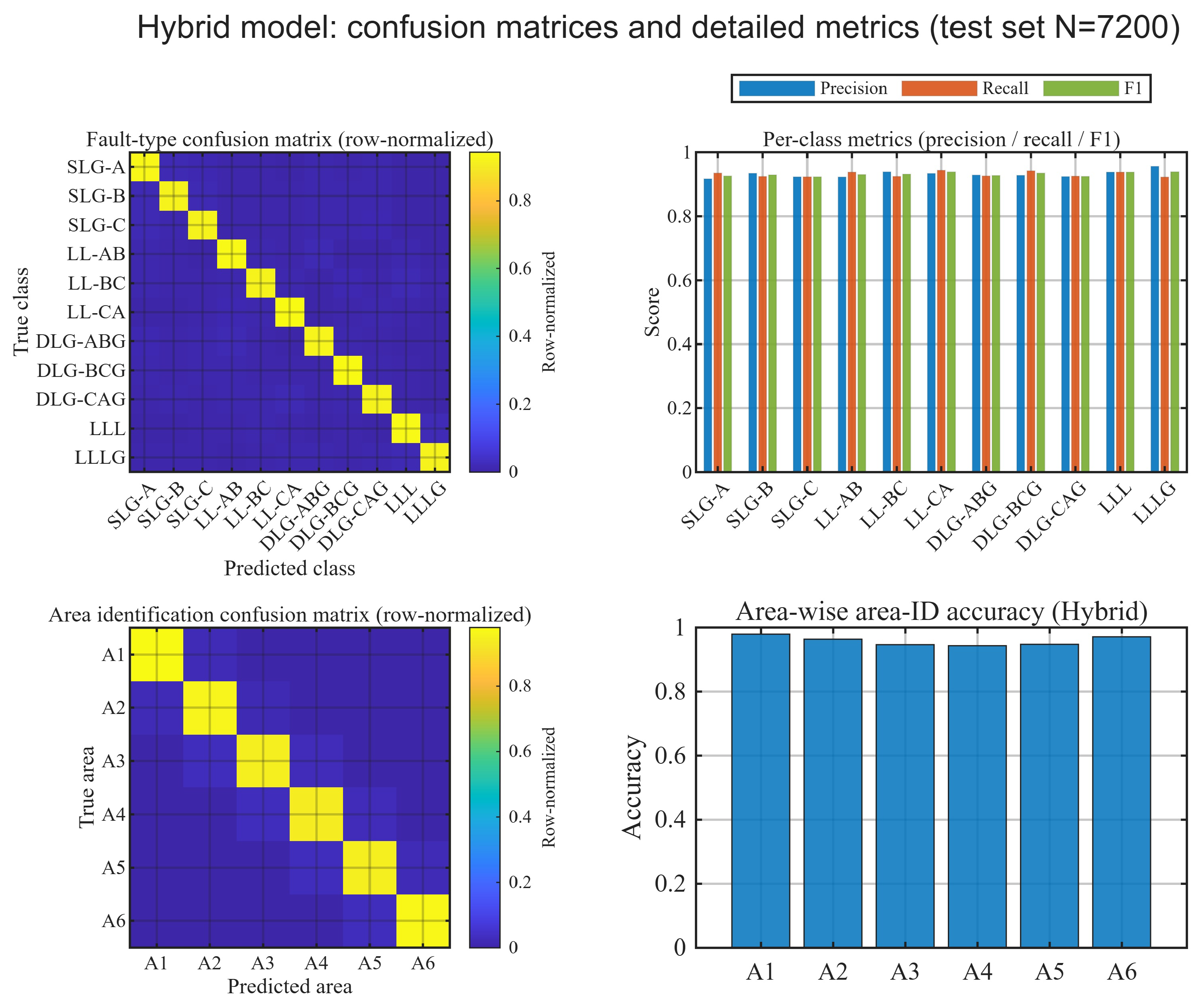
Hybrid diagnostic suite on the test set (): row-normalized fault-type confusion matrix with per-class precision, recall, and F1-score metrics, and row-normalized area-identification confusion matrix with area-wise accuracy. The dominant diagonal structure indicates accurate predictions, while the sparse off-diagonal entries are mainly associated with physically related fault types or neighboring feeder areas.
Figure 15.
Hybrid diagnostic suite on the test set (): row-normalized fault-type confusion matrix with per-class precision, recall, and F1-score metrics, and row-normalized area-identification confusion matrix with area-wise accuracy. The dominant diagonal structure indicates accurate predictions, while the sparse off-diagonal entries are mainly associated with physically related fault types or neighboring feeder areas.
Figure 16.
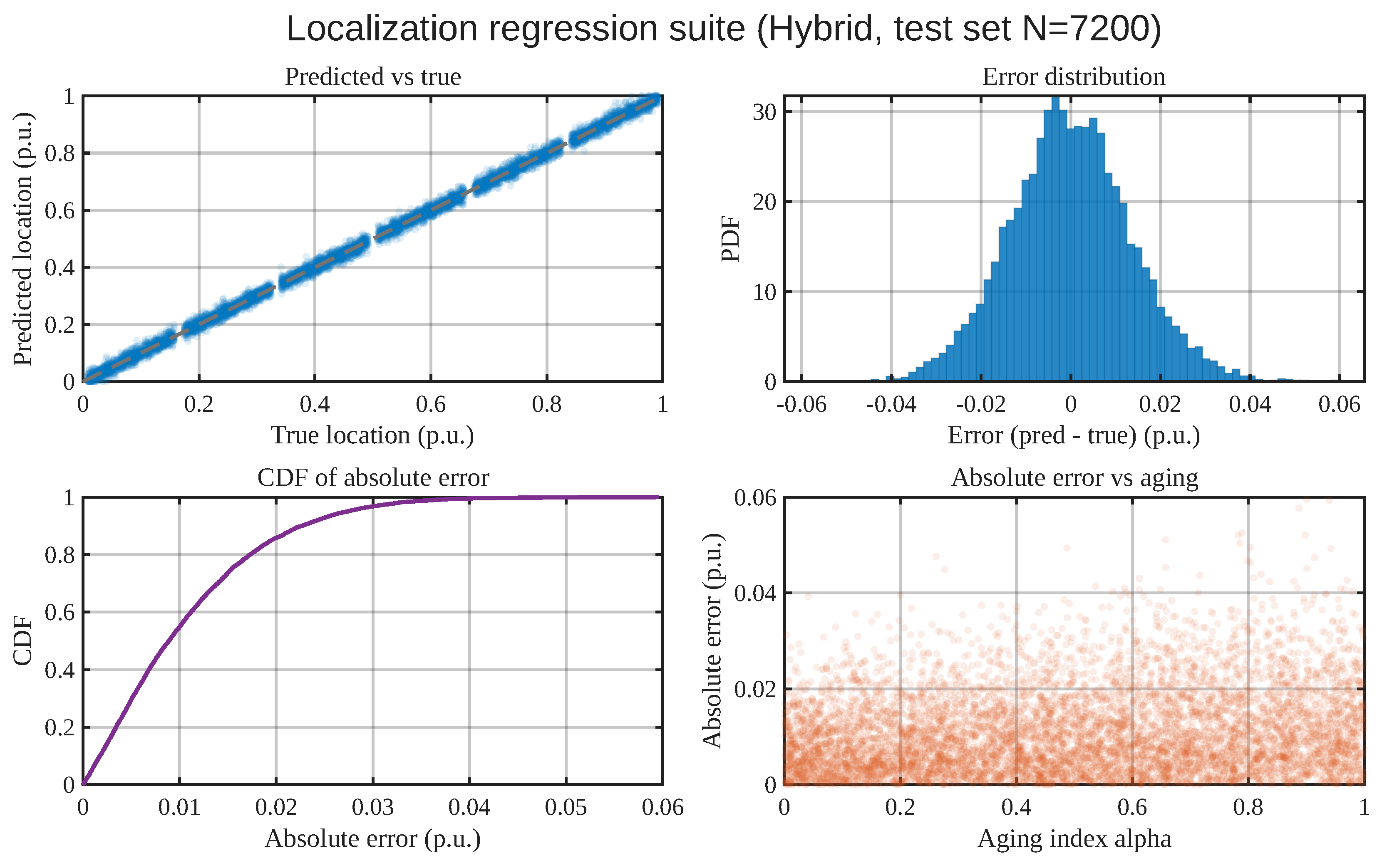
Hybrid localization regression diagnostics on the test set (): predicted versus true normalized location , signed error distribution, empirical CDF of absolute localization error, and absolute error versus normalized aging-stress index . These diagnostics evaluate bias, dispersion, tail behavior, and sensitivity to aging-induced parameter drift.
Figure 16.
Hybrid localization regression diagnostics on the test set (): predicted versus true normalized location , signed error distribution, empirical CDF of absolute localization error, and absolute error versus normalized aging-stress index . These diagnostics evaluate bias, dispersion, tail behavior, and sensitivity to aging-induced parameter drift.
Figure 17.
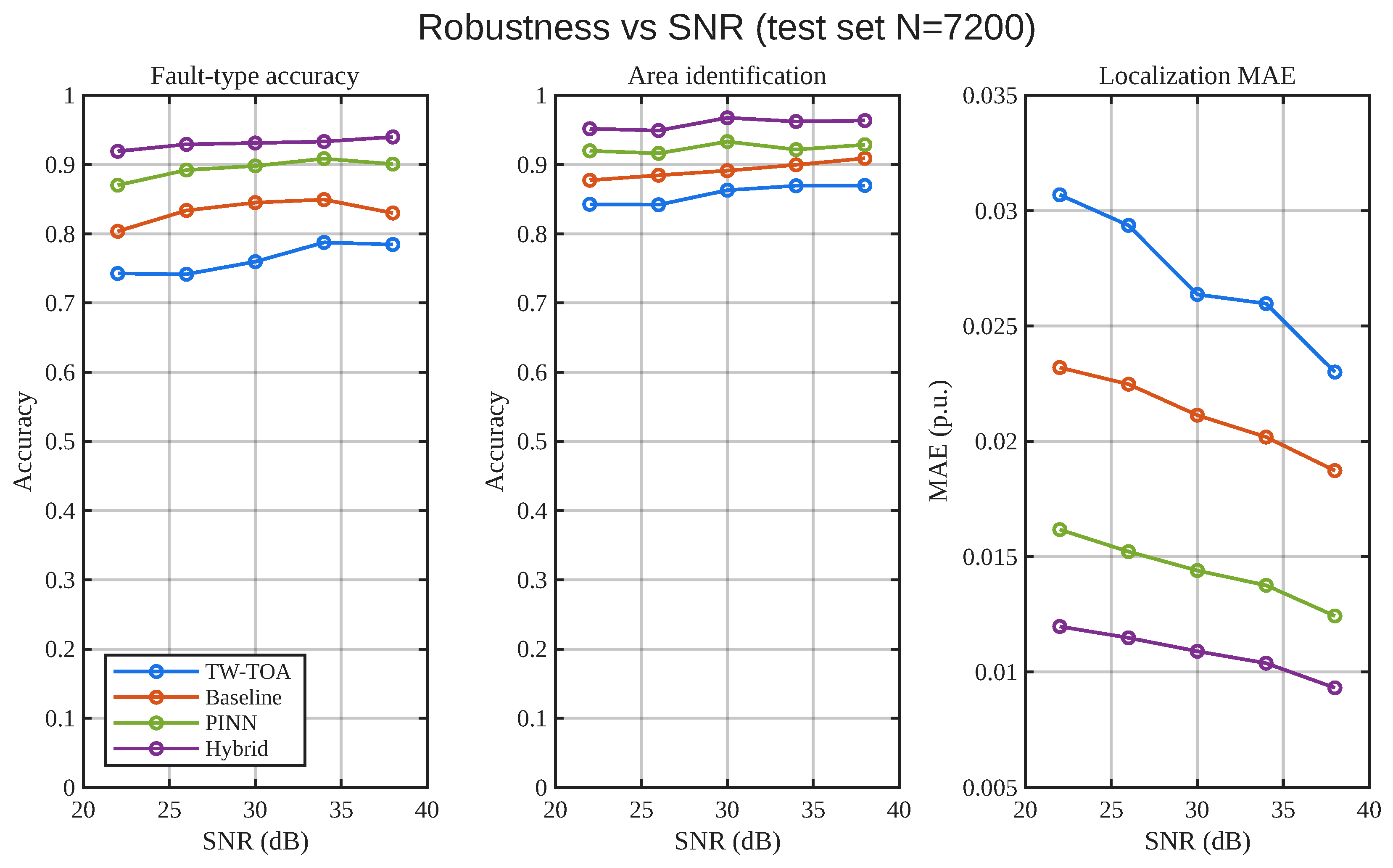
Binned test-set performance as a function of SNR over the simulated range of 20–: fault-type accuracy, area-identification accuracy, and localization MAE. Decreasing SNR degrades all configurations, while the Hybrid model retains the highest accuracies and the lowest MAE within the prescribed additive-noise domain.
Figure 17.
Binned test-set performance as a function of SNR over the simulated range of 20–: fault-type accuracy, area-identification accuracy, and localization MAE. Decreasing SNR degrades all configurations, while the Hybrid model retains the highest accuracies and the lowest MAE within the prescribed additive-noise domain.
Figure 18.
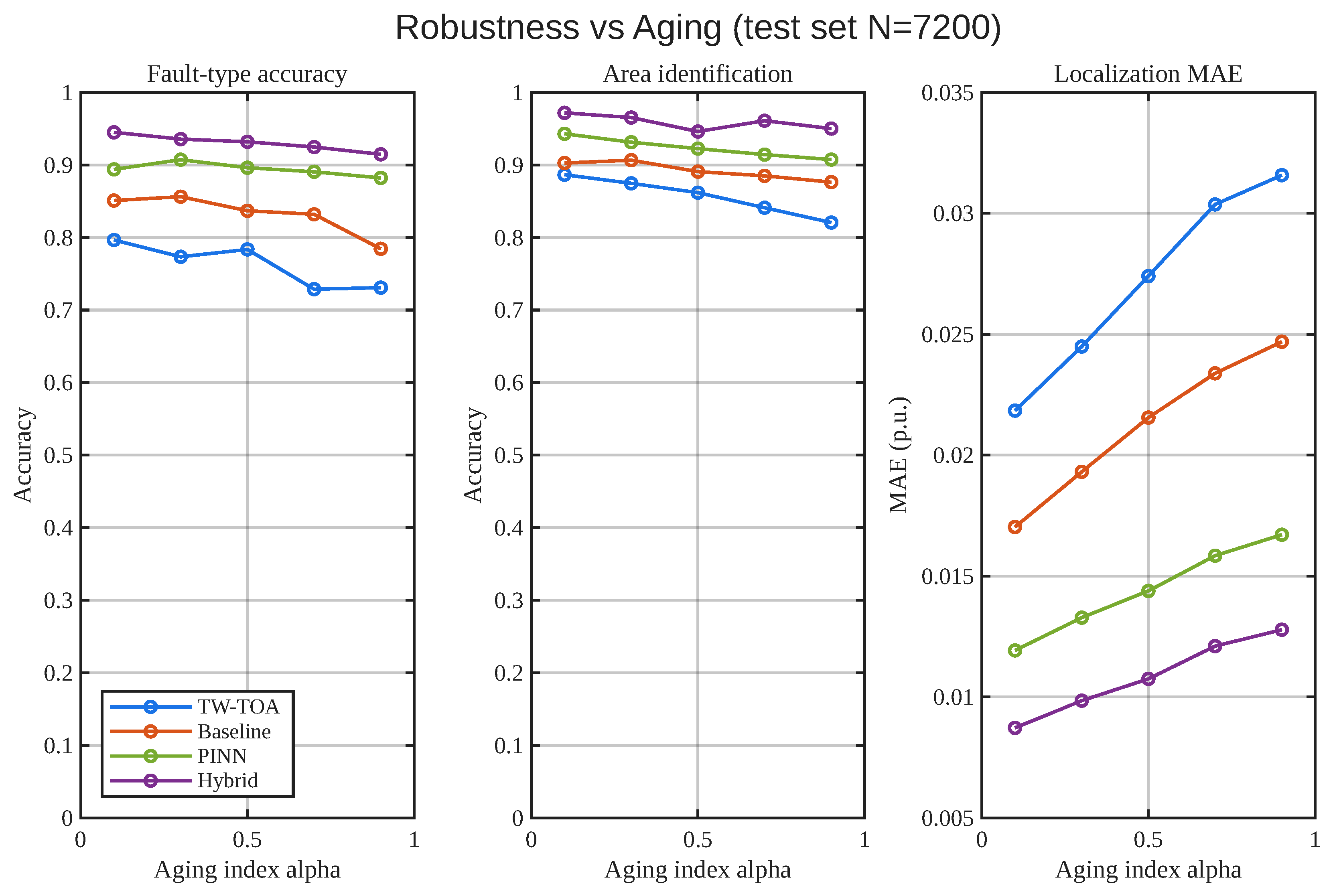
Binned robustness versus normalized aging-stress index on the test set: fault-type accuracy, area-identification accuracy, and localization MAE. Increasing aging degrades all models, whereas the Hybrid model shows the smallest performance degradation, indicating improved robustness to aging-driven propagation effects.
Figure 18.
Binned robustness versus normalized aging-stress index on the test set: fault-type accuracy, area-identification accuracy, and localization MAE. Increasing aging degrades all models, whereas the Hybrid model shows the smallest performance degradation, indicating improved robustness to aging-driven propagation effects.
Figure 19.
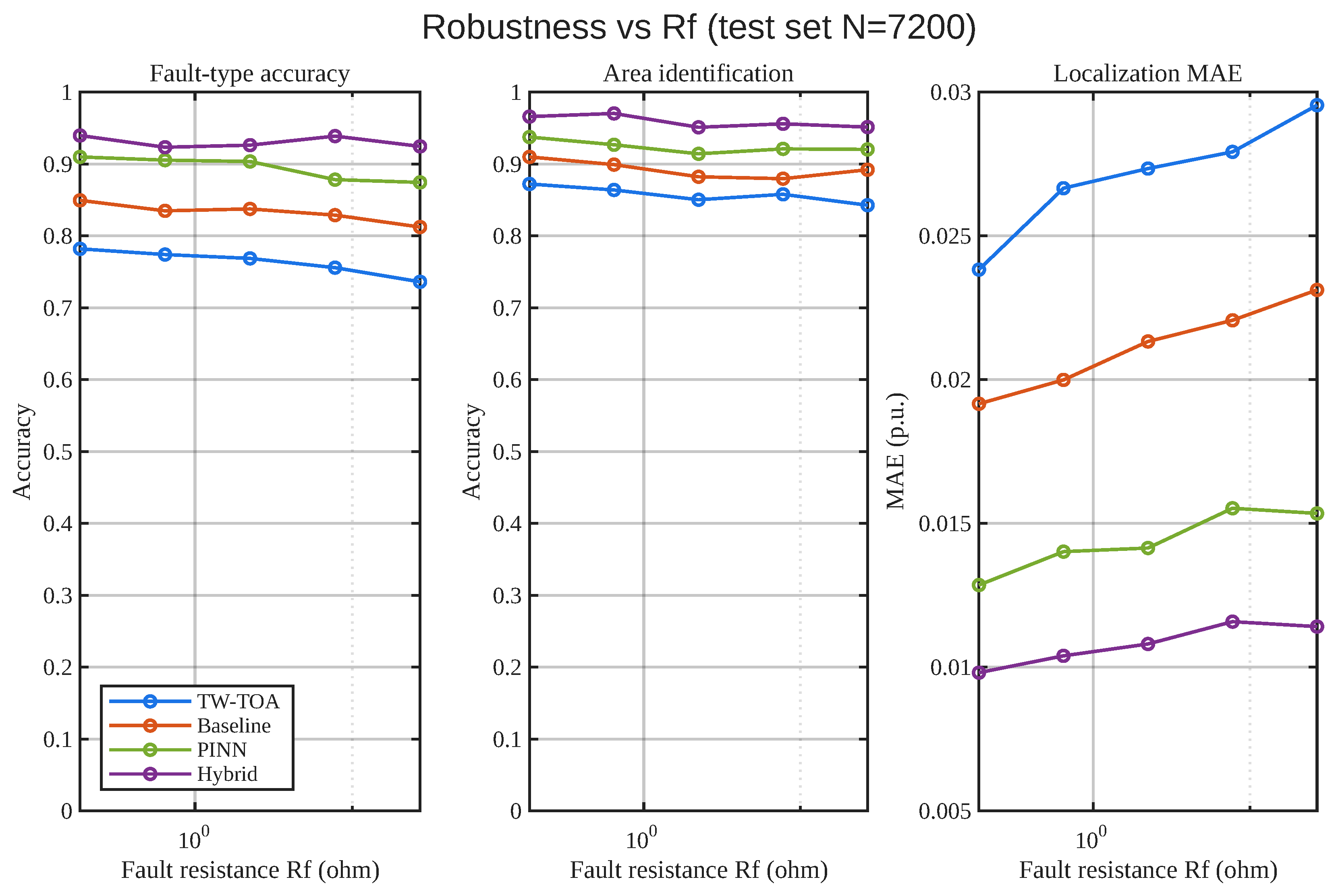
Binned robustness versus fault resistance on the test set: fault-type accuracy, area-identification accuracy, and localization MAE. Increasing weakens transient signatures and degrades performance for all models; the Hybrid model remains the most stable across the evaluated range.
Figure 19.
Binned robustness versus fault resistance on the test set: fault-type accuracy, area-identification accuracy, and localization MAE. Increasing weakens transient signatures and degrades performance for all models; the Hybrid model remains the most stable across the evaluated range.
Figure 20.
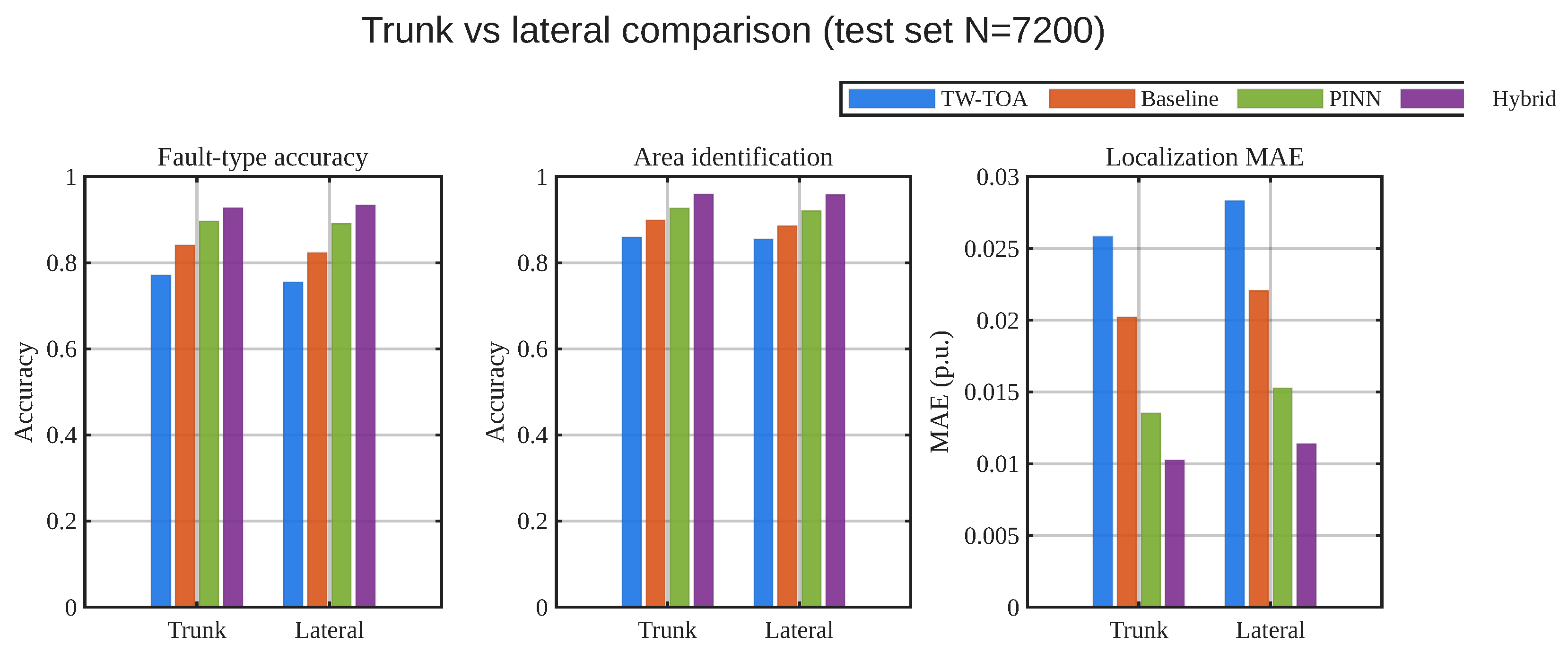
Topology-conditioned performance on the test set (): fault-type accuracy, area-identification accuracy, and localization MAE for trunk and lateral faults. Lateral events are more challenging due to additional branching effects, but the Hybrid model maintains superior performance in both regimes.
Figure 20.
Topology-conditioned performance on the test set (): fault-type accuracy, area-identification accuracy, and localization MAE for trunk and lateral faults. Lateral events are more challenging due to additional branching effects, but the Hybrid model maintains superior performance in both regimes.
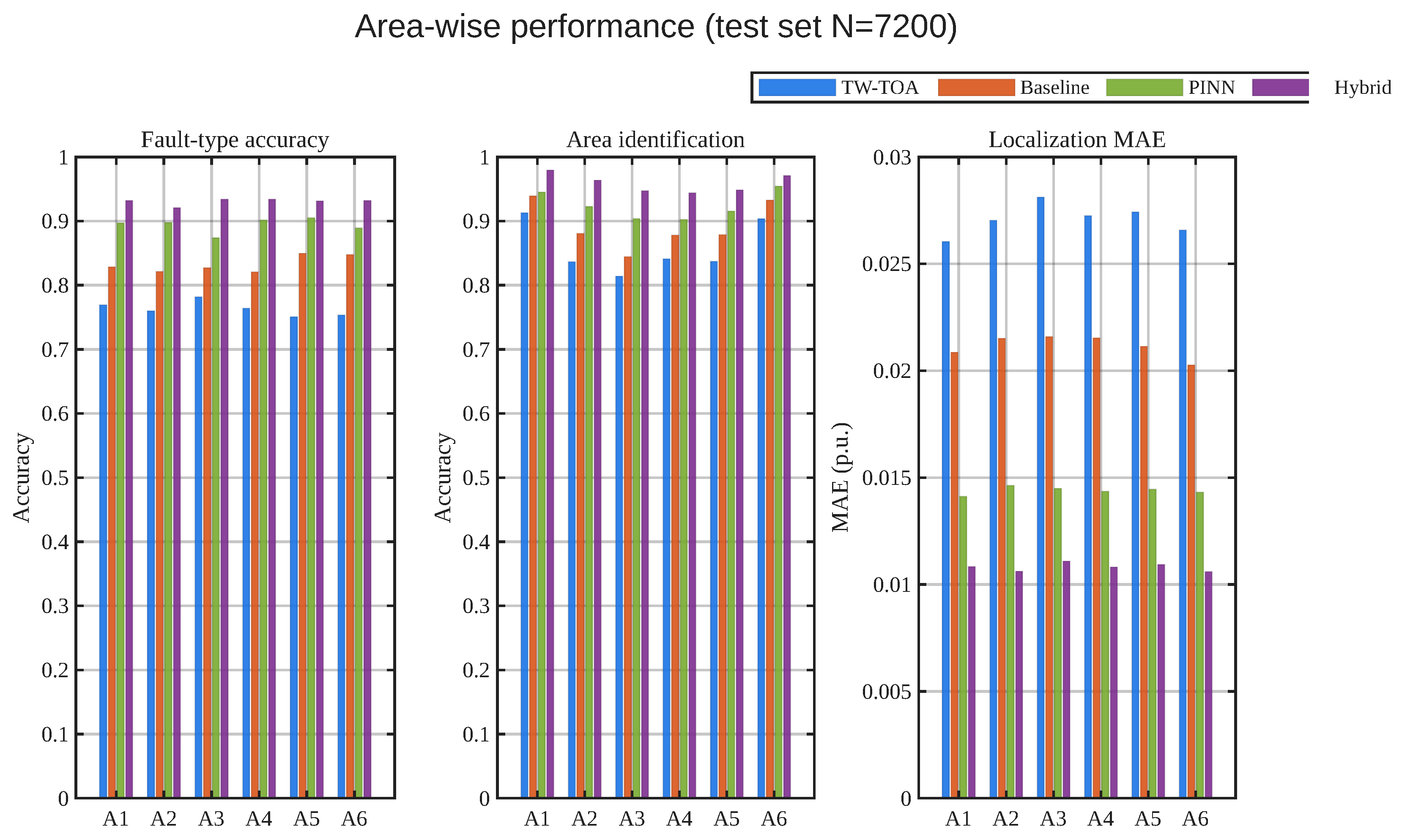
Figure 21.
Area-wise test-set performance for feeder partitions –: fault-type accuracy, area-identification accuracy, and localization MAE. The results show the influence of the area-dependent sensing geometry and branching structure on diagnostic performance.
Figure 21.
Area-wise test-set performance for feeder partitions –: fault-type accuracy, area-identification accuracy, and localization MAE. The results show the influence of the area-dependent sensing geometry and branching structure on diagnostic performance.
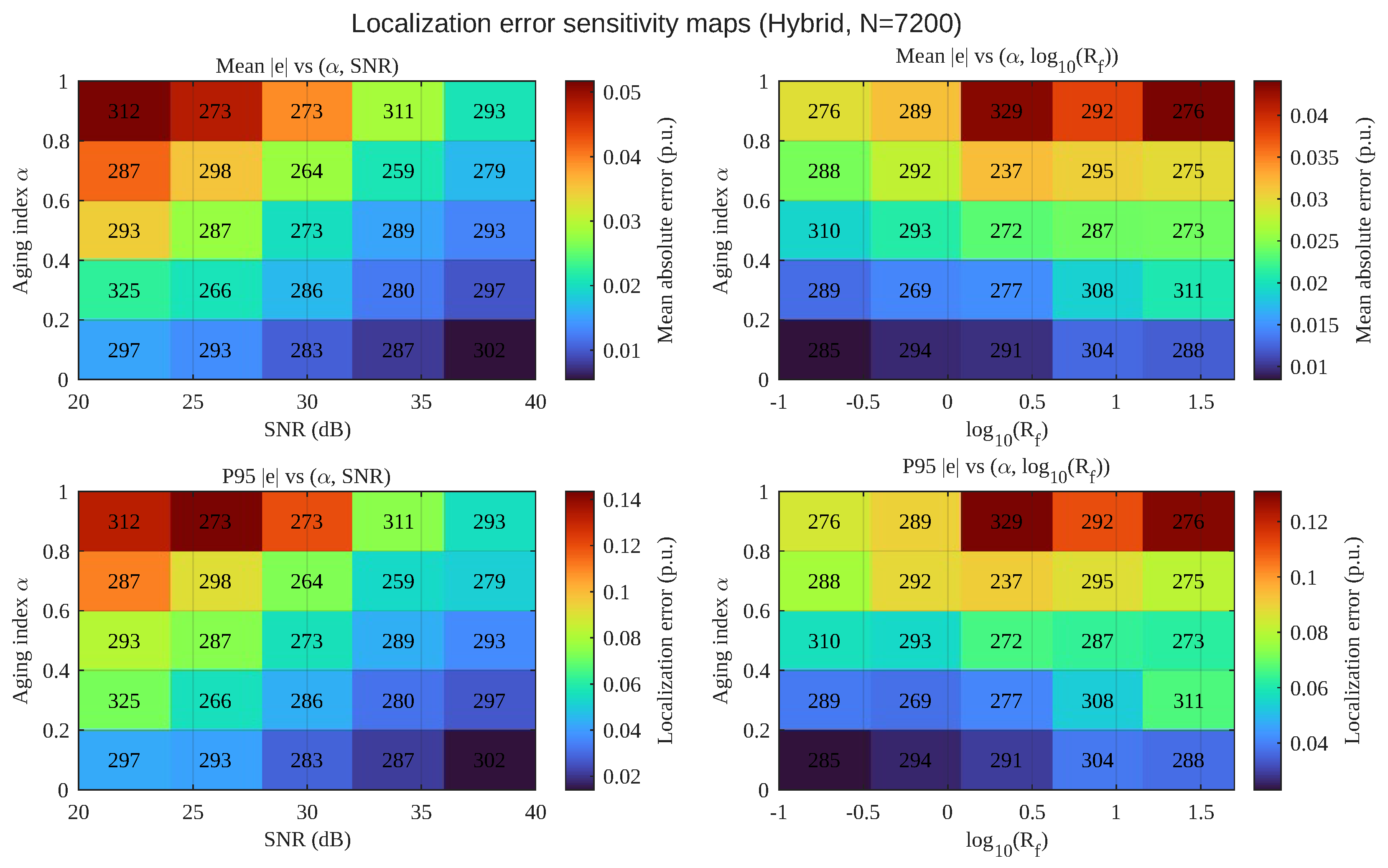
Figure 22.
Hybrid localization error sensitivity maps on the test set: binned mean absolute error (top row) and binned 95th-percentile absolute error (bottom row) as functions of and . Numbers inside cells denote per-bin sample counts, allowing verification that high-error regions are supported by adequate sample coverage.
Figure 22.
Hybrid localization error sensitivity maps on the test set: binned mean absolute error (top row) and binned 95th-percentile absolute error (bottom row) as functions of and . Numbers inside cells denote per-bin sample counts, allowing verification that high-error regions are supported by adequate sample coverage.
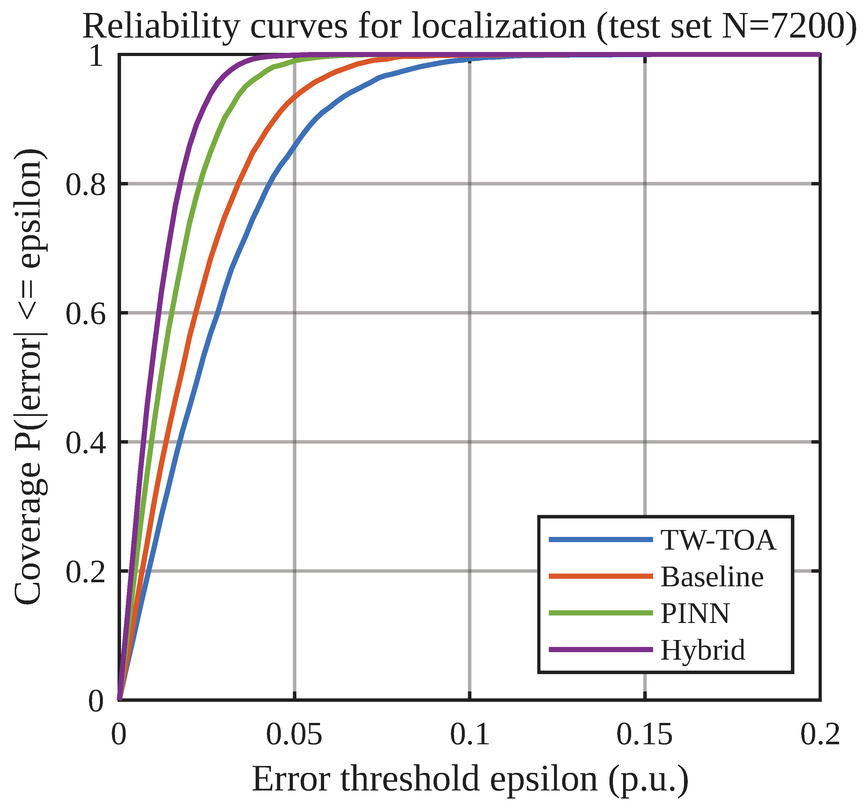
Figure 23.
Localization reliability curves on the test set: empirical coverage as a function of tolerance . Faster-rising curves indicate a higher probability of satisfying strict localization bounds. The Hybrid model achieves uniformly higher coverage across tolerances, indicating improved reliability.
Figure 23.
Localization reliability curves on the test set: empirical coverage as a function of tolerance . Faster-rising curves indicate a higher probability of satisfying strict localization bounds. The Hybrid model achieves uniformly higher coverage across tolerances, indicating improved reliability.
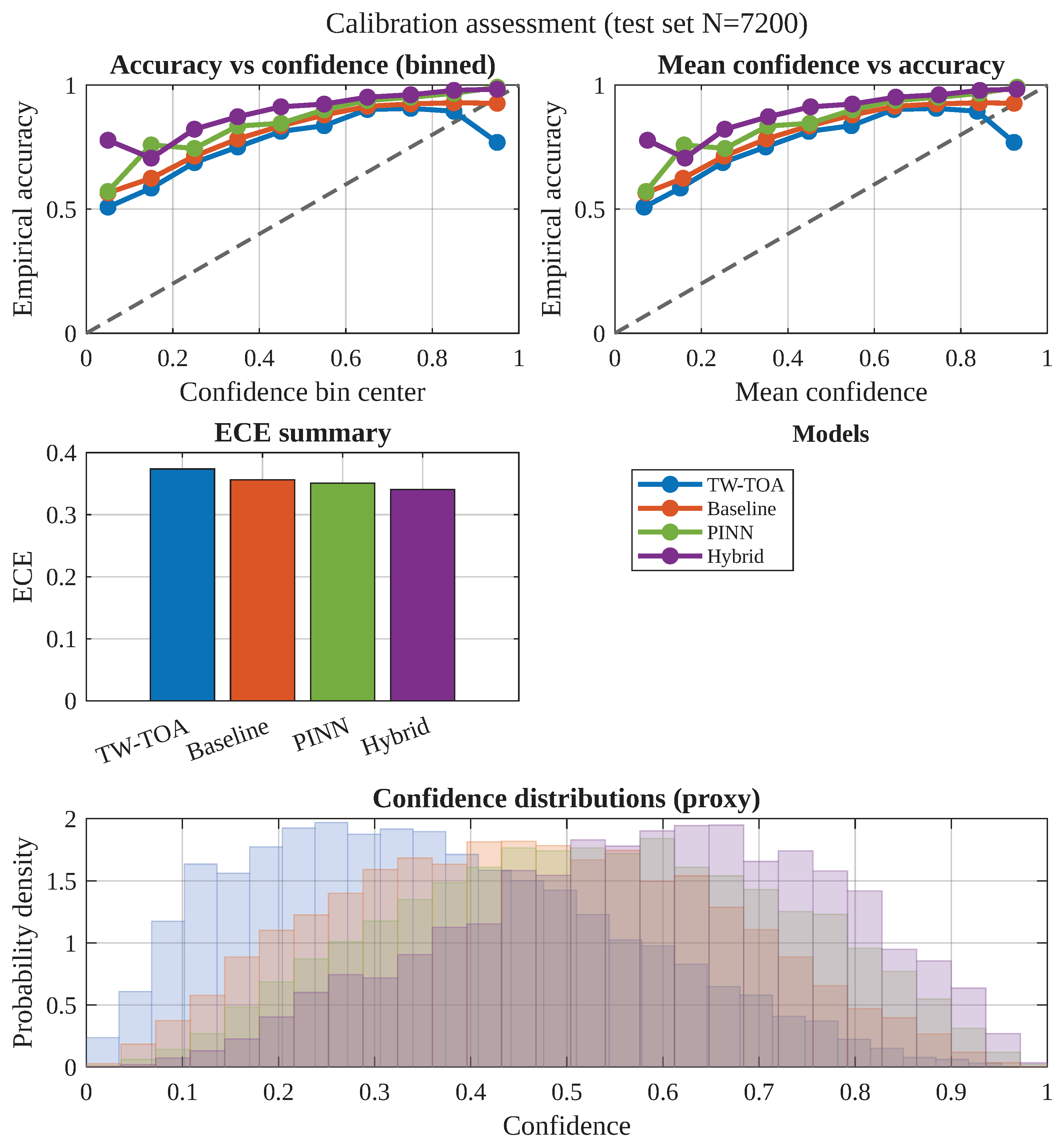
Figure 24.
Calibration assessment on the test set. The top-left and top-right panels show binned empirical accuracy and reliability results, respectively, and the middle-left panel reports expected calibration error. For the learning-based models, these three panels are calculated from the fault-type probabilities produced by the trained networks. The TW-TOA traces and the bottom confidence-density panel are proxy visualizations because the deterministic TW-TOA implementation does not produce native class probabilities and complete per-sample confidence distributions were not retained. Proxy elements are included only for qualitative context and are excluded from the quantitative calibration conclusions.
Figure 24.
Calibration assessment on the test set. The top-left and top-right panels show binned empirical accuracy and reliability results, respectively, and the middle-left panel reports expected calibration error. For the learning-based models, these three panels are calculated from the fault-type probabilities produced by the trained networks. The TW-TOA traces and the bottom confidence-density panel are proxy visualizations because the deterministic TW-TOA implementation does not produce native class probabilities and complete per-sample confidence distributions were not retained. Proxy elements are included only for qualitative context and are excluded from the quantitative calibration conclusions.
Figure 25.
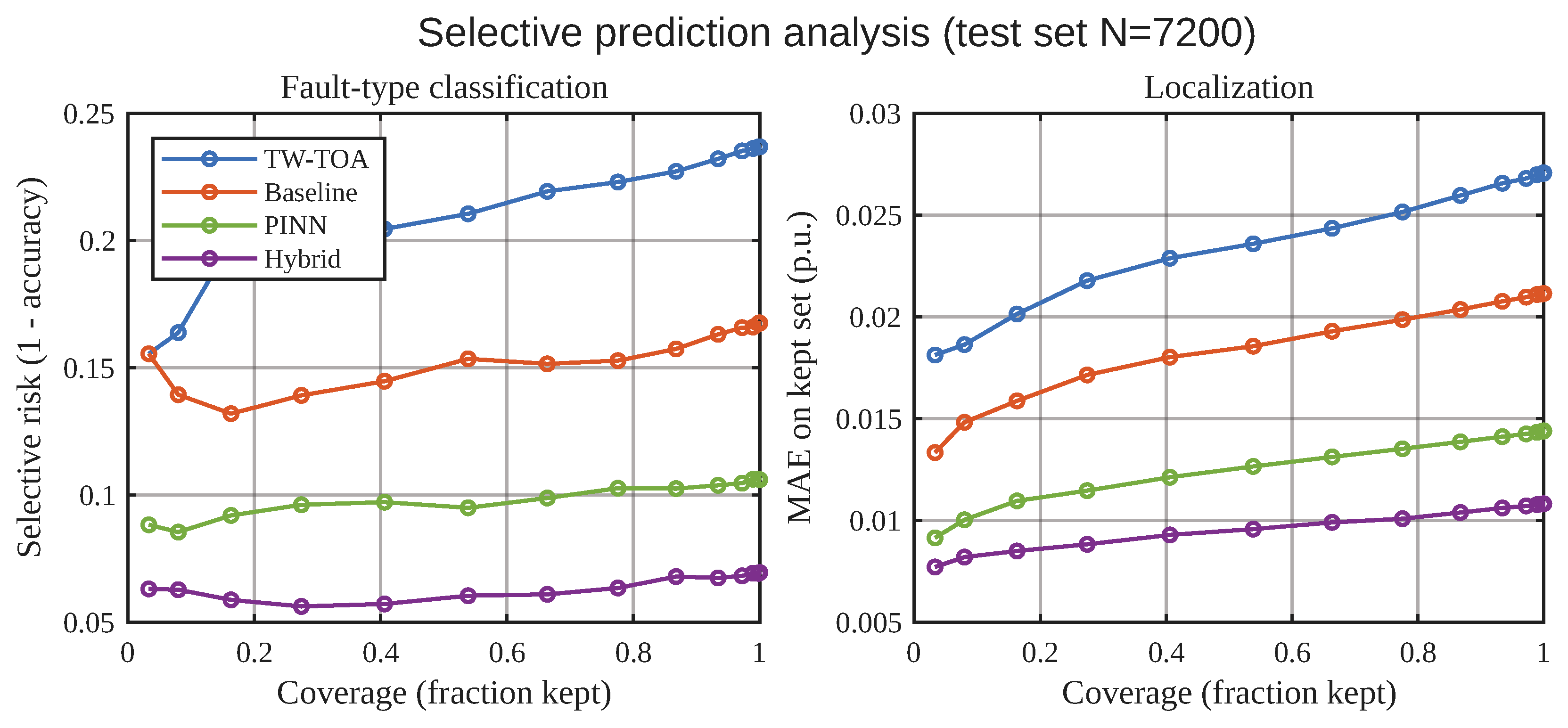
Selective prediction analysis on the test set. The left panel reports classification selective risk, and the right panel reports localization MAE over the retained subsets. For the learning-based configurations, samples are ranked using the maximum fault-type probability for classification and the maximum feeder-area probability for localization. The TW-TOA trace is shown only as a qualitative reference because TW-TOA does not provide native probabilistic confidence outputs.
Figure 25.
Selective prediction analysis on the test set. The left panel reports classification selective risk, and the right panel reports localization MAE over the retained subsets. For the learning-based configurations, samples are ranked using the maximum fault-type probability for classification and the maximum feeder-area probability for localization. The TW-TOA trace is shown only as a qualitative reference because TW-TOA does not provide native probabilistic confidence outputs.
Figure 26.
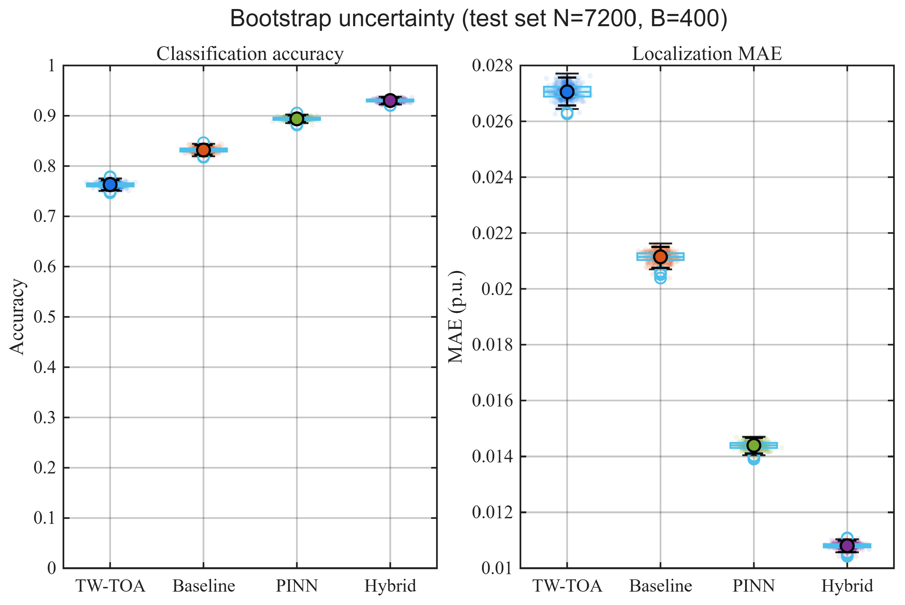
Bootstrap distributions on the test set: classification accuracy (left) and localization MAE (right) across bootstrap resamples. Markers indicate medians and intervals represent empirical percentile ranges.
Figure 26.
Bootstrap distributions on the test set: classification accuracy (left) and localization MAE (right) across bootstrap resamples. Markers indicate medians and intervals represent empirical percentile ranges.
Figure 27.
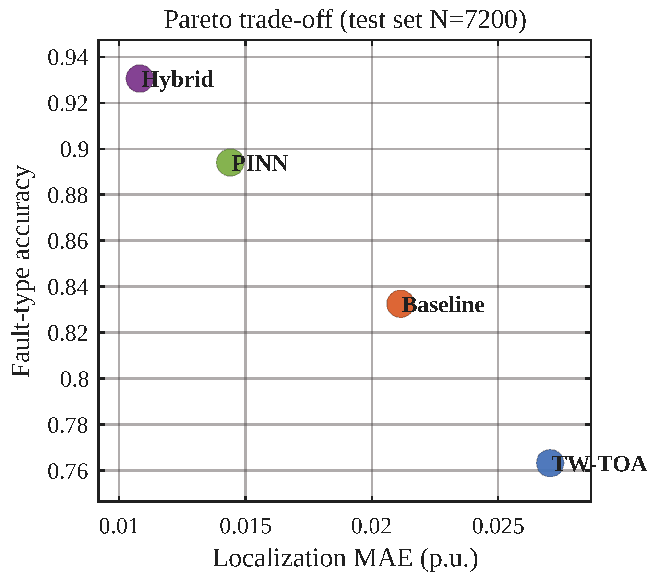
Pareto representation of fault-type accuracy versus localization MAE on the test set. Each point corresponds to one model. Points closer to the upper-left region indicate higher classification accuracy and lower localization error.
Figure 27.
Pareto representation of fault-type accuracy versus localization MAE on the test set. Each point corresponds to one model. Points closer to the upper-left region indicate higher classification accuracy and lower localization error.
Figure 28.
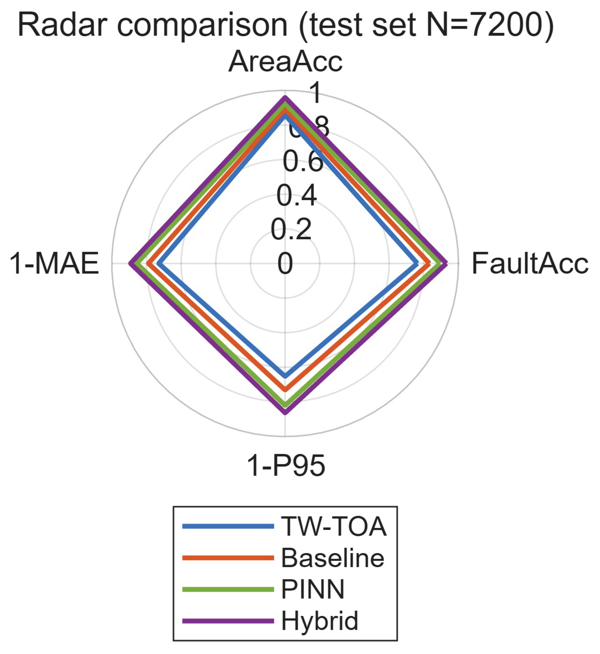
Radar comparison across normalized objectives with larger values indicating better performance on all axes: fault-type accuracy, area-identification accuracy, inverse localization MAE, and inverse localization P95. Normalization ensures consistent interpretation across metrics.
Figure 28.
Radar comparison across normalized objectives with larger values indicating better performance on all axes: fault-type accuracy, area-identification accuracy, inverse localization MAE, and inverse localization P95. Normalization ensures consistent interpretation across metrics.
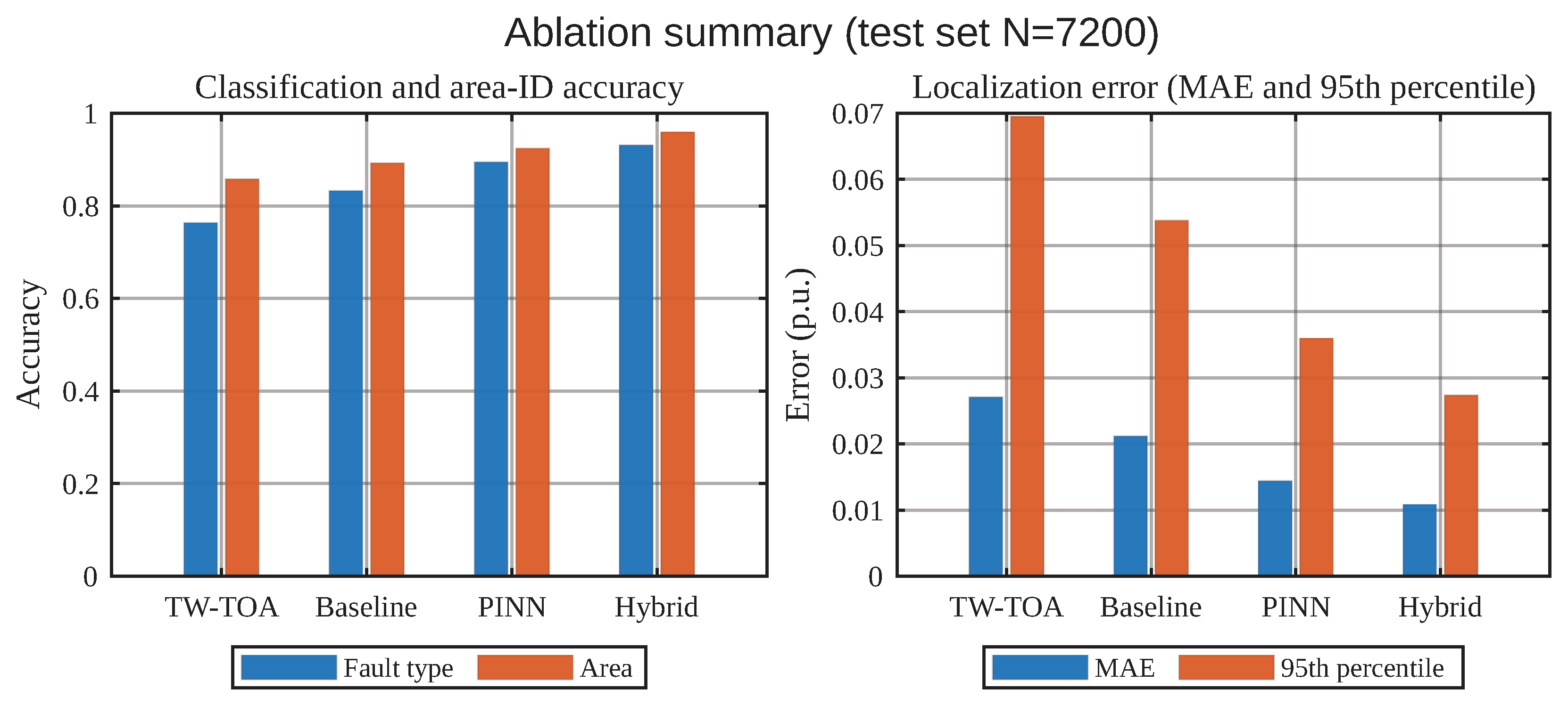
Figure 29.
Integrated-configuration performance summary on the test set. The panels compare fault-type and area-identification accuracies, localization MAE, and localization P95 for TW-TOA, Baseline, PINN, and Hybrid. The figure compares complete diagnostic configurations and should not be interpreted as a component-wise ablation of the Hybrid architecture.
Figure 29.
Integrated-configuration performance summary on the test set. The panels compare fault-type and area-identification accuracies, localization MAE, and localization P95 for TW-TOA, Baseline, PINN, and Hybrid. The figure compares complete diagnostic configurations and should not be interpreted as a component-wise ablation of the Hybrid architecture.
Table 1.
Interpretation of the aging-sensitivity coefficients used in the controlled simulation domain.
Table 1.
Interpretation of the aging-sensitivity coefficients used in the controlled simulation domain.
| Coeff. | Modeled Effect | Selection Criterion |
|---|
| Increase of effective series losses. | Chosen to produce monotonic loss increase while preserving positive series resistance. |
| Change in effective magnetic coupling and propagation characteristics. | Chosen as a bounded perturbation of the nominal inductive matrix without altering its coupling structure. |
| Reduction of effective capacitive behavior associated with dielectric degradation. | Chosen with to ensure remains nondegenerate for all . |
| Increase of dielectric leakage and shunt losses. | Chosen to stress attenuation and damping effects while preserving a physically admissible shunt conductance. |
Table 2.
Methodological hierarchy of the evaluated diagnostic configurations.
Table 2.
Methodological hierarchy of the evaluated diagnostic configurations.
| Configuration | Diagnostic Principle | Use of Physics | Role in the Evaluation |
|---|
| TW-TOA | Classical traveling-wave time-of-arrival estimation based on detected transient wavefronts. | Uses propagation-time interpretation and assumed wave velocity, but no learned representation. | Provides a physically interpretable reference for conventional TW-based localization. |
| Baseline | Supervised learning from the same transient time–frequency representation used by the learning-based models. | No explicit dynamic residual is imposed; equivalently, the physics-regularization weight is set to . | Isolates the performance of purely data-driven representation learning under the same dataset split and task definitions. |
| PINN | Physics-regularized learning using the same supervised task structure and an additional dynamic consistency penalty. | Uses the aging-aware cable matrices to construct during training. | Isolates the contribution of physics-consistency regularization relative to the purely data-driven baseline. |
| Hybrid | Complete proposed formulation combining transient time–frequency learning, aging-conditioned physics consistency, area-aware localization, multi-sensor information, and task-specific explanation. | Uses the aged cable model to regularize learning and to structure the diagnostic pipeline under parameter drift. | Evaluates the full integrated method proposed in this paper for simultaneous fault-type classification, area identification, and continuous fault localization. |
Table 3.
Case-study topology and simulation configuration.
Table 3.
Case-study topology and simulation configuration.
| Item | Value/Description |
|---|
| Network type | Synthetic branched underground distribution feeder |
| Electrical representation | Cascaded -section underground-cable model |
| Numerical tool | MATLAB 2025b transient simulation |
| Number of trunk nodes | 13, from to |
| Number of laterals | 6, including one double-lateral junction at |
| Feeder partitions | non-overlapping areas |
| Synchronized sensors | |
| Sensing configuration | Multi-ended, area-dependent transient monitoring |
| Signal channels | Three-phase voltages and currents at each sensor |
| Sampling rate | |
| Transient window | |
| Operating-point variability | Load scaling |
| Cable parameters | Nominal , , , perturbed by as in Section 3.7 |
Table 4.
Sensor subsets used for each area in the area-wise localization strategy.
Table 4.
Sensor subsets used for each area in the area-wise localization strategy.
| Area | Sensor Subset |
|---|
| |
| |
| |
| |
| |
| |
Table 5.
Simulation scenario parameter ranges used for dataset generation.
Table 5.
Simulation scenario parameter ranges used for dataset generation.
| Parameter | Minimum | Maximum | Unit |
|---|
| Fault resistance | 0.1 | 50 | |
| Fault location in section | 0.05 | 0.95 | – |
| Normalized aging-stress index | 0 | 1 | – |
| Load scaling | 0.80 | 1.20 | – |
| SNR | 20 | 40 | dB |
Table 6.
Dataset composition and interpretation of the large-case-study split.
Table 6.
Dataset composition and interpretation of the large-case-study split.
| Subset | Samples | Stratification | Role and Domain |
|---|
| Training | 25,200 | Uniform by area and fault type | Model fitting using the complete prescribed ranges of aging, fault resistance, loading, noise, and fault location. |
| Validation | 3600 | Uniform by area and fault type | Hyperparameter selection and training monitoring within the same simulation domain. |
| Test | 7200 | Uniform by area and fault type | Held-out event-level evaluation within the same simulator and parameter ranges; not a grouped or out-of-domain test. |
Table 7.
Validation scope and practical deployment assumptions of this paper.
Table 7.
Validation scope and practical deployment assumptions of this paper.
| Aspect | Assumption in This Study | Requirement Before Field Deployment |
|---|
| Data source | Controlled simulation using the cascaded -section underground-cable model. | Validation with independent electromagnetic-transient simulations and, where available, laboratory or field transient records. |
| Measurement chain | Ideal synchronized voltage/current channels with additive noise set by the prescribed SNR range. | Sensitivity analysis including sensor bandwidth, timing skew, filtering, saturation, recorder resolution, and channel-dependent transfer functions. |
| Cable aging | Normalized aging-stress index used to induce monotonic drift in cable parameters. | Calibration of or replacement by measured condition indicators, such as thermal history, dielectric loss, partial-discharge indicators, or asset-specific diagnostic data. |
| Cable parameters | Nominal matrices perturbed according to the aging parameterization. | Assessment under uncertain nominal parameters, spatially heterogeneous cable sections, and frequency-dependent dielectric behavior. |
| Performance claims | Comparative simulation-based performance under identical sampled scenarios for all methods. | Cross-domain validation to quantify degradation when the training and testing domains differ in simulator, sensor model, topology, operating conditions, or aging mechanism. |
Table 8.
Evaluation protocol used for the reported test-set analysis.
Table 8.
Evaluation protocol used for the reported test-set analysis.
| Item | Value/Description |
|---|
| Test-set size | held-out simulated events |
| Stratification | By feeder area and fault type |
| Evaluated configurations | TW-TOA, Baseline, PINN, and Hybrid |
| Discrete tasks | Fault-type classification and feeder-area identification |
| Continuous task | Normalized fault-location estimation |
| Classification metrics | Accuracy, precision, recall, and F1-score |
| Localization metrics | MAE, P95, empirical coverage, and bootstrap uncertainty |
| Robustness variables | SNR, normalized aging-stress index , fault resistance , and topology subset |
| Interpretability output | Time–frequency attribution illustration and model-native attribution-validation protocol |
Table 9.
Test-set performance summary across fault-type classification, area identification, and localization. Localization errors are expressed in per-unit distance.
Table 9.
Test-set performance summary across fault-type classification, area identification, and localization. Localization errors are expressed in per-unit distance.
| Model | Fault Acc. | Area Acc. | MAE | P95 |
|---|
| TW-TOA | 0.76 | 0.86 | 0.027 | 0.069 |
| Baseline | 0.83 | 0.90 | 0.021 | 0.054 |
| PINN | 0.89 | 0.93 | 0.014 | 0.036 |
| Hybrid | 0.93 | 0.96 | 0.011 | 0.027 |
Table 10.
Relative gains of the Hybrid model with respect to each reference configuration. “pp” denotes percentage points.
Table 10.
Relative gains of the Hybrid model with respect to each reference configuration. “pp” denotes percentage points.
| Hybrid vs. Reference | Fault
(pp) | Area
(pp) | MAE Red.
(%) | P95 Red.
(%) |
|---|
| TW-TOA | +17.0 | +10.0 | 59.3 | 60.9 |
| Baseline | +10.0 | +6.0 | 47.6 | 50.0 |
| PINN | +4.0 | +3.0 | 21.4 | 25.0 |
Table 11.
Bootstrap summary on the test set: median and empirical percentile confidence intervals for classification accuracy and localization MAE.
Table 11.
Bootstrap summary on the test set: median and empirical percentile confidence intervals for classification accuracy and localization MAE.
| Model | Accuracy (Median [95% CI]) | MAE (p.u.) (Median [95% CI]) |
|---|
| TW-TOA | 0.76 [0.75, 0.77] | 0.027 [0.0265, 0.0275] |
| Baseline | 0.83 [0.82, 0.84] | 0.021 [0.0208, 0.0216] |
| PINN | 0.89 [0.88, 0.90] | 0.014 [0.0140, 0.0146] |
| Hybrid | 0.93 [0.92, 0.94] | 0.011 [0.0105, 0.0111] |