Load Frequency Regulation of Renewable-Integrated Power System Using Novel Fractional and Degree of Freedom-Based Controller with Real-Time Validation

Abstract

Microgrid integration introduces fast, stochastic disturbances that challenge frequency stability. This paper presents a two-degree-of-freedom fractional-order proportional tilt integral derivative plus one controller (2DOF-FOPTID+1) tuned with a Modified Walrus Optimization Algorithm (MWA) to mitigate frequency deviations while preserving tracking performance. The novelty lies in jointly deploying a 2DOF-FOPTID+1 structure for decoupled tracking and regulation, an MWA-based tuning strategy tailored for resilient frequency control, and the explicit use of aggregated electric vehicles as fast distributed storage to damp frequency and tie-line power excursions; hardware-in-the-loop validation using an OPAL-RT platform is included to demonstrate practical feasibility. The controller is evaluated under step and random load variations, and robustness is examined for $\pm 25\%$ parameter perturbations and stochastic renewable inputs. Compared with the strong baselines PID, FOPID, 2DOF-PID, and FOPTID, the proposed approach reduces settling time by up to 39.27% and lowers peak-to-peak frequency deviation by about 20.88% under these operating scenarios, indicating a practical and effective solution for enhancing frequency resilience in microgrid-integrated power systems.

1. Introduction

Microgrids have emerged as a vital component of modern power systems, offering decentralized generation, enhanced resilience, and seamless integration of renewable energy sources [1,2,3]. Typically comprising localized units such as solar panels, wind turbines [4], and energy storage systems [5], microgrids [6] significantly reduce environmental impact. However, the inherent intermittency of renewables introduces new challenges to frequency stability, particularly under variable demand and isolated operation. Variations in solar irradiance, wind availability, and consumer load often lead to frequency deviations, which must be effectively managed to ensure reliable operation.

To address this, load frequency control (LFC) plays a key role in maintaining the power balance between generation and consumption and in regulating tie-line power exchanges. Traditionally, proportional–integral–derivative (PID) controllers [7] have been widely used due to their simplicity and reliable performance in steady operating conditions. Nevertheless, their effectiveness diminishes in modern power systems characterized by nonlinear dynamics, stochastic variations, and parameter uncertainties. To overcome these limitations, researchers have investigated fractional-order and two-degree-of-freedom (2DOF) controllers as promising alternatives. Fractional-order PID (FOPID) controllers [8,9] offer enhanced flexibility and disturbance rejection by extending the control action into the fractional domain. Similarly, 2DOF-PID controllers [10,11] enable separate tuning for set-point tracking and disturbance rejection, thus, improving transient response. These principles have led to cascaded controller structures such as PI–PD [12,13], FOPI–FOPD [14,15], and more advanced configurations like 2DOF-FOPIDN–FOPDN [16], FOPI–FOPIDN [17], 2DOF(FOPI$\lambda$DN)–PDN [18], PI-(1+FOPID)  [19], and P-P-FOPID [20]. Hybrid variants, including TFODn–FOPI [21], 3DOF(FOPI)–FOPD [22], and 2DOF–PIDN–FOID [23], have demonstrated superior adaptability in microgrid and deregulated environments. However, the complex tuning requirements of these cascaded structures often hinder their real-time applicability. Alongside these efforts, several advanced control strategies have been proposed, including model predictive control (MPC)  [24], sliding mode controllers (SMC), and $H_{\infty }$ observer-based methods [25,26]. Other intelligent approaches such as neural networks [27], fuzzy logic [28], and adaptive controllers [29,30] have also gained attention. While these techniques offer robustness, learning capability, and theoretical guarantees, they are often limited by high computational complexity, the need for expert design, and difficulties in deployment under practical constraints.

Apart from the controller, a storage system supports enhancing the frequency regulation. A wide range of energy storage systems has been employed to support LFC, yet each comes with limitations. Pumped hydro energy storage, though effective, is geographically constrained and lacks rapid response capability [31]. Superconducting magnetic energy storage (SMES) systems offer fast dynamics but are expensive and require complex cryogenic infrastructure [32]. Supercapacitors have limited energy capacity, making them suitable only for short-duration events [33]. Flywheels, despite their quick response and high efficiency, suffer from mechanical wear and energy loss over time. Redox flow batteries are constrained by slow kinetics and high maintenance costs [34]. Moreover, the use of standalone EVs is often hindered by uncoordinated dispatch and stochastic behavior [35]. To overcome this, the integration of Electric Vehicle Aggregators (EVA) alongside optimized controllers has been shown to effectively reduce transient deviations in multi-area power grids [36]. However, with the increasing integration of renewable energy, coordinating distributed resources and electric vehicles is becoming increasingly important as a flexibility resource for power balancing, frequency support, and multi-area regulation [37,38,39]. Among the above literature few of the recent articles are summarized in

Table 1. Analysis on some recent literature.

Ref. No	System Used	Controller	Findings	Research Gaps
[13]	Single area LFC with non reheat and reheat units and multi source supply. Parameter variation up to $\pm 50\%$.	PI and PD in inner and outer loops tuned by a modified weighted geometric center on the stability boundary locus. Inner loop gain margin equals 1 and phase margin is ≈20°.	Reduces IAE, ISE, ITAE, settling time, and peak compared with cited PID. Robust to $\pm 50\%$ changes.	No two-area or tie-line study. Simulation only. Renewables and BESS not modeled.
[14]	Interconnected hydro thermal system under large disturbances.	FOPI and FOPD with a continuous filter. Parameters tuned with imperialist competitive algorithm with Levy mutation using ITAE objective.	Faster frequency recovery. In zone 1 the settling time decreases by 0.4 s versus TID and by 4.31 s versus PID and overshoot reduces by 33.3% and 71.4%.	Simulation only. Comparisons limited to PID and TID. No renewables or BESS.
[15]	Two-area thermal system with and without governor dead band and a three-area hydro thermal system with generation rate constraints. Also single and multi area multi source cases.	Cascaded FOPI and FOPD with fractional orders k and ℓ tuned by the dragonfly search algorithm using JITAE and ITAE on frequency and tie-line power deviations.	Lower JITAE and improved settling time, undershoot, and overshoot compared with DSA tuned FOPID and recent works.	Simulation only. HVDC and PEV not included. No renewables or BESS.
[17]	Two- and three-area systems with hydro, thermal, and renewable sources. Tests include step and random load with PV and wind, generation rate constraints, governor dead band, communication delays, and $\pm 50\%$ parameter changes.	Cascaded FOPI and FOPID with a derivative filter. Parameters tuned with an adaptive dynamic PSO variant named ADIWACO.	Lower ITAE and reduced frequency and tie-line power deviations. Robust under constraints and $\pm 50\%$ variations. Scales to larger systems.	Fixed gains that are not adaptive. Simulation only without hardware in the loop.
[21]	Islanded microgrid with renewable sources. Includes time delay nonlinearities, renewable fluctuations, parameter uncertainty, and cyber attack. Laboratory rapid control prototyping is used.	Multi stage fractional order controller with TFODn followed by FOPI. Tuned with prairie dog optimization.	Tracks the set point and remains robust under delays, renewable variability, and cyber attack. Real time tests show superior performance.	Islanded mode only with no grid connected or inter area study. No explicit battery model.
[23]	Two-area non reheat thermal system and two-area multi source thermal hydro gas system with OPAL RT hardware in the loop.	Two DOF PID with derivative filter and fractional order integral derivative part named 2DOF PIDN FOID. Tuned with differential evolution.	Outperforms GA, BFOA, hybrid BFOA PSO, Firefly, DE PID, and TLBO two DOF PID. Robust to $\pm 25\%$ changes and random loads. Hardware tests match simulations.	No renewables, EVs, or BESS. Communication delays and other constraints are not detailed.
[24]	Islanded VSC based microgrid with focus on primary control in outer and inner loops.	Cascaded model predictive control. The outer loop uses an MPC based virtual synchronous generator with direction aware objectives. The inner loop uses double vector finite set MPC.	Faster frequency dynamics and lower tracking error. Shown by simulation and experiments.	Inertia is fixed. Islanded mode only with no secondary or tertiary control. No explicit battery model.
[30]	Islanded microgrid with high penetration of distributed energy resources including synchronous units. Secondary control on the IEEE 34 bus system.	Distributed Lyapunov function based secondary control that uses distribution level PMU measurements of global active and reactive power. Average voltage converges to the reference. Parameters set by Lyapunov conditions.	Large reductions in frequency and voltage transients with accurate power sharing in simulations.	Simulation only. Periodic communications add overhead. Cyber resilience is future work. No battery modeling.
[31]	Isolated El Hierro system with diesel, wind, and pump storage hydropower with AGC and a flywheel energy storage plant.	Six flywheel governor control schemes named DB, DBV, PD, PDV, NLP, and NLPV. Tuning considers renewable mix, frequency impact, wear and tear, and cycle count.	Flywheel improves frequency quality. NLP and NLPV reduce average frequency deviation by up to 29% and 26%. State of charge aware schemes maintain state of charge and reduce wear and tear.	Simulation only with a single case. No comparison with battery or EV support. Communication and cyber issues are not addressed.
[33]	Single doubly fed induction generator operating at maximum power point with supercapacitor storage. Simulations and experiments.	Supercapacitor control provides virtual inertia and primary frequency regulation without deloading or pitch changes. Capacity is optimized for cost and efficiency.	Improved inertia and primary regulation while keeping MPPT energy capture. Supercapacitor efficiency is about 99.31% and cost is about 9% of a unit. Strong economic advantage over overspeed reserve.	Single turbine study with no wind farm or system level tests. Communication and cyber topics are not discussed.
[35]	Isolated hybrid grids. Compares EV support with SMES, capacitive storage, and redox flow batteries under fixed and variable loads.	PSO tuned FOPID for EV converters with a modified virtual rotor concept that adds virtual inertia and damping.	Dynamic undershoot improves by more than 50% and steady state offset by more than 20%. FOPID with or without MVRC shows more than 75% improvement. Tracking is similar to double integral sliding mode but with fewer sensors.	Simulation only. EV state of charge and availability and communication delays are not addressed.
[40]	Three-area hydro thermal system with an asynchronous HVDC link and energy storage based inertia emulation. Includes random load pattern and communication delays that are constant and variable. OPAL RT is used.	TIDD two secondary controller tuned by the artificial hummingbirds algorithm. Compared with IDD PID, TID, and PID controllers and with BSA and HHO optimizers.	TIDD two with AHA gives the best dynamics. SMES performs better than battery and ultracapacitor for inertia emulation. Hardware results agree with MATLAB and eigenvalue trends show scalability.	No renewable generation is modeled. No field deployment beyond hardware in the loop.
[41]	Multi area restructured thermal hydro gas system with poolco, bilateral, and contract violation scenarios. Two-area case with generation rate constraints and an HVDC tie-line with inertia emulation and an extension to a three-area case with distributed generation and EV services.	OVPLA optimized cascaded controller named CC with two DOF PI followed by PD with a filter.	Faster disturbance rejection. The HVDC with inertia emulation improves frequency regulation. The approach manages contract violations and performs well on a three-area system. Superior to prior literature.	Primarily simulation. Communication delays are not analyzed. Battery modeling is not explicit.
[10]	Three-area unequal LFC with nonlinearities and an extension to a four-area system.	Two DOF PID tuned by the improved sine cosine algorithm. Compared with PID and FOPID and with SCA, SSA, ALO, and PSO. Wilcoxon signed rank tests are used over 20 runs.	Best convergence and objective values. Two DOF PID reduces settling time and undershoot across scenarios with statistically significant gains.	Simulation only. No modeling of renewables or energy storage.
[42]	One area multi source thermal hydro gas system extended to a two-area case with a linear model and with governor dead band and generation rate constraints. AGC with capacitive energy storage.	FOPTID plus one tuned by the global neighbourhood algorithm. Compared with DE, TLBO, hSFS PS, and IPSO and PFA tuned PID, TID, FOPID, and FOTID.	With CES the system shows large reductions in settling time, undershoot, overshoot, and ITAE. Robust to $\pm 25\%$ parameter changes and tie-line trips. Bode analysis supports stability.	Simulation only. No renewables or EVs. Communication delays are not considered. The energy storage comparison is limited to CES.

.

Based on the surveyed literature, while advanced controllers and various energy storage systems have shown potential in enhancing frequency regulation, they continue to suffer from practical limitations such as complex tuning procedures, reduced adaptability under stochastic disturbances, limited scalability, and challenges in real-time deployment. Moreover, conventional storage units such as SMES, redox flow batteries, and flywheels either incur high costs, suffer from physical degradation, or lack coordination flexibility. The increasing availability and controllability of EVs offer a promising alternative; however, most existing approaches treat EVs as isolated units without considering their aggregated potential. This creates a gap in fully exploiting EV fleets as coordinated, scalable, and responsive storage assets for grid frequency support. To address these limitations, the present study proposes a comprehensive solution that combines a two-degree-of-freedom fractional-order proportional–integral–derivative plus one (2DOF-FOPTID+1) controller, offering superior disturbance rejection and tuning flexibility, with an AEV model that acts as a distributed, controllable, and high-response energy storage system for frequency regulation in microgrid-integrated power systems. The key contributions of this work are listed below.

• A new two-degree-of-freedom fractional-order controller (2DOF-FOPTID+1) is proposed for a two-area power system integrated with electric vehicles. Compared to standard controllers, this new design provides much better setpoint tracking and faster disturbance rejection when dealing with the unpredictable nature of solar, wind, and electric vehicle loads.
• The robust stability of the proposed controller is mathematically proven by deriving the eigenvalues of the considered MIP. This guarantees that the system remains strictly stable even under severe grid disturbances compared with the state of art controllers.
• A Modified Walrus Optimization Algorithm (MWA) is introduced to tune the controller parameters. Testing shows that MWA is superior to recent existing methods (like the Sea Horse, Mountain Gazelle, and standard Walrus optimizers) because it achieves the lowest error (ITAE) and finds much more stable control settings.
• The superiority and practical value of the proposed method are confirmed through real-time hardware testing using the OPAL-RT platform. This hardware-in-the-loop validation proves that the new controller works reliably under real-world conditions, bridging the gap between theoretical math and practical grid deployment.

The later part of this article illustrates the detailed description of the two-area power system in Section 2, including its mathematical modeling and state-space representation. Section 3 presents the proposed controller along with the optimization approach adopted for parameter tuning. Section 4 provides an in-depth analysis of the system’s performance under various loading conditions and different renewable input signals and includes validation of the results using the OPAL-RT platform. Section 5 concludes the article by summarizing the key findings.

2. State-Space Analysis of the Considered System

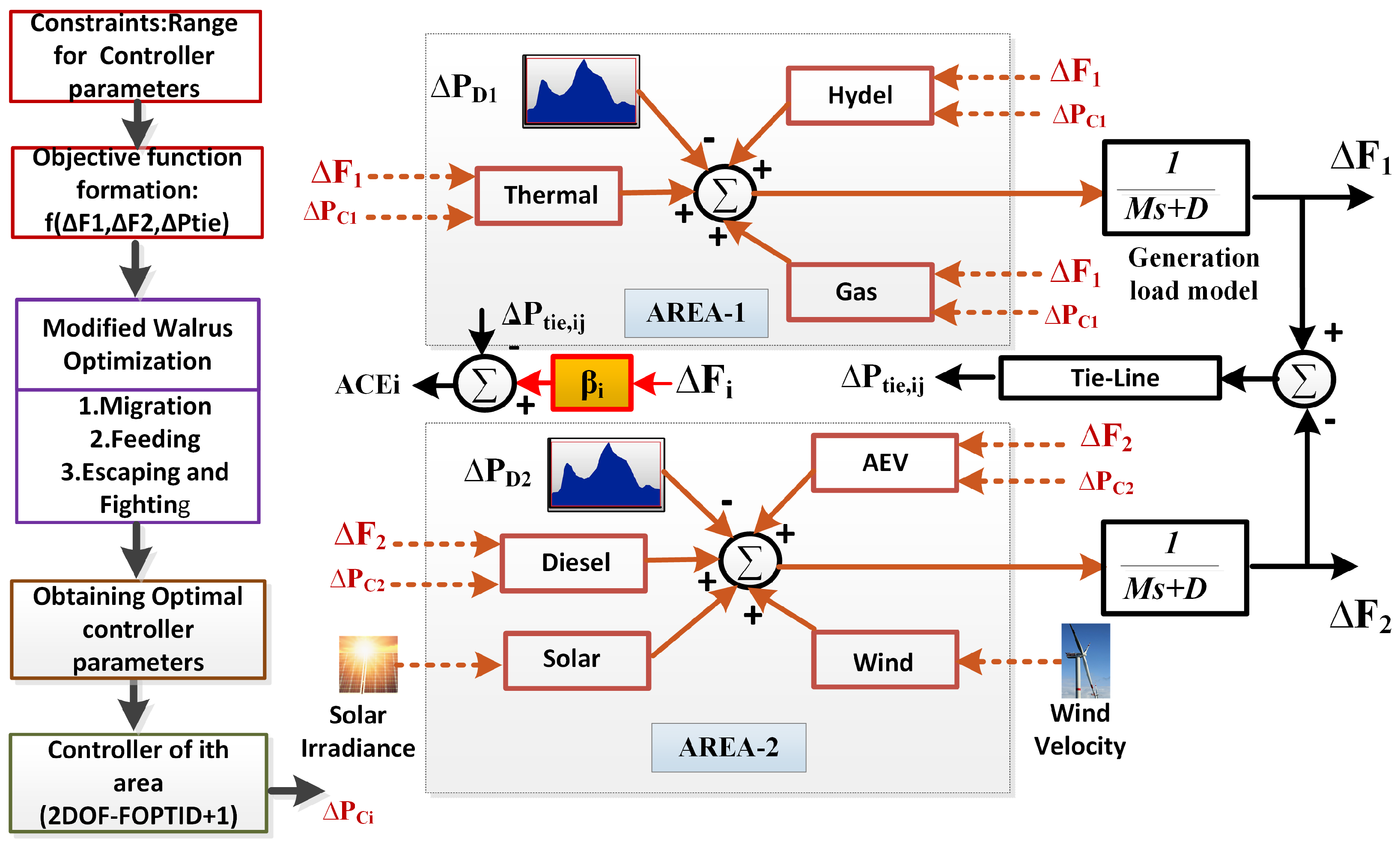
In this study, a hybrid two-area power system incorporating both conventional and renewable energy sources is considered, as illustrated in Figure 1. Area 1 represents the main grid with a total capacity of 1000 MW, consisting of thermal, hydel [40], and gas-based generation [43], ensuring high inertia and frequency stability. Area 2 is a microgrid with a total capacity of 110 MW, incorporating wind, solar [44], and aggregated EV storage [41]. The diesel generator serves as a backup, ensuring stability during low renewable generation. The interconnected system enables effective LFC by balancing the stability of conventional units with the flexibility of renewable and distributed energy resources.

Prior to deriving the state-space model, certain modeling assumptions are established. The system is assumed to be subjected to small load perturbations, which allows for the linearization of the highly non-linear power system dynamics around a nominal operating point. Furthermore, the primary speed control (governor droop characteristics) and the secondary supplementary control (ACE-based signals) are assumed to act linearly within operational limits.

MIP is a complex network where each subsystem contributes uniquely to the overall dynamics. A state-space representation is adopted to encapsulate this complexity, with state variables defined in Equation (1) representing key dynamic parameters.

$$X^{\top }=\left[\begin{array}{cc}{X}_1& X_2\end{array}\right],\mathrm{where}\left\{\begin{array}{c}{X}_1=\left[\begin{array}{cccccc}\mathrm{\Delta }{f}_1& \mathrm{\Delta }{f}_2& x_{\mathrm{tie}}& x_{\mathrm{thermal},1}& x_{\mathrm{thermal},2}& x_{\mathrm{hydel},1}\end{array}\right],\hfill \\ X_2=\left[\begin{array}{cccccc}{x}_{\mathrm{hydel},2}& x_{\mathrm{hydel},3}& x_{\mathrm{gas},1}& x_{\mathrm{diesel},1}& x_{\mathrm{renew},1}& x_{\mathrm{EV},1}\end{array}\right].\hfill \end{array}\right.$$

(1)

The physical meanings of these state variables are defined as follows: $\mathrm{\Delta }{f}_1$ and $\mathrm{\Delta }{f}_2$ represent the frequency deviations in Area 1 and Area 2, respectively, while $x_{\mathrm{tie}}$ denotes the tie-line power flow deviation. The variables $x_{\mathrm{thermal},1}$ and $x_{\mathrm{thermal},2}$ correspond to the thermal unit’s governor valve position and turbine mechanical power output deviations. For the hydel unit, $x_{\mathrm{hydel},1}$, $x_{\mathrm{hydel},2}$, and $x_{\mathrm{hydel},3}$ represent the governor valve position, transient droop compensation state, and turbine mechanical power deviations. The gas unit’s valve position deviation is denoted by $x_{\mathrm{gas},1}$, while $x_{\mathrm{diesel},1}$ represents the diesel generator’s mechanical power deviation. Finally, $x_{\mathrm{renew},1}$ and $x_{\mathrm{EV},1}$ correspond to the dynamic power deviations of the renewable energy sources and the aggregated electric vehicles.

The dynamic evolution of frequency in Area 1, given by Equation (2), reflects the balance between power generation and consumption. This equation integrates the contributions of thermal, hydel, and gas units, alongside tie-line interactions and load changes.

$${\dot{\mathrm{\Delta }f}}_1=-{\displaystyle \frac{1}{T_{PS1}}}\mathrm{\Delta }{f}_1+{\displaystyle \frac{K_{PS1}}{T_{PS1}}}\left(x_{\mathrm{thermal},2}+x_{\mathrm{hydel},3}+x_{\mathrm{gas},1}-x_{\mathrm{tie}}-\mathrm{\Delta }{P}_{\mathrm{load},\mathrm{a}\text{-}1}\right).$$

(2)

Similarly, the frequency deviation dynamics of Area 2 are modeled in Equation (3), revealing the interplay of diesel, renewable, and EV contributions:

$${\dot{\mathrm{\Delta }f}}_2=-{\displaystyle \frac{1}{T_{PS2}}}\mathrm{\Delta }{f}_2+{\displaystyle \frac{K_{PS2}}{T_{PS2}}}\left(x_{\mathrm{diesel},1}+x_{\mathrm{renew},1}+x_{\mathrm{EV},1}+x_{\mathrm{tie}}-\mathrm{\Delta }{P}_{\mathrm{load},\mathrm{a}\text{-}2}\right).$$

(3)

The tie-line, serving as a bridge between the two areas, governs the power exchange dynamics in Equation (4); it encapsulates how frequency differences drive the flow of energy, linking the stability of the two areas:

$${\dot{x}}_{\mathrm{tie}}=2\pi T_{12}(\mathrm{\Delta }{f}_1-\mathrm{\Delta }{f}_2).$$

(4)

Thermal units have dynamics characterized by their governor and turbine responses. Equation (5) demonstrates how the governor reacts to primary frequency deviations via the droop characteristic ($R_{\mathrm{th}}$) and the secondary ACE control signal ($u_1$):

$$\left\{\begin{array}{cc}\hfill {\dot{x}}_{\mathrm{thermal},1}& =-{\displaystyle \frac{1}{T_g}}{x}_{\mathrm{thermal},1}-{\displaystyle \frac{1}{R_{\mathrm{th}}{T}_g}}\mathrm{\Delta }{f}_1+{\displaystyle \frac{1}{T_g}}{u}_1,\hfill \\ \hfill {\dot{x}}_{\mathrm{thermal},2}& =-{\displaystyle \frac{1}{T_t}}{x}_{\mathrm{thermal},2}+{\displaystyle \frac{K_t}{T_t}}{x}_{\mathrm{thermal},1}.\hfill \end{array}\right.$$

(5)

Hydel units, driven by the dynamics of water flow and reservoir levels, are key contributors to sustainable energy. Their state equations, shown in Equation (6), highlight the primary droop ($R_h$) and secondary control ($u_1$) actions:

$$\left\{\begin{array}{cc}\hfill {\dot{x}}_{\mathrm{hydel},1}& =-{\displaystyle \frac{1}{T_w}}{x}_{\mathrm{hydel},1}+{\displaystyle \frac{1}{T_w}}{x}_{\mathrm{hydel},2},\hfill \\ \hfill {\dot{x}}_{\mathrm{hydel},2}& =-{\displaystyle \frac{1}{T_r}}{x}_{\mathrm{hydel},2}-{\displaystyle \frac{1}{R_h{T}_r}}\mathrm{\Delta }{f}_1+{\displaystyle \frac{1}{T_r}}{u}_1,\hfill \\ \hfill {\dot{x}}_{\mathrm{hydel},3}& =-{\displaystyle \frac{1}{T_{\mathrm{hydel}}}}{x}_{\mathrm{hydel},3}+{\displaystyle \frac{1}{T_r}}{x}_{\mathrm{hydel},2}.\hfill \end{array}\right.$$

(6)

Gas units, with their fast response capabilities, play a pivotal role in frequency regulation. Equation (7) describes their governor dynamics with droop ($R_{\mathrm{gas}}$) and control inputs:

$${\dot{x}}_{\mathrm{gas},1}=-{\displaystyle \frac{1}{T_{\mathrm{gas}}}}{x}_{\mathrm{gas},1}-{\displaystyle \frac{1}{R_{\mathrm{gas}}{T}_{\mathrm{gas}}}}\mathrm{\Delta }{f}_1+{\displaystyle \frac{1}{T_{\mathrm{gas}}}}{u}_1.$$

(7)

Diesel units, integral to microgrids and remote systems, are modeled in Equation (8). Their turbine dynamics reflect their robustness in meeting demand fluctuations through local frequency droop ($R_{\mathrm{diesel}}$) and control signals ($u_2$):

$${\dot{x}}_{\mathrm{diesel},1}=-{\displaystyle \frac{1}{T_t}}{x}_{\mathrm{diesel},1}-{\displaystyle \frac{K_t}{R_{\mathrm{diesel}}{T}_t}}\mathrm{\Delta }{f}_2+{\displaystyle \frac{K_t}{T_t}}{u}_2.$$

(8)

Renewable energy sources, including solar PV and wind, are becoming indispensable in modern power systems. Equation (9) captures their dynamic response, emphasizing their contribution to environmentally sustainable energy production.

$${\dot{x}}_{\mathrm{renew},1}=-{\displaystyle \frac{1}{T_{\mathrm{PV}}}}{x}_{\mathrm{renew},1}+{\displaystyle \frac{K_{\mathrm{PV}}}{T_{\mathrm{PV}}}}\mathrm{\Delta }{f}_2.$$

(9)

Finally, AEVs are pivotal in the transition to a decentralized grid. Their aggregated dynamics, modeled in Equation (10), reveal their dual role as both loads and flexible resources for grid stability:

$${\dot{x}}_{\mathrm{EV},1}=-{\displaystyle \frac{1}{T_{\mathrm{EV}}}}{x}_{\mathrm{EV},1}+{\displaystyle \frac{K_{\mathrm{EV}}}{T_{\mathrm{EV}}}}\mathrm{\Delta }{f}_2-{\displaystyle \frac{N_{\mathrm{EV}}}{R_{\mathrm{EV}}}}.$$

(10)

These state equations illustrate the balance of traditional and modern power system components in the MIP, enabling comprehensive analysis and effective control strategy design. The state-space representation is completed by defining the key matrices A, B, and C, which describe the system’s dynamics in compact form.

$$A=\left[\begin{array}{cc}{A}_1& A_2\\ A_3& A_4\end{array}\right]$$

(11)

where the submatrices are defined as:

$$\begin{array}{cccc}\hfill A_1& =\left[\begin{array}{cccccc}{a}_1& 0& a_2& 0& a_3& 0\\ 0& a_4& a_5& 0& 0& 0\\ 2\pi T_{12}& -2\pi T_{12}& 0& 0& 0& 0\\ a_6& 0& 0& a_7& 0& 0\\ 0& 0& 0& a_8& a_9& 0\\ 0& 0& 0& 0& 0& a_{10}\end{array}\right],\hfill & \hfill A_2& =\left[\begin{array}{cccccc}0& a_3& a_3& 0& 0& 0\\ 0& 0& 0& a_5& a_5& a_5\\ 0& 0& 0& 0& 0& 0\\ 0& 0& 0& 0& 0& 0\\ 0& 0& 0& 0& 0& 0\\ a_{11}& 0& 0& 0& 0& 0\end{array}\right],\hfill \\ \hfill A_3& =\left[\begin{array}{cccccc}{a}_{12}& 0& 0& 0& 0& 0\\ 0& 0& 0& 0& 0& 0\\ a_{16}& 0& 0& 0& 0& 0\\ 0& a_{18}& 0& 0& 0& 0\\ 0& a_{20}& 0& 0& 0& 0\\ 0& a_{22}& 0& 0& 0& 0\end{array}\right],\hfill & \hfill A_4& =\left[\begin{array}{cccccc}{a}_{13}& 0& 0& 0& 0& 0\\ a_{14}& a_{15}& 0& 0& 0& 0\\ 0& 0& a_{17}& 0& 0& 0\\ 0& 0& 0& a_{19}& 0& 0\\ 0& 0& 0& 0& a_{21}& 0\\ 0& 0& 0& 0& 0& a_{23}\end{array}\right].\hfill \end{array}$$

where:

$$\begin{array}{cccccccc}\hfill a_1& =-{\displaystyle \frac{1}{T_{PS1}}},\hfill & \hfill a_2& =-{\displaystyle \frac{K_{PS1}}{T_{PS1}}},\hfill & \hfill a_3& ={\displaystyle \frac{K_{PS1}}{T_{PS1}}},\hfill & \hfill a_4& =-{\displaystyle \frac{1}{T_{PS2}}},\hfill \\ \hfill a_5& ={\displaystyle \frac{K_{PS2}}{T_{PS2}}},\hfill & \hfill a_6& =-{\displaystyle \frac{1}{R_{\mathrm{th}}{T}_g}},\hfill & \hfill a_7& =-{\displaystyle \frac{1}{T_g}},\hfill & \hfill a_8& ={\displaystyle \frac{K_t}{T_t}},\hfill \\ \hfill a_9& =-{\displaystyle \frac{1}{T_t}},\hfill & \hfill a_{10}& =-{\displaystyle \frac{1}{T_w}},\hfill & \hfill a_{11}& ={\displaystyle \frac{1}{T_w}},\hfill & \hfill a_{12}& =-{\displaystyle \frac{1}{R_h{T}_r}},\hfill \\ \hfill a_{13}& =-{\displaystyle \frac{1}{T_r}},\hfill & \hfill a_{14}& ={\displaystyle \frac{1}{T_r}},\hfill & \hfill a_{15}& =-{\displaystyle \frac{1}{T_{\mathrm{hydel}}}},\hfill & \hfill a_{16}& =-{\displaystyle \frac{1}{R_{\mathrm{gas}}{T}_{\mathrm{gas}}}},\hfill \\ \hfill a_{17}& =-{\displaystyle \frac{1}{T_{\mathrm{gas}}}},\hfill & \hfill a_{18}& =-{\displaystyle \frac{K_t}{R_{\mathrm{diesel}}{T}_t}},\hfill & \hfill a_{19}& =-{\displaystyle \frac{1}{T_t}},\hfill & \hfill a_{20}& ={\displaystyle \frac{K_{\mathrm{PV}}}{T_{\mathrm{PV}}}},\hfill \\ \hfill a_{21}& =-{\displaystyle \frac{1}{T_{\mathrm{PV}}}},\hfill & \hfill a_{22}& ={\displaystyle \frac{K_{\mathrm{EV}}}{T_{\mathrm{EV}}}},\hfill & \hfill a_{23}& =-{\displaystyle \frac{1}{T_{\mathrm{EV}}}}\hfill & \hfill & \hfill \end{array}$$

(12)

The system is subjected to external load disturbances and secondary control signals. Defining the input vector as $w={[\mathrm{\Delta }{P}_{\mathrm{load},\mathrm{a}\text{-}1},\mathrm{\Delta }{P}_{\mathrm{load},\mathrm{a}\text{-}2},u_1,u_2]}^{\top }$, the input matrix B captures these effects:   

$$B=\left[\begin{array}{c}{B}_1\\ B_2\end{array}\right],\mathrm{where}\left\{\begin{array}{c}{B}_1=\left[\begin{array}{cccc}-{\displaystyle \frac{K_{PS1}}{T_{PS1}}}& 0& 0& 0\\ 0& -{\displaystyle \frac{K_{PS2}}{T_{PS2}}}& 0& 0\\ 0& 0& 0& 0\\ 0& 0& {\displaystyle \frac{1}{T_g}}& 0\\ 0& 0& 0& 0\\ 0& 0& 0& 0\end{array}\right],\hfill \\ B_2=\left[\begin{array}{cccc}0& 0& {\displaystyle \frac{1}{T_r}}& 0\\ 0& 0& 0& 0\\ 0& 0& {\displaystyle \frac{1}{T_{\mathrm{gas}}}}& 0\\ 0& 0& 0& {\displaystyle \frac{K_t}{T_t}}\\ 0& 0& 0& 0\\ 0& 0& 0& 0\end{array}\right].\hfill \end{array}\right.$$

(13)

Finally, the output matrix, C, maps the state variables to the system’s measurable outputs ($\mathrm{\Delta }{f}_1$, $\mathrm{\Delta }{f}_2$, and $x_{\mathrm{tie}}$):

$$C=\left[\begin{array}{cccccccccccc}1& 0& 0& 0& 0& 0& 0& 0& 0& 0& 0& 0\\ 0& 1& 0& 0& 0& 0& 0& 0& 0& 0& 0& 0\\ 0& 0& 1& 0& 0& 0& 0& 0& 0& 0& 0& 0\end{array}\right].$$

(14)

Together, these matrices provide a compact and complete representation of the MIP, enabling further analysis and control design to optimize the system’s dynamic performance.

3. Controller Design and Optimization

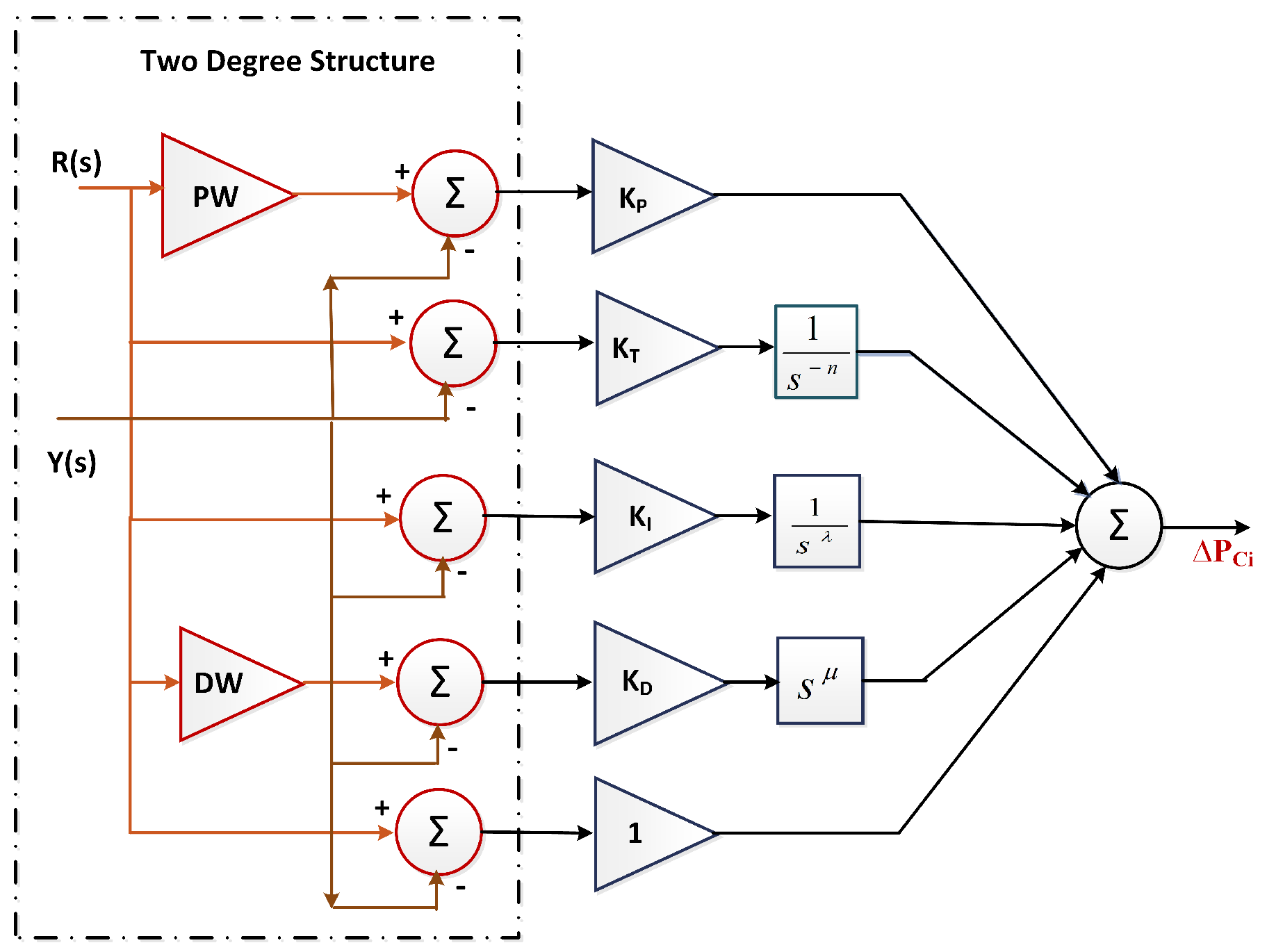
The two-degree-of-freedom fractional-order proportional tilt integral derivative plus one (2DOF-FOPTID+1) controller is designed to address the challenges of modern power systems by combining fractional-order dynamics with a two-degree-of-freedom structure. The detailed structure of the proposed controller is shown in Figure 2. Its architecture consists of five components: they are a proportional term ($K_P$) for immediate response, a tilt term ($K_T/s^n$) for low-frequency disturbance suppression, a fractional-order integral term ($K_I/s^{\lambda }$) for zero steady-state error, a fractional-order derivative term ($K_D{s}^{\mu }$) for improved transient response, and a unity gain (+1) for additional control flexibility, where n, $\lambda$, and $\mu$ are fractional orders. This formulation offers precise tuning capabilities over a broad range of parameter values, making the controller more robust and adaptive than traditional integer-order controllers. Its fractional-order terms ensure finer control over phases and gain margins, while the tilt term enhances stability margins and disturbance rejection, particularly in systems with high variability, such as microgrid-integrated power systems.

In the two-area microgrid-integrated system, the proposed controller optimizes performance by minimizing the area control error (ACE), which is the sum of frequency deviation and tie-line power flow deviation for each area. The controller’s two-degree-of-freedom structure enables independent tuning for setpoint tracking and disturbance rejection, ensuring effective mitigation of load fluctuations and renewable energy intermittency. The fractional-order integral and derivative terms enhance robustness to system nonlinearities, while the tilt term provides superior suppression of low-frequency disturbances. Overall, the proposed controller ensures improved stability, faster dynamic response, and optimal operation of the interconnected two-area system.

3.1. Fractional Calculus of the Proposed Controller

Fractional-order calculus extends traditional calculus by introducing non-integer powers of the Laplace variable s. This generalization transforms the derivative ${\displaystyle \frac{d^{n}y\left(t\right)}{d{t}^n}}$, where n is an integer, into ${\displaystyle \frac{d^{a}y\left(t\right)}{d{t}^a}}$, where a is a non-integer. The Riemann–Liouville (RL) [45] definition is commonly used to describe fractional-order derivatives and is expressed as:

$$a{D}_t^{a}f\left(t\right)={\displaystyle \frac{1}{\mathrm{\Gamma }(n-a)}}{\displaystyle \frac{d^n}{d{t}^n}}{\int }_0^{t}f\left(s\right){(t-s)}^{a-n-1}ds$$

(15)

where $n-1<a<n$, $n\in \mathbb{N}$, and $\mathrm{\Gamma }\left(s\right)$ is the gamma function defined as:

$$\mathrm{\Gamma }\left(s\right)={\int }_0^{\infty }{t}^{s-1}{e}^{-t}dt$$

(16)

Fractional-order dynamics offer improved flexibility and precision for controller design. However, fractional-order terms such as $s^a$ or ${\displaystyle \frac{1}{s^a}}$ must be approximated for practical implementation. This is achieved using the Oustaloup filter (CRONE approximation) [46], which represents the fractional-order element $s^a$ as an integer-order transfer function over a specified frequency range $[{\omega }_L,{\omega }_H]$. The approximation is expressed as

$$s^a\approx K{\displaystyle \prod _{k=-N}^N}{\displaystyle \frac{s+{\omega }_{z_k}}{s+{\omega }_{p_k}}}$$

(17)

where:

$$K={\omega }_H^a,{\omega }_{z_k}={\omega }_L{\left({\displaystyle \frac{{\omega }_H}{{\omega }_L}}\right)}^{{\displaystyle \frac{k+N+0.5(1-a)}{2N+1}}},{\omega }_{p_k}={\omega }_L{\left({\displaystyle \frac{{\omega }_H}{{\omega }_L}}\right)}^{{\displaystyle \frac{k+N+0.5(1+a)}{2N+1}}}$$

(18)

For this study, the Oustaloup approximation is applied with $N=3$ and a frequency range of $[{10}^{-2},{10}^2]$ rad/s, providing a balance between precision and computational complexity.

3.2. Controller Designing

The 2DOF-FOPTID+1 controller takes the reference input $R\left(s\right)$ and feedback signal $Y\left(s\right)$, scaled by the proportional weight $PW$ and disturbance weight $DW$, respectively. These inputs generate error signals processed through proportional, integral, derivative, first-order, and constant components. Fractional-order terms ${\displaystyle \frac{1}{s^{\lambda }}}$, $s^{\mu }$, and ${\displaystyle \frac{1}{s^n}}$ are approximated using the Oustaloup filter. The proportional weight enhances reference tracking, while the disturbance weight reduces external disturbances. The controller output, represented as $\mathrm{\Delta }{P}_c\left(s\right)$, is determined by the combination of various control terms acting on the error signals. The expression for the controller output is given as follows:

$$\mathrm{\Delta }{P}_c\left(s\right)=\left[K_P+{\displaystyle \frac{K_I}{s^{\lambda }}}+K_D{s}^{\mu }+{\displaystyle \frac{K_T}{s^n}}+1\right]·(R\left(s\right)·PW-Y\left(s\right)·DW)$$

(19)

The corresponding transfer function of the controller is represented as follows:

$$GC\left(s\right)=\left[K_P+{\displaystyle \frac{K_I}{s^{\lambda }}}+K_D{s}^{\mu }+{\displaystyle \frac{K_T}{s^n}}+1\right]·PW-\left[K_P+{\displaystyle \frac{K_I}{s^{\lambda }}}+K_D{s}^{\mu }+{\displaystyle \frac{K_T}{s^n}}+1\right]·DW$$

(20)

The Oustaloup approximation combined with the two-degree-of-freedom structure allows the controller to balance accurate reference tracking and effective disturbance rejection. The reference controller, $K_{Ref}\left(s\right)$, is designed to ensure the closed-loop response follows a specified reference model.

$$G_{ref}\left(s\right)={\displaystyle \frac{{\omega }_{ref}^2}{s^2+2\xi {\omega }_{ref}s+{\omega }_{ref}^2}}$$

(21)

Here, ${\omega }_{ref}$ is the natural frequency set to 1000 rad/s, and $\xi$ is the damping coefficient set to 0.707. These parameters ensure a fast transient response with minimal overshoot, enhancing the system’s ability to follow the desired trajectory. To minimize external disturbances, the disturbance weight $DW\left(s\right)$ is designed to satisfy the following condition:

$$1-GP\left(s\right)·DW\left(s\right)\approx 0$$

(22)

In this context, $GP\left(s\right)$ refers to the plant transfer function. While perfect disturbance cancellation may not always be achievable, optimal tuning of $DW\left(s\right)$ significantly mitigates disturbances, ensuring robust performance under varying conditions. The effectiveness of the 2DOF-FOPTID+1 controller depends on selecting appropriate parameters, including proportional, integral, derivative, and first-order gains ($K_P$, $K_I$, $K_D$, $K_T$), fractional orders ($\lambda$, $\mu$, n), and weights ($PW$, $DW$). These parameters are chosen within the following ranges:

$$K_P,K_I,K_D,K_T\in [0,5],\lambda ,\mu ,n\in [0,1.5],PW,DW\in [0,1]$$

(23)

The Oustaloup approximation parameters are tuned to represent fractional-order terms accurately, while MWA optimally adjusts the controller parameters, ensuring precise reference tracking, effective disturbance rejection, and stable transients. Details are provided in Algorithm 1.    

Algorithm 1: Modified Walrus Optimization Algorithm (MWA)

3.3. Theoretical Justification of the Proposed Controller

The proposed controller is designed to solve real problems in a two-area microgrid system. In interconnected networks, a sudden power change in one area quickly affects the frequency and power flow in the other area. Basic controllers struggle with interconnected changes because making them fast at reaching the target frequency makes them weak against sudden power shifts. The two-degree-of-freedom structure solves the problem by using two different paths. One path works only to keep the frequency and tie-line power flow exactly on target. The other path works only to handle sudden power disturbances from either area. The separation of tasks allows the microgrids to stay safe and stable during unexpected power changes without going past normal limits.

To make the overall system even more reliable, fractional mathematics are used to fix the rigid nature of standard controllers. Fractional control adds a special stability that keeps the entire two-area system balanced even if grid conditions or power generation change suddenly. In addition to the added stability, a tilt component is included to handle the slow frequency drops that occur when the power demand changes between the two areas. The tilt part pushes back hard against slow power drops and brings the microgrids back to normal operation much faster than standard controllers can achieve.

Finally, the “+1” structure is added as a low-pass filter to handle high-frequency noise and measurement errors present in any power network. Without a filter, controllers react to every small fluctuation and send rapid, aggressive signals to the generators, which can physically damage the machines over time. The filter blocks unnecessary noise, so the controller only responds to actual power changes. Due to the filtering action, the proposed method performs much better than existing state-of-the-art controllers even in standard scenarios without electric vehicles. When electric vehicles are integrated, the filter becomes even more valuable by successfully blocking fast, chaotic signals caused by constant charging and discharging. By assembling all parts, the proposed controller offers fast responses, strong stability, and safe operation for the whole two-area system under various conditions.

3.4. Optimization of Controller Parameters

A metaheuristic optimization algorithm is an iterative process that guides a subordinate heuristic by intelligently combining different concepts for exploring and exploiting the search space [47,48]. Learning strategies are used to identify an efficient and optimal solution [49,50]. The modified walrus optimization algorithm extends the traditional approach [51] by incorporating opposition-based learning [52] to enhance exploration and exploitation in two-area LFC problems. MWA evaluates candidate solutions and their opposites simultaneously, improving convergence to the global optimum. It applies opposition-based learning during both initialization and updates to ensure diverse and high-quality solutions. The fitness of each solution is determined using a modified ITAE objective function that accounts for frequency and tie-line power deviations.

$$\mathrm{ITAE}={\int }_0^{T}t·\left(|\mathrm{\Delta }{f}_1\left(t\right)|+|\mathrm{\Delta }{f}_2\left(t\right)|+|\mathrm{\Delta }{P}_{\mathrm{tie}}\left(t\right)|\right)dt$$

(24)

where $\mathrm{\Delta }{f}_1\left(t\right)$ and $\mathrm{\Delta }{f}_2\left(t\right)$ represent frequency deviations in Area 1 and Area 2, respectively, while $\mathrm{\Delta }{P}_{\mathrm{tie}}\left(t\right)$ denotes the tie-line power deviation over the simulation time T. In the iterative update phase, opposition-based learning enhances solution refinement by applying it to all three optimization phases: feeding, migration, and escaping. This strategy ensures efficient exploration while maintaining solution diversity, leading to improved optimization performance.

To ensure a fair comparison and reproducibility, the parameter settings for all evaluated optimization algorithms are established uniformly. For the proposed MWA, the population size (N) is set to 50, and the maximum number of iterations is limited to 50. A population size of 50 provides an optimal balance, ensuring diverse exploration of the complex controller parameter space without causing excessive computational overhead.

Beyond convergence accuracy, evaluating the computational complexity is essential for practical engineering implementation. The theoretical computational complexity of the proposed MWA depends primarily on the population size (N), the number of controller parameters or dimensions (D), and the maximum number of iterations (MaxIter). During the initialization phase, generating the random population, computing the opposite positions, and evaluating the initial fitness requires a time complexity of $\mathcal{O}(N\times D)$. Within the main iterative loop, updating the positions and evaluating the fitness across the feeding, migration, and escaping phases yields a complexity of $\mathcal{O}(\mathrm{MaxIter}\times N\times D)$. Therefore, the overall theoretical computational complexity is expressed as:

$$\mathcal{O}\left(\mathrm{MWA}\right)=\mathcal{O}(N\times D+\mathrm{MaxIter}\times N\times D)\approx \mathcal{O}(\mathrm{MaxIter}\times N\times D)$$

(25)

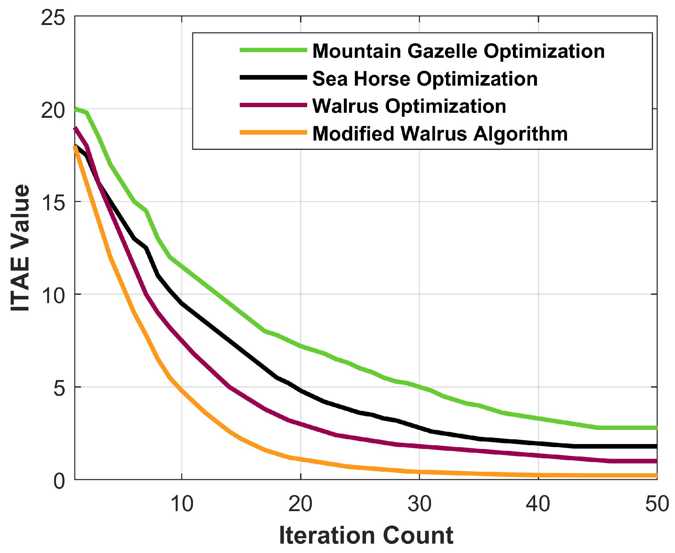
Because MWA does not introduce highly complex inner loops compared to standard heuristic algorithms, it achieves superior convergence capabilities without a significant increase in theoretical execution time. MWA combines the strengths of opposition-based learning and the adaptive behaviors of walruses, ensuring robust performance in two-area LFC problems. By minimizing frequency and tie-line power deviations using the modified ITAE, the algorithm guarantees optimal control parameter tuning, faster convergence, and improved stability in complex power systems. Further, the performance of this optimization technique is compared with other recent optimizations like sea-horse optimization [53] and Mountain Gazelle Optimizer [54], which are proven better than the traditional particle swarm optimization [55]. The respective convergence plots relevant to the considered system with EV integration are shown in Figure 3. Compared to the other techniques, the considered technique yields the lowest ITAE value.

To further validate the robustness of the proposed algorithm and rule out the influence of randomness, a statistical analysis based on 10 independent runs was conducted. The mean performance, standard deviation, and average computational execution time are summarized in

Table 2. Statistical performance analysis of different algorithms over 10 independent runs.

Algorithm	Best Fitness	Mean Fitness	Std. Deviation	Avg. Time (min)
MWA (Proposed)	0.7220	0.7254	0.0018	56.45
WAO	0.7541	0.7612	0.0042	74.12
SHO	0.8125	0.8256	0.0115	91.54
MGO	0.8763	0.8921	0.0234	104.82

. The results demonstrate that MWA consistently achieves the lowest mean fitness with minimal deviation, confirming its superior reliability and efficiency.

3.5. Eigen Value Analysis

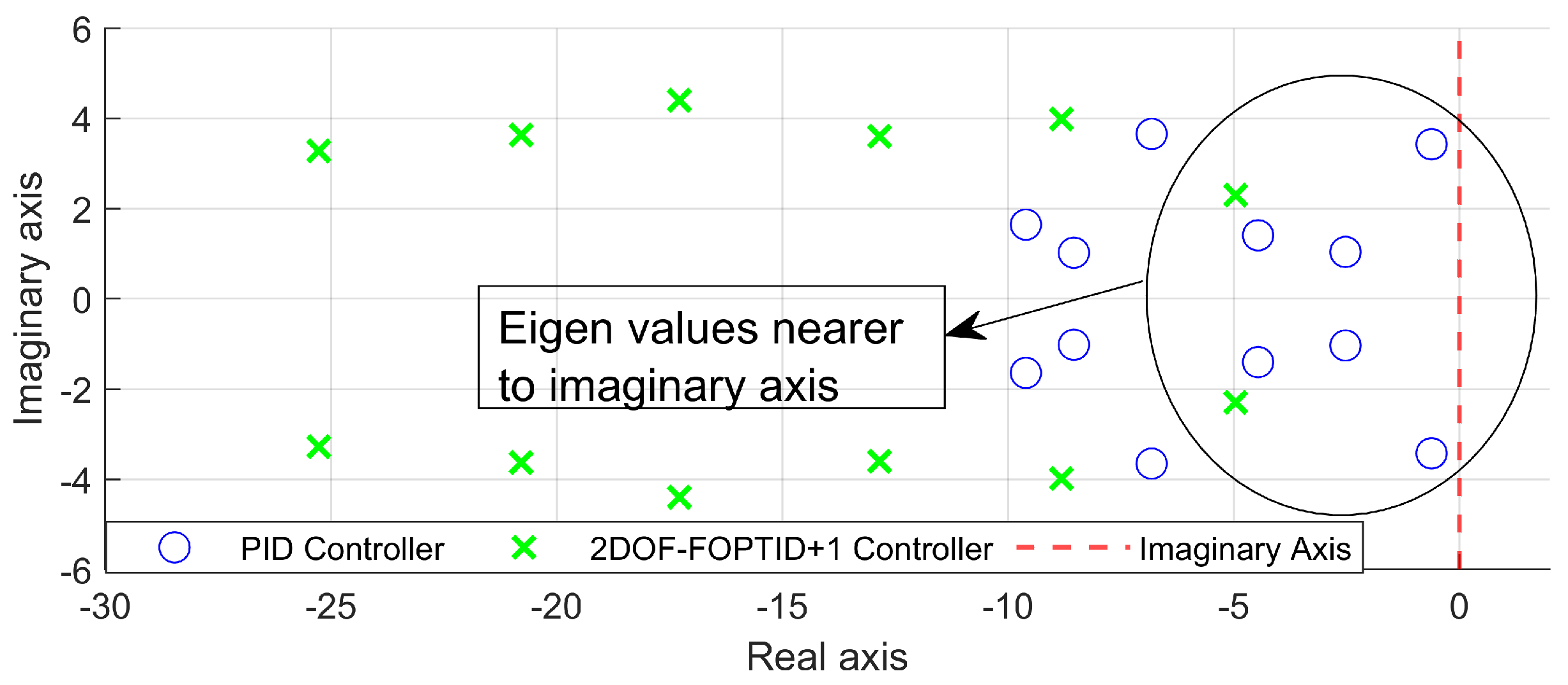
The state-space analysis performed on the system facilitates the evaluation of its dynamic behavior through eigenvalue computation. The eigenvalues obtained under the application of both the conventional PID controller and the proposed 2DOF-FOPTID+1 controller are presented in

Table 3. Eigenvalues.

Eigenvalues with PID	$-0.6129\pm 3.4257\mathit{i}$; $-2.5201\pm 1.0368\mathit{i}$; $-4.4580\pm 1.4059\mathit{i}$; $-6.8159\pm 3.6540\mathit{i}$; $-8.5384\pm 1.0202\mathit{i}$; $-9.6014\pm 1.6432\mathit{i}$
Eigenvalues with Proposed Controller	$-4.9513\pm 2.3016i$; $-8.8081\pm 3.9860i$; $-12.8480\pm 3.5985i$; $-17.2757\pm 4.3969i$; $-20.7878\pm 3.6305i$; $-25.2628\pm 3.2732i$

and visualized in the s-plane in Figure 4. It is evident that, for the PID controller, most eigenvalues lie close to the imaginary axis. These dominant poles significantly influence the system response, leading to slower dynamics and potential stability challenges. In contrast, the eigenvalues corresponding to the proposed controller are positioned farther to the left in the s-plane. This leftward shift is attributed to the two-degree-of-freedom structure and the fractional-order components of the proposed controller, which effectively suppress the influence of dominant poles and enhance system stability by accelerating the transient response.

4. Results and Discussions

To investigate the efficacy and robustness of the proposed controller, a two-area MIP is considered in this study. The performance of the proposed controller is evaluated and compared with that of existing benchmark controllers. Additionally, the controller is tested in conjunction with an AEV model under various operating scenarios, including step load changes, random load disturbances, and random solar generation input. Real-time validation is performed for the random load case using the OPAL-RT platform, ensuring practical feasibility. To assess robustness, key system parameters such as time constants and gains are varied, and the controller’s response is analyzed. The results of these investigations are presented in the following subsections.

4.1. Scenario-I: Performance Analysis of Proposed Controller with the Existing Controllers

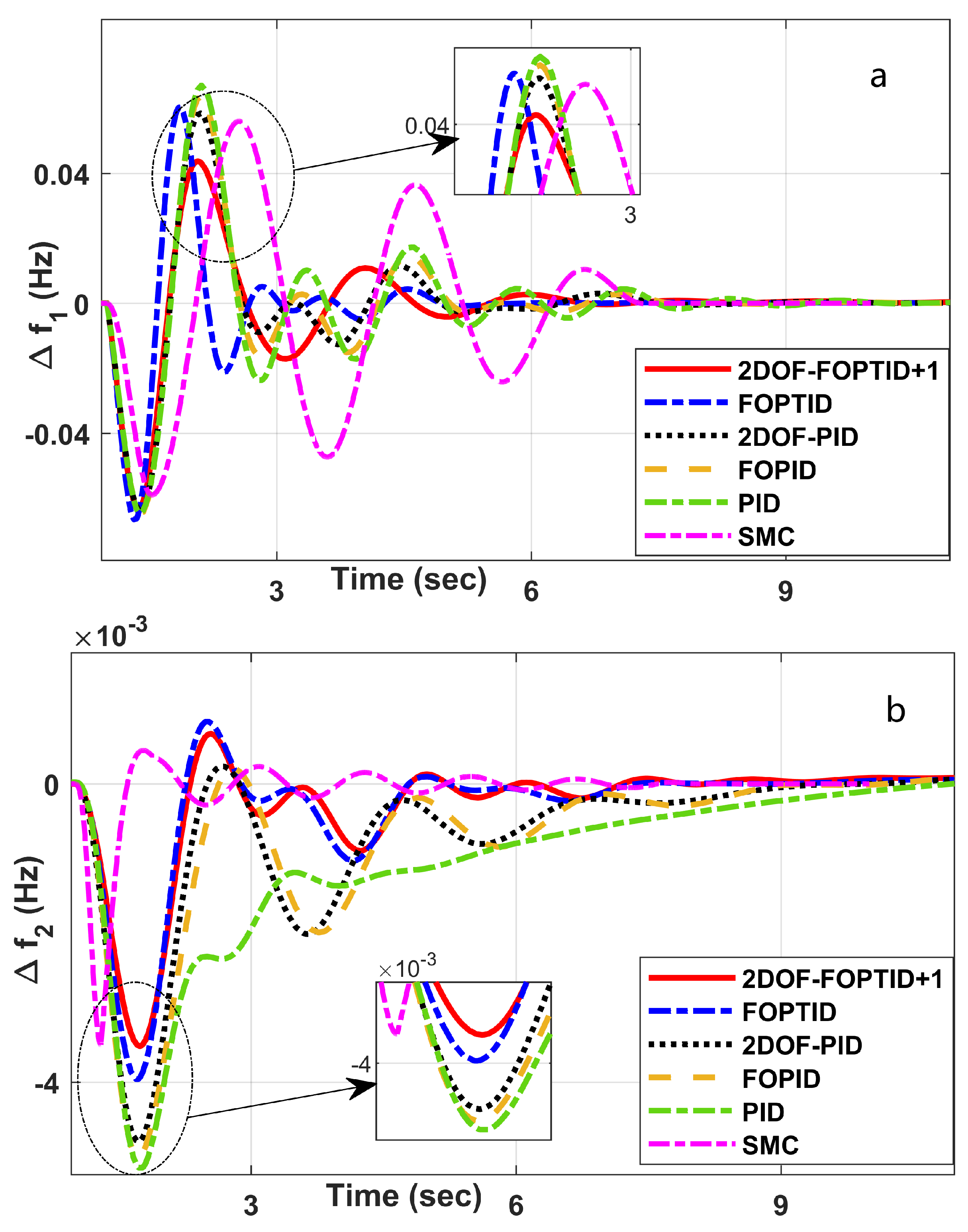
This section evaluates the dynamic behavior of the two-area LFC system by introducing the proposed controller in both areas. The responses obtained against the traditional controllers, like PID [7], FOPID [8], 2DOF-PID [10], FOPTID [42] and sliding mode controller(SMC) [25] controllers are investigated. The controller parameters optimized using the MWA technique are summarized in

Table 4. Controller parameters tuned using MWA: without EV.

Controller	Area	${\mathit{K}}_{\mathit{P}}$	${\mathit{K}}_{\mathit{T}}$	${\mathit{K}}_{\mathit{I}}$	${\mathit{K}}_{\mathit{D}}$	n	$\mathit{\lambda }$	$\mathit{\mu }$	PW	DW
PID	Area-1	2.034	-	4.591	1.697	-	-	-	-	-
	Area-2	2.084	-	3.970	0.824	-	-	-	-	-
FOPID	Area-1	3.887	-	4.069	1.589	-	0.487	0.435	-	-
	Area-2	1.744	-	4.126	2.033	-	0.482	0.741	-	-
2DOF-PID	Area-1	2.241	-	3.618	1.342	-	-	-	0.854	1.123
	Area-2	3.476	-	1.637	3.473	-	-	-	1.052	0.941
FOPTID	Area-1	4.786	2.447	3.929	1.522	0.491	0.837	0.537	-	-
	Area-2	3.046	2.822	4.651	2.602	0.298	0.711	0.818	-	-
2DOF-FOPTID+1	Area-1	3.207	1.026	2.917	1.330	0.505	0.687	0.616	0.765	1.204
	Area-2	1.957	2.052	2.249	0.609	0.932	0.521	0.408	0.988	0.876

, while the SMC tuned via MWA yields the optimal values ${\rho }_{i1}=7.82$, ${\rho }_{i2}=0.64$, ${\rho }_{i3}=0.27,{\rho }_{i4}=3.41,{\rho }_{i5}=12.88,k_i=11.67, {\eta }_i=5.13$. The frequency responses attained are depicted in Figure 5. The time domain specifications of the responses using the various listed controllers are produced in

Table 5. Comparison of time domain specifications and ITAE values with various controllers for scenario-I.

Controller	Area 1 Frequency Deviation				Area 2 Frequency Deviation				ITAE
	OS	US	ST (s)	P2P	OS	US	ST (s)	P2P
PID	0.067	0.065	10.16	0.1316	0	$5.1\times {10}^{-3}$	10.48	0.00514	2.766
FOPID	0.064	0.064	9.12	0.1280	0	$5\times {10}^{-3}$	9.17	0.00500	1.921
2DOF-PID	0.058	0.064	8.91	0.1224	$2.3\times {10}^{-4}$	$4.8\times {10}^{-3}$	9.82	0.00502	1.884
FOPTID	0.060	0.066	7.42	0.1266	$1.0\times {10}^{-3}$	$3.8\times {10}^{-3}$	8.13	0.00483	1.827
SMC	0.056	0.058	8.09	0.1140	$4.4\times {10}^{-4}$	$3.4\times {10}^{-3}$	8.14	0.00384	0.745
2DOF-FOPTID+1	0.044	0.063	6.17	0.1068	$8\times {10}^{-4}$	$4\times {10}^{-3}$	7.54	0.00476	0.722

. The peak-to-peak (P2P) value, a metric that relies on overshoot (OS) and undershoot (US), serves as a valuable tool for comparing the magnitude of frequency deviations. In Area 1, the 2DOF-FOPTID+1 controller demonstrates a minimal P2P value of 0.1068 Hz, achieving percentage reductions of 18.85%, 16.56%, 12.75%, 15.64% and 6.32% when compared to the PID, FOPID, 2DOF-PID, FOPTID and SMC controllers, respectively.

Additionally, the proposed controller stabilizes the frequency deviations within 6.17 s, resulting in percentage reductions of 39.27%, 32.35%, 30.75%, 16.85%, 23.72% compared to the same controllers.

Similarly, in Area 2, the proposed controller outperforms the other controllers. The peak-to-peak value reductions are 7.39%, 4.80%, 5.18%, 1.45% and 2.17% when compared to the PID, FOPID, 2DOF-PID, FOPTID and SMC controllers, respectively. While the reduction in peak-to-peak deviations is moderate, a significant improvement is observed in settling time (ST), with reductions of 28.05%, 17.78%, 23.22%, 7.26%, 6.37% over the same controllers. Hence, the proposed controller derives the optimal frequency responses when compared with the traditional controllers; even the objective value, i.e., ITAE, achieved with the optimal parameters of the proposed controller is lowest when compared with the existing controllers, demonstrating its effectiveness in improving system stability.

4.2. Scenario-II: Performance of the Considered System After Integration of AEV

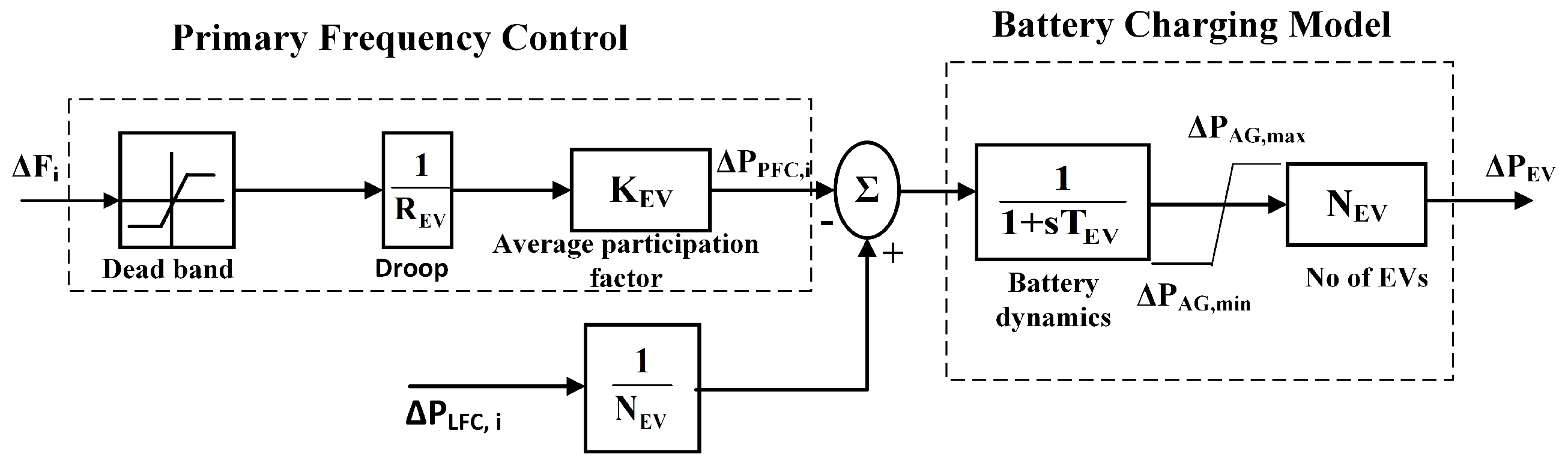
In this scenario, an aggregated electric vehicle [56] shown in Figure 6 is integrated in Area 2, which helps to overcome the intermittency of renewable units and provides a reliable power supply, thereby lessening the frequency fluctuations in the system. The AEV parameters in

Table 6. Parameters of the Aggregated Electric Vehicle (AEV) Model [57].

Parameter	Symbol	Value
Time constant	$T_{EV}$	0.1 s
Maximum/Minimum SOC	$SO{C}_{max}/SO{C}_{min}$	0.9/0.1
Max Charging/Discharging Power	$\mathrm{\Delta }{P}_{EV}^{max}/\mathrm{\Delta }{P}_{EV}^{min}$	$\pm 10$ kW
Inverter Gain	$K_{EV}$	1.0

are based on the aggregated model of a standard passenger EV fleet reported in [57].

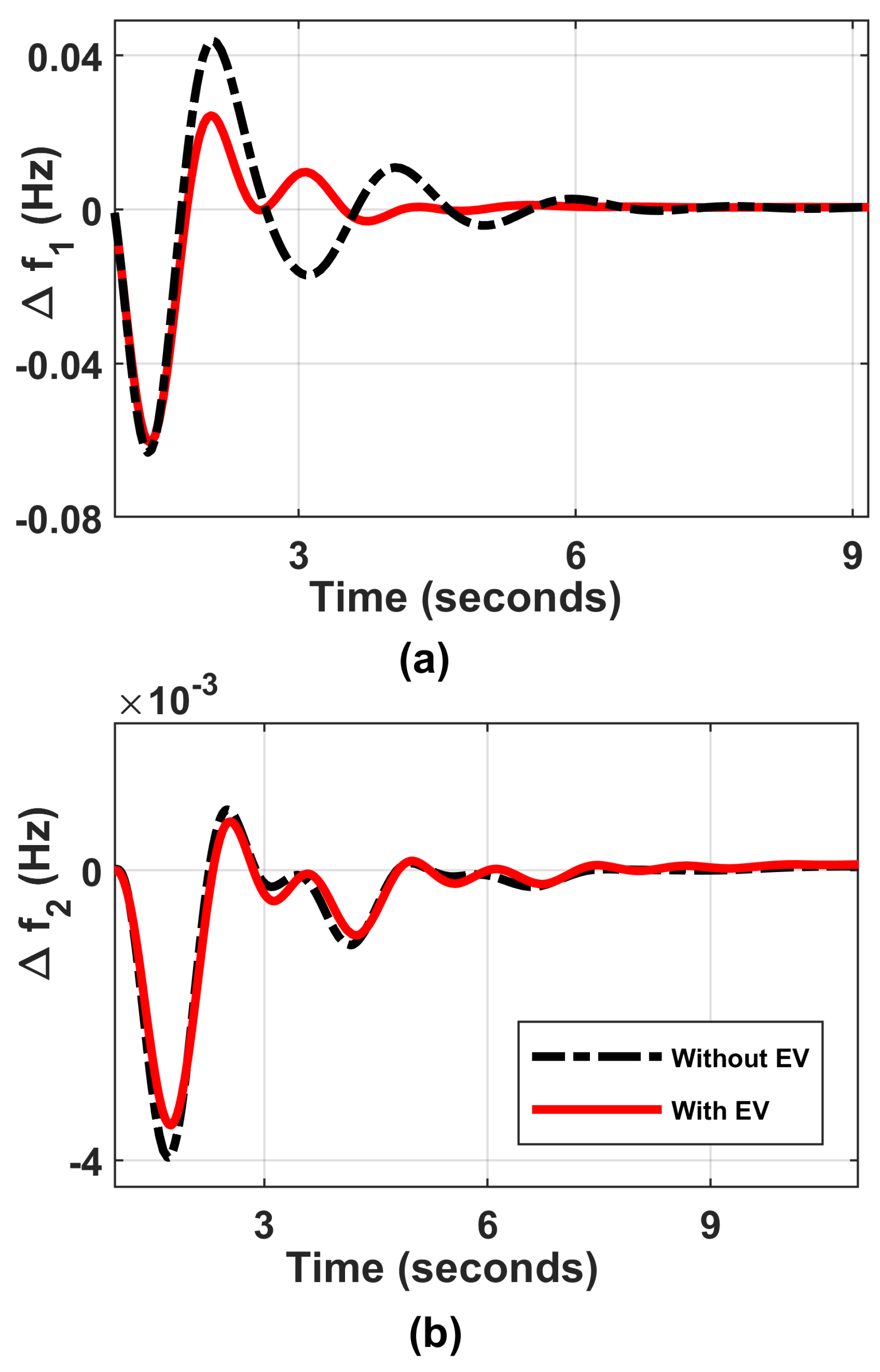
This section compares the performance of the system after integration of AEVs into the microgrid while the proposed controller is deployed in both areas, where the optimal parameters are taken from scenario 1. The comparison of the frequency responses after placement of AEVs into the system is provided in Figure 7, which illustrates the frequency deviations for both areas under the proposed controller, comparing cases with and without AEV integration.

From

Table 7. Comparison of time domain specifications after integration of AEV.

Controller	Area 1 Frequency Deviation				Area 2 Frequency Deviation
	OS	US	ST (s)	P2P	OS	US	ST (s)	P2P
Without AEV	0.044	0.063	6.17	0.1068	$8\times {10}^{-4}$	$4\times {10}^{-3}$	7.54	0.00476
With AEV (100% fleet)	0.024	0.061	4.89	0.0845	0	0.0035	7.32	0.00351
With AEV (50% fleet)	0.037	0.061	5.82	0.098	$2\times {10}^{-4}$	$4\times {10}^{-3}$	7.41	0.0042
With AEV (30% fleet)	0.041	0.063	6.11	0.104	$7\times {10}^{-4}$	$4\times {10}^{-3}$	7.49	0.0047

, it is identified that the inclusion of AEVs reduces the peak-to-peak frequency deviation from 0.1068 Hz to 0.0845 Hz, achieving a 20.88% reduction. Additionally, the settling time improves by 20.75%, decreasing from 6.17 s to 4.89 s in Area 1 frequency responses, demonstrating the effectiveness of AEVs in stabilizing frequency fluctuations.

In Area 2, the proposed controller with AEV integration achieves a 26.26% reduction in peak-to-peak deviation, decreasing from 0.00476 Hz to 0.00351 Hz. Although the improvement in settling time is relatively smaller at 2.92% (from 7.54 s to 7.32 s), the presence of AEVs contributes significantly to reducing frequency deviations and enhancing overall system stability. These results emphasize the importance of AEV integration in improving system performance. The reduction in transients and enhanced frequency response demonstrate that incorporating AEVs into the system with the proposed controller leads to greater efficiency and stability. These findings reinforce the role of AEV-based frequency support in modern power systems.

4.3. Scenario-III: Robustness Analysis

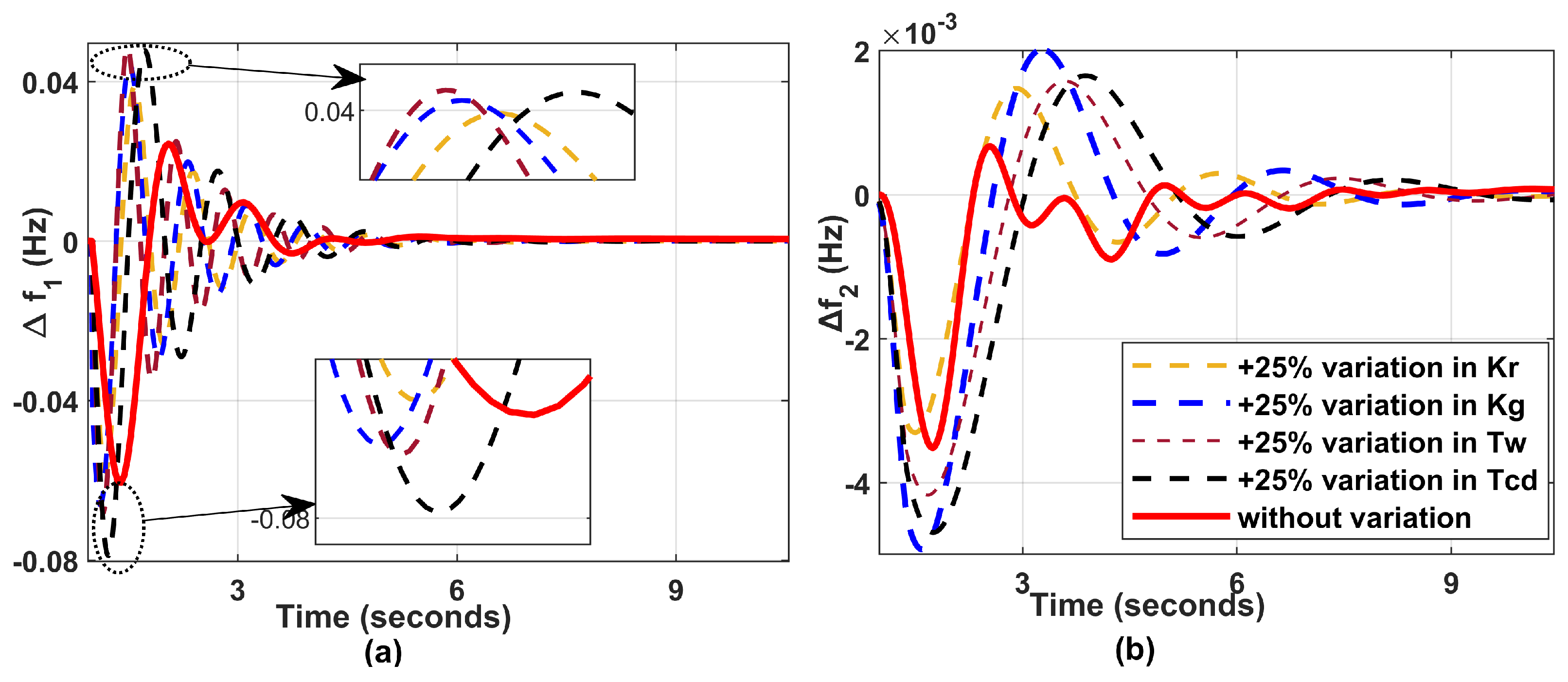
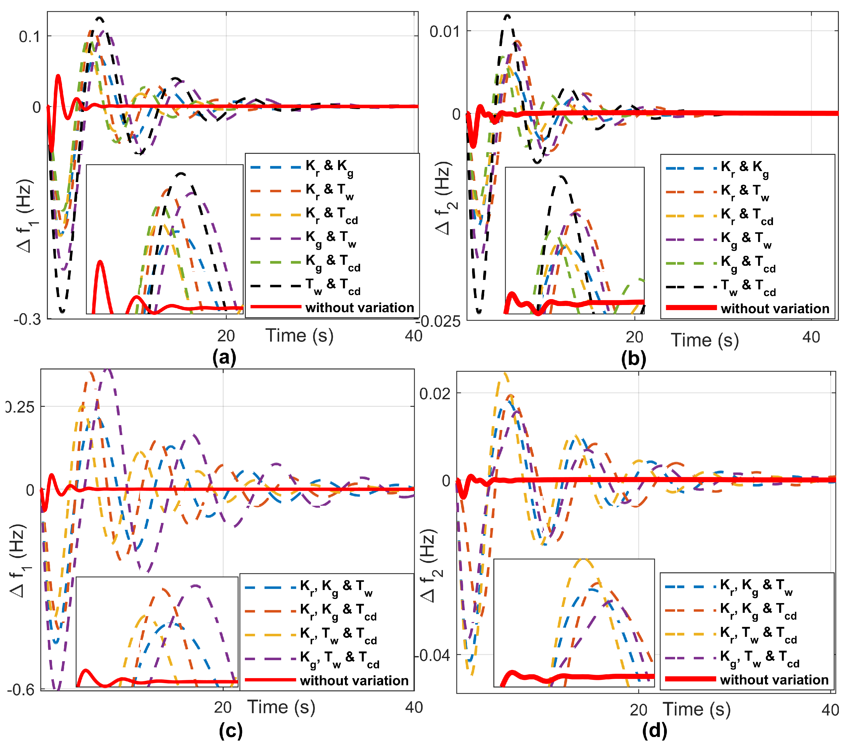
The robustness of the proposed controller is evaluated by analyzing the system’s response to variations in the parameters $K_r$, $K_g$, $T_w$, and $T_{cd}$. Each parameter is individually increased by 25% of its nominal value in the system, including the AEV component. The corresponding system responses are illustrated in Figure 8.

The analysis reveals that these parameter variations lead to amplified transients in frequency deviations, with the most significant impact observed in settling times. Despite the worsened frequency deviations, the proposed controller successfully regulates the system within stability limits. The P2P and ST values corresponding to these single-parameter variations are presented in

Table 8. Variation in time domain specifications with parameter variation.

Area	Time	${\mathit{K}}_{\mathit{r}}$		${\mathit{K}}_{\mathit{g}}$		${\mathit{T}}_{\mathit{w}}$		${\mathit{T}}_{\mathbf{cd}}$
	Domain	Value	% Inc.	Value	% Inc.	Value	% Inc.	Value	% Inc.
$\mathrm{\Delta }{f}_1$	P2P (Hz)	0.095	11.76	0.11	29.41	0.12	41.18	0.13	52.94
	ST (s)	8.47	16.99	8.62	19.06	8.96	23.76	8.39	15.89
$\mathrm{\Delta }{f}_2$	P2P (Hz)	0.0048	6.67	0.0069	53.33	0.0058	28.89	0.0064	42.22
	ST (s)	9.22	16.56	9.04	14.29	10.11	27.81	9.49	19.98

% Inc.: Percentage Increase.

. The results indicate that settling times increase by a maximum of 23.76% in Area 1 and 27.81% in Area 2. Additionally, in only two instances, the P2P variations exceed 50%, while in all other cases, deviations remain within nominal limits.

To further validate the controller’s resilience, the system was subjected to simultaneous multiple parameter variations, as depicted in Figure 9. Figure 9a,b illustrate the frequency deviations when two system parameters are varied concurrently, while Figure 9c,d present the responses under three simultaneous parameter variations. As expected, these severe multi-parameter deviations lead to an observable degradation in performance, resulting in higher overshoots and longer settling times compared to single-parameter changes. However, even under these extreme parametric uncertainties, the proposed controller ensures that the system regains a stable steady-state. Crucially, the maximum frequency deviations remain strictly within the permissible tolerance limits of $\pm 0.5$ Hz.

Overall, the proposed controller effectively mitigates instability, keeping the system near its optimal operating state despite severe single and multi-parameter variations. These findings highlight the robustness of the controller, ensuring reliable and acceptable performance even under highly dynamic and uncertain system conditions.

4.4. Scenario-IV: Dynamic Study with Random Input and Random Load Disturbance

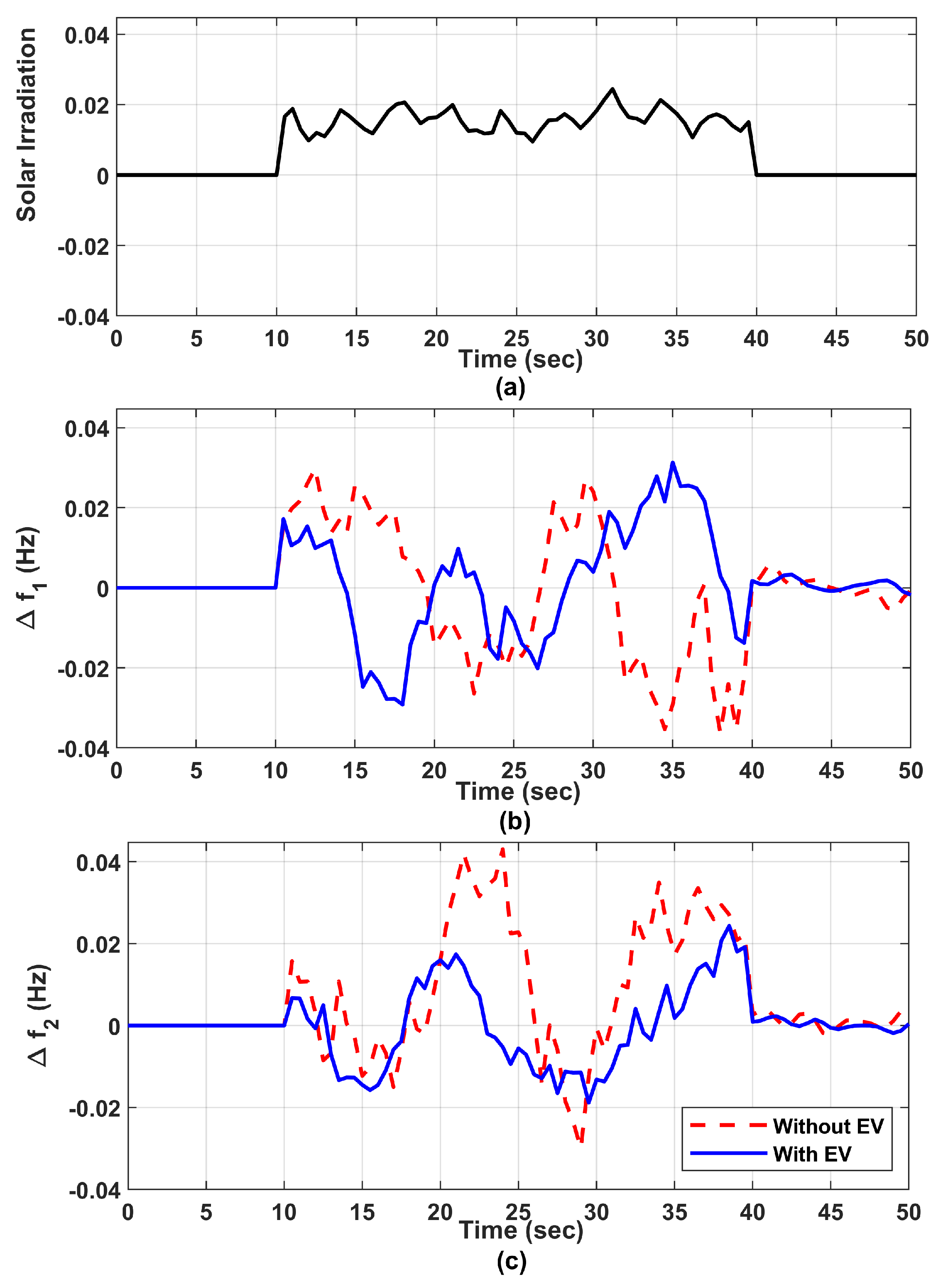
This study examines the impact of random solar irradiance and random load disturbances on system frequency regulation. The objective is to analyze how the proposed controller, optimized using MWA, maintains system stability under varying conditions. As shown in Figure 10a, a random solar irradiance signal is applied to the solar unit while keeping the load disturbance at zero. The input remains zero for the first 10 s, followed by a random signal introduced between 10 and 40 s, after which the solar input is set to zero. The resulting frequency responses indicate no deviations up to 10 s, followed by fluctuations in both areas during the 10–40 s interval. Once the solar input ceases after 40 s, frequency deviations gradually stabilize towards zero. The proposed controller effectively maintains frequency deviations within the permissible range of 49.5 Hz to 50.5 Hz, highlighting the significant role of solar power in frequency regulation.

The study is further conducted with and without the integration of AEVs. The presence of AEVs enhances transient response, leading to faster stabilization of frequency deviations when the solar input is held constant. With AEV integration, the statistical metric are reduced predominantly and are produced in

Table 9. Statistics of frequency deviations with random solar input.

Area	Case	Max Dev	Mean Dev	Std Dev	RMSE
$\mathrm{\Delta }{f}_1$	Without AEV	0.047	0.010	0.014	0.015
	With AEV	0.025	0.005	0.007	0.007
$\mathrm{\Delta }{f}_2$	Without AEV	0.033	0.008	0.011	0.012
	With AEV	0.018	0.004	0.006	0.006

. The respective frequency deviations are illustrated in Figure 10b,c.

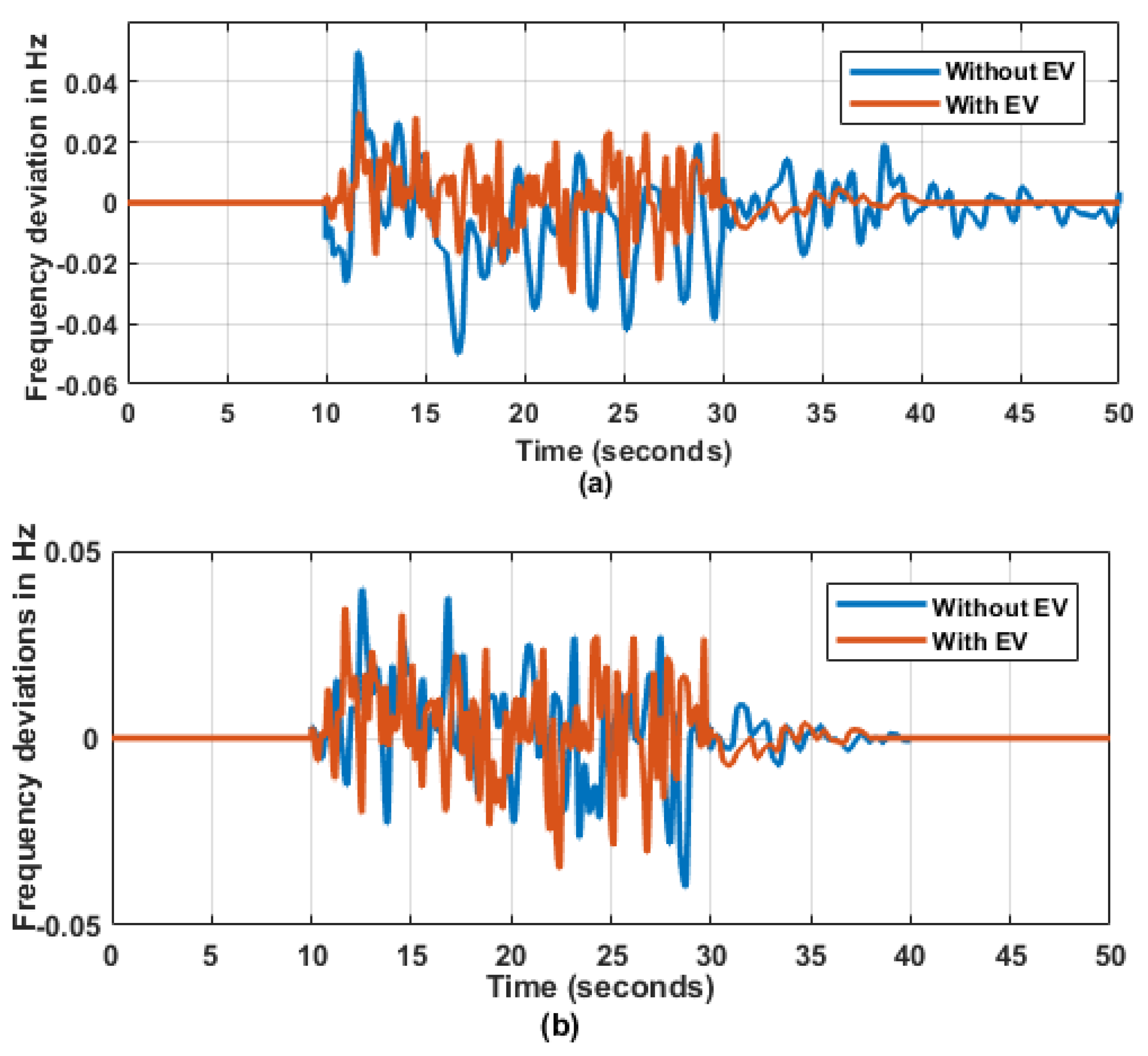
Additionally, an extended analysis is performed by maintaining constant solar irradiation while introducing random load disturbances. A disturbance is applied between 10 and 40 s, leading to observable frequency deviations in both areas. However, the deviations remain within the acceptable limits of 49.5 Hz to 50.5 Hz. The integration of AEVs accelerates system stabilization once the disturbance is removed. The respective frequency responses are shown in Figure 11a for area-1 and Figure 11b for Area 2. Notably, a considerable reduction is observed in maximum deviation (Max Dev), mean deviation, standard deviation (Std Dev), and root mean square error (RMSE), which is made available in

Table 10. Statistics of frequency deviations with random load disturbances.

Area	Case	Max Dev		Min Dev		Mean Dev		Std Dev		RMSE
		Sim	HIL	Sim	HIL	Sim	HIL	Sim	HIL	Sim	HIL
$\mathrm{\Delta }{f}_1$	Without AEV	0.500	0.520	0.005	0.007	0.083	0.089	0.126	0.132	0.131	0.136
	With AEV	0.300	0.315	0.003	0.004	0.039	0.042	0.070	0.074	0.070	0.073
$\mathrm{\Delta }{f}_2$	Without AEV	0.400	0.420	0.004	0.006	0.047	0.050	0.089	0.093	0.089	0.093
	With AEV	0.350	0.365	0.003	0.004	0.044	0.046	0.081	0.085	0.082	0.085

Note. Sim denotes MATLAB/Simulink metrics. HIL denotes real-time hardware-in-the-loop metrics.

, further reinforcing the role of AEVs in enhancing system stability. These findings emphasize the effectiveness of the proposed controller in managing system frequency under dynamic conditions. The results demonstrate that integrating AEVs into the system improves transient response and overall stability, making them a valuable component in modern power systems.

4.5. Scenario-V: Real-Time Validation

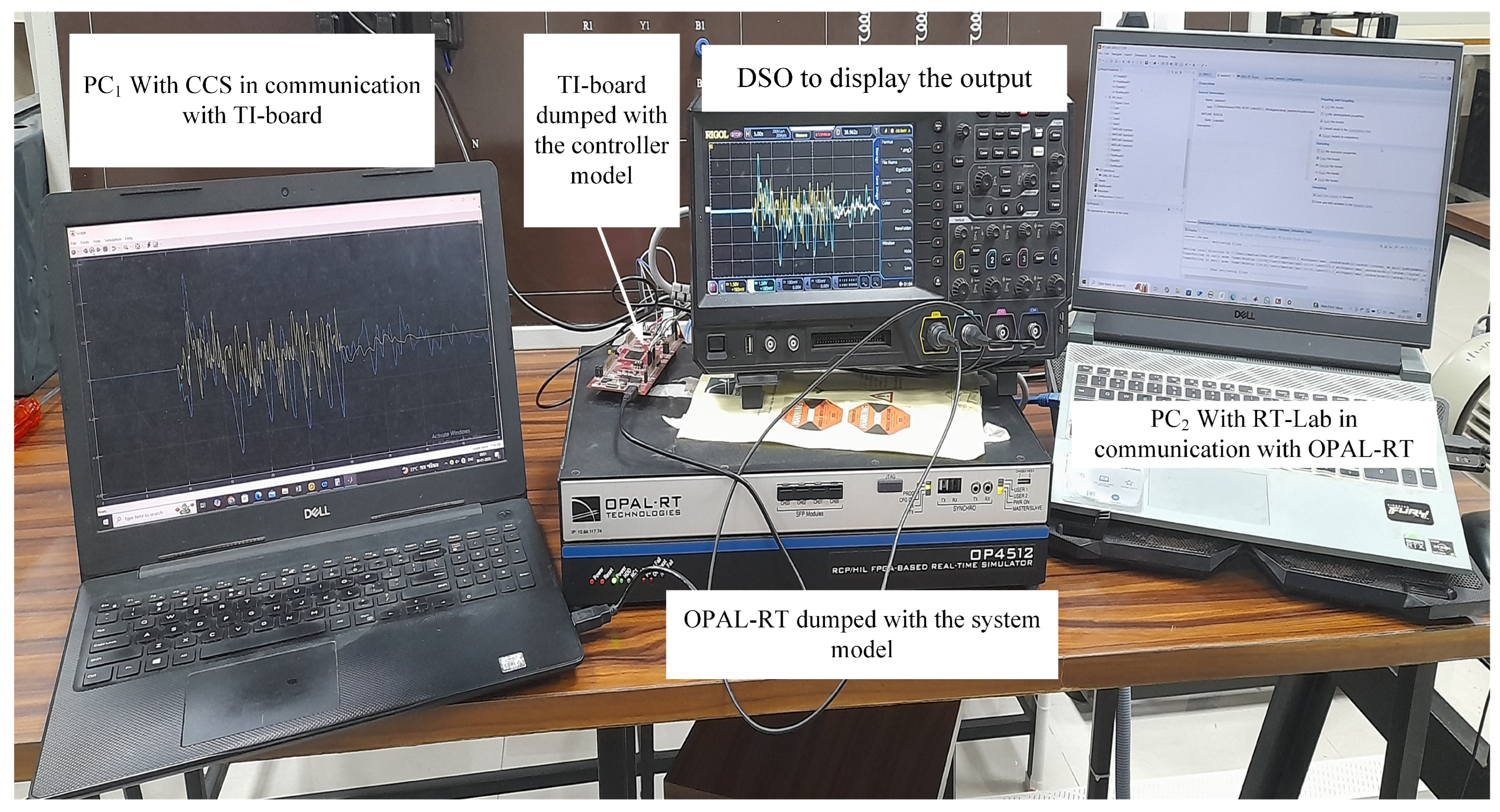
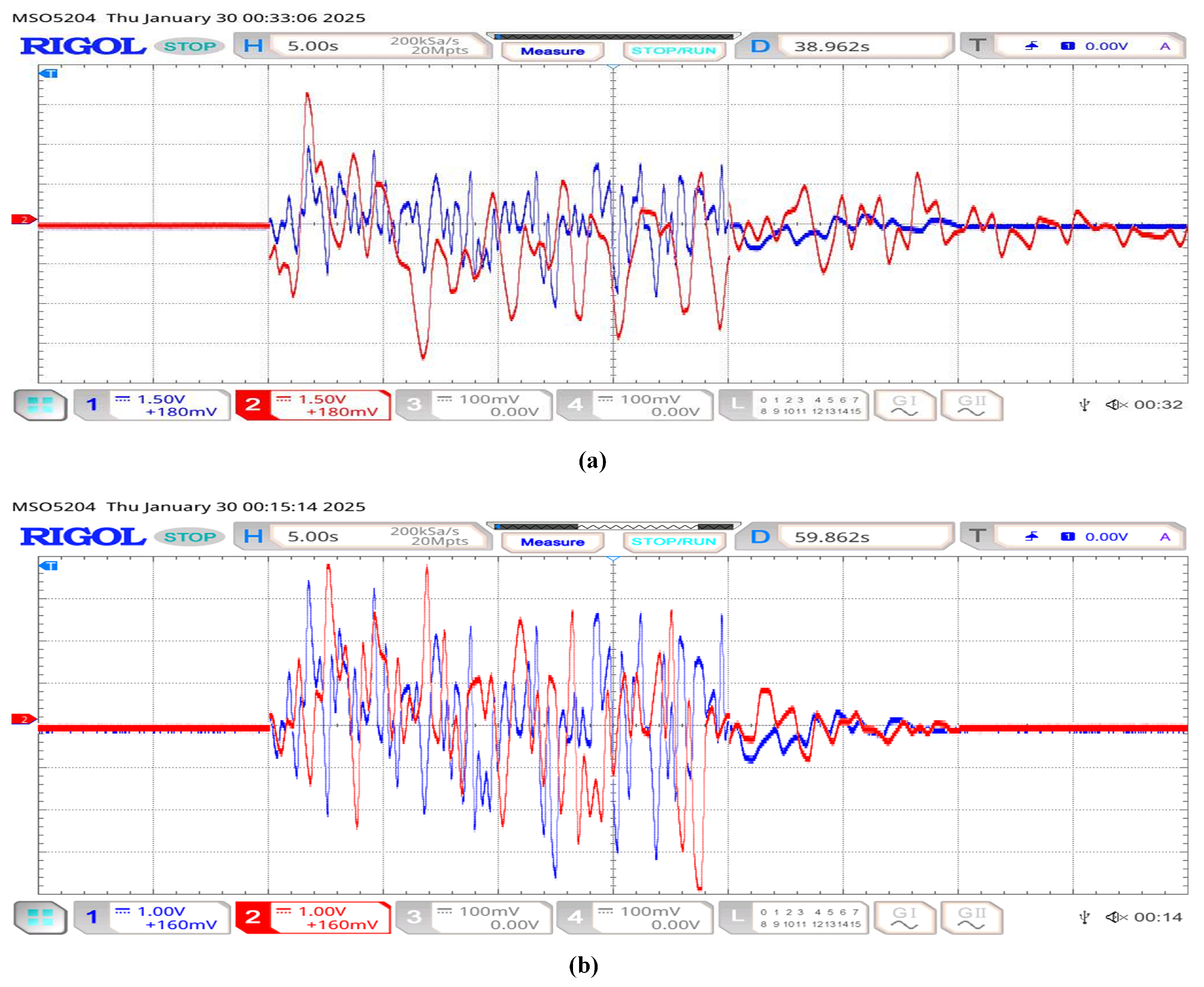
To validate the proposed LFC strategy under real-time conditions, a Hardware-in-the-Loop (HiL) experimental setup is implemented using the OPAL-RT 4512 real-time simulator and a Texas Instruments (TI) microcontroller.

The MATLAB/Simulink-based LFC model is deployed on the OPAL-RT platform via RT-LAB, and the controller is implemented on a microcontroller (Texas Instruments, Dallas, TX, USA) using Code Composer Studio. The complete hardware setup appears in Figure 12. Real-time performance is evaluated under random load disturbances that mirror the MATLAB 2023a simulations, and a digital storage oscilloscope captures the OPAL-RT frequency responses. As reported in Table 10, the HIL metrics are slightly higher than the Simulink metrics. This occurs because the Simulink signals are amplified to lie within $\pm 16$ for OPAL-RT processing and are then attenuated back to their original range before they appear on the DSO. This scaling can hide small variations in the DSO traces, while the computed statistics still register them. The experimental responses in Figure 13 closely match the Simulink responses, confirming the proposed controller’s reliability in real-time operation.

5. Conclusions

This study addressed the LFC problem in a hybrid power system by proposing a novel MWA-tuned 2DOF-FOPTID+1 controller. Integrating Aggregated Electric Vehicle (AEV) models as controllable storage units further improved the system’s resilience by actively reducing frequency and tie-line power deviations. The case study results explicitly highlight the performance improvements of this novel approach. During both step and random load variations, the proposed controller demonstrated superior damping, achieved significantly faster settling times, and minimized transient overshoots compared to conventional methods. Furthermore, sensitivity analyses and real-time OPAL-RT hardware-in-the-loop tests confirmed the controller’s robust performance under parameter variations and verified its practical feasibility. Overall, the proposed method provides a highly effective solution for improving the dynamic stability of microgrid-integrated systems.

Future work will explore secure coordination using blockchain-assisted LFC and hybrid AI techniques to improve constraint handling. Additionally, the effectiveness of AEV support during communication delays and the coordination of distributed resources across multi-area systems will be investigated.

References

1. Kechida, A.; Gozim, D.; Toual, B.; Alharthi, M.M.; Agajie, T.F.; Ghoneim, S.M.S.; Ghaly, R.N.R. Smart control and management for a renewable energy based stand-alone hybrid system. Sci. Rep. 2024, 14, 26857. [Google Scholar] [CrossRef] [PubMed]
2. Agajie, T.F.; Ali, A.; Fopah-Lele, A.; Amoussou, I.; Khan, B.; Velasco, C.L.R.; Tanyi, E. A Comprehensive Review on Techno-Economic Analysis and Optimal Sizing of Hybrid Renewable Energy Sources with Energy Storage Systems. Energies 2023, 16, 642. [Google Scholar] [CrossRef]
3. Kamarposhti, M.A.; Colak, I.; Shokouhandeh, H.; Iwendi, C.; Padmanaban, S.; Band, S.S. Optimum operation management of microgrids with cost and environment pollution reduction approach considering uncertainty using multi-objective NSGAII algorithm. IET Renew. Power Gener. 2025, 19, 274–292. [Google Scholar] [CrossRef]
4. Amoussou, I.; Tanyi, E.; Ali, A.; Agajie, T.F.; Khan, B.; Brito Ballester, J.; Nsanyuy, W.B. Optimal Modeling and Feasibility Analysis of Grid-Interfaced Solar PV/Wind/Pumped Hydro Energy Storage Based Hybrid System. Sustainability 2023, 15, 1222. [Google Scholar] [CrossRef]
5. Makahleh, F.M.; Amer, A.; Manasrah, A.A.; Attar, H.; Solyman, A.A.A.; Kamarposhti, M.A.; Thounthong, P. Optimal Management of Energy Storage Systems for Peak Shaving in a Smart Grid. Comput. Mater. Contin. 2023, 74, 3317–3334. [Google Scholar] [CrossRef]
6. Agajie, T.F.; Khan, B.; Amoussou, I.; Awoke, Y.A. Chapter 6—Impact of battery energy storage system integration on microgrid reliability improvement. In Active Electrical Distribution Network; Smart Microgrid Components; Academic Press: Cambridge, MA, USA, 2022; pp. 137–165. [Google Scholar] [CrossRef]
7. Annamraju, A.; Nandiraju, S. Coordinated control of conventional power sources and PHEVs using jaya algorithm optimized PID controller for frequency control of a renewable penetrated power system. Prot. Control Mod. Power Syst. 2019, 4, 28. [Google Scholar] [CrossRef]
8. Sondhi, S.; Hote, Y.V. Fractional order PID controller for load frequency control. Energy Convers. Manag. 2014, 85, 343–353. [Google Scholar] [CrossRef]
9. Ismayil, C.; Sreerama Kumar, R.; Sindhu, T.K. Automatic generation control of single area thermal power system with fractional order PID (PIλDμ) controllers. IFAC Proc. Vol. 2014, 47, 552–557. [Google Scholar] [CrossRef]
10. Gupta, N.K.; Kar, M.K.; Singh, A.K. Design of a 2-DOF-PID controller using an improved sine–cosine algorithm for load frequency control of a three-area system with nonlinearities. Prot. Control Mod. Power Syst. 2022, 7, 73. [Google Scholar] [CrossRef]
11. Saikia, L.C.; Sinha, N. Load frequency control of multi-area hybrid power system using symbiotic organisms search optimized two degree of freedom controller. Int. J. Renew. Energy Res. 2017, 7, 1663–1674. [Google Scholar] [CrossRef]
12. Ojha, S.K.; Maddela, C.O. Load frequency control of a two-area power system with renewable energy sources using brown bear optimization technique. Electr. Eng. 2024, 106, 3217–3231. [Google Scholar] [CrossRef]
13. Güler, Y.; Kaya, I. Load Frequency Control of Single-Area Power System with PI–PD Controller Design for Performance Improvement. J. Electr. Eng. Technol. 2023, 18, 2633–2645. [Google Scholar] [CrossRef]
14. Cui, M.; Zhao, Y.; Cao, P.; Tang, Y.; Lu, Y. Load frequency control of interconnected hydrothermal power system based on FOPI + FOPD controller. Int. J. Dyn. Control 2024, 12, 1073–1085. [Google Scholar] [CrossRef]
15. Çelik, E. Design of new fractional order PI–fractional order PD cascade controller through dragonfly search algorithm for advanced load frequency control of power systems. Soft Comput. 2021, 25, 1193–1217. [Google Scholar] [CrossRef]
16. Sahoo, S.; Jena, N.; Ray, P.; Sahu, B. Selfish Herd Optimisation tuned fractional order cascaded controllers for AGC Analysis. Soft Comput. 2022, 26, 3265–3289. [Google Scholar] [CrossRef]
17. Sekyere, Y.O.M.; Effah, F.B.; Okyere, P.Y. Optimally tuned cascaded FOPI-FOPIDN with improved PSO for load frequency control in interconnected power systems with RES. J. Electr. Syst. Inf. Technol. 2024, 11, 26. [Google Scholar] [CrossRef]
18. Murali, S.; Shankar, R. Impact of Inertia Emulation Based Modified HVDC Tie-Line for AGC Using Novel Cascaded Fractional Order Controller in Deregulated Hybrid Power System. J. Electr. Eng. Technol. 2021, 16, 1859–1875. [Google Scholar] [CrossRef]
19. Hussain, J.; Zou, R.; Pathak, P.K.; Karni, A.; Akhtar, S. Design of a novel cascade PI-(1+FOPID) controller to enhance load frequency control performance in diverse electric power systems. Electr. Power Syst. Res. 2025, 243, 111488. [Google Scholar] [CrossRef]
20. Hussain, J.; Zou, R.; Akhtar, S.; Abouda, K.A. Design of cascade P-P-FOPID controller based on marine predators algorithm for load frequency control of electric power systems. Electr. Eng. 2025, 107, 809–827. [Google Scholar] [CrossRef]
21. Shayeghi, H.; Rahnama, A.; Bizon, N. TFODn-FOPI multi-stage controller design to maintain an islanded microgrid load-frequency balance considering responsive loads support. IET Gener. Transm. Distrib. 2023, 17, 2493–2510. [Google Scholar] [CrossRef]
22. Murali, S.; Saini, P.; Abhinav, K.; Shankar, R.; Parida, S.K. Improved LSTM-Based Load Forecasting Embedded 3DOF (FOPI)-FOPD Controller for Proactive Frequency Regulation in Power System. IEEE Trans. Ind. Appl. 2024, 60, 8213–8227. [Google Scholar] [CrossRef]
23. Mohanty, P.; Sahu, R.K.; Pradhan, P.C.; Panda, S. Design and analysis of the 2DOF-PIDN-FOID controller for frequency regulation of the electric power systems. Int. J. Ambient Energy 2022, 43, 2533–2549. [Google Scholar] [CrossRef]
24. Liu, T.; Chen, A.; Gao, F.; Liu, X.; Li, X.; Hu, S. Double-Loop Control Strategy with Cascaded Model Predictive Control to Improve Frequency Regulation for Islanded Microgrids. IEEE Trans. Smart Grid 2022, 13, 3954–3967. [Google Scholar] [CrossRef]
25. Mu, C.; Tang, Y.; He, H. Improved Sliding Mode Design for Load Frequency Control of Power System Integrated an Adaptive Learning Strategy. IEEE Trans. Ind. Electron. 2017, 64, 6742–6751. [Google Scholar] [CrossRef]
26. Tummala, A.S.L.V.; Inapakurthi, R.; Ramanarao, P.V. Observer based sliding mode frequency control for multi-machine power systems with high renewable energy. J. Mod. Power Syst. Clean Energy 2018, 6, 473–481. [Google Scholar] [CrossRef]
27. Kumar, N.; Malik, H.; Singh, A.; Alotaibi, M.A.; Nassar, M.E. Novel Neural Network-Based Load Frequency Control Scheme: A Case Study of Restructured Power System. IEEE Access 2021, 9, 164917–164932. [Google Scholar] [CrossRef]
28. Bevrani, H.; Daneshmand, P.R. Fuzzy Logic-Based Load-Frequency Control Concerning High Penetration of Wind Turbines. IEEE Syst. J. 2012, 6, 173–180. [Google Scholar] [CrossRef]
29. Yousef, H.A.; Al-Kharusi, K.; Albadi, M.H.; Hosseinzadeh, N. Load Frequency Control of a Multi-Area Power System: An Adaptive Fuzzy Logic Approach. IEEE Trans. Power Syst. 2014, 29, 1822–1830. [Google Scholar] [CrossRef]
30. Su, J.; Zhang, H.; Liu, H.; Liu, D. Lyapunov-based distributed secondary frequency and voltage control for distributed energy resources in islanded microgrids with expected dynamic performance improvement. Appl. Energy 2025, 377, 124539. [Google Scholar] [CrossRef]
31. García-Pereira, H.; Blanco, M.; Martínez-Lucas, G.; Pérez-Díaz, J.I.; Sarasúa, J.I. Comparison and Influence of Flywheels Energy Storage System Control Schemes in the Frequency Regulation of Isolated Power Systems. IEEE Access 2022, 10, 36077–36087. [Google Scholar] [CrossRef]
32. Kumar, D.; Bhushan, R. Improving the dynamic response of frequency and power in a wind integrated power system by optimal design of compensated superconducting magnetic energy storage. Int. J. Green Energy 2018, 15, 223–234. [Google Scholar] [CrossRef]
33. Cui, S.; Yan, X. Inertia and primary frequency modulation strategy for a doubly fed induction generator based on supercapacitor energy storage control. Int. J. Green Energy 2022, 19, 1549–1562. [Google Scholar] [CrossRef]
34. Elkasem, A.H.A.; Kamel, S.; Khamies, M.; Nasrat, L. Frequency regulation in a hybrid renewable power grid: An effective strategy utilizing load frequency control and redox flow batteries. Sci. Rep. 2024, 14, 9576. [Google Scholar] [CrossRef] [PubMed]
35. Xiang, B.; Mao, X.; Liu, Z.; Wang, H. Stabilization of isolated hybrid microgrids with electric vehicle-based energy storage systems using a fractional order proportional-integral-derivative control. Int. J. Green Energy 2024, 21, 1364–1379. [Google Scholar] [CrossRef]
36. Thorat, R.; Bhatt, P. Electric vehicle participation for optimized load frequency control in a multi-area restructured power system. Int. J. Model. Simul. 2026, 46, 182–195. [Google Scholar] [CrossRef]
37. Knez, K.; Herman, L.; Blažič, B. Dynamic Management of Flexibility in Distribution Networks through Sensitivity Coefficients. Energies 2024, 17, 1783. [Google Scholar] [CrossRef]
38. Yang, H.; Tang, K.; Ma, J.; Zhang, D.; Qi, X. Energy and flexibility markets clearing mechanism for electrical distribution system through a flexibility imbalance modification strategy. Int. J. Electr. Power Energy Syst. 2026, 177, 111862. [Google Scholar] [CrossRef]
39. Villar, J.; Bessa, R.; Matos, M. Flexibility products and markets: Literature review. Electr. Power Syst. Res. 2018, 154, 329–340. [Google Scholar] [CrossRef]
40. Bhagat, S.K.; Saikia, L.C. Application of inertia emulation control strategy with energy storage system in multi-area hydro-thermal system using a novel metaheuristic optimized tilt controller. Electr. Power Syst. Res. 2023, 222, 109522. [Google Scholar] [CrossRef]
41. Sariki, M.; Shankar, R. Optimal CC-2DOF(PI)-PDF controller for LFC of restructured multi-area power system with IES-based modified HVDC tie-line and electric vehicles. Eng. Sci. Technol. Int. J. 2022, 35, 101099. [Google Scholar] [CrossRef]
42. Choudhary, R.; Rai, J.N.; Arya, Y. FOPTID+1 controller with capacitive energy storage for AGC performance enrichment of multi-source electric power systems. Electr. Power Syst. Res. 2023, 221, 109450. [Google Scholar] [CrossRef]
43. Mohanty, B.; Panda, S.; Hota, P.K. Controller parameters tuning of differential evolution algorithm and its application to load frequency control of multi-source power system. Int. J. Electr. Power Energy Syst. 2014, 54, 77–85. [Google Scholar] [CrossRef]
44. Khokhar, B.; Dahiya, S.; Parmar, K.P.S. A Robust Cascade Controller for Load Frequency Control of a Standalone Microgrid Incorporating Electric Vehicles. Electr. Power Compon. Syst. 2020, 48, 435–448. [Google Scholar] [CrossRef]
45. Crowe, J.; Tan, K.K.; Lee, T.H.; Ferdous, R.; Katebi, M.R.; Huang, H.-P.; Jeng, J.-C.; Tang, K.S.; Chen, G.R.; Man, K.F.; et al. PID Control: New Identification and Design Methods; Johnson, M.A., Moradi, M.H., Eds.; Springer: Berlin/Heidelberg, Germany, 2005. [Google Scholar]
46. Oustaloup, A.; Levron, F.; Mathieu, B.; Nanot, F.M. Frequency Band Complex Noninteger Differentiator: Characterization and Synthesis. IEEE Trans. Circuits Syst. I Fundam. Theory Appl. 2000, 47, 25–39. [Google Scholar] [CrossRef]
47. Agajie, T.F.; Ibrahim, F.S.; Amoussou, I.; Agajie, E.F.; Paddy, E.Y.; Awoke, Y.A.; Nsanyuy, W.B.; Bajaj, M. Comparative techno-economic analysis of grid-connected solar PV-battery and PV-fuel cell systems for educational institutions sustainable academic laboratories. Discov. Sustain. 2025, 6, 14. [Google Scholar] [CrossRef]
48. Agajie, T.F.; Fopah-Lele, A.; Ali, A.; Amoussou, I.; Khan, B.; Elsisi, M.; Nsanyuy, W.B.; Mahela, O.P.; Álvarez, R.M.; Tanyi, E. Integration of Superconducting Magnetic Energy Storage for Fast-Response Storage in a Hybrid Solar PV-Biogas with Pumped-Hydro Energy Storage Power Plant. Sustainability 2023, 15, 10736. [Google Scholar] [CrossRef]
49. Agajie, T.F.; Fopah-Lele, A.; Amoussou, I.; Ali, A.; Khan, B.; Tanyi, E. Optimal Design and Mathematical Modeling of Hybrid Solar PV–Biogas Generator with Energy Storage Power Generation System in Multi-Objective Function Cases. Sustainability 2023, 15, 8264. [Google Scholar] [CrossRef]
50. Mojtahedzadeh Larijani, M.; Ahmadi Kamarposhti, M.; Nouri, T. Stochastic Unit Commitment Study in a Power System with Flexible Load in Presence of High Penetration Renewable Farms. Int. J. Energy Res. 2023, 2023, 9979610. [Google Scholar] [CrossRef]
51. Trojovský, P.; Dehghani, M. A new bio-inspired metaheuristic algorithm for solving optimization problems based on walruses behavior. Sci. Rep. 2023, 13, 8775. [Google Scholar] [CrossRef] [PubMed]
52. Mahdavi, S.; Rahnamayan, S.; Deb, K. Opposition based learning: A literature review. Swarm Evol. Comput. 2018, 39, 1–23. [Google Scholar] [CrossRef]
53. Zhao, S.; Zhang, T.; Ma, S.; Wang, M. Sea-horse optimizer: A novel nature-inspired meta-heuristic for global optimization problems. Appl. Intell. 2023, 53, 11833–11860. [Google Scholar] [CrossRef]
54. Abdollahzadeh, B.; Gharehchopogh, F.S.; Khodadadi, N.; Mirjalili, S. Mountain Gazelle Optimizer: A new Nature-inspired Metaheuristic Algorithm for Global Optimization Problems. Adv. Eng. Softw. 2022, 174, 103282. [Google Scholar] [CrossRef]
55. Ahmadi Kamarposhti, M.; Shokouhandeh, H.; Gholami Omali, Y.; Colak, I.; Thounthong, P.; Holderbaum, W. Optimal Coordination of TCSC and PSS2B Controllers in Electric Power Systems Using MOPSO Multiobjective Algorithm. Int. Trans. Electr. Energy Syst. 2022, 2022, 5233620. [Google Scholar] [CrossRef]
56. Izadkhast, S.; Garcia-Gonzalez, P.; Frías, P. An Aggregate Model of Plug-In Electric Vehicles for Primary Frequency Control. IEEE Trans. Power Syst. 2015, 30, 1475–1483. [Google Scholar] [CrossRef]
57. Wang, B.; Zhao, D.; Dehghanian, P.; Tian, Y.; Hong, T. Aggregated Electric Vehicle Load Modeling in Large-Scale Electric Power Systems. IEEE Trans. Ind. Appl. 2020, 56, 5796–5810. [Google Scholar] [CrossRef]
Figure 1. Hybrid two-area power system.
Energies 19 03401 g001
Figure 2. Block diagram of proposed controller.
Energies 19 03401 g002
Figure 3. Convergence curves with various optimization techniques.
Energies 19 03401 g003
Figure 4. Eigen values on s-plane.
Energies 19 03401 g004
Figure 5. Comparison of system frequency responses using the proposed controller and existing state-of-the-art techniques. (a) Area 1 frequency deviations (b) Area 2 frequency deviations.
Energies 19 03401 g005
Figure 6. Linearized Model of Aggregated Electric Vehicle.
Energies 19 03401 g006
Figure 7. Comparison of frequency deviations after AEV integration with proposed controller. (a) Area 1 frequency deviations (b) Area 2 frequency deviations.
Energies 19 03401 g007
Figure 8. Sensitivity analysis: system responses under parameter variations using proposed controller. (a) Area 1 frequency deviations (b) Area 2 frequency deviations.
Energies 19 03401 g008
Figure 9. Sensitivity analysis: system responses under multi parameter variations with proposed controller. (a) Area 1 frequency deviations with two parameter variation (b) Area 2 frequency deviations with two parameter variation (c) Area 1 frequency deviations with three parameter variation (d) Area 2 frequency deviations with three parameter variation.
Energies 19 03401 g009
Figure 10. Frequency deviations using the proposed controller for random solar input (a) Random solar irradiation (b) Area 1 frequency deviations (c) Area 2 frequency deviations.
Energies 19 03401 g010
Figure 11. Responses with random load deviations using the proposed controller (a) Area 1 frequency deviations (b) Area 2 frequency deviations.
Energies 19 03401 g011
Figure 12. Hardware setup for real-time analysis.
Energies 19 03401 g012
Figure 13. Real-time responses obtained using OPAL-RT (where blue represents with AEV and red represents without AEV): (a) Area 1 frequency deviations, (b) Area 2 frequency deviations.
Energies 19 03401 g013