A Novel Fault Location Method for MMC-HVDC Grid Based on Gram Angle Difference Field

Abstract

When a short-circuit fault occurs along the transmission line of a modular multilevel converter high-voltage direct-current (MMC-HVDC) grid, the sub-module capacitors discharge, causing the fault current to rapidly rise, posing a threat to the safe operation of the system. Therefore, this paper proposes a novel fault location method based on the Gram Angle Difference Field (GADF). The column corresponding to the maximum differential value in a sliding window is used to identify the fault moment and locate faults in MMC-HVDC transmission lines. In order to effectively distinguish normal fluctuations from fault mutations and avoid false alarms, a dynamic threshold is set based on the statistical characteristics of normal data. This method utilizes the unique feature extraction capability of the GADF matrix, the adaptive mechanism of the dynamic threshold, and the stability of line-mode voltage to achieve fast and accurate fault location. Finally, this method is validated using a simulation model. The results show that the proposed method can accurately locate faults in different conditions.

1. Introduction

The MMC-HVDC system has the advantages of flexible operation, fast response, strong controllability, low harmonic levels, and no commutation failure [1,2,3,4,5]. As a result, it has attracted extensive attention and research. When a fault occurs on the DC side of the MMC-HVDC, the discharge of sub-module (SM) capacitors generates a large fault current [6,7,8,9]. Therefore, when a fault occurs, rapid and accurate fault location is very important.

Researchers have proposed various methods, including the traveling wave (TW) method, fault analysis method, and intelligent algorithms [10,11,12]. The TW method is widely used because of its fast response speed and independence from system parameters. However, the accuracy is influenced by the sampling frequency and the accuracy of the TW velocity estimation. To overcome the influence of sampling frequency, reference [13] uses a frequency correction algorithm to correct the frequency distortion of the TW. Reference [14] optimizes the fault location formula by introducing a probability search field component. To improve the accuracy of the TW velocity estimation, reference [15] analyzes the TW to obtain the frequency correlation characteristics of the wave velocity. However, these improvements introduce additional computational complexity. In addition, optimizing the TW method using experimental equipment will increase hardware costs and field deployment difficulty [16,17]. Despite these efforts, some key challenges remain, and the location accuracy is still affected by high-impedance faults and strong noise environments. Fault analysis-based methods locate faults by analyzing the fault characteristics of voltage or current [18,19,20,21]. These methods require accurate extraction of the characteristics of specific frequency components of the fault signal and then analysis of the fault data. Their accuracy is highly dependent on the quality and completeness of the data, and is usually sensitive to transition resistance and noise. Methods based on intelligent algorithms have also been extensively studied. Data fitting, least squares, and other algorithms have been used to improve the estimation accuracy of wave velocity [22,23]. Hilbert–Huang transform (HHT), variational mode decomposition (VMD), signal segmentation, and other algorithms have been used to improve wavefront identification [24,25,26]. However, these methods have obvious limitations. Wavelet transform, through multi-scale decomposition, achieves high-frequency feature extraction of faults and has been widely used in early HVDC fault detection and location research. However, its analytical performance depends on the selection of the mother wavelet function, and it is difficult to guarantee optimal results under different operating conditions. To improve time-frequency resolution, S-transform achieves joint time–frequency analysis while preserving phase information, which can more accurately describe the transient process of faults, but its computational complexity is high. Subsequently, HHT uses empirical mode decomposition to achieve adaptive signal analysis, overcoming the limitation of fixed basis functions, but it suffers from mode aliasing and endpoint effects. To address this deficiency, VMD improves mode separation capability through a variational optimization framework, but its performance depends on parameter settings. Therefore, while existing time–frequency analysis methods have improved fault feature extraction capabilities, they still have limitations in terms of parameter sensitivity, noise resistance, and feature stability. Unlike traditional signal processing methods, GADF, as a data-driven transform, does not require predefined basis functions, thus avoiding the basis function dependency problem of wavelet transforms. Furthermore, the proposed method does not perform mode decomposition of the signal, fundamentally eliminating the inherent mode aliasing defects of methods such as HHT and VMD. This method requires only simple polar coordinate transformation and angle difference matrix calculation, without complex parameter tuning. By combining a dynamic threshold based on the 3σ principle and first-order differential detection, this method can accurately capture fault abrupt changes even under extreme conditions of a 20 dB signal-to-noise ratio (SNR) and a 500 Ω fault resistance. The entire location process is based on matrix operations, requiring no iteration, resulting in high computational efficiency and meeting the real-time requirements of practical engineering.

The remainder is organized as follows. Section 2 presents the principle of TW fault location; Section 3 proposes a novel method based on GADF and differential features; Section 4 validates this method through simulation models; and Section 5 provides a conclusion for the proposed method.

2. TW Fault Location Principle

2.1. Decoupling and Line-Mode Selection of MMC-HVDC Grid

For bipolar MMC-HVDC grids, considering the coupling problem, decoupling is required. The transient voltage TW is decomposed into the line mode and zero mode [27],

$$\left[\begin{array}{c}{u}_0\\ u_1\end{array}\right]={\displaystyle \frac{1}{\sqrt{2}}}\left[\begin{array}{cc}1& 1\\ 1& -1\end{array}\right]\cdot \left[\begin{array}{c}{u}_p\\ u_n\end{array}\right]$$

(1)

where $u_0$ is the zero mode, $u_1$ is the line mode, $u_p$ is positive, and $u_n$ is negative.

The line parameters of grids with different modes are different, reflecting the differences in the physical characteristics of the grid modes. The zero mode has serious attenuation and significant frequency variation, which leads to large TW loss and unstable wave velocity [28]. In contrast, the line-mode wave velocity varies very little with frequency, and is close to the speed of light in both low-frequency and high-frequency bands. In addition, the line mode has other advantages. On the one hand, the line mode can effectively suppress zero-mode interference and is not affected by the grounding method, and has stronger adaptability and robustness. Moreover, in the case of positive-to-negative pole (P-N) short-circuit faults, the zero mode is approximately zero, while the line mode shows significant mutation features. Therefore, the selection of the line mode for research can not only ensure applicability under different fault types, but also improve the accuracy and reliability.

2.2. Two-Terminal TW Method

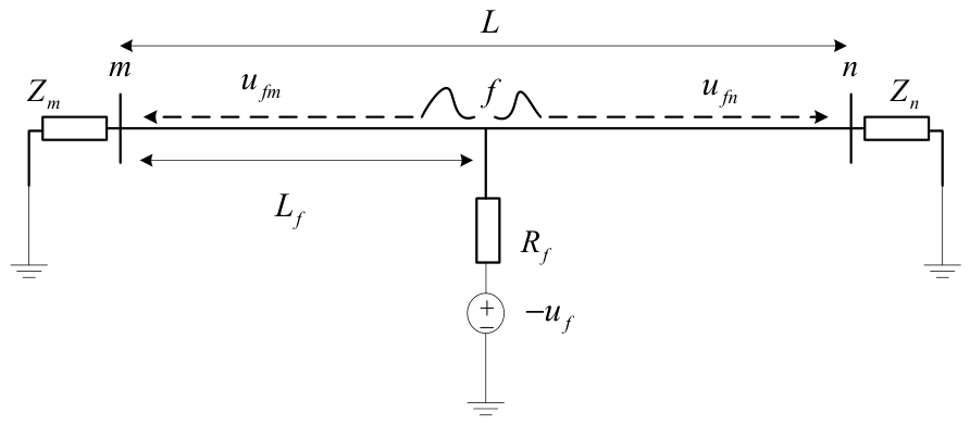
Figure 1 shows the equivalent circuit for a positive-to-ground model (P-G); this model is used to analyze the fault location principle of two-terminal TWs. The initial fault TW propagates from the fault point to both terminals.

Figure 1. MMC-HVDC transmission line.

Figure 1. MMC-HVDC transmission line.

where f is the fault location, Z_m and Z_n are the system impedances, R_f is the fault resistance, $u_f$ is the normal voltage, $u_{fm}$ and $u_{fn}$ are the initial fault TWs.

The proposed method is based on the two-terminal TW method for fault location, which only requires accurate identification of the initial wavefront of the fault TW. The fault location can be more accurately calculated based on the arrival time of the initial wavefronts at both terminals.

$$L_f=v\cdot (t_m-t_0)$$

(2)

$$L_f=v\cdot (t_m-t_0)$$

(3)

$$L_f={\displaystyle \frac{L+v\cdot (t_m-t_n)}{2}}$$

(4)

where L_f is the fault distance, $t_m$ and $t_n$ are the times when the initial fault TW arrives at both ends, and $v$ is the wave velocity. The $v$ of the linear mode varies minimally with frequency and remains essentially constant in the high-frequency range. Therefore, this paper selects a fixed wave velocity of 2.97 × 10⁸ m/s.

Time synchronization is crucial for achieving high accuracy [29]. GPS provides nanosecond-level timing accuracy that meets these requirements, thereby effectively improving precision.

3. Fault Location Method Based on GADF and Differential Features

Short-circuit faults in MMC-HVDC systems can cause sudden changes in voltage and current, which are typical time series data. The GADF converts time series into images, preserving their temporal information and dynamic features, making it suitable for capturing sudden changes at the moment of a fault. GADF can capture sudden changes in time series by observing changes in angle differences, thereby identifying the moment of fault occurrence.

3.1. Gram Angle Difference Field

GADF implementation steps:

(1)

Assume that the input one-dimensional time series signal is X. First, normalize it:

$$\widehat{x}={\displaystyle \frac{\left(x_i-\max \left(X\right)\right)+\left(x_i-\min \left(X\right)\right)}{\max \left(X\right)-\min \left(X\right)}}$$

(5)

(2)

Convert the scaled data into polar coordinates, using the data values as the angular component, and encode the corresponding timestamp as the radius.

$$\left\{\begin{array}{l}{\theta }_i=\arccos \left({\widehat{x}}_i\right)-1\le {\widehat{x}}_i\le 1,{\widehat{x}}_i\in \widehat{X}\\ r_i={\displaystyle \frac{t_i}{M}}{t}_i\in M\end{array}\right.$$

(6)

where t_i is the timestamp, and M is the constant factor of the span of the regularized polar coordinate system.

(3)

The normalized data has been transformed into polar coordinates and encapsulates temporal information, so it can be reconstructed using GADF.

$$\begin{array}{cc}\hfill GADF=& [\sin ({\theta }_i-{\theta }_j)]\hfill \\ \hfill =& \sqrt{1-{\widehat{X}}^2}\cdot {(\widehat{X})}^{\mathrm{T}}-\widehat{X}\cdot {(\sqrt{1-{\widehat{X}}^2})}^{\mathrm{T}}\hfill \end{array}$$

(7)

where X is the time series signal and T is the transposition calculation.

3.2. Fault Location Method

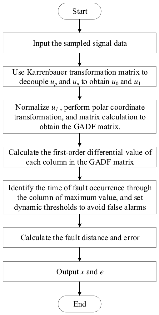
When a fault occurs in the DC side, the transient voltage contains a significant amount of high-frequency fault signals. This paper focuses on accurately extracting useful information from these signals and using this information for fault location. A method employing the GADF is proposed to decompose the fault signal and identify the fault occurrence moment using the first-order difference of the GADF matrix for fault location. The proposed method uses the advantages of the GADF in achieving high-precision fault location. Figure 2 illustrates the flowchart of this method.

The operation steps are:

Step 1: Establish a simulation model and set short-circuit faults on transmission lines. Real-time sampling of fault voltage.

Step 2: Decompose the transient voltages using the Karrenbauer transformation. Select the line-mode component that is relatively stable with frequency for subsequent analysis.

Step 3: Calculate the GADF matrix. First, normalize the line-mode voltage, then convert the scaled data to polar coordinates. Using a sliding window approach with 10 data points per time window, perform matrix calculations on the fault data within the window to generate a local GADF matrix.

Step 4: Calculate the first-order difference of the GADF matrix along the column directions, and find the column with the largest absolute difference value. In order to effectively distinguish normal fluctuations from fault mutations and avoid false alarms, a dynamic threshold is set based on the statistical characteristics of normal data. The threshold adopts the 3σ principle. Under normal operation, the differential signal approximately obeys the Gaussian distribution. Therefore, if the differential value exceeds this range, it can be determined as a mutation point. The dynamic threshold set in this way can adapt to different noise levels and signal strengths. When the noise is large, the threshold increases as σ increases to avoid misjudgment. When the signal quality is good, the threshold becomes more sensitive as σ decreases. This ensures that faults can still be accurately detected under low SNR, while avoiding false alarms caused by noise or normal fluctuations under high SNR. If the differential value exceeds the dynamic threshold and is the maximum value of the window, it is considered that a fault has occurred and the calculation process of the sliding window is stopped. Otherwise, the time window is moved and the above steps are repeated until the fault is detected. By combining this sliding window with a dynamic threshold, the fault signal mutation characteristics can be efficiently captured while improving real-time performance and robustness.

The dynamic threshold is

$$T=\mu +3\sigma$$

(8)

$$\mu ={\displaystyle \frac{1}{N}}{\displaystyle \sum _{i=1}^N{x}_i}$$

(9)

$$\sigma =\sqrt{{\displaystyle \frac{1}{N}}{\displaystyle \sum _{i=1}^N{(x_i-\mu )}^2}}$$

(10)

where μ is the mean and σ is the standard deviation.

For a set of discrete sequences {x₁, x₂ … x_n}, its first-order difference sequence is

$$\Delta x_i=x_i-x_{i-1} (i=2,3,\dots ,n)$$

(11)

The calculation process is to use each element to subtract the value of the previous element, and the length of the generated new sequence is n − 1.

Step 5: Calculate the fault distance and error:

$$e={\displaystyle \frac{\left|L_{cal}-L_{act}\right|}{L}}\cdot 100\%$$

(12)

where e is the error, L_act is the actual value, and L_cal is the calculated value.

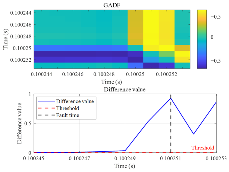
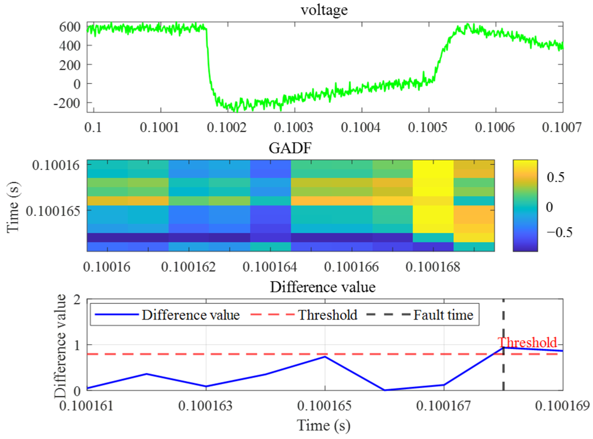
Figure 3 shows the line-mode voltage, the GADF matrix at the time of fault detection, and the difference calculated from this matrix. The horizontal and vertical axes of the GADF matrix represent actual time coordinates, and the colors represent the sine values of the angle differences. By calculating the first-order difference of the GADF matrix, the moment of fault occurrence can be identified and the fault can be located.

4. Simulation Analysis

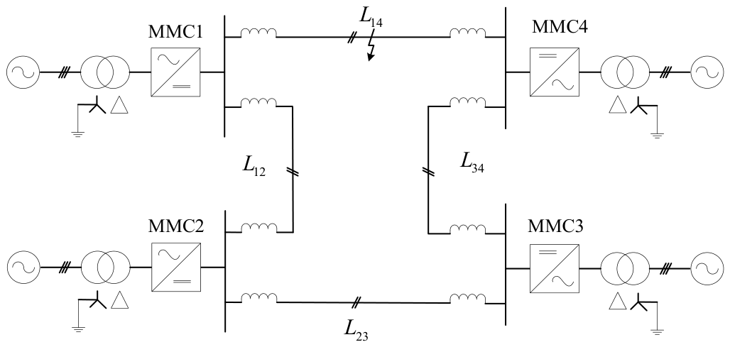
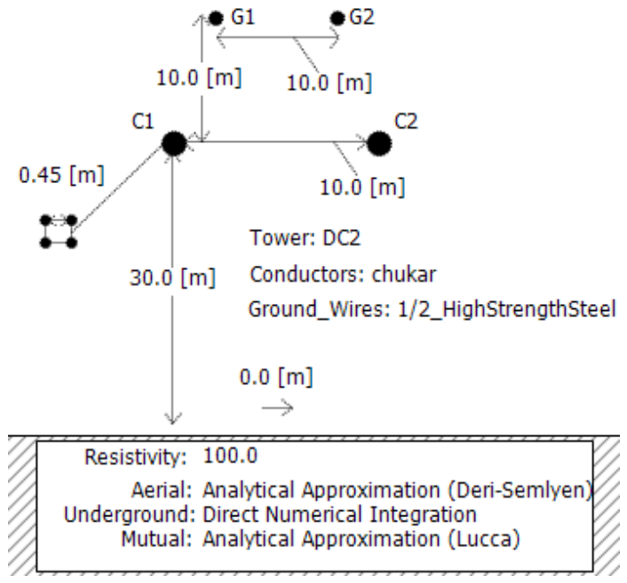
To verify the proposed method, a ±400 kV MMC-HVDC model was built in PSCAD/EMTDC, as shown in Figure 4.

Table 1. Grid parameters.

Parameters	MMC1	MMC2	MMC3	MMC4
DC voltage (kV)	±400	±400	±400	±400
Rated power (MW)	750	750	1000	1500
Control mode	P-Q	P-Q	V-Q	P-Q
Bridge arm reactor (mH)	50	50	50	50
SM capacitor (mF)	3	3	3	3
SM number	200	200	200	200

lists the key parameters. The transmission line is an overhead line based on frequency-dependent characteristics. The line structure is shown in Figure 5. The converter uses a half-bridge sub-module with voltage and current protection, which will be locked if the voltage violates the standard or the overcurrent exceeds 100 μs. Based on this model, analyze the fault location performance of the proposed method.

4.1. Impact of Fault Distance

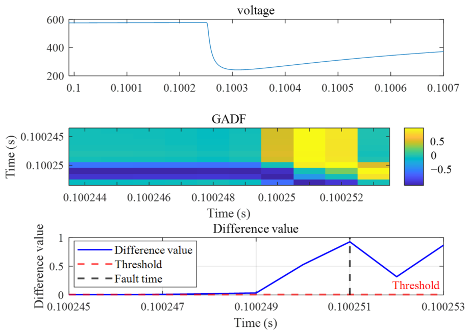
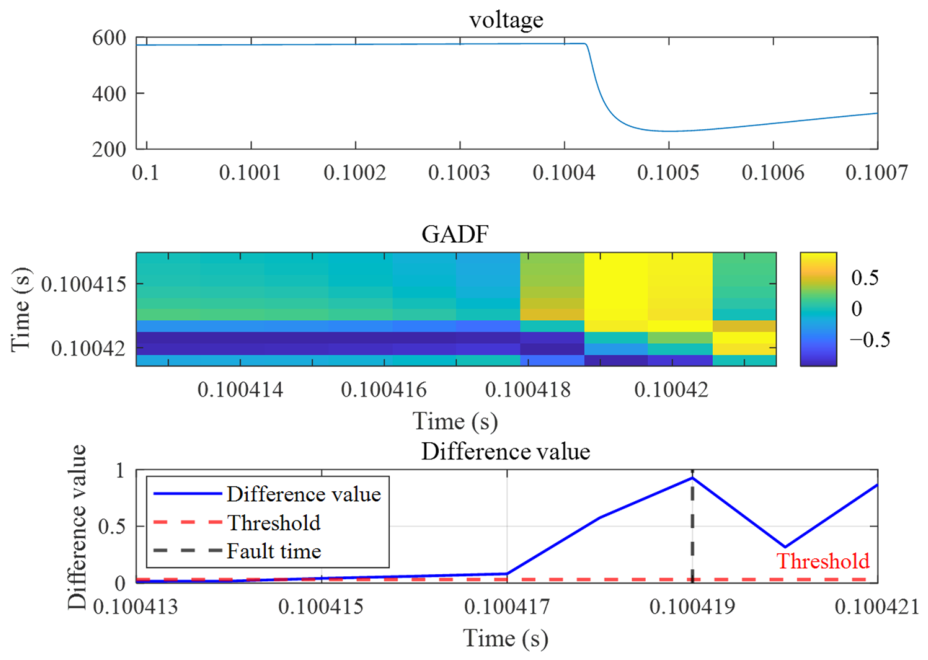
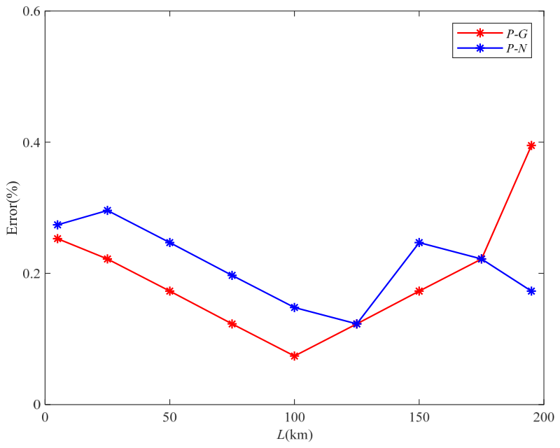
As the fault distance increases, the signal will attenuate, which will affect the fault location. To validate its impact on the proposed method, line L₁₄ with a total length of 200 km is selected for analysis. Faults are set along the transmission line. This study analyzes P-G faults and P-N faults with a fault resistance of 100 Ω, with a sampling frequency of 1 MHz. The 1 MHz is used primarily to fully capture the high-frequency transient characteristics of the initial TW of the fault and to improve the detection accuracy at the fault arrival time. Figure 6 and Figure 7 show the line-mode voltage, GADF matrix and differential value at both ends of the transmission line at a fault distance of 75 km. Figure 8 shows the fault location errors under different conditions. The results show that this method performs excellently, with a maximum error of 0.397% occurring near MMC4. At measurement points near the fault, initial wavefront identification is prone to interference from reflected waves. At the far end, the signal attenuation is significant, resulting in a weakened TW signal feature and increasing the difficulty of fault location. These factors all have a certain impact on wavefront identification. However, this method uses the global features of the angle difference matrix and a dynamic threshold to accurately identify the initial and reflected wavefronts. When the signal attenuates, the normalized angle difference still maintains similarity, reducing the influence of amplitude. By focusing on the time series mutation, the arrival time of the TW is captured.

4.2. Impact of Fault Resistance

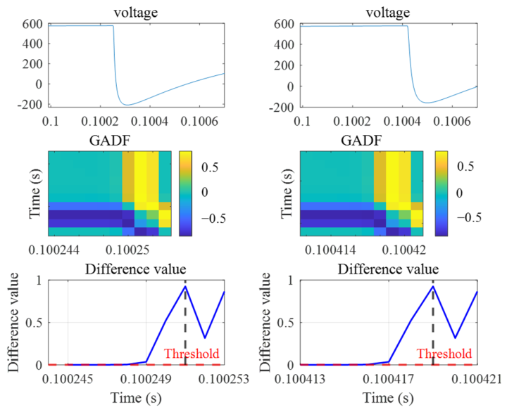
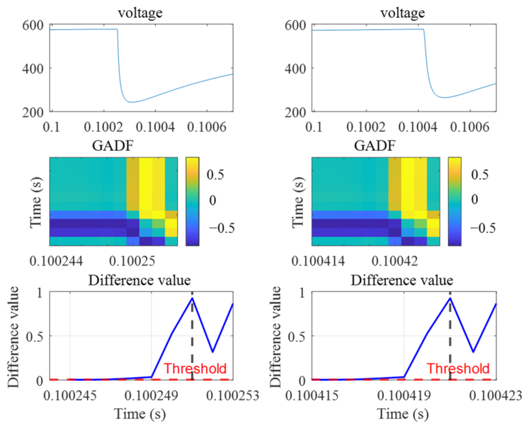
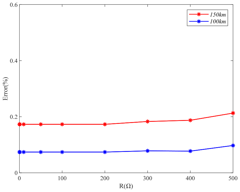
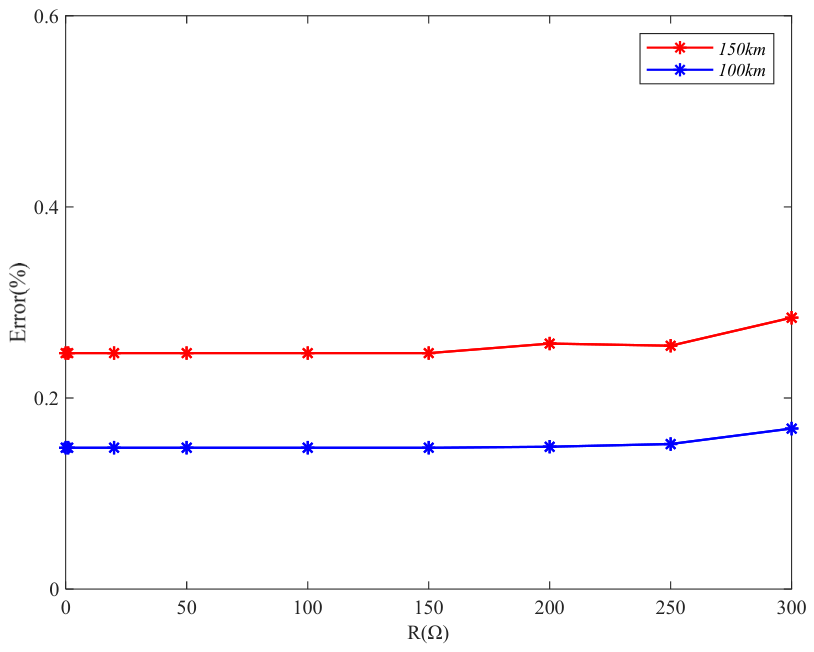
To analyze the impact of R_f, P-G and P-N are set at L₁₄ for analysis. Figure 9 shows the GADF matrix and its differential value at both ends for a P-N at 75 km. Figure 10 shows the GADF matrix and its differential value at both ends of the line for a P-G. This demonstrates the applicability of this method to different fault types. Figure 11 shows the error for different fault resistances under P-G faults. Figure 12 shows the error for different fault resistances under P-N faults. It can be seen that the proposed method demonstrates excellent fault location results for various fault resistances. This method is tolerant to high transient resistances and achieves high accuracy even at 500 Ω. This broadens the scope of its application. However, an increase in R_f leads to greater attenuation of the TW, making it particularly difficult to detect the wavefront at remote measurement points. However, this method can still identify the fault instant by focusing on the sudden change in the time series, thus maintaining high fault location accuracy.

4.3. Impact of Noise Interference

Switching noise and white noise are present in the MMC-HVDC grid. The switching noise is caused by the high-frequency switching operation of power electronic devices. It can be effectively suppressed by devices such as filters and system-level control strategies. The influence of white noise caused by random factors such as sensors and environmental noise requires further analysis. In order to verify the anti-noise ability, a Gaussian white noise signal is applied to the collected fault signal for analysis. The SNR is an indicator used to measure signal quality:

$$SNR=20\lg \left({\displaystyle \frac{Vs}{Vn}}\right)$$

(13)

where Vs is the signal and Vn is the noise.

As noise signals increase, fault time identification becomes challenging. In the MMC-HVDC system, the noise is controlled to be around 1–2% of the system’s rated voltage. Based on this standard, the analysis in this paper incorporates additive white Gaussian noise with SNRs of 50 dB, 30 dB, and 20 dB. Figure 13 shows the GADF matrix and its differential values when the SNR is 20 dB. The error shown in

Table 2. Fault location results.

Fault Type	Error (%)
	Normal	50 dB	30 dB	20 dB
50 kmP-N	0.087	0.148	0.198	0.247
50 kmP-G	0.085	0.099	0.173	0.198
100 kmP-N	0.139	0.148	0.247	0.247
100 kmP-G	0.067	0.047	0.247	0.297

indicates that this method remains effective at an SNR of 20 dB. This is because the proposed method has good noise robustness. The amplitude fluctuations caused by noise are compressed after being normalized by GADF, and fault mutations are retained through angle differences without affecting the identification of the fault time. The dynamic threshold set by the proposed method can also automatically adapt to different noise interferences. In summary, the proposed method integrates time domain, angle domain, and physical constraints to improve the anti-noise ability and meet the requirements of practical engineering applications.

4.4. Comparative Analysis

To evaluate the performance of the proposed method, this paper conducts an analysis based on two aspects: comparisons with existing literature and comparisons under standardized testing conditions. First, representative fault location methods from existing research including wavelet transform, Support Vector Regression (SVR), S-Transform, EMD, HHT, and VMD are selected for a comparative study focusing on fault location accuracy, anti-noise ability, and tolerance to fault resistance. As shown in

Table 3. Comparison results of different methods.

Method	Error (%)	SNR (dB)	Rf (Ω)
Proposed	0.176	20	500
SVR [1]	0.57	55	150
Wavelet [10]	0.46	30	300
S-Transform [15]	0.67	/	300
EMD [24]	0.50	/	100
HHT [29]	0.52	/	300
VMD [30]	0.19	/	200

, the proposed method achieves an average location error of 0.176%, demonstrating high accuracy. Furthermore, the method enables accurate fault location at an SNR of 20 dB and a fault resistance of 500 Ω, exhibiting strong anti-noise ability and tolerance to high-resistance faults. Existing studies indicate that the EMD decomposition relied upon by HHT can suffer from mode mixing in complex noise environments, thereby compromising the accuracy of fault feature extraction. While VMD mitigates mode mixing to some extent, its decomposition performance is sensitive to parameters such as the number of modes and the penalty factor [30]. Consequently, the performance of traditional signal processing methods may be constrained under complex operating conditions.

To compare performance under standardized testing conditions, this paper evaluates the proposed method against the wavelet transform and HHT methods. A P-G fault with a fault resistance of 300 Ω is set at L₁₄. Additionally, Gaussian white noise with SNRs of 50 dB and 20 dB is superimposed to evaluate the anti-noise ability of the different methods. The experimental results are presented in

Table 4. Results of different methods under the same simulation conditions.

Method	Error (%)
	Normal	50 dB	20 dB
Proposed	0.074	0.099	0.198
Wavelet	1.36	1.40	/
HHT	0.086	1.12	/

.

As shown in Table 4, under the same test conditions, the proposed method achieved the lowest fault location error. Under normal conditions and with an SNR of 50 dB, its location accuracy is superior to the wavelet transform and HHT methods. Even at an SNR of 20 dB, the proposed method successfully extracted fault features and achieved effective localization. In contrast, the wavelet transforms and HHT methods failed to yield reliable results because strong noise interference prevented the accurate determination of wavefront arrival times. This demonstrates that the proposed method has excellent potential for engineering applications.

5. Conclusions

This paper analyzes the TW characteristics of fault voltages in MMC-HVDC grids and proposes a novel fault location method based on GADF. This method demonstrates excellent performance. The conclusions are as follows:

Utilizing the GADF matrix and angle differences to mitigate the effects of noise. It utilizes first-order differences to accurately capture small mutations, making it suitable for high-noise conditions. A dynamic threshold is set based on the statistical characteristics of normal data to avoid false alarms and adapt to reflection interference and attenuation of fault signals.

To avoid coupling issues, the sampled voltages undergo Karrenbauer transformation. Line-mode voltages with stable performance are selected for analysis.

By utilizing matrix operations and first-order differences, eliminating the need for complex iterative calculations and meeting the requirements for MMC-HVDC fault location. It also exhibits strong anti-noise ability, resisting interference with an SNR of 20 dB. The proposed method uses sampled voltage signals without the need for additional equipment. It can tolerate 500 Ω fault resistance, demonstrating high engineering application value.

References

1. Farshad, M. Fault Location in Hvdc Grids Equipped with Quick-Action Protections and Circuit Breakers Based on Voltage Transient Response. IEEE Trans. Ind. Electron. 2021, 68, 12881–12889. [Google Scholar] [CrossRef]
2. Wang, B.L.; Liu, Y.; Lu, D.Y.; Yue, K.; Fan, R. Transmission Line Fault Location in Mmc-Hvdc Grids Based on Dynamic State Estimation and Gradient Descent. IEEE Trans. Power Deliv. 2021, 36, 1714–1725. [Google Scholar] [CrossRef]
3. Gao, S.P.; Song, X.C.; Ye, H.F.; Jiang, L.; Song, G.B. Transient Energy Protection Based on Wavelet Packet Transform for Hybrid Bipolar Hvdc Transmission System. IET Gener. Transm. Distrib. 2021, 15, 1775–1786. [Google Scholar] [CrossRef]
4. Wan, Y.H.; Mao, M.X.; Zhou, L.; Xi, X.Z.; Xie, B.; Zhou, S.Y. Review on Topology-Based Dc Short-Circuit Fault Ride-through Strategies for Mmc-Based Hvdc System. IET Power Electron. 2020, 13, 203–220. [Google Scholar] [CrossRef]
5. Liu, X.; Tang, Z.; Cui, H.; Wang, C. Mmc-Hvdc Grids Transmission Line Protection Method: Based on Permutation Entropy Algorithm. Int. J. Electr. Power Energy Syst. 2024, 162, 110296. [Google Scholar] [CrossRef]
6. Adam, G.P.; Vrana, T.K.; Li, R.; Li, P.; Burt, G.; Finney, S. Review of Technologies for Dc Grids—Power Conversion, Flow Control and Protection. IET Power Electron. 2019, 12, 1851–1867. [Google Scholar] [CrossRef]
7. Bi, T.S.; Wang, S.; Jia, K. Single Pole-to-Ground Fault Location Method for Mmc-Hvdc System Using Active Pulse. IET Gener. Transm. Distrib. 2018, 12, 272–278. [Google Scholar] [CrossRef]
8. Farshad, M. A Pilot Protection Scheme for Transmission Lines of Half-Bridge Mmc-Hvdc Grids Using Cosine Distance Criterion. IEEE Trans. Power Deliv. 2021, 36, 1089–1096. [Google Scholar] [CrossRef]
9. Döring, D.; Würflinger, K.; Staudt, V.; Zeller, M.; Ebner, G. Interactions between a Half-Bridge Mmc and a Hybrid Dc Breaker During Fault Current Interruption Compared to a Full-Bridge Mmc. IET Power Electron. 2020, 13, 4168–4175. [Google Scholar] [CrossRef]
10. Zhang, C.; Song, G.; Wang, T.; Yang, L. Single-ended traveling wave fault location method in DC transmission line based on wave front information. IEEE Trans. Power Deliv. 2019, 34, 2028–2038. [Google Scholar] [CrossRef]
11. Wang, J.; Zhang, Y.X.; Li, T. Equivalent Characteristic Impedance Based Hybrid-Hvdc Transmission Line Fault Location. Electr. Power Syst. Res. 2021, 194, 107055. [Google Scholar] [CrossRef]
12. Luo, G.M.; Cheng, M.X.; Hei, J.X.; Wang, X.J.; Huang, W.B.; He, J.H. Stacked Denoising Autoencoder Based Fault Location in Voltage Source Converters-High Voltage Direct Current. IET Gener. Transm. Distrib. 2021, 15, 1474–1485. [Google Scholar] [CrossRef]
13. Chen, W.; Wang, D.; Cheng, D.; Liu, X. Travelling Wave Fault Location Approach for Mmc-Hvdc Transmission Line Based on Frequency Modification Algorithm. Int. J. Electr. Power Energy Syst. 2022, 143, 108507. [Google Scholar] [CrossRef]
14. Costa, F.B.; Lopes, F.V.; Silva, K.M.; Dantas, K.M.C.; Franca, R.L.S.; Leal, M.M.; Ribeiro, R.L.A. Mathematical Development of the Sampling Frequency Effects for Improving the Two-Terminal Traveling Wave-Based Fault Location. Int. J. Electr. Power Energy Syst. 2020, 115, 105502. [Google Scholar] [CrossRef]
15. Wang, D.; Fu, J.H.; Hou, M.Q.; Qiao, F.; Gao, M.Y. Novel Travelling Wave Fault Location Principle for Vsc-Hvdc Transmission Line. Electr. Power Syst. Res. 2021, 196, 107226. [Google Scholar] [CrossRef]
16. Wang, D.; Yang, H.S.; Hou, M.Q.; Guo, Y.F. Travelling Wave Fault Location Principle for Hybrid Multi-Terminal Lcc-Mmc-Hvdc Transmission Lines Based on C-Evt. Electr. Power Syst. Res. 2020, 185, 106402. [Google Scholar] [CrossRef]
17. Tzelepis, D.; Fusiek, G.; Dysko, A.; Niewczas, P.; Booth, C.; Dong, X.Z. Novel Fault Location in Mtdc Grids with Non-Homogeneous Transmission Lines Utilizing Distributed Current Sensing Technology. IEEE Trans. Smart Grid 2018, 9, 5432–5443. [Google Scholar] [CrossRef]
18. Yang, S.Z.; Xiang, W.; Wen, J.Y. An Improved Dc Line Fault Detection Scheme Using Zone Partition for Mtdc Wind Power Integration Systems. IEEE Trans. Power Deliv. 2022, 37, 1109–1119. [Google Scholar] [CrossRef]
19. He, J.W.; Li, B.; Sun, Q.; Li, Y.; Lyu, H.J.; Wang, W.B.; Xie, Z.R. The Improved Fault Location Method Based on Natural Frequency in Mmc-Hvdc Grid by Combining Fft and Music Algorithms. Int. J. Electr. Power Energy Syst. 2022, 137, 107816. [Google Scholar] [CrossRef]
20. Tzelepis, D.; Mirsaeidi, S.; Dysko, A.; Hong, Q.T.; He, J.H.; Booth, C.D. Intelligent Fault Location in Mtdc Networks by Recognizing Patterns in Hybrid Circuit Breaker Currents During Fault Clearance Process. IEEE Trans. Ind. Inform. 2021, 17, 3056–3068. [Google Scholar] [CrossRef]
21. Li, J.W.; Yang, Q.Q.; Mu, H.; Le Blond, S.; He, H.W. A New Fault Detection and Fault Location Method for Multi-Terminal High Voltage Direct Current of Offshore Wind Farm. Appl. Energy 2018, 220, 13–20. [Google Scholar] [CrossRef]
22. Dardengo, V.P.; Fardin, J.F.; de Almeida, M.C. Single-Terminal Fault Location in Hvdc Lines with Accurate Wave Velocity Estimation. Electr. Power Syst. Res. 2021, 194, 107057. [Google Scholar] [CrossRef]
23. Panahi, H.; Sanaye-Pasand, M.; Niaki, S.H.A.; Zamani, R. Fast Low Frequency Fault Location and Section Identification Scheme for Vsc-Based Multi-Terminal Hvdc Systems. IEEE Trans. Power Deliv. 2022, 37, 2220–2229. [Google Scholar] [CrossRef]
24. Wang, J.; Zhang, Y. Traveling Wave Propagation Characteristic-Based Lcc-Mmc Hybrid Hvdc Transmission Line Fault Location Method. IEEE Trans. Power Deliv. 2022, 37, 208–218. [Google Scholar] [CrossRef]
25. Zhu, X.G.; Li, S.R.; Guo, Y.B.; Chen, X.H.; He, C.Y.; Deng, J.B. Novel Wavefront Detection and Fault Location Method Based on Hilbert-Huang Transform for Long Hvdc Transmission Lines. Electr. Power Syst. Res. 2022, 211, 108213. [Google Scholar] [CrossRef]
26. Farshad, M.; Karimi, M. A Signal Segmentation Approach to Identify Incident/Reflected Traveling Waves for Fault Location in Half-Bridge MMC-HVDC Grids. IEEE Trans. Instrum. Meas. 2022, 71, 3139688. [Google Scholar] [CrossRef]
27. Zhang, C.H.; Song, G.B.; Wang, T.; Wu, L.; Yang, L.M. Non-Unit Traveling Wave Protection of Hvdc Grids Using Levenberg-Marquart Optimal Approximation. IEEE Trans. Power Deliv. 2020, 35, 2260–2271. [Google Scholar] [CrossRef]
28. Zhang, C.; Song, G.; Wang, T.; Dong, X. An Improved Non-Unit Traveling Wave Protection Method with Adaptive Threshold Value and Its Application in Hvdc Grids. IEEE Trans. Power Deliv. 2020, 35, 1800–1811. [Google Scholar] [CrossRef]
29. Wang, D.; Hou, M.Q. Travelling Wave Fault Location Algorithm for Lcc-Mmc-Mtdc Hybrid Transmission System Based on Hilbert-Huang Transform. Int. J. Electr. Power Energy Syst. 2020, 121, 106125. [Google Scholar] [CrossRef]
30. Wang, L.; Liu, H.; Dai, L.V.; Liu, Y.W. Novel Method for Identifying Fault Location of Mixed Lines. Energies 2018, 11, 1529. [Google Scholar] [CrossRef]
Figure 2. Flowchart of the proposed method.
Energies 19 03191 g002
Figure 3. GADF matrix and difference value.
Energies 19 03191 g003
Figure 4. Single-line diagram of MMC-HVDC system.
Energies 19 03191 g004
Figure 5. Overhead line structural parameters.
Energies 19 03191 g005
Figure 6. GADF matrix and difference value for MMC1.
Energies 19 03191 g006
Figure 7. GADF matrix and difference value for MMC4.
Energies 19 03191 g007
Figure 8. Errors at different fault distances.
Energies 19 03191 g008
Figure 9. GADF matrix and difference value for P-N.
Energies 19 03191 g009
Figure 10. GADF matrix and difference value for P-G.
Energies 19 03191 g010
Figure 11. Impact of fault resistance on P-G.
Energies 19 03191 g011
Figure 12. Impact of fault resistance on P-N.
Energies 19 03191 g012
Figure 13. GADF matrix and difference values for an SNR of 20 dB.
Energies 19 03191 g013