Energy-Efficient Thermal Management of a Fuel-Cell Heavy-Duty Truck via Nonlinear Model Predictive Control

Abstract

A methodology for the development of nonlinear model predictive control for thermal management of a 40-ton fuel-cell heavy-duty truck is presented, using the medium-temperature cooling circuit as a case study. The approach integrates control-oriented modeling, parameter estimation, and experimental validation based on drivetrain test bench measurements under controlled high-temperature ambient conditions. A lumped-parameter model of the medium-temperature circuit, including coolant, oil, electric motors, and power-electronics auxiliaries, is derived and implemented in a Simulink environment, with heat-transfer parameters calibrated from test bench data and radiator air-side resistance and fan characteristics derived from CFD simulations and manufacturer specifications, respectively. Model parameters are identified using a systematic estimation procedure and the resulting model is validated against long-duration roller test measurements, achieving coefficients of determination above R² = 0.9 and normalized RMSE values below 10% for all key temperatures. The validated model is then used as the prediction model in a model predictive controller that manipulates radiator fan and coolant-pump speeds, while treating component heat losses, vehicle speed and ambient temperature as measured disturbances. The controller is evaluated in a model-in-the-loop environment for representative long-haul and urban driving cycles and different ambient temperatures, and its performance is benchmarked against conventional rule-based and PI-based control strategies. Depending on the driving cycle and ambient conditions, the proposed NMPC reduces cooling system energy consumption by up to 39.6% compared to a PI controller (VECTO Urban Delivery cycle, 35 °C ambient), with an average reduction of 16.6% across all investigated driving cycles and ambient conditions, without a significant increase in average or maximum coolant temperature. The proposed methodology provides a transferable workflow for developing predictive thermal management control in fuel-cell heavy-duty vehicles and other complex automotive cooling systems.

1. Introduction

Heavy-duty vehicle (HDV) electrification is accelerating due to climate targets and tightening ${\mathrm{CO}}_2$ regulations [1]. Although heavy-duty trucks represent a minority of the global fleet, they account for a large share of transport emissions [2]. The International Energy Agency (IEA) inventory for the heavy-duty road transport subsector estimates $1.78$ $\mathrm{G}$$\mathrm{t}$ of direct ${\mathrm{CO}}_2$ emissions from heavy trucks in 2020 (approximately 25% of total transport ${\mathrm{CO}}_2$ emissions); this figure is projected to rise to $2.04$ $\mathrm{G}$$\mathrm{t}$ in 2030, making long-haul transport a key decarbonization lever [3]. The European Union now requires average ${\mathrm{CO}}_2$ reductions for new HDVs of 45% by 2030, 65% by 2035, and 90% by 2040, relative to 2019, with comparable tightening trends in other major markets [1,4].

Among zero-emission powertrain concepts, fuel-cell electric trucks (FCETs) are leading candidates for long-haul applications, offering higher gravimetric energy density than batteries, fast refueling, and diesel-comparable range while preserving usual payload [5,6]. However, the transition to fuel-cell systems introduces new challenges in thermal management.

The thermal management system (TMS) is critical for FCET efficiency and durability. Proton-exchange membrane (PEM) fuel-cell stacks, which represent the dominant fuel-cell technology in automotive applications, operate within a narrow coolant temperature window (typically 60 °C to 80 °C) and reject waste heat comparable to their electrical output, corresponding to an electrical stack efficiency of approximately 50–60% under typical automotive loads [7,8]. The lower coolant-to-ambient temperature difference of PEM fuel-cell systems compared to conventional diesel powertrains requires higher heat rejection capability, increasing radiator sizing and auxiliary power demand [7,8]. FCETs also employ multi-circuit TMS architectures in which fuel-cell stacks, power electronics, the electric drivetrain, auxiliary components, and the battery circuit operate at distinct temperature levels and thermal limits that must be coordinated [7,9]. Suboptimal thermal control accelerates component aging and increases auxiliary energy use, directly reducing vehicle range [7,9]. Recent reviews further emphasize that the design of thermal management system architectures and the selection of appropriate temperature control strategies, spanning both steady-state and cold-start operation, remain central open challenges for liquid-cooled PEMFC systems [10].

1.1. Challenges of Optimal Control in Complex Thermal Management Systems

Conventional thermal management systems are commonly controlled using rule-based (RB) strategies [11] or classical PID controllers [12]. RB strategies are simple and robust, often relying on heuristic tuning without requiring a detailed process model. Such controllers can achieve satisfactory performance for simple control tasks where system dynamics are well understood and disturbances are limited. However, RB strategies do not perform system-wide optimization and can lead to inefficient operation [13]. Classical PID controllers, in turn, are typically tuned to meet local performance criteria, such as settling time, overshoot, bandwidth, or robustness margins. While this ensures adequate reference tracking and disturbance rejection, it does not explicitly minimize a global performance functional over the entire system trajectory. In contrast, optimal control methods formulate the control task as the minimization of a cost function J, allowing performance objectives such as energy consumption to be directly incorporated into the control design [14].

To overcome these limitations, model-based control strategies, particularly nonlinear model predictive control (NMPC), leverage dynamic system models to forecast future behavior and optimize control inputs under physical and operational constraints [15]. Representative studies demonstrate that NMPC can achieve measurable efficiency gains at the vehicle level. For instance, Schutzeich et al. apply NMPC to battery electric vehicle (BEV) cabin climate control, showing energy savings of up to 15.4% in cold conditions and 37.9% in hot conditions relative to a rule-based controller [16]. Hajidavalloo et al. show that NMPC-based integrated thermal management of the battery and cabin increases electric vehicle (EV) operating time by more than 1 h compared to RB control and more than 2 h compared to cabin-only NMPC in cold conditions [17]. Ma et al. demonstrate that NMPC-based battery heating at low temperatures reduces the heating time by 29% and energy consumption by 45% relative to conventional electric heater-only strategies [18]. Extending predictive control to heavy-duty fuel-cell trucks, Batool et al. present an adaptive energy and thermal management strategy for fuel-cell electric vehicle (FCEV) powertrains, combining predictive energy management based on the equivalent consumption minimization strategy (ECMS) with thermal system optimization, achieving improved fuel-cell efficiency and durability under realistic driving conditions [19]. Varlese et al. [20] present a model predictive thermal management system for fuel cells in agricultural applications, in which load forecasts and coordinated control of the coolant pump and fan can reduce the energy consumption of auxiliary units by up to 30%. Xu et al. present an MPC-based thermal management strategy for a BEV powertrain with mixed coolant/oil cooling, achieving battery energy savings of up to 1.06% while maintaining component durability within acceptable limits across representative driving cycles [21].

These studies typically employ control-oriented thermal models validated against experimental data or high-fidelity simulation models, enabling evaluation of NMPC feasibility and potential efficiency gains. However, model validation is often limited to selected operating conditions or representative scenarios, which restricts the assessment of prediction accuracy and control performance under varying transient conditions. Moreover, many contributions focus on passenger vehicle applications or rely on purely simulation-based model validation, leaving open the question of how predictive thermal control performs in heavy-duty fuel-cell applications where thermal loads, system complexity, and operational requirements differ substantially from passenger vehicle contexts.

Despite promising results, several key challenges remain. First, it is unclear under which driving conditions predictive thermal control yields significant energy benefits without violating thermal constraints. Second, a systematic methodology linking system-level thermal architectures, experimental data, and NMPC design is lacking. Third, the required level of thermal model fidelity for effective and computationally feasible NMPC under realistic heavy-duty driving cycles remains an open question.

1.2. Objectives and Contributions

Despite growing interest in predictive thermal management for electrified vehicles, a validated end-to-end methodology linking control-oriented modeling, experimental parameter estimation, and NMPC design for heavy-duty fuel-cell cooling systems has not been established in the literature. Existing studies focus on passenger vehicles or rely on purely simulation-based validation. This work addresses these gaps by developing and evaluating a structured methodology for predictive thermal management of a heavy-duty fuel-cell truck that is experimentally grounded and suitable for optimization-based control. Specifically, this study makes the following contributions:

• A structured and reproducible end-to-end workflow for predictive thermal management of complex vehicle cooling systems, covering control-oriented modeling, systematic parameter estimation from test bench data, and NMPC design and evaluation, demonstrating its applicability to a multi-component medium-temperature (MT) cooling circuit of a heavy-duty fuel-cell truck, for which no such validated workflow currently exists in the literature.
• Experimental evidence that lumped-parameter thermal models, identified from drivetrain test bench measurements under high-temperature ambient conditions, achieve sufficient accuracy (${\mathrm{R}}^2$ > 0.9, NRMSE < 10%) for use as prediction models in NMPC while remaining computationally suitable for real-time optimization, with an average solver time well below the sampling interval.
• Quantification of the energy-saving potential of NMPC-based thermal management across representative long-haul and urban heavy-duty driving cycles and varying ambient temperatures, showing reductions in cooling system energy consumption of up to 39.6% compared to a tuned PI controller in simulation without violating the thermal constraints of critical drivetrain components.

To address these objectives, the proposed approach is demonstrated on the MT cooling circuit of a heavy-duty fuel-cell truck, which cools the drivetrain, power electronics, auxiliaries, and charging components. A control-oriented thermal model is developed and experimentally validated using drivetrain test bench data at an ambient temperature of 40 °C. Based on the validated model, a model predictive controller is designed and evaluated in a model-in-the-loop (MiL) simulation framework. The predictive strategy is benchmarked against conventional rule-based and PI controllers under representative driving cycles, enabling a systematic comparison of thermal performance and auxiliary energy consumption.

The work presented in this article was carried out within the SeLv project, funded by the German Federal Ministry of Transport under funding code 45P0090002. The aim of the project is the development of a modular electric powertrain for heavy-duty trucks, utilizing fuel cells as range extenders [22].

2. Methodology

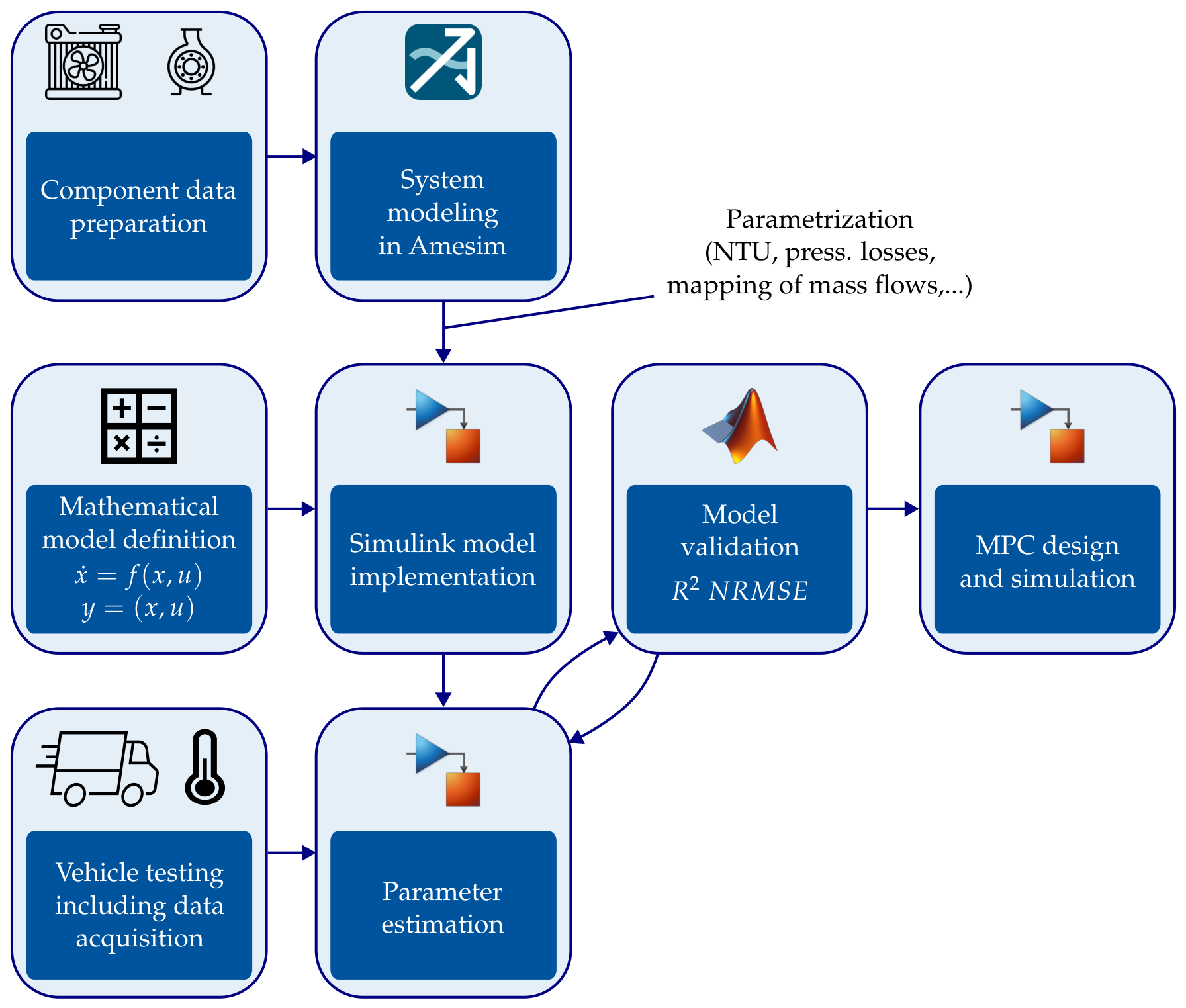
The methodology for NMPC development follows a structured, multi-stage process for controller development and validation. The individual development steps are illustrated in Figure 1.

The development begins with the preparation of manufacturer data for key thermal management system components. To efficiently parameterize these components using physics-based, high-fidelity models, a detailed thermal management system model is first developed in Simcenter Amesim, which provides validated component libraries and regression tools for heat-exchanger and pressure-loss characterization. Based on this model, essential system characteristics, such as the number of transfer units (NTU) and pressure losses, are extracted and transferred to a control-oriented Simulink model. Details on the Amesim modeling approach are provided in a previous publication [23].

In parallel, a mathematical representation of the system is formulated in nonlinear state-space form:

$$\dot{x}=f(x,u)$$

(1)

$$y=g(x,u)$$

(2)

where $x\in {\mathbb{R}}^n$ denotes the state vector, $u\in {\mathbb{R}}^m$ the control input, and $y\in {\mathbb{R}}^q$ the system output. The nonlinear vector fields $f(·)$ and $g(·)$ represent the thermodynamic energy balances, including flow-dependent heat-transfer coefficients derived from the NTU method as well as nonlinear couplings between mass flow rates and their associated temperature gradients.

This formulation provides the theoretical foundation for the nonlinear model predictive control (NMPC) design and simulation. The mathematical model is subsequently implemented and refined in a Simulink environment, where prediction accuracy is assessed through comparison with measurement data.

To ensure model accuracy, vehicle and test bench measurements are conducted and relevant data are collected. These empirical data are used within a Parameter Estimation Tool in MATLAB Simulink (version R2026a), where unknown or initially estimated parameters are adjusted to achieve agreement between the model and the measurement data. Following parameterization, the Simulink model is validated using standard statistical metrics for prediction accuracy.

The root mean square error (RMSE) is used to quantify the deviation between predicted and measured values. RMSE is defined as the square root of the mean of the squared differences between the predicted and observed values and is expressed as follows [24]:

$$RMSE=\sqrt{{\displaystyle \frac{1}{n}}\sum _{i=1}^n{(y_i-{\widehat{y}}_i)}^2}$$

(3)

where $y_i$ denotes the observed values, ${\widehat{y}}_i$ the predicted values, and n the number of data points.

Since RMSE is an absolute metric, a normalized RMSE (NRMSE) is used to improve comparability between different models. The NRMSE is defined here as

$$NRMSE={\displaystyle \frac{RMSE}{y_{max}-y_{min}}}$$

(4)

where $y_{max}$ and $y_{min}$ represent the maximum and minimum observed values per signal over the validation window, respectively.

In addition, the coefficient of determination $R^2$ is used as a further metric for evaluating model prediction accuracy. The value of $R^2$ indicates how well the model explains the variance of the observed data. It ranges from $-\infty$ to 1, where 1 represents a perfect prediction and values close to or below zero indicate poor model performance. The coefficient of determination is defined as follows [25]:

$$R^2=1-{\displaystyle \frac{{\sum }_{i=1}^n{(y_i-{\widehat{y}}_i)}^2}{{\sum }_{i=1}^n{(y_i-\overline{y})}^2}}$$

(5)

where $\overline{y}$ denotes the mean of the observed values. If the validation results are not satisfactory, the parameter estimation procedure is repeated.

Following successful validation, the validated model is used for NMPC design and subsequent simulation-based investigations. This structured approach ensures that the controller is developed on a physically realistic and experimentally substantiated basis, fulfilling both theoretical and practical requirements for thermal management systems in fuel-cell heavy-duty trucks.

3. Modeling of the Vehicle and Medium-Temperature Cooling Circuit

In this section, the modeling framework for the investigated heavy-duty fuel-cell vehicle and its medium-temperature cooling system is presented. First, the vehicle under study is described, followed by the development of a longitudinal vehicle dynamics model to capture the key driving and heat generation behaviors. The section then describes the thermal management system and the specific modeling of the medium-temperature cooling circuit. To support model accuracy, relevant test bench experiments and data collection procedures are presented, followed by a validation of the developed models. Finally, the selection of representative driving cycles and the implementation of the controller within the simulation environment are discussed, providing the foundation for subsequent simulation-based investigations.

3.1. Investigated Vehicle

The truck developed within the SeLv project is a fuel-cell electric truck specifically designed for long-haul heavy-duty applications. The vehicle is equipped with two hydrogen (${\mathrm{H}}_2$) storage tanks, with a system pressure of 350 bar and a total storage capacity of 35 $\mathrm{k}$$\mathrm{g}$. In addition to the ${\mathrm{H}}_2$ tanks, six battery packs with a total energy content of 368 $\mathrm{k}$$\mathrm{W}$$\mathrm{h}$ and a usable energy content of 300 $\mathrm{k}$$\mathrm{W}$$\mathrm{h}$, operating at a nominal voltage of 650 $\mathrm{V}$, serve as a central energy storage system for peak power demands and recuperated energy.

For energy conversion, two fuel-cell systems with a continuous electrical power of 85 $\mathrm{k}$$\mathrm{W}$ each and a system efficiency of approximately 50% are employed. The drivetrain consists of two mechanically coupled electric motors, where the output shaft of the first motor is directly connected to the input shaft of the second motor. This configuration enables flexible adjustment of the operating points of the electric machines: one motor can operate in traction mode, while the other simultaneously operates as a generator. This concept allows for operational optimization, load point shifting, and energy recuperation during vehicle operation.

The mechanical drive power is transmitted to the rear axle via a three-speed automated gearbox, enabling a continuous maximum power of 375 $\mathrm{k}$$\mathrm{W}$ at the wheel. A thermal management system designed for multiple temperature levels ensures effective heat dissipation from the battery, motors, power electronics, and fuel-cell system.

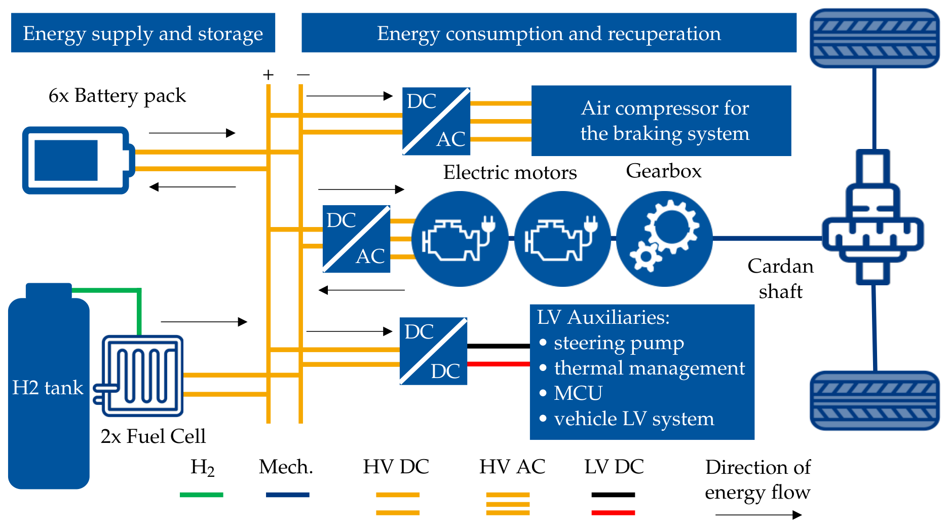
Figure 2 illustrates the drivetrain topology and the interaction of the main energy flows within the vehicle. Electrical energy is provided in direct current (DC) by the high-voltage battery and fuel-cell system, converted by inverters to supply the electric motors, and stepped down through DC/DC converters to power auxiliary systems, such as 24 $\mathrm{V}$ low-voltage units. The key technical specifications of the investigated vehicle are summarized in

Table 1. Technical specifications of the investigated vehicle.

Parameter	Value
Drivetrain power (30 min) †	375 $\mathrm{k}$$\mathrm{W}$
Peak drivetrain power †	468 $\mathrm{k}$$\mathrm{W}$
Gearbox	Three-speed automated
Fuel-cell power	$2\times 85 \mathrm{k}\mathrm{W}$
Peak fuel-cell power	$2\times 97 \mathrm{k}\mathrm{W}$
Battery energy content	300 $\mathrm{k}$$\mathrm{W}$$\mathrm{h}$
H2 storage capacity	35 $\mathrm{k}$$\mathrm{g}$, 350 bar

^† Continuous and peak mechanical power delivered at the wheel, combining both electric motors via the three-speed gearbox and final drive.

.

3.2. Longitudinal Vehicle Dynamics Model

To determine the drivetrain losses that represent the heat input for the thermal management models, the longitudinal dynamics of the vehicle are described using a backward calculation modeling approach. Prescribed driving cycles, defined by the vehicle speed and road gradient, are used as input. It is assumed that the vehicle perfectly follows the driving cycle, from which the required longitudinal driving resistance at the wheels, as well as the corresponding wheel speed and wheel torque, are calculated. From the wheel torque and the known overall gear ratio, operation points of motors with their corresponding losses can be determined.

A rule-based energy management strategy is employed to determine the fuel-cell power as a function of the battery state of charge (SoC). Lower SoC values result in higher requested fuel-cell power in order to maintain the battery SoC. This simplified strategy is sufficient for the generation of representative power losses and thermal loads.

The total longitudinal driving resistance at the wheels is modeled as the sum of rolling resistance, grade resistance, aerodynamic drag, and acceleration resistance [26]:

$$F_{\mathrm{total}}=F_{\mathrm{roll}}+F_{\mathrm{grade}}+F_{\mathrm{aero}}+F_{\mathrm{acc}}$$

(6)

The individual force components are calculated as

$$F_{\mathrm{roll}}=f_{\mathrm{roll}}·(m_{\mathrm{veh}}+m_{\mathrm{payload}})·g·cos\left({\alpha }_{\mathrm{grade}}\right)$$

(7)

$$F_{\mathrm{grade}}=(m_{\mathrm{veh}}+m_{\mathrm{payload}})·g·sin\left({\alpha }_{\mathrm{grade}}\right)$$

(8)

$$F_{\mathrm{aero}}=\frac{1}{2}·c_w·A·{\rho }_{\mathrm{air}}·v_{\mathrm{veh}}^2$$

(9)

$$F_{\mathrm{acc}}=(e_i·m_{\mathrm{veh}}+m_{\mathrm{payload}})·a_x$$

(10)

where $a_x$ is the longitudinal acceleration, $v_{\mathrm{veh}}$ the vehicle speed, ${\alpha }_{\mathrm{grade}}$ the road grade angle, $f_{\mathrm{roll}}$ the rolling resistance coefficient, $c_w$ the aerodynamic drag coefficient, A the vehicle frontal area, ${\rho }_{\mathrm{air}}$ the air density, and $e_i$ the rotational mass factor of the drivetrain.

The wheel rotational speed is calculated from the vehicle speed, while the wheel torque is obtained from the resulting total longitudinal force at the wheel. These relationships are given in Equations (11) and (12):

$$\begin{array}{cc}\hfill n_{\mathrm{wheel}}& ={\displaystyle \frac{60·v_{\mathrm{veh}}}{2\pi ·r_{\mathrm{dyn}}}}\hfill \end{array}$$

(11)

$$\begin{array}{cc}\hfill M_{\mathrm{wheel}}& =F_{\mathrm{total}}·r_{\mathrm{dyn}}\hfill \end{array}$$

(12)

Here, $n_{\mathrm{wheel}}$ denotes the wheel rotational speed in revolutions per minute and $M_{\mathrm{wheel}}$ the torque at the wheels. The parameter $r_{\mathrm{dyn}}$ represents the dynamic tyre radius, i.e., the effective rolling radius under load.

The parameters used in the longitudinal vehicle dynamics model are summarized in

Table 2. Parameters of the longitudinal vehicle dynamics model.

Parameter	Symbol	Value
Vehicle mass	$m_{\mathrm{veh}}$	11,000 kg
Payload	$m_{\mathrm{payload}}$	30,000 kg
Dynamic tire radius	$r_{\mathrm{dyn}}$	0.4923 m
Drag coefficient	$c_w$	0.583
Frontal area	A	9.9441  ${\mathrm{m}}^2$
Rolling resistance coefficient	$f_{\mathrm{roll}}$	0.0059
Mass factor	$e_i$	1.1
Air density	${\rho }_{\mathrm{air}}$	1.1839 $\mathrm{k}$$\mathrm{g}$ ${\mathrm{m}}^{-3}$

. The logic for gear shifting is implemented using a simple state machine, which is illustrated in Figure 3.

The simplified shift logic is based solely on the vehicle speed $v_{\mathrm{veh}}$ and models a three-speed transmission. The vehicle starts in first gear, with a total gear ratio of $i_{\mathrm{tot},1}=22.16$. When the vehicle speed exceeds 20 $\mathrm{k}\mathrm{m} {\mathrm{h}}^{-1}$, the transmission shifts to second gear, with a ratio of $i_{\mathrm{tot},2}=7.41$. At further speed increases ($v_{\mathrm{veh}}>50 \mathrm{k}\mathrm{m} {\mathrm{h}}^{-1}$), it shifts to third gear, with a ratio of $i_{\mathrm{tot},3}=2.467$. The third gear represents a direct drive, such that the total gear ratio corresponds to the axle drive ratio. Downshifting is also based on vehicle speed. If the vehicle speed falls below 45 $\mathrm{k}\mathrm{m} {\mathrm{h}}^{-1}$, the transmission shifts from third to second gear. If the speed further decreases below 15 $\mathrm{k}\mathrm{m} {\mathrm{h}}^{-1}$, it shifts back to first gear. The shift logic neglects additional variables such as torque demand or load request and therefore represents a heuristic shifting strategy.

The rotational speed of the electric machines is calculated from the wheel speed using the total gear ratio:

$$n_{\mathrm{M}}=n_{\mathrm{wheel}}·i_{\mathrm{tot}}$$

(13)

where $i_{\mathrm{tot}}$ denotes the total gear ratio of the selected gear, including gearbox and final drive.

If the torque at the wheels and the total gear ratio are known, the required torque of each electric machine can be determined. It is assumed that both machines share the wheel-torque demand equally. The required torque of a single machine is therefore calculated as

$$M_{\mathrm{M},\mathrm{req}}={\displaystyle \frac{0.5·M_{\mathrm{wheel}}}{i_{\mathrm{tot}}·{\eta }_{\mathrm{drivetrain}}}}$$

(14)

where $M_{\mathrm{M},\mathrm{req}}$ denotes the required torque of one electric machine and ${\eta }_{\mathrm{drivetrain}}$ represents the overall drivetrain efficiency, which is assumed to be constant and set to 0.93.

Efficiency and torque limitation maps of the electric machines are considered in the simulation. In drive mode (positive torque demand), the drive torque map specifies the maximum available machine torque $M_{\mathrm{M},\max }$ as a function of machine speed. The applied torque is limited accordingly. In generator mode (negative torque demand), a recuperation map defines the minimum achievable machine torque $M_{\mathrm{M},\min }$. If the braking power achievable by recuperation is exceeded, the remaining braking demand is covered by the mechanical braking system. The applied machine torque is described by

$$M_{\mathrm{M}}=\left\{\begin{array}{cc}min(M_{\mathrm{M},\mathrm{req}},M_{\mathrm{M},\max }),\hfill & M_{\mathrm{M},\mathrm{req}}>0\hfill \\ max(M_{\mathrm{M},\mathrm{req}},M_{\mathrm{M},\min }),\hfill & M_{\mathrm{M},\mathrm{req}}<0\hfill \end{array}\right.$$

(15)

where $M_{\mathrm{M},\max }$ and $M_{\mathrm{M},\min }$ represent the maximum and minimum available motor torque at the respective motor speed.

This approach ensures that the simulated machine torque always remains within the physically permissible limits of the drivetrain and that the transition between drive and generator operation is represented in a physically consistent manner.

It should be noted that while the described drivetrain architecture permits one motor to operate in traction and the other as a generator during certain maneuvers, this operating mode is not implemented in the vehicle or in the simulation conducted in this study. In both cases, the wheel-torque demand is distributed equally between the two motors at all times and both motors always operate in the same mode simultaneously, either both in traction or both in regeneration.

3.3. Thermal Management System

Following the modeling of the vehicle’s longitudinal dynamics and the resulting power demands, the associated thermal loads of the fuel-cell system and drivetrain components must be considered. In heavy-duty FCETs, these thermal interactions significantly influence efficiency, component durability, and operational limits, making the thermal management system a critical part of the overall vehicle architecture.

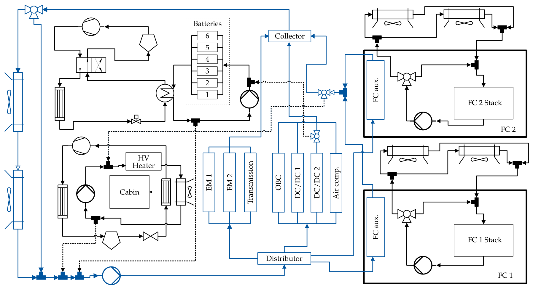
Figure 4 illustrates the complex thermal management system of the SeLv FCET, designed to ensure the reliable operation of all major components. The system includes two independent high-temperature cooling circuits, each dedicated to one of the two fuel-cell stacks. Each circuit operates at a coolant temperature of approximately 75 °C and includes two radiators connected in parallel, ensuring effective heat dissipation under high loads.

The MT circuit operates in a coolant temperature range of approximately 40 °C to 60 °C under the investigated operating conditions, distinguishing it from the high-temperature fuel-cell cooling circuits (75 °C) and the low-temperature battery circuit (20 °C).

For thermal protection of the batteries, a separate low-temperature (LT) cooling circuit is employed, maintained at a setpoint of approximately 20 °C. To keep the batteries within their optimal operating range even at high ambient temperatures, the water–glycol LT circuit is directly coupled to a vapor-compression refrigerant circuit via a plate heat exchanger (chiller), enabling active cooling.

Additionally, a separate refrigeration circuit manages cabin air conditioning and an independent heating circuit serves the purpose of heating the driver cabin. The MT, LT, and heating circuits can be interconnected via three-way valves, enabling flexible temperature management under varying operating conditions. This flexible design ensures maximum performance and longevity of all key components during vehicle operation.

3.4. Medium-Temperature Cooling Circuit Model

The medium-temperature cooling circuit is one of the key circuits within the thermal management system of the examined FCET. It is responsible for removing heat from the drivetrain, fuel-cell auxiliaries, electric motors, inverters, and other auxiliary consumers. In the simulation, a model of the MT cooling circuit was developed to capture the thermal behavior of the motors, inverters and fuel-cell auxiliaries. The DC/DC converters and the air compressor for the braking system are not included in this model, due to their negligible heat rejection.

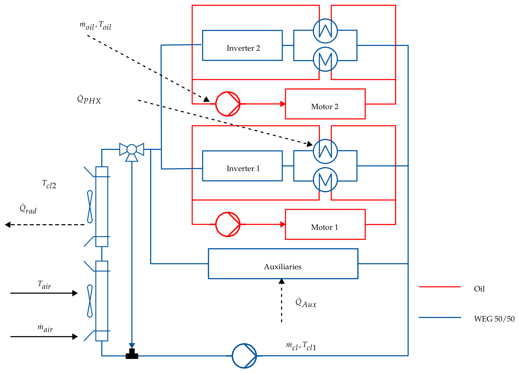
The structure of the MT cooling circuit model is shown in Figure 5. The circuit consists of the electric motors and auxiliary consumers, which act as the primary heat sources. Heat generated by the motors is transferred to the motor oil, which is circulated by an oil pump mechanically coupled to the motor shaft. The pump speed is assumed to be proportional to the motor speed.

The oil and coolant circuits are connected via four plate heat exchangers, with each of the two motors equipped with two heat exchangers. An electric pump circulates the coolant, while the motor oil is pumped by previously discussed mechanical pumps attached to the motor shafts. Heat is dissipated to the environment through two radiators, each equipped with two fans controlling the airflow.

In the model, the motors and auxiliary consumers are represented as lumped thermal masses to reduce the system order. The auxiliary consumers (motor inverters and fuel-cell auxiliaries) are modeled together as a single lumped mass, $m_{Aux}$. The heat-transfer coefficients and thermal resistances between lumped components are assumed to be constant, while heat transfer in the plate heat exchangers and radiators is captured using the NTU method with parameters calibrated from measurement data and the NTU regression tool in Simcenter Amesim. The lumped-parameter representation predicts bulk component temperatures relevant to cooling actuation and does not resolve local temperature gradients.

The dominant thermal time constant of the motor-to-oil cooling path, computed from the identified mass, specific heat, and thermal resistance $(m_M·c_{p,M})/(2/R_{th,M,oil})$, is approximately 192 $\mathrm{s}$. In the SeLv driving cycle used for controller evaluation, 95% of acceleration events last 24 s or less and the single longest acceleration phase across the entire $9.7$ $\mathrm{h}$ cycle lasts 56 $\mathrm{s}$, both substantially shorter than the dominant thermal time constant. Acceleration-induced heat-generation transients are therefore strongly damped at the bulk-temperature level, supporting the model’s applicability for the control-relevant dynamics investigated in this work, even though it does not resolve instantaneous local hot-spot formation. Sustained high-load conditions, such as prolonged uphill driving, differ fundamentally from acceleration transients, in that the elevated heat generation persists for a duration comparable to or exceeding the relevant thermal time constants rather than being damped by thermal inertia. This operating regime is nevertheless addressed by the experimental validation: the test bench measurements (Section 3.7) include a sustained full-load segment corresponding to the continuous power output test prescribed by UN/ECE Regulation No. 85, lasting 30 $\min$. Analysis of the slope profile of the SeLv driving cycle shows that, even for a conservative sustained-grade threshold of 2%, the longest continuous uphill segment across the entire $9.7$ $\mathrm{h}$ cycle lasts approximately 310 $\mathrm{s}$ ($5.2$ $\min$), with a mean grade of 5.8% and a maximum of 7.9%. Since the validated sustained full-load segment exceeds this duration by close to a factor of six, and the developed model accurately reproduces the measured temperature evolution under that sustained high-load condition (Section 3.9), the validated applicability of the model extends to thermally comparable scenarios, such as extended climbing, since the cooling system’s response depends on the magnitude and duration of the resulting heat generation rather than on whether it originates from vehicle speed, payload, or road grade.

The differential Equations (16)–(20) describe the thermal behavior of the cooling system. Nomenclature used in the model is listed in

Table 3. Nomenclature used in the medium-temperature cooling circuit model.

Quantity	Symbol/Unit
Specific heat capacity of component x	$c_{p,x}$/$\mathrm{J} {\mathrm{kg}}^{-1} {\mathrm{K}}^{-1}$
Mass of component x	$m_x$/$\mathrm{k}\mathrm{g}$
Temperature of component x	$T_x$/$\mathrm{K}$
Thermal resistance between components x and y	$R_{\mathrm{th},x,y}$/$\mathrm{K} {\mathrm{W}}^{-1}$
Heat-flow rate at component x	${\dot{Q}}_x$/$\mathrm{W}$
Heat-transfer coefficient between components x and y	${\alpha }_{x,y}$/$\mathrm{W} {\mathrm{m}}^{-2} {\mathrm{K}}^{-1}$

.

Equation (16) describes the energy balance of the two electric motors in the cooling system model. The factor of 2 in the second and third terms accounts for the presence of two identical motors.

$$m_{\mathrm{M}}·c_{\mathrm{p},\mathrm{M}}·{\displaystyle \frac{d{T}_{\mathrm{M}}}{dt}}=2·{\dot{Q}}_{\mathrm{loss},\mathrm{M}}-2·{\displaystyle \frac{T_{\mathrm{M}}-T_{\mathrm{oil}}}{R_{\mathrm{th},\mathrm{M},\mathrm{oil}}}}-2·{\alpha }_{\mathrm{M},\mathrm{air}}·A_{\mathrm{M}}·(T_{\mathrm{M}}-T_{\mathrm{amb}})$$

(16)

Here, $m_M$ denotes the combined thermal mass of both motor units, and all heat-flow terms in Equation (16) represent the aggregated contributions of both motors, consistent with the parallel operation and equal torque distribution described in Section 3.2. The term ${\alpha }_{M,\mathrm{air}}·A_M·(T_{\mathrm{M}}-T_{\mathrm{amb}})$ represents direct convective heat dissipation from the motor housing to the ambient air, with ${\alpha }_{\mathrm{M},\mathrm{air}}$ denoting the motor-to-air heat-transfer coefficient and $A_M$ the effective surface area. Equation (17) describes the energy balance of the motor oil:

$$m_{\mathrm{oil}}·c_{\mathrm{p},\mathrm{oil}}·{\displaystyle \frac{d{T}_{\mathrm{oil}}}{dt}}=2·{\displaystyle \frac{T_{\mathrm{M}}-T_{\mathrm{oil}}}{R_{\mathrm{th},\mathrm{M},\mathrm{oil}}}}-4·{\dot{Q}}_{\mathrm{PHX}}$$

(17)

Equation (18) describes the energy balance of the auxiliary consumers:

$$m_{\mathrm{aux}}·c_{p,\mathrm{aux}}·{\displaystyle \frac{d{T}_{\mathrm{aux}}}{dt}}={\dot{Q}}_{\mathrm{loss},\mathrm{aux}}-{\displaystyle \frac{T_{\mathrm{aux}}-T_{\mathrm{c}\mathrm{l}1}}{R_{\mathrm{th},\mathrm{aux},\mathrm{cl}}}}$$

(18)

The coolant in the channels outside the radiator is modeled as a lumped mass, simplifying the thermal dynamics. The corresponding energy balance is given by Equation (19):

$$m_{\mathrm{c}\mathrm{l}1}·c_{p,\mathrm{cl}}·{\displaystyle \frac{d{T}_{\mathrm{c}\mathrm{l}1}}{dt}}=4·{\dot{Q}}_{\mathrm{PHX}}-{\dot{m}}_{\mathrm{cl}}·c_{p,\mathrm{cl}}·(T_{\mathrm{c}\mathrm{l}1}-T_{\mathrm{c}\mathrm{l}2})+{\displaystyle \frac{T_{\mathrm{aux}}-T_{\mathrm{c}\mathrm{l}1}}{R_{\mathrm{th},\mathrm{aux},\mathrm{cl}}}}$$

(19)

Similarly, the coolant in the radiator is modeled as a lumped mass, with its energy balance given by Equation (20):

$$m_{\mathrm{c}\mathrm{l}2}·c_{p,\mathrm{cl}}·{\displaystyle \frac{d{T}_{\mathrm{c}\mathrm{l}2}}{dt}}={\dot{m}}_{\mathrm{cl}}·c_{p,\mathrm{cl}}·(T_{\mathrm{c}\mathrm{l}1}-T_{\mathrm{c}\mathrm{l}2})-{\dot{Q}}_{\mathrm{rad}}$$

(20)

These differential equations form the state-space representation of the MT cooling circuit and are used in the vehicle simulation to predict component temperatures under varying operating conditions.

The heat-transfer coefficient ${\alpha }_{M,air}$, together with the heat-resistance coefficients for the remaining lumped thermal masses, are treated as constant parameters identified from test bench measurement data using the Simulink Parameter Estimation Tool (Section 3.8). This assumption of constant heat-transfer coefficients is a deliberate modeling simplification for the lumped component masses, where the dominant uncertainty lies in the effective thermal resistance between components rather than in flow-dependent convective effects. This should be distinguished from the heat-exchanger sub-models (Equations (22) and (26)), where heat-transfer effectiveness is explicitly flow-dependent through NTU correlations that account for Reynolds-number-dependent convection on both the coolant and air sides. The assumption of constant heat-transfer coefficients for the lumped masses is validated implicitly by the model accuracy reported in Section 3.9.

The heat exchanged in the plate heat exchanger (PHX) is calculated using the $\epsilon$–NTU method. This approach has been applied in previous work by the authors [23,27] and is also described in standard heat-transfer textbooks, such as [28]. The heat-flow rate transferred in the plate heat exchanger is given by

$${\dot{Q}}_{\mathrm{PHX}}={\epsilon }_{\mathrm{PHX}}·C_{\min ,\mathrm{PHX}}·(T_{\mathrm{oil}}-T_{\mathrm{c}\mathrm{l}1})$$

(21)

The heat-exchanger effectiveness is calculated using the formulation for counterflow heat exchangers, as oil and coolant flow in opposite directions [29]. Accordingly, the effectiveness of the plate heat exchanger is expressed as

$${\epsilon }_{\mathrm{PHX}}={\displaystyle \frac{1-exp(-\mathrm{NTU}(1-C_r))}{1-C_r·exp(-\mathrm{NTU}(1-C_r))}}$$

(22)

where $C_r=C_{\min }/C_{\max }$ represents the ratio of the minimum heat capacity rate to the maximum heat capacity rate ($C=\dot{m}·c_p$). The oil pumps are mechanically coupled to the electric motors. At a motor speed of 3500 ${\min }^{-1}$, the volumetric flow rate of motor oil is 60 $\mathrm{L}$ ${\min }^{-1}$. A linear relationship between motor speed and oil volume flow is assumed, while the oil density is considered constant. Based on these assumptions, the mass flow rate of motor oil is calculated as

$${\dot{m}}_{\mathrm{oil}}={\displaystyle \frac{60}{3500}}·n_{\mathrm{Motor}}·{\displaystyle \frac{1}{\mathrm{60,000}}}·{\rho }_{\mathrm{oil}}$$

(23)

The specific heat capacity of the motor oil in $\mathrm{J} {\mathrm{kg}}^{-1} {\mathrm{K}}^{-1}$ is approximated by a linear function of the oil temperature. Correlations for the calculation of fluid properties are presented in

Table A3. Fluid thermal property correlations (temperature T in °C).

Property	Correlation	Unit
$c_{p,\mathrm{oil}}\left(T_{\mathrm{oil}}\right)$	$4.2857·T_{\mathrm{oil}}+1864$	J/(kg K)
${\rho }_{\mathrm{oil}}$	848 (constant)	kg/m3
$c_{p,\mathrm{cl}}\left(T_{\mathrm{cl}}\right)$	$0.043·T_{\mathrm{cl}}+3.2254$	kJ/(kg K)
${\rho }_{\mathrm{cl}}\left(T_{\mathrm{cl}}\right)$	$-0.6154·T_{\mathrm{cl}}+1072.6$	kg/m3

.

Heat transfer in the radiator depends on the ambient air mass flow rate, the coolant mass flow rate, the ambient air temperature, and the coolant temperature at the radiator inlet (point 2). In general form, the radiator heat-flow rate can be expressed as

$${\dot{Q}}_{\mathrm{rad}}=f({\dot{m}}_{\mathrm{air}},{\dot{m}}_{\mathrm{cl}},T_{\mathrm{amb}},T_{\mathrm{c}\mathrm{l}2})$$

(24)

Using the $\epsilon$–NTU method, the heat transfer in the radiator is calculated as

$${\dot{Q}}_{\mathrm{rad}}={\epsilon }_{\mathrm{rad}}·C_{\min ,\mathrm{rad}}·\left(T_{\mathrm{c}\mathrm{l}2}-T_{\mathrm{amb}}\right)$$

(25)

The effectiveness of the radiator is calculated according to the formula for cross-flow heat exchangers with both fluids unmixed [28]:

$${\epsilon }_{\mathrm{rad}}=1-exp\left({\displaystyle \frac{1}{C_r}}{\left(NTU\right)}^{0.22}\left[exp\left(-C_r{\left(NTU\right)}^{0.78}\right)-1\right]\right)$$

(26)

The ambient air mass flow through the radiator package was derived from CFD simulations of the complete truck model, including integrated representations of the components located in the former engine compartment, where fuel cells and auxiliaries are now installed. The CFD analyses were performed at 100% fan speed and the resulting airflow data were used to identify the system resistance characteristic of the cooling package.

The fan behavior was described using the manufacturer’s pressure–flow characteristic map and scaled to partial rotational speeds by applying the fan affinity laws. Parallel fan operation was modeled by representing the fans as an equivalent single fan with an increased flow capacity. The pressure losses of the cooling system were modeled as a quadratic function of the air mass flow, complemented by a ram pressure term derived from the vehicle’s dynamic pressure. The system constant was obtained from the CFD operating points and the operating condition for arbitrary fan speeds and vehicle velocities was determined from the intersection of the fan characteristic and the system resistance curve.

The characterization of the plate heat exchangers, radiator, and cooling fans relies on a combination of manufacturer data, CFD simulations, and test bench measurements, each contributing to a different stage or aspect of the model rather than being merged through a single fusion step. For the plate heat exchangers and radiator, the heat-transfer effectiveness ((Equations (22) and (26)) is determined in two sequential steps: manufacturer-supplied heat-exchanger performance data is first processed using the regression tool in Simcenter Amesim to obtain an initial parameterized correlation consistent with the underlying heat-transfer physics; these parameters are then re-estimated using drivetrain test bench measurement data and the Simulink Parameter Estimation Tool, such that the final reported values reflect calibration against the measured system behavior rather than the manufacturer data alone. This sequential procedure, rather than weighted averaging or piecewise fitting, is used to combine the two data sources: the manufacturer-derived correlation provides a physically grounded starting point and functional form, while the test bench-based re-estimation corrects for deviations arising from installation effects, manufacturing tolerances, and other system-level influences not captured by component-level manufacturer data. The air-side system resistance of the radiator package, which determines the relationship between air mass flow rate and fan speed (Equation (33)), is derived independently from CFD simulations of the complete vehicle, performed at full fan speed. The fan pressure–flow characteristic itself is taken from manufacturer specifications and scaled to partial rotational speeds using the fan affinity laws; this sub-model is informed by manufacturer data only.

Differences in reliability between these data sources, such as manufacturer tolerance bands, CFD turbulence, and meshing assumptions and the limited operating envelope of the test bench measurements, introduce uncertainty into the respective sub-models. However, since the heat-transfer parameters that most directly determine predicted component temperatures are calibrated end-to-end against measured data, uncertainty originating from the CFD-derived air-side resistance or the manufacturer’s fan characteristic is implicitly compensated for during this calibration step. The reported validation metrics (${\mathrm{R}}^2$ > 0.9, NRMSE < 10%, Section 3.9) therefore reflect the net predictive accuracy of the model after calibration rather than an unconstrained propagation of upstream uncertainty. A formal uncertainty propagation analysis across the individual data sources, such as a sensitivity study over CFD and manufacturer input variability, was not performed, and this is identified as a direction for future work.

3.5. Actuator Power Consumption Models

The auxiliary energy consumption of the cooling system, which constitutes the primary optimization objective of the NMPC, is computed by integrating the electrical power demand of the coolant pump and the radiator fans over the simulation horizon.

The electrical power of the coolant pump is determined from the product of terminal voltage and current, $P_{\mathrm{pump}}=U_{\mathrm{pump}}·I_{\mathrm{pump}}$. The terminal voltage is assumed to be approximately constant at its measured mean value during operation. The current is modeled as a third-order polynomial function of pump speed, fitted to discrete current measurements at multiple operating points, with a coefficient of determination of $R^2=0.9988$. The exact polynomial coefficients are subject to a non-disclosure agreement and are not reproduced here. Within the NMPC operating range of 1400–5600 rpm, the resulting pump power ranges from approximately 270 $\mathrm{W}$ to 1820 $\mathrm{W}$. The total pump energy consumption is obtained by time integration of $P_{\mathrm{pump}}$:

$$E_{\mathrm{pump}}={\displaystyle \frac{1}{3.6\times {10}^6}}\int P_{\mathrm{pump}}\left(t\right)\mathrm{d}t\left[\mathrm{kWh}\right]$$

(27)

The electrical power of a single fan set (comprising two fans) is modeled as a third-order polynomial function of fan speed, fitted to discrete power measurements, with a coefficient of determination of $R^2=0.9987$:

$$P_{\mathrm{fan},\mathrm{s}}=4\times {10}^{-4}·{\tilde{n}}_{\mathrm{fan}}^3-1.04\times {10}^{-2}·{\tilde{n}}_{\mathrm{fan}}^2+7.91\times {10}^{-1}·{\tilde{n}}_{\mathrm{fan}}\left[\mathrm{W}\right]$$

(28)

where ${\tilde{n}}_{\mathrm{fan}}$ denotes the fan speed expressed as a percentage of the maximum rated speed (2570 rpm), i.e., ${\tilde{n}}_{\mathrm{fan}}=n_{\mathrm{fan}}·100/2570$. The total fan power of both fan sets is

$$P_{\mathrm{fan}}=2·P_{\mathrm{fan},\mathrm{s}}$$

(29)

and the corresponding energy consumption is

$$E_{\mathrm{fan}}={\displaystyle \frac{1}{3.6\times {10}^6}}\int P_{\mathrm{fan}}\left(t\right)\mathrm{d}t\left[\mathrm{kWh}\right]$$

(30)

The total auxiliary cooling energy, reported in Section 4, is $E_{\mathrm{CS}}=E_{\mathrm{pump}}+E_{\mathrm{fan}}$.

3.6. Heat Source Modeling

The heat generation terms ${\dot{Q}}_{\mathrm{loss},\mathrm{M}}$ and ${\dot{Q}}_{\mathrm{loss},\mathrm{aux}}$ are computed from manufacturer-supplied component data as described below.

The motor heat generation ${\dot{Q}}_{\mathrm{loss},\mathrm{M}}$ is determined from a two-dimensional lookup table with motor speed $n_{\mathrm{M}}$ and motor torque $M_{\mathrm{M}}$ as inputs, derived from the manufacturer-supplied efficiency map ${\eta }_{\mathrm{M}}(n_{\mathrm{M}},M_{\mathrm{M}})$. The lookup table output represents the heat dissipated per motor as a function of the current operating point; since both motors are operated in parallel with equal torque distribution at all times (Section 3.2), the total motor heat generation is obtained by multiplying the per-motor loss by a factor of two, as reflected in the first term on the right-hand side of Equation (16). The exact efficiency map data are subject to a non-disclosure agreement and cannot be reproduced here.

The aggregated auxiliary heat load ${\dot{Q}}_{\mathrm{loss},\mathrm{aux}}$ comprises contributions from three sources. First, the SiC inverter losses are determined from a two-dimensional lookup table with the same inputs ($n_{\mathrm{M}}$, $M_{\mathrm{M}}$) as the motor loss map, again derived from manufacturer data and multiplied by two to account for both inverters. Second, the fuel-cell auxiliary heat rejection is determined from a one-dimensional lookup table linking the fuel-cell net electrical power to the rejected heat per fuel cell; this heat rejection ranges from 0 $\mathrm{k}$$\mathrm{W}$ at zero power to $7.6$ $\mathrm{k}$$\mathrm{W}$ at the maximum considered fuel-cell power of 80 $\mathrm{k}$$\mathrm{W}$ per unit and is multiplied by two to account for both fuel-cell units.

Third, heat contributions from the remaining auxiliary components (coolant pumps, fans, and control electronics) were measured during the test bench campaign and found to amount to at most a few hundred watts in total; these contributions are considered negligible relative to the dominant heat sources and are excluded from the model. The three contributions are summed to yield ${\dot{Q}}_{\mathrm{loss},\mathrm{aux}}$, which serves as a disturbance input to the auxiliary thermal mass state equation (Equation (18)).

3.7. Test Bench Experiments and Data Collection

As part of the SeLv project, test bench experiments were conducted on the roller dynamometer at DLG TestService GmbH in Groß-Umstadt, Germany. The primary objective of these tests was to perform homologation measurements of the fuel-cell truck, as documented in the corresponding DLG press release [30].

The test bench is equipped with two driven roller axles and enables the execution of standardized driving cycles under highly reproducible conditions. The test chamber is climate-controlled and allows ambient temperatures of up to 45 °C. Conditioned airflow is supplied to the vehicle via an air inlet system to emulate the cooling airflow encountered during real driving operation. In addition, the rear-axle differential was actively cooled by a dedicated fan to prevent overheating during sustained high-load operation. These conditions allow the reproduction of long-duration load cycles and worst-case operating scenarios with high repeatability and well-defined boundary conditions.

The experiments focused on evaluating several key aspects of the heavy-duty fuel-cell truck. First, drivetrain performance and braking behavior were assessed under various operating conditions, including continuous load operation and recuperation phases. Second, the TMS was investigated with respect to heat dissipation capability and thermal stability under full-load operation and ambient temperatures of up to 40 °C, representing extreme summer conditions. Finally, tests were conducted to fulfill homologation requirements and obtain operating permits in accordance with UN/ECE Regulation No. 13, addressing continuous braking and recuperation and UN/ECE Regulation No. 85, specifying continuous power output over a duration of 30 $\min$. The measurement data acquired during the TMS tests were subsequently used for the calibration and validation of the simulation models presented in this work. The selected operating point represents a critical high-thermal-load condition (ambient temperature of 40 °C, full-load operation), which is considered representative for thermal validation in heavy-duty applications.

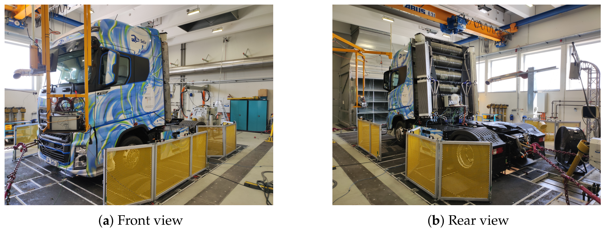
Figure 6 provides an overview of the test bench setup. The first subfigure presents the front view of the vehicle, where the driver display used for monitoring relevant vehicle data during the test is shown. The second subfigure shows the rear view of the vehicle, illustrating the chain-based vehicle fastening system and the large axial fan used for active cooling of the rear-axle differential. Behind the vehicle’s hydrogen tanks, a housing containing the data acquisition system is visible, comprising a modular Q.brixx measurement system from Gantner Instruments Test Measurement GmbH in Lauf an der Pegnitz, Germany.

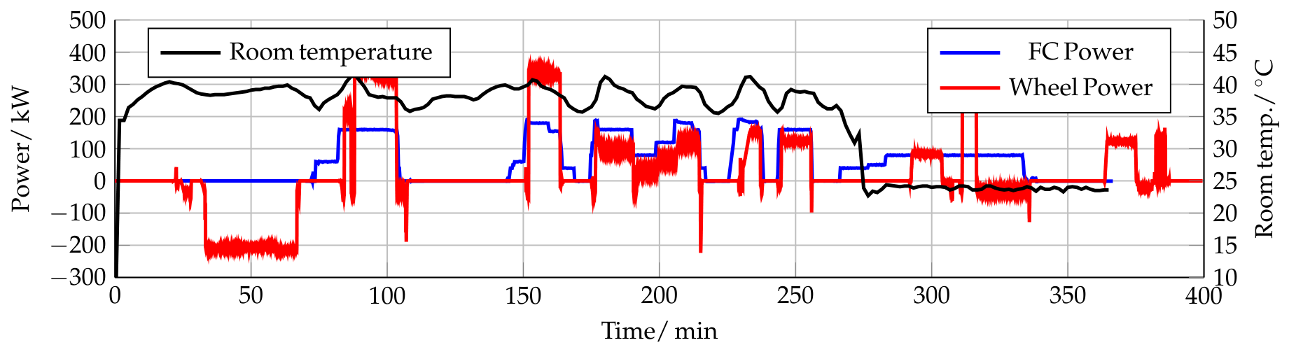
The conducted tests covered a wide range of power levels, whose variations over time are illustrated in Figure 7. Although the primary purpose of these tests was homologation, the recorded data proved well suited for validating the simulation models developed in this work.

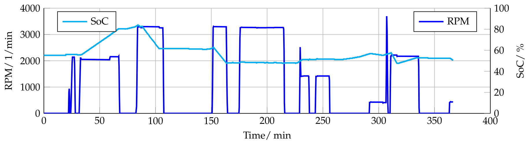
Figure 8 shows the behavior of the SoC and the motors’ RPM during the same experiment.

3.8. Parameter Identification Setup

The uncertain model parameters were identified using the Simulink Parameter Estimation Tool with a nonlinear least-squares objective function minimizing the sum of squared residuals between simulated and measured temperatures across all monitored channels simultaneously, with equal weighting applied to all channels. The Trust-Region-Reflective algorithm was used with a parameter tolerance of ${10}^{-3}$, a function tolerance of ${10}^{-3}$, and a maximum of 100 iterations. Measurement data were used at the original 1 $\mathrm{Hz}$ sampling rate without filtering or preprocessing.

The parameters subject to estimation, together with their initial values and search bounds, are listed in

Table 4. Parameters estimated using the Simulink Parameter Estimation Tool, with initial values and search bounds. Final values are reported in Appendix A.

Symbol	Description	Initial Value	Min	Max
${\alpha }_{M,\mathrm{air}}$	Motor-to-air heat-transfer coefficient [W/(m2 K)]	58.49	0	200
$m_{\mathrm{oil}}$	Oil mass [kg]	4.920	1	50
$R_{\mathrm{th},\mathrm{M},\mathrm{oil}}$	Motor-to-oil thermal resistance [K/W]	$4.77\times {10}^{-4}$	0	1
$R_{\mathrm{th},\mathrm{aux},\mathrm{cl}}$	Auxiliary-to-coolant thermal resistance [K/W]	$2.14\times {10}^{-3}$	0	1
$a_{1,\mathrm{PHX}}$	PHX oil-side heat-transfer coefficient [–]	9,127,950	0	∞
$b_{1,\mathrm{PHX}}$	PHX oil-side flow exponent [–]	4.962	0	10
$a_{2,\mathrm{PHX}}$	PHX coolant-side heat-transfer coefficient [–]	1189.91	0	∞
$b_{2,\mathrm{PHX}}$	PHX coolant-side flow exponent [–]	1.172	0	10
$a_{1,\mathrm{RAD}}$	Air-side Nusselt coefficient [–]	0.02306	0	5
$b_{1,\mathrm{RAD}}$	Air-side Nusselt exponent [–]	0.6896	0	10
$a_{2,\mathrm{RAD}}$	Coolant-side Nusselt coefficient [–]	0.7061	0	10
$b_{2,\mathrm{RAD}}$	Coolant-side Nusselt exponent [–]	0.9944	0	10

. Initial values for the plate heat-exchanger coefficients $a_{1,\mathrm{PHX}}$ and $a_{2,\mathrm{PHX}}$ and the radiator Nusselt coefficients were taken from the Amesim regression described in Section 3.4; initial values for the thermal masses and resistances were derived from physical reasoning and manufacturer-supplied material data. The remaining model parameters, including the wall thermal conductances $G_{\mathrm{wall},\mathrm{PHX}}$ and $G_{\mathrm{wall},\mathrm{RAD}}$, all geometric constants, and the fluid property correlations, were held fixed at the values reported in Appendix A. The final identified parameter values are also reported in Appendix A.

3.9. Model Validation

This section utilizes the measurement data obtained from the test bench experiments described in Section 3.7 to validate the developed simulation models. The objective is to establish a validated model that accurately represents the real-system behavior and can subsequently be used for the development and evaluation of a model predictive control strategy.

The experimental data were supplied to the Simulink Parameter Estimation Tool (as explained in Section 3.8) in order to identify model parameters subject to uncertainty during the modeling process. The parameter estimation was performed with the aim of achieving a high level of agreement between simulation and measurement, quantified by the coefficient of determination ${\mathrm{R}}^2$ and the normalized root mean square error (NRMSE).

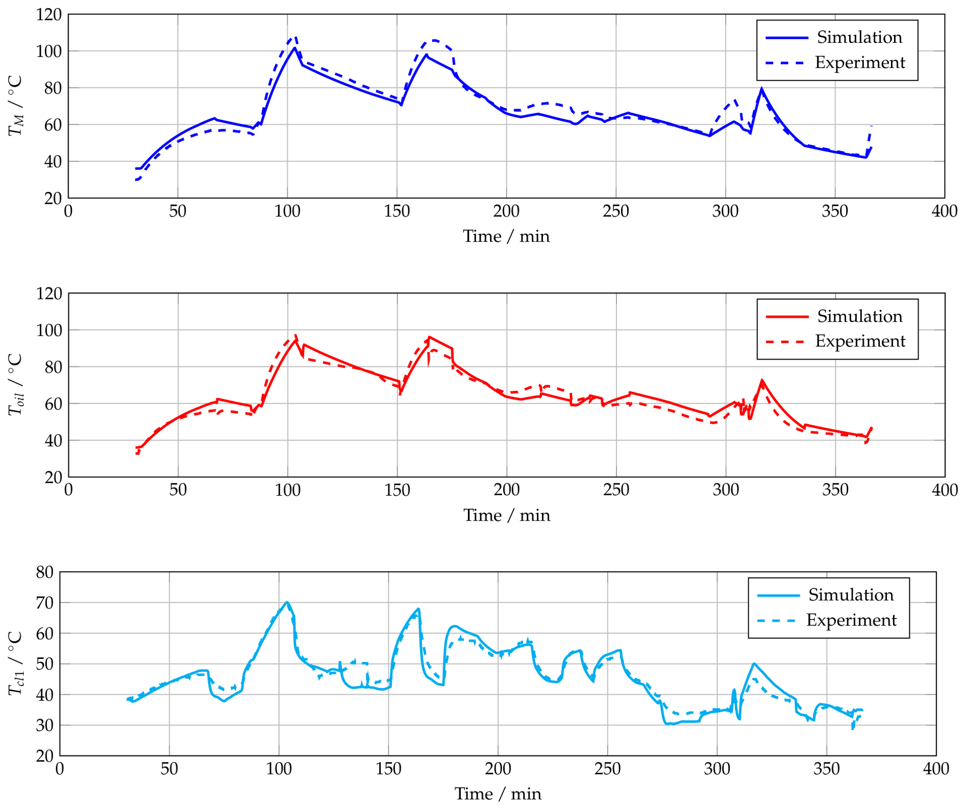
The validation results for the motor winding, oil, and coolant temperatures are shown in Figure 9. The target criteria of ${\mathrm{R}}^2>0.9$ and NRMSE $<10\%$ were achieved for all three temperatures, as summarized in

Table 5. Evaluation metrics quantifying the deviation between simulated and measured temperatures of coolant ($T_{cl1}$), motor windings ($T_M$), and oil ($T_{oil}$).

Variable	${\mathbf{R}}^2$ (-)	RMSE	NRMSE (%)
$T_{cl1}$	0.91	$2.60$  $°\mathrm{C}$	6.19
$T_M$	0.93	$4.54$  $°\mathrm{C}$	5.75
$T_{oil}$	0.93	$3.88$  $°\mathrm{C}$	6.03

. For the coolant temperature, the resulting root mean square error of $\mathrm{RMSE}=2.6 °\mathrm{C}$ is smaller than the specified sensor accuracy of $\pm 3.29 °\mathrm{C}$ within the relevant measurement range of 20 °C to 120 °C, as stated in the manufacturer datasheet for the temperature sensors used on the test bench. This suggests that the remaining model deviation is of the same order of magnitude as the measurement uncertainty, though a formal uncertainty propagation analysis was not performed. For the motor winding and oil temperatures, the RMSE values of $4.54 °\mathrm{C}$ and $3.88 °\mathrm{C}$, respectively, slightly exceed the nominal sensor accuracy, which is acknowledged as a limitation of the current model parameterization. They remain within an acceptable range for thermal management applications, particularly in light of the high coefficients of determination and low NRMSE values. Overall, the obtained validation metrics demonstrate that the model reproduces the measured thermal dynamics with sufficient accuracy for subsequent NMPC design and analysis.

The model was identified using data up to 280 min at approximately 40 °C ambient temperature and subsequently validated against the remaining measurement period, during which ambient temperature decreased to approximately 25 °C. The model accurately reproduces thermal behavior across this temperature range without re-identification. It should be noted, however, that both periods were recorded within a single continuous test campaign using a temporal holdout approach rather than validation against an independent experiment or driving profile; the reported accuracy metrics therefore characterize the model’s ability to reproduce the measured thermal dynamics within the validated test campaign and operating conditions described below.

While the resulting ambient temperature span (approximately 25 °C to 40 °C) covers a meaningful portion of the conditions relevant to heavy-duty operation in temperate and warm climates, other aspects of the broader operating envelope were not part of this dedicated thermal validation campaign. Reduced air density at higher altitude would be expected to lower radiator convective effectiveness and fan power demand, an effect not captured by the current calibration. Ambient humidity is considered to have limited direct relevance to the medium-temperature circuit investigated here, since heat rejection in this circuit occurs through the oil and coolant circuits rather than through processes directly sensitive to air humidity, such as fuel-cell stack hydration or cabin air conditioning.

Validation data at sub-zero ambient temperatures was not available, as the climate-controlled roller test bench used for the homologation campaign (Section 3.7) does not support sub-zero ambient conditions and dedicated low-temperature testing was outside the scope of the available test campaign. At lower ambient temperatures, several effects not captured by the current calibration would be expected to become relevant: the temperature-dependent specific-heat correlation for the motor oil (Table A3) was identified within the oil temperature range observed during this test and would require extrapolation outside it; oil viscosity increases at low temperature would alter pump losses and could affect the assumed proportionality between motor speed and oil mass flow (Equation (23)); and the NTU-based heat-exchanger correlations were calibrated from, and only verified within, the observed ambient range. Quantifying these effects would require dedicated low-temperature testing and this is identified as a direction for future work.

Of the five model states, direct sensor measurements were available for $T_{\mathrm{c}\mathrm{l}1}$, $T_M$, and $T_{\mathrm{oil}}$ during the test campaign and validation was performed against these three channels. Direct validation of $T_{\mathrm{aux}}$ is not possible, as this state represents a lumped equivalent thermal mass aggregating multiple heterogeneous auxiliary components rather than a single physically measurable temperature; individual component temperature measurements available from the test bench reflect local operating conditions rather than the aggregated bulk state that $T_{\mathrm{aux}}$ models. The thermal influence of $T_{\mathrm{aux}}$ on the validated state $T_{\mathrm{c}\mathrm{l}1}$ is implicitly captured through the identified heat-transfer resistance $R_{\mathrm{th},\mathrm{aux},\mathrm{cl}}$. Direct validation of $T_{\mathrm{c}\mathrm{l}2}$ was not performed as no sensor was installed at the radiator coolant inlet during the test campaign; the available measurements reflect local outlet temperatures of individual circuit components rather than the flow-weighted mixture temperature at the radiator inlet that $T_{\mathrm{c}\mathrm{l}2}$ models. Since $T_{\mathrm{c}\mathrm{l}2}$ is algebraically coupled to $T_{\mathrm{c}\mathrm{l}1}$ through the coolant energy balance, a model that accurately tracks $T_{\mathrm{c}\mathrm{l}1}$ and correctly reproduces the radiator heat rejection implicitly constrains $T_{\mathrm{c}\mathrm{l}2}$ within physically consistent bounds.

3.10. Driving Cycle Selection

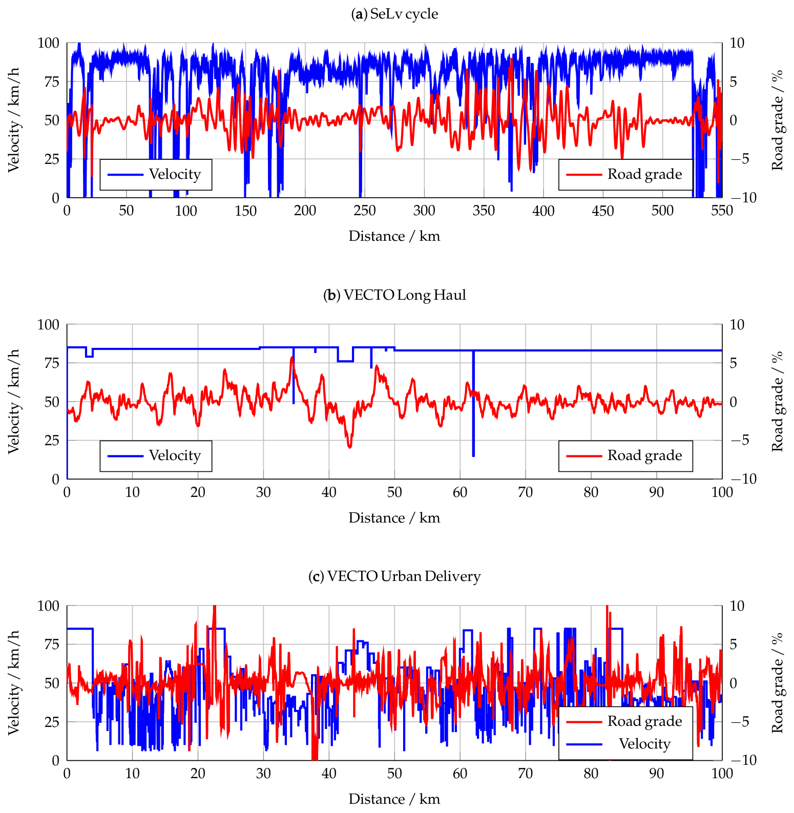
To evaluate the controller performance under realistic driving conditions, three representative driving cycles are considered, as shown in Figure 10. The first cycle was recorded within the SeLv project on a route in western Germany comprising both highway and rural road sections. Further details on this cycle are provided in [31] and its speed profile is depicted in Figure 10a.

To investigate the controller behavior under conditions dominated by sustained highway driving with minimal stop phases, the VECTO Long Haul cycle was selected, as shown in Figure 10b. In contrast, the VECTO Urban Delivery cycle was chosen to assess controller performance under frequent speed changes and transient operating conditions, as illustrated in Figure 10c. VECTO is a simulation framework developed by the European Commission for the determination of CO₂ emissions and fuel consumption of heavy-duty vehicles [32].

3.11. Controller Implementation in Simulation

This section presents the NMPC strategy developed for the thermal management of the MT cooling circuit. For implementation in MATLAB/Simulink, the optimization problem is formulated based on a control-oriented state-space representation of the system dynamics.

The NMPC model comprises five states $\mathbf{x}$, seven inputs $\mathbf{u}$, and five outputs $\mathbf{y}$. The states represent the temperatures of the main thermal components of the MT cooling circuit. The states and inputs are summarized in (31).

$$\begin{array}{c}\hfill \mathbf{x}=\left[\begin{array}{c}{x}_1\\ x_2\\ x_3\\ x_4\\ x_5\end{array}\right]=\left[\begin{array}{c}{T}_M\\ T_{oil}\\ T_{aux}\\ T_{cl1}\\ T_{cl2}\end{array}\right],\mathbf{u}=\left[\begin{array}{c}{u}_1\\ u_2\\ u_3\\ u_4\\ u_5\\ u_6\\ u_7\end{array}\right]=\left[\begin{array}{c}{\dot{Q}}_{loss,M}\\ {\dot{Q}}_{loss,aux}\\ v_{veh}\\ {\dot{m}}_{oil}\\ T_{air}\\ n_{fan}\\ n_{pump,cl}\end{array}\right]\end{array}$$

(31)

The outputs selected for tracking are

$$\begin{array}{c}\hfill \mathbf{y}=\left[\begin{array}{c}{y}_1\\ y_2\\ y_3\\ y_4\\ y_5\end{array}\right]=\left[\begin{array}{c}{T}_M\\ T_{oil}\\ T_{aux}\\ T_{cl1}\\ T_{cl2}\end{array}\right]\end{array}$$

(32)

Among the input variables u, the rotational speeds of the radiator fan ($u_6=n_{fan}$) and the coolant pump ($u_7=n_{pump,cl}$) are defined as manipulated variables (MVs). The remaining inputs are treated as measured disturbances (MDs), including heat-generation terms derived from drivetrain operating conditions, ambient temperature, and vehicle speed.

As described in Section 3.4, the thermal behavior of the MT cooling circuit is formulated using mass flow rates as fundamental variables. In particular, heat-transfer processes within the cooling circuit, including heat rejection in the radiator, are expressed as functions of the coolant mass flow rate ${\dot{m}}_{cl}$ and the air mass flow rate ${\dot{m}}_{air}$.

While this formulation is well suited for thermal modeling, mass flow rates are not directly actuated quantities in the real system. Therefore, for controller implementation, the manipulated variables are defined as the rotational speeds of the radiator fan and the coolant pump. To ensure consistency between the physical thermal model and the control-oriented formulation, the corresponding mass flow rates are obtained from lookup tables derived from experimental measurements (coolant flow) and CFD simulations (air flow).

These lookup tables describe the relationships between air mass flow ${\dot{m}}_{air}$, vehicle speed $v_{veh}$, and fan speed $n_{fan}$, as well as the relationship between coolant mass flow ${\dot{m}}_{cl}$ and pump speed $n_{pump,cl}$. For efficient and numerically robust implementation within the NMPC framework, the tabulated data are approximated by analytical fitting functions, as given in (33) and (34).

$${\dot{m}}_{\mathrm{air}}={\displaystyle \frac{n_{\mathrm{fan}}}{2570}}·\left(a_0+a_1·v_{\mathrm{veh}}+a_2·v_{\mathrm{veh}}^2\right)+b_1·v_{\mathrm{veh}}+b_2·v_{\mathrm{veh}}^2$$

(33)

$${\dot{m}}_{cl}=k_{pump}·n_{pump,cl}·{\rho }_{cl}\left(T_{cl1}\right)$$

(34)

Here, $a_0$, $a_1$, $a_2$, $b_1$, $b_2$ are fitting parameters obtained from the CFD-based lookup tables. The parameter $k_{pump}$ is determined based on volume flow measurements, while the coolant density ${\rho }_{cl}$ is modeled as a function of the coolant temperature $T_{cl}$. This keeps the thermal model physically meaningful while making the NMPC practical to implement, because it is based on variables that are directly actuated and measurable. The corresponding correlation coefficients and pump displacement constant are reported in

Table A7. Air mass flow correlation coefficients and coolant pump volume flow ($v_{\mathrm{veh}}$ in km/h, $n_{\mathrm{fan}}$ in rpm).

Parameter	Description	Value	Unit
$a_0$	Fan-side constant term	1.51977	kg/s
$a_1$	Fan-side vehicle speed coefficient (linear)	$-1.15309\times {10}^{-2}$	kg/(s km/h)
$a_2$	Fan-side vehicle speed coefficient (quadratic)	$9.07218\times {10}^{-5}$	kg/(s (km/h) 2)
$b_1$	Ram airflow coefficient (linear)	$9.12982\times {10}^{-3}$	kg/(s km/h)
$b_2$	Ram airflow coefficient (quadratic)	$2.02924\times {10}^{-5}$	kg/(s (km/h) 2)
$k_{\mathrm{pump}}$	Pump displacement constant	0.0327	L/rev

The air mass flow rate (Equation (33)) is ${\dot{m}}_{\mathrm{air}}={\displaystyle \frac{n_{\mathrm{fan}}}{2570}}(a_0+a_1·v_{\mathrm{veh}}+a_2·v_{\mathrm{veh}}^2)+b_1·v_{\mathrm{veh}}+b_2·v_{\mathrm{veh}}^2$. The coolant volumetric flow rate is ${\dot{V}}_{\mathrm{cl}}=k_{\mathrm{pump}}·n_{\mathrm{pump}}/$60,000 [m³/s], where $n_{\mathrm{pump}}$ is in rpm and the factor 60,000 converts from L ${\min }^{-1}$ to m³ s⁻¹.

.

The NMPC block receives the current system states, reference values, measured disturbances, and constraints on the manipulated variables as inputs and computes the optimal control actions according to the receding horizon principle. The controller aims to minimize the auxiliary energy consumption of the cooling system, including the radiator fan and coolant pump, while keeping the coolant temperature within an optimal operating range. Accordingly, the NMPC optimization problem is formulated by minimizing the following cost function (35) and (36) over the prediction horizon:

$$J\left(k\right)={\displaystyle \sum _{i=0}^p}\left[K_1·{\left({\epsilon }_T(k+i)\right)}^2\right.\left.+K_2·T_s·\left(P_{pump}(k+i)+P_{fan}(k+i)\right)\right]$$

(35)

$${\epsilon }_T=max\left(T_{cl1}-48,0\right)$$

(36)

where $K_1$ and $K_2$ are weighting factors, ${\epsilon }_T$ is the temperature violation penalty, and $P_{pump}$ and $P_{fan}$ represent the electrical power consumption of the coolant pump and radiator fan, respectively. The threshold of 48 °C was selected based on the thermal derating characteristics of the fuel-cell auxiliary power electronics cooled by the MT circuit: manufacturer specifications indicate a reduction in rated output power at coolant inlet temperatures exceeding this value, making 48 °C the practical upper boundary for thermally safe and energy-efficient operation. By appropriately tuning the weighting factors, a trade-off between temperature regulation and energy consumption can be achieved.

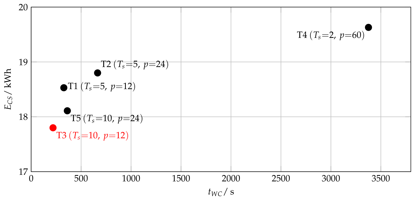
For the implementation of the NMPC, suitable values for the sampling time, prediction horizon, and control horizon must be selected to balance control performance and computational complexity. To this end, a parameter study was carried out in which different combinations of sampling time and prediction horizon were evaluated.

The study focused on two main performance indicators: (i) the auxiliary energy consumption of the cooling system, and (ii) the resulting computational effort of the NMPC optimization. The parameter study demonstrates that NMPC performance depends strongly on the selected sampling time and prediction horizon, with an appropriate balance between prediction capability and computational complexity being required to achieve good control performance. The investigated configurations and corresponding simulation results are summarized in

Table 6. Investigated NMPC parameter configurations for the MT cooling circuit and corresponding simulation results.

Test	${\mathit{T}}_{\mathit{s}}$ (s)	p	c	${\mathit{t}}_{\mathit{WC}}^{†}$ (s)	${\mathit{E}}_{\mathit{CS}}$ (kwh)
1	5	12	6	327	18.53
2	5	24	6	665	18.80
3	10	12	6	219	17.80
4	2	60	6	3376	19.63
5	10	24	6	362	18.11

^† Wall-clock execution time of the full MiL simulation; not to be confused with the simulated time horizon of the driving cycle.

and the relationship between computational effort and energy consumption is illustrated in Figure 11. As shown, configuration T3 ($T_s=10$ s, $p=12$, $c=6$) achieves the best performance on both indicators, with the lowest auxiliary energy consumption of $17.80$ $\mathrm{kWh}$ and the shortest simulation time of 219 $\mathrm{s}$. Although configuration T4 ($T_s=2 \mathrm{s}$, $p=60$) employs the finest temporal discretization and the largest prediction horizon in terms of prediction steps, it yields higher energy consumption than T3 despite sharing the same total look-ahead window of 120 s. Inspection of the NLP solver status confirmed successful convergence at each control step, ruling out solver failure as the cause. The degraded performance is therefore attributed to the substantially increased optimization problem size associated with the finer discretization, which increases computational complexity and may negatively affect numerical conditioning and optimization efficiency. Consequently, the additional prediction steps do not translate into improved closed-loop performance, indicating diminishing returns from further refinement of the prediction horizon. This result motivates the selection of a moderate sampling time and prediction horizon, as in T3, which achieves the best balance between solution quality and computational efficiency.

Here, $t_{WC}$ represents the simulation time and $E_{CS}$ the total consumed energy of the cooling system (fans + pump).

3.12. Sensitivity Analysis of NMPC Weighting Factors

To assess the robustness of the proposed NMPC strategy with respect to the selection of weighting factors $K_1$ and $K_2$, a sensitivity analysis was performed for the SeLv cycle at an ambient temperature of 40 °C. Seven weight combinations were evaluated, systematically varying $K_1$ and $K_2$ independently around the selected configuration ($K_1=50$, $K_2=0.02$). The results are summarized in

Table 7. Sensitivity analysis of NMPC weighting factors. SeLv cycle, $T_{\mathrm{amb}}=40 °\mathrm{C}$. The configuration marked with * violates the thermal constraint $T_{\mathrm{c}\mathrm{l}1,\max }\le 60 °\mathrm{C}$. The row in bold ($K_1=50$, $K_2=0.02$) corresponds to the configuration selected for all subsequent simulations in this work.

${\mathit{K}}_1$	${\mathit{K}}_2$	${\overline{\mathit{T}}}_{\mathbf{c}\mathbf{l}1}$ (°C)	${\mathit{T}}_{\mathbf{c}\mathbf{l}1,\mathbf{max}}$ (°C)	${\mathit{E}}_{\mathbf{CS}}$ (kWh)	${\mathit{e}}_{\mathbf{CS}}$ (kWh/km)
10	0.02	53.75	59.12	11.86	0.02156
50	0.02	52.42	58.98	17.80	0.03236
200	0.02	52.37	58.99	19.53	0.03551
50	0.005	52.36	58.99	19.29	0.03551
50	0.08	53.43	59.03	13.71	0.02394
10	0.08	56.14	61.80 *	5.12	0.00931
200	0.005	52.33	58.97	19.93	0.03635

.

The results demonstrate that the proposed NMPC strategy exhibits consistent qualitative behavior across a wide range of weighting factor combinations. Increasing $K_1$ while holding $K_2$ constant leads to tighter temperature regulation at the cost of higher auxiliary energy consumption, while increasing $K_2$ reduces energy demand with only minor variation in the average and maximum coolant temperature. This confirms that the two weighting factors influence the cost function in physically interpretable and independently separable ways.

The corner case $K_1=10$, $K_2=0.08$ demonstrates that an excessively low temperature penalty relative to the energy penalty results in violation of the 60 °C thermal constraint, with a maximum coolant temperature of $61.80$ °C. This defines a practical lower bound on $K_1$ for thermally safe operation and confirms that weight selection cannot be made arbitrarily without regard to thermal constraints.

Across all six thermally feasible configurations, the relative cooling system energy consumption ranges from 0.02156 kWh/km to 0.03635 kWh/km, remaining below the PI baseline of 0.03640 kWh/km in every case and below the rule-based baseline of 0.03532 kWh/km in the majority of configurations. This confirms that the energy-efficiency advantage of the proposed NMPC strategy over conventional control approaches is not an artifact of a specific weight configuration but holds robustly across the investigated tuning range. The selected configuration $K_1=50$, $K_2=0.02$ achieves a balanced trade-off between temperature regulation and energy efficiency and lies comfortably within the feasible operating region. Although lower cooling-system energy consumption can be achieved for certain weight combinations, the selected configuration was chosen based on its overall performance across all investigated driving cycles and ambient conditions. It provides a robust compromise between thermal safety margin, temperature regulation quality, and auxiliary energy demand, avoiding operation close to the thermal constraint boundary.

3.13. Selected NMPC Parameters

The NMPC parameters selected based on the parameter study discussed above are summarized in

Table 8. NMPC parameter configuration.

Parameter	Symbol	Value	Unit
Sampling time	$T_s$	10	$\mathrm{s}$
Prediction horizon	p	12	–
Control horizon	c	6	–
Weighting factor (temp.)	$K_1$	50	–
Weighting factor (energy)	$K_2$	0.02	–

.

3.14. Actuator Bounds and Rate Constraints

The actuator bounds enforce the physical operating limits of the cooling system. The pump speed is constrained to a minimum of 1400 rpm (20% of the maximum rated speed of 7000 rpm) to prevent thermal hotspots and ensure continuous coolant circulation, and to a maximum of 5600 rpm (80% of rated speed) due to the pressure limitations of the cooling circuit. The fan speed lower bound is set to approximately zero, allowing the controller to shut the fan off entirely when not required, with the upper bound corresponding to the rated fan speed of 2570 rpm. The rate constraints limit the change in actuator speed per control step, preventing excessive mechanical stress and ensuring smooth actuation. The complete actuator bounds and rate constraints are summarized in

Table 9. NMPC actuator bounds and rate constraints ($T_s=10 \mathrm{s}$).

Actuator	${\mathit{u}}_{min}$	${\mathit{u}}_{max}$	$\mathsf{\Delta }{\mathit{u}}_{min}$	$\mathsf{\Delta }{\mathit{u}}_{max}$
$n_{\mathrm{fan}}$ [rpm]	$\approx 0$	2570	$-514$ rpm/step	$+514$ rpm/step
$n_{\mathrm{pump}}$ [rpm]	1400	5600	$-1400$ rpm/step	$+1400$ rpm/step

.

3.15. Disturbance Prediction and State Availability

In the MiL evaluation presented in this work, the future trajectories of all disturbance variables (vehicle speed, motor heat generation, auxiliary heat load, oil mass flow, and ambient temperature) are supplied to the NMPC directly from the simulation environment over the full prediction horizon. This corresponds to a perfect-preview assumption, which is standard practice in MiL-based NMPC evaluation and allows the controller’s theoretical energy-saving potential to be assessed independently of prediction uncertainty. In a real vehicle deployment, future disturbance trajectories would need to be estimated from available information sources such as route data, historical driving profiles, or short-horizon prediction models, which would introduce prediction errors not considered in the present study.

The sensitivity of the proposed controller to prediction errors is partially mitigated by the receding-horizon implementation: at each sampling instant, the realized disturbance values are fed back as initial conditions for the subsequent prediction, limiting the propagation of prediction errors between control steps. Given the dominant thermal time constant of the system (approximately 192 $\mathrm{s}$, discussed in Section 3.4) and the 10 $\mathrm{s}$ sampling interval, thermal states evolve slowly relative to the correction frequency, providing a degree of inherent robustness to short-term prediction inaccuracies. A quantitative sensitivity analysis with realistic prediction models is identified as a direction for future work.

In the MiL environment, all five model states are available directly from the simulation at each sampling instant. In a real vehicle, the states $T_M$ and $T_{\mathrm{oil}}$ are not directly measurable with standard sensor configurations and would require a state estimator for practical deployment. State estimation for fuel-cell truck thermal management systems has been investigated separately within the broader research context of this work and is identified as a prerequisite for hardware-in-the-loop and vehicle-level implementation, alongside the real-time code feasibility discussed in Section 4.6.

A sensitivity analysis of the controller performance to velocity prediction uncertainty was conducted within the research group as part of the broader investigation of this thermal management system. The results indicate that, when the receding-horizon disturbance correction is active, prediction errors of the order of $\pm 30\%$ in vehicle speed have negligible influence on thermal constraint satisfaction and minor influence on energy consumption. This is consistent with the physical argument above: the dominant thermal time constant of approximately 192 $\mathrm{s}$ strongly attenuates short-term prediction errors before they can significantly affect the bulk component temperatures used for cooling actuation. A full quantitative sensitivity study with realistic prediction models, including route-based forecasting and stochastic uncertainty, is nevertheless identified as a direction for future work.

4. Results

The following section presents the simulation results of the proposed NMPC strategy in comparison with the rule-based and PI benchmark controllers. After introducing the design and parameterization of both benchmark controllers, the performance is evaluated across three driving cycles and three ambient temperature conditions. The per-cycle results are subsequently synthesized to draw conclusions regarding the energy-saving potential and thermal management performance of the proposed strategy, followed by an assessment of its real-time feasibility.

4.1. Benchmark Controller Design

For benchmarking purposes, the proposed NMPC strategy is compared in MiL with two conventional control strategies: a rule-based (RB) controller and a PI controller. The RB controller corresponds to the baseline strategy implemented in the investigated vehicle during the project development phase, designed to ensure robust thermal protection and stable operation under all considered operating conditions rather than to minimize auxiliary energy consumption; consequently, no systematic parameter optimization or retuning of its thresholds was performed within this study. To provide a more balanced benchmark against a conventionally tuned feedback controller, an additional PI-based strategy was implemented and tuned for coolant temperature regulation.

The RB controller regulates the coolant pump and radiator fan independently via predefined lookup table-based threshold logic, without an explicit setpoint comparison. The pump speed, as a percentage of its maximum, is a piecewise-linear function of the coolant temperature $T_{cl1}$: constant at its minimum value below 30 °C, increasing linearly to its maximum value by 50 °C, and saturating above this temperature. The fan duty cycle follows a similarly piecewise-linear function once active, floored at a minimum of 20% and gated by a hysteresis switch with an on-threshold of 45 °C and an off-threshold of 40 °C: the fan remains off until the coolant temperature reaches 45 °C, at which point it engages and follows the ramp shown in

Table 10. Rule-based controller lookup table definitions and actuator ranges.

Actuator	${\mathit{T}}_{\mathit{c}\mathit{l}1}$ Breakpoints [°C]	Output [%]
Pump	$-20,30,50,70,80$	$20,20,80,80,80$
Fan (while active) 1	$20,40,50,80$	$0,20,100,100$

¹ Fan output floored at 20% while active; hysteresis on/off thresholds at 45 °C/40 °C. Pump output range corresponds to 1400–5600 rpm (20–80% of 7000 rpm); fan output range corresponds to 0–2570 rpm (0–100%).

, reaching 100% duty cycle by 50 °C and remaining engaged until the temperature falls back below 40 °C. The exact breakpoints and corresponding actuator outputs are summarized in Table 10.

The PI controller comprises two independent PI loops (no derivative action, i.e., $D=0$ in both), each regulating $T_{cl1}$ toward a common setpoint of 48 °C and driving one actuator directly. No explicit output-distribution or split-range logic is used between the two loops; instead, owing to their independent tuning, the pump loop reaches its actuator saturation limit at a smaller temperature error than the fan loop, so that the pump acts as the primary actuator for small corrections while the fan engages more strongly only once a larger corrective action is required. This sequencing is therefore a consequence of the relative tuning of the two loops rather than an explicit coordination scheme. Both loops were tuned independently using the frequency-response-based automated tuning method in Simulink Control Design, with clamping anti-windup. The resulting gains, sample time, and actuator limits are summarized in

Table 11. PI controller parameters for the fan and pump loops.

Parameter	Fan Controller	Pump Controller
Controller type	PI	PI
Sample time, $T_s$	1 s	1 s
Setpoint	48 °C	48 °C
Proportional gain, P	10,000	43,563.933
Integral gain, I	500	9759.3904
Derivative gain, D	0	0
Anti-windup method	Clamping	Clamping
Output/integrator limits	0.01–100%	1400–5600 rpm
Output scaling	$\times 2570/100\to n_{fan}$	$\times 7000/100\to n_{pump}$
Tuning method	Frequency-response-based	Frequency-response-based

. The pump’s actuator range (20–80% of 7000 rpm) and the fan/pump output scaling are identical between the RB and PI controllers, ensuring a consistent basis for comparison between the two benchmark strategies.

4.2. SeLv Cycle

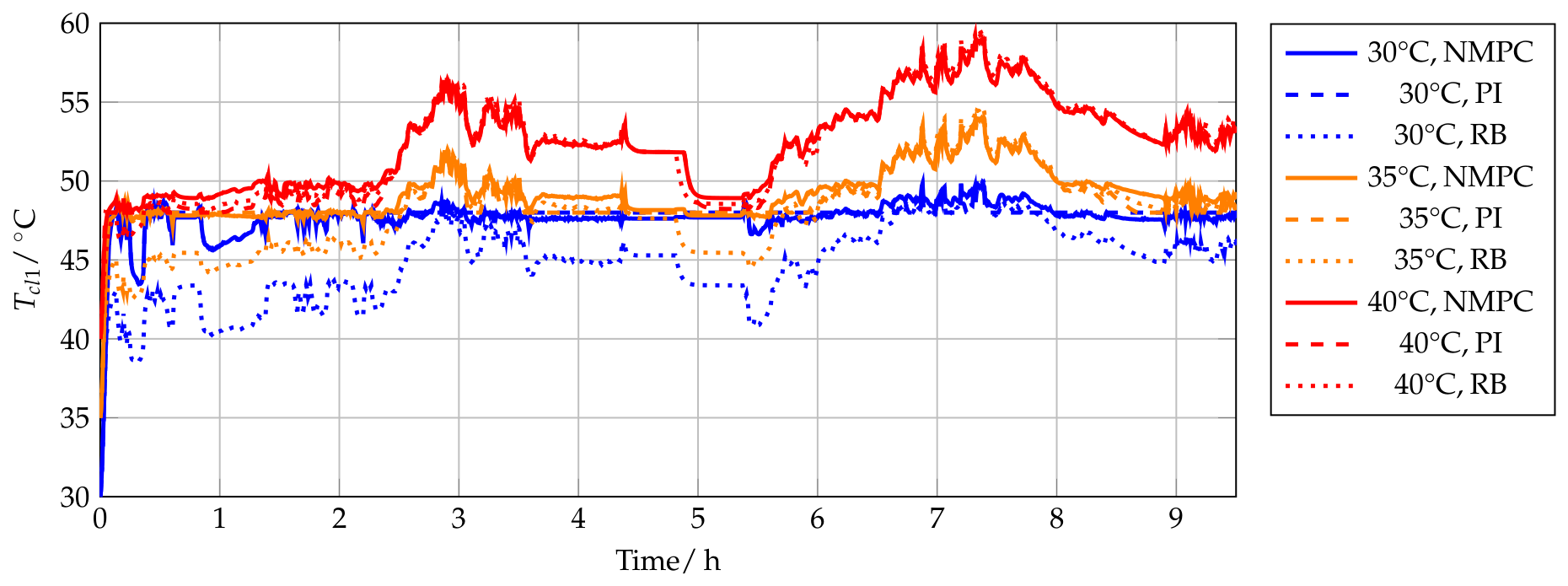
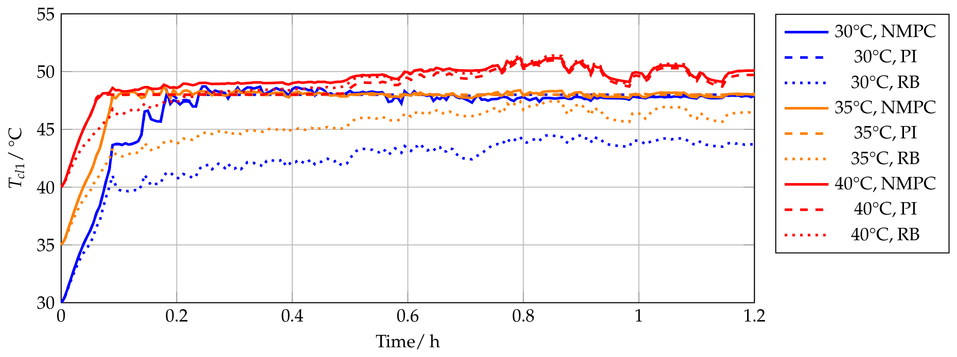
The simulation results for the SeLv driving cycle are presented and discussed for the different control strategies and ambient temperatures. Figure 12 shows the coolant temperature $T_{cl1}$ for all controllers. For all cases, the target coolant temperature is set to 48 °C, as defined in Section 3.11.

From Figure 12, it is evident that the RB control strategy implemented in the vehicle significantly overshoots the required cooling demand, resulting in coolant temperatures that are lower than necessary. This behavior leads to excessive auxiliary energy consumption without providing any operational benefit, as fuel-cell derating only occurs at temperatures above 48 °C. This effect is particularly pronounced at ambient temperatures of 30 °C and 35 °C.

The ambient temperature of 40 °C represents an extreme operating condition, under which all controllers exceed the target coolant temperature, as the cooling system is designed to tolerate coolant temperatures up to 60 °C. Nevertheless, a clear tendency can be observed for the NMPC strategy to allow slightly higher coolant temperatures in order to reduce auxiliary energy consumption.

The quantitative comparison of the control strategies for the SeLv cycle is summarized in

Table 12. Comparison of NMPC, PI, and RB controllers at different ambient temperatures (SeLv cycle). Energy reduction indicates the relative reduction in cooling system energy consumption achieved by NMPC compared to the respective baseline controller.

${\mathit{T}}_{\mathit{amb}}$ (°C)	Controller	${\mathit{e}}_{\mathit{CS}}$ (kWh/km)	${\mathit{e}}_{\mathit{CS}}$ red. (%)	${\overline{\mathit{T}}}_{\mathit{c}\mathit{l}1}$ (°C)	${\mathit{T}}_{\mathit{c}\mathit{l}1,max}$ (°C)
30	NMPC	0.00931	–	47.68	49.85
	PI	0.01083	14.02	47.78	49.48
	RB	0.01685	44.75	44.88	50.00
35	NMPC	0.02174	–	49.15	54.04
	PI	0.02519	13.69	48.85	54.01
	RB	0.02736	20.56	48.13	54.48
40	NMPC	0.03234	–	52.42	58.97
	PI	0.03640	11.14	52.16	58.98
	RB	0.03532	8.43	52.34	59.44

. For all investigated ambient temperatures, the NMPC consistently achieves the lowest cooling system energy consumption. Depending on the ambient condition, energy savings of up to 45% compared to the rule-based controller and up to 14% compared to the PI controller are obtained.

Notably, these energy savings are achieved without a significant increase in either the average or the maximum coolant temperature. Across all ambient temperatures, the average coolant temperature under NMPC operation differs by less than $1 °\mathrm{C}$ from the PI and rule-based controllers, while the maximum coolant temperatures remain nearly identical. This indicates that the reduction in cooling energy consumption is not achieved at the expense of increased thermal peak loads or reduced thermal safety margins.

This behavior can be attributed to the optimization-based nature of the NMPC strategy. Rather than strictly enforcing a fixed coolant temperature setpoint, the NMPC allows small, controlled deviations in coolant temperature to reduce fan and pump operation, as explicitly reflected in the cost function. As a result, a more energy-efficient operation of the medium-temperature cooling circuit is achieved, particularly under the predominantly steady-state operating conditions of the SeLv driving cycle.

Table 13. Component temperatures for the SeLv cycle: mean and maximum values for NMPC, PI, and RB controllers across all investigated ambient temperature conditions. Thermal limits are indicated in the final row.

Controller	${\mathit{T}}_{\mathbf{amb}}$ [°C]	${\mathit{T}}_{\mathbf{aux}}$ [°C]		${\mathit{T}}_{\mathbf{c}\mathbf{l}2}$ [°C]		${\mathit{T}}_{\mathit{M}}$ [°C]		${\mathit{T}}_{\mathbf{oil}}$ [°C]
		Mean	Max	Mean	Max	Mean	Max	Mean	Max
NMPC	30	61.8	65.8	44.3	47.6	52.7	67.7	51.9	64.6
	35	63.3	70.0	47.0	52.0	54.5	70.4	53.5	67.4
	40	66.6	75.0	50.9	56.9	58.2	75.2	57.1	72.2
PI	30	61.8	65.4	44.5	47.3	52.6	66.7	51.7	63.6
	35	62.9	70.0	46.8	51.9	54.0	70.3	53.0	67.3
	40	66.3	75.0	50.7	56.9	58.0	75.2	56.9	72.2
RB	30	58.9	66.0	43.1	47.8	50.7	67.8	49.7	64.7
	35	62.2	70.5	46.5	52.4	54.3	71.6	53.2	68.5
	40	66.4	75.5	50.8	57.3	58.7	76.5	57.5	73.3
Limit	–	<85		<60		<110		<90

reports the component temperatures for the SeLv cycle, which represents the most thermally demanding conditions investigated in this work; all thermal limits are satisfied across all controllers and ambient temperatures, with the highest component temperatures occurring at 40 °C ambient.

4.3. VECTO Long Haul

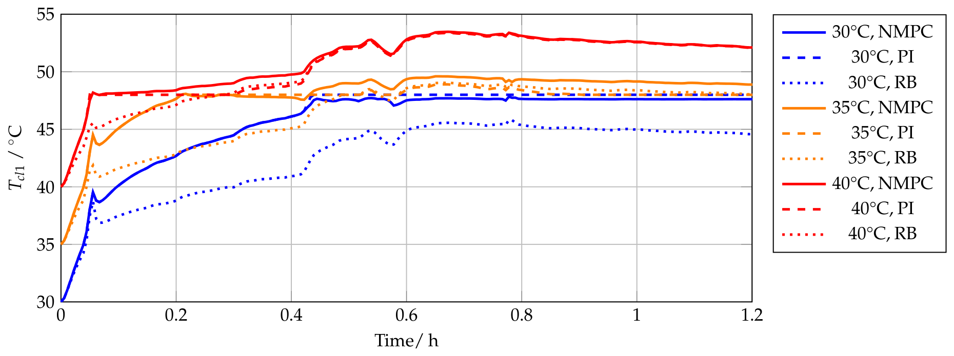
Similar to the SeLv cycle, ambient temperature strongly influences the medium-temperature cooling circuit, shifting the operating temperature level for all control strategies (Figure 13). For the VECTO Long Haul cycle, all controllers achieve stable temperature regulation without oscillatory behavior. The RB strategy consistently overcools the system due to conservative safety margins, while the PI controller regulates close to the target setpoint of 48 °C at lower ambient temperatures, but cannot reach it at 40 °C due to system limitations. In contrast, the NMPC allows small temperature deviations to minimize fan and pump operation, resulting in energy-efficient operation within acceptable thermal limits.

Table 14. Comparison of NMPC, PI, and RB controllers at different ambient temperatures (VECTO Long Haul cycle). Energy reduction indicates the relative reduction in cooling system energy consumption achieved by NMPC compared to the respective baseline controller.

${\mathit{T}}_{\mathit{amb}}$ (°C)	Controller	${\mathit{e}}_{\mathit{CS}}$ (kWh/km)	${\mathit{e}}_{\mathit{CS}}$ red. (%)	${\overline{\mathit{T}}}_{\mathit{c}\mathit{l}1}$ (°C)	${\mathit{T}}_{\mathit{c}\mathit{l}1,max}$ (°C)
30	NMPC	0.00293	–	45.76	47.83
	PI	0.00302	3.15	46.03	48.01
	RB	0.00845	66.90	42.76	45.83
35	NMPC	0.01209	–	48.04	49.60
	PI	0.01727	30.03	47.47	48.91
	RB	0.01726	29.98	46.44	49.04
40	NMPC	0.02132	–	51.08	53.47
	PI	0.02390	10.82	50.86	53.38
	RB	0.02455	13.15	50.65	53.43

summarizes the energy performance. The NMPC achieves the lowest cooling system energy consumption across all ambient conditions, with savings of up to 67% compared to RB and up to 30% compared to PI. These savings are achieved without significant increases in average or maximum coolant temperature, which remain comparable to PI and within safe operating limits. Overall, the NMPC avoids unnecessary cooling during extended steady-state operation, reducing energy use while maintaining thermal safety.

The component temperatures for the VECTO Long Haul cycle are reported in

Table 15. Component temperatures for the VECTO Long Haul cycle: mean and maximum values for NMPC, PI, and RB controllers across all investigated ambient temperature conditions. Thermal limits are indicated in the final row.

Controller	${\mathit{T}}_{\mathbf{amb}}$ [°C]	${\mathit{T}}_{\mathbf{aux}}$ [°C]		${\mathit{T}}_{\mathbf{c}\mathbf{l}2}$ [°C]		${\mathit{T}}_{\mathit{M}}$ [°C]		${\mathit{T}}_{\mathbf{oil}}$ [°C]
		Mean	Max	Mean	Max	Mean	Max	Mean	Max
NMPC	30	59.5	63.8	42.0	45.3	48.2	56.0	47.9	55.1
	35	61.8	65.5	45.7	47.7	51.0	58.4	50.4	56.8
	40	64.9	69.4	49.5	52.0	54.8	61.6	54.1	60.3
PI	30	59.7	64.2	42.1	45.8	48.5	56.3	48.2	55.6
	35	61.3	64.8	45.2	47.2	50.6	58.0	49.9	56.2
	40	64.7	69.3	49.3	51.9	54.6	61.3	53.9	60.1
RB	30	56.5	61.5	41.0	44.2	46.1	53.2	45.5	52.2
	35	60.2	65.0	45.0	47.4	50.2	57.2	49.5	55.9
	40	64.5	69.3	49.3	52.0	54.7	61.4	53.9	60.2
Limit	–	<85		<60		<110		<90

, confirming that the thermal limits of the motor winding, motor oil, and auxiliary components are respected by all three controllers across all investigated ambient conditions.

4.4. VECTO Urban Delivery

Figure 14 shows the coolant temperature ($T_{cl1}$) for the different controllers during the VECTO Urban Delivery cycle. Unlike long-haul operation, the urban delivery profile is characterized by frequent load changes and pronounced transients, placing higher demands on the thermal management system.

The results for this cycle are summarized in

Table 16. Comparison of NMPC, PI, and rule-based RB controllers at different ambient temperatures (VECTO Urban Delivery cycle). Energy reduction indicates the relative reduction in cooling system energy consumption achieved by NMPC compared to the respective baseline controller.

${\mathit{T}}_{\mathit{amb}}$ (°C)	Controller	${\mathit{e}}_{\mathit{CS}}$ (kWh/km)	${\mathit{e}}_{\mathit{CS}}$ red. (%)	${\overline{\mathit{T}}}_{\mathit{c}\mathit{l}1}$ (°C)	${\mathit{T}}_{\mathit{c}\mathit{l}1,max}$ (°C)
30	NMPC	0.00194	–	46.78	48.72
	PI	0.00196	1.14	46.84	48.01
	RB	0.00724	73.25	42.30	44.52
35	NMPC	0.00515	–	47.50	48.78
	PI	0.00852	39.57	47.46	48.10
	RB	0.01233	58.25	45.23	47.45
40	NMPC	0.01702	–	49.32	51.18
	PI	0.02289	25.63	48.81	50.97
	RB	0.02259	24.65	48.91	51.39

. Across all ambient temperatures, the NMPC achieves the lowest cooling system energy consumption. Compared to the rule-based controller, energy savings reach up to 73% at 30 °C, while savings of up to 40% are obtained relative to the PI controller at 35 °C. Even at 40 °C, where the system operates near its thermal limits, the NMPC maintains energy savings of approximately 25%.

Despite these reductions in cooling energy, average and maximum coolant temperatures remain comparable to the PI controller and indicate no additional thermal stress. The rule-based controller exhibits lower average temperatures due to conservative overcooling, whereas the NMPC effectively limits temperature peaks while reducing fan and pump operation, demonstrating energy-efficient transient thermal management.

Component temperatures for the VECTO Urban Delivery cycle are summarized in

Table 17. Component temperatures for the VECTO Urban Delivery cycle: mean and maximum values for NMPC, PI, and RB controllers across all investigated ambient temperature conditions. Thermal limits are indicated in the final row.

Controller	${\mathit{T}}_{\mathbf{amb}}$ [°C]	${\mathit{T}}_{\mathbf{aux}}$ [°C]		${\mathit{T}}_{\mathbf{c}\mathbf{l}2}$ [°C]		${\mathit{T}}_{\mathit{M}}$ [°C]		${\mathit{T}}_{\mathbf{oil}}$ [°C]
		Mean	Max	Mean	Max	Mean	Max	Mean	Max
NMPC	30	57.3	59.6	43.4	46.6	44.5	52.3	44.7	52.3
	35	58.1	59.8	45.4	47.0	47.7	54.8	47.6	54.7
	40	60.0	62.3	48.1	49.9	51.0	57.5	50.8	57.4
PI	30	57.4	59.8	43.3	46.4	44.5	52.3	44.8	52.3
	35	58.1	59.8	46.1	47.4	47.6	54.9	47.6	54.8
	40	59.5	62.1	47.8	49.7	50.7	57.0	50.4	56.9
RB	30	52.9	55.6	41.0	43.1	43.5	50.7	43.4	50.6
	35	55.9	58.6	44.1	46.0	47.4	54.3	47.1	54.2
	40	59.6	62.5	47.9	50.1	51.5	58.2	51.2	58.1
Limit	–	<85		<60		<110		<90

; consistent with the other investigated cycles, all thermal limits are respected and the temperature profiles of NMPC and PI remain comparable across all ambient conditions.

These results highlight that the primary benefit of NMPC in urban driving scenarios lies in its predictive capability, allowing the medium-temperature cooling circuit to operate closer to its optimal thermal range. This leads to a significant reduction in auxiliary energy consumption without compromising thermal safety.

4.5. Synthesis Across Driving Cycles

The analysis of the SeLv, VECTO Long Haul, and VECTO Urban Delivery cycles shows that the benefits of model predictive control depend strongly on driving dynamics. All cycles show reduced energy consumption of the cooling system with NMPC, but the extent and mechanisms differ.

For the VECTO Long Haul cycle, dominated by steady-state operation, NMPC mainly prevents conservative overcooling, yielding moderate energy savings without affecting average or maximum coolant temperatures. In the SeLv cycle, with mixed steady and transient operation, NMPC balances temperature regulation and cooling energy more effectively, reducing auxiliary demand while maintaining safe temperatures. The greatest relative savings occur in the VECTO Urban Delivery cycle, where frequent stop-and-go and load transients cause reactive controllers to overreact. Here, NMPC anticipates thermal loads, significantly lowering energy consumption and limiting temperature peaks.

It should be noted that the rule-based controller represents the strategy implemented in the vehicle during the project development phase and was designed primarily for thermal robustness rather than energy efficiency. No systematic tuning or optimization of its control thresholds was performed within this study. The large energy savings observed relative to the RB strategy therefore partly reflect this design intent rather than an inherent limitation of rule-based control in general. The PI controller, tuned for coolant temperature regulation, serves as a more conservative benchmark and confirms that the NMPC achieves meaningful efficiency gains also against a conventionally optimized feedback strategy.

Across all cycles, energy savings from NMPC do not come at the cost of higher average or maximum temperatures. Instead, NMPC keeps the cooling system closer to its optimal thermal range by balancing temperature control and energy use, demonstrating that its primary advantage lies in adaptive, intelligent thermal management rather than aggressive cooling.

Averaged across all investigated driving cycles and ambient temperatures, the mean steady-state deviation from the 48 °C reference is approximately $1.6$ $°\mathrm{C}$ for NMPC, $1.5$ $°\mathrm{C}$ for PI, and $2.9$ $°\mathrm{C}$ for RB, consistent with the RB controller’s conservative, non-setpoint-tracking design intent.

4.6. Real-Time Feasibility of the NMPC Implementation

To assess the real-time applicability of the proposed NMPC controller, both solver execution characteristics and Simulink profiling results are analyzed. All simulations were performed on a desktop workstation equipped with an 11th Gen Intel Core i7-11800H processor ($2.30$ $\mathrm{G}$$\mathrm{Hz}$) and 32 $\mathrm{GB}$ of RAM, running Windows 11 Enterprise (64-bit) and MATLAB/Simulink R2026a. The evaluation considers the solver time distribution as well as the simulation step size to ensure consistency between numerical resolution and controller execution requirements.

The Simulink model operates with a variable-step solver; automatic solver selection resolved to ode15s, a stiff-system solver suited to models with widely separated time constants such as the thermal dynamics investigated in this work. The relative tolerance was set to $1\times {10}^{-3}$, with an initial absolute tolerance of $1\times {10}^{-6}$ and automatic absolute tolerance scaling enabled; the maximum step size was limited to 1 $\mathrm{s}$.

Under these settings, the simulation used an average solver step size of approximately $0.39$ $\mathrm{s}$, with the maximum step size reached in only $0.54\%$ of steps, indicating stable numerical integration behavior and no excessive refinement of the dynamic simulation. The simulation is therefore sufficiently coarsened relative to the controller sampling time, avoiding unnecessary computational overhead. The complete simulation (34,895 s of simulated time) required $261.14$ $\mathrm{s}$ of wall-clock run time, corresponding to a run-time-to-simulation-time ratio of $7.48\times {10}^{-3}$, i.e., the full model-in-the-loop simulation, including both plant dynamics and controller, executed approximately 134 times faster than real time.

In addition to the overall solver performance, the computational burden of the NMPC block specifically was evaluated using the Simulink Profiler. Over the full simulation horizon, the NMPC block was executed 3495 times, with a total execution time of $160.865\mathrm{s}$. This results in an average computation time per control step of

$$t_{\mathrm{NMPC}}={\displaystyle \frac{160.865}{3495}}=0.046 \mathrm{s}$$

(37)

For a sampling time of $T_s=10 \mathrm{s}$, the real-time feasibility factor is defined as

$$\mathrm{RTF}={\displaystyle \frac{t_{\mathrm{NMPC}}}{T_s}}$$

(38)

resulting in $\mathrm{RTF}=0.0046$, which is well below unity. This result was consistent in magnitude across simulations at different ambient temperatures, indicating stable computational behavior across operating conditions. The remaining simulation time is primarily attributed to model dynamics and non-NMPC components, confirming that the controller itself is not the computational bottleneck of the system.

It should be noted that this evaluation reflects average execution time on a desktop development platform within MATLAB/Simulink rather than a maximum or high-percentile execution time, and that the controller was not tested as generated code on representative embedded automotive hardware. Embedded implementation would require code generation via Simulink Coder or Embedded Coder and subsequent validation on the target electronic control unit (ECU), which typically differs substantially from a development workstation in CPU architecture, available clock speed, and memory constraints. The reported real-time feasibility should therefore be regarded as a preliminary indication based on average-case desktop simulation performance, rather than a confirmed result for embedded deployment; dedicated hardware-in-the-loop testing on representative automotive hardware is identified as a direction for future work.

5. Discussion

The discussion is structured into four parts: an interpretation of the results, a comparison with existing studies, a revisiting of the research objectives, and a summary of limitations.

5.1. Interpretation of Results

The results demonstrate that the effectiveness of predictive thermal management strongly depends on the dynamic characteristics of the driving cycle. Under predominantly steady-state operating conditions, such as the VECTO Long Haul cycle, all investigated controllers operate close to a thermal equilibrium, limiting the achievable energy savings. In this case, the NMPC mainly reduces conservative overcooling compared to the rule-based strategy.

In contrast, the benefits of NMPC become more pronounced for highly dynamic driving profiles with frequent load changes and transient cooling demands. Particularly for the SeLv and VECTO Urban Delivery cycles, the predictive controller is able to anticipate future thermal loads and adjust actuator operation proactively. This reduces unnecessary fan and pump actuation compared to reactive control approaches and leads to significantly lower auxiliary energy consumption.

At the same time, the reduced cooling energy demand is not accompanied by a noticeable increase in average or maximum coolant temperature. The comparable temperature levels observed for the NMPC and PI controller indicate that the achieved savings primarily result from a more efficient utilization of the available cooling capacity rather than from relaxed thermal constraints. This suggests that predictive thermal management can improve auxiliary efficiency without compromising thermal protection requirements for fuel-cell heavy-duty applications.

5.2. Comparison with Existing Studies

Table 18. Comparison of NMPC-based thermal management studies.

Reference	Vehicle	System	Benchmark	Savings	Thermal Model Validation ‡
Batool et al. [19]	FCEV HD	Energy + TMS	RB	2.28% †	Experiment
Varlese et al. [20]	FC electric tractor	TMS	PI	30%	Experiment
Schutzeich et al. [16]	BEV *	TMS	RB	37.9%	Experiment mentioned, not presented
Hajidavalloo et al. [17]	BEV *	Battery + cabin	RB	+1–2 h range	Simulation
Ma et al. [18]	BEV *	Battery heating	PID	18.18%	Simulation
Xu et al. [21]	BEV *	Powertrain + cooling	RB	1.06%	Simulation
This work	FCEV HD	MT cooling circuit	RB + PI	16.6% (avg.) 39.6% (max) vs. PI	Experiment

BEV: battery electric vehicle; FC: fuel cell; FCEV: fuel-cell electric vehicle; HD: heavy duty; MT: medium-temperature; TMS: thermal management system; ^† savings on vehicle level; * passenger vehicle; ^‡ closed-loop controller evaluation was performed in simulation or model-in-the-loop environments in all listed studies unless otherwise stated.

contextualizes the energy savings achieved in this work relative to representative NMPC-based thermal management studies from the literature. While direct numerical comparison is limited by differences in vehicle type, controlled subsystem, and benchmark strategy, several observations can be made.

The results of this work are consistent with results reported in studies on comparable systems. Notably, the NMPC savings relative to the PI controller (up to 39.6%) are in line with comparable literature studies. To the authors’ knowledge, this work is among the few that validate the prediction model against physical test bench measurements rather than relying solely on simulation-based validation. While this does not substitute for closed-loop controller validation, it reduces a key source of uncertainty in the MiL results by grounding the prediction model in real-system behavior.

5.3. Revisiting the Research Objectives

The first objective of this work was to establish a structured and experimentally grounded methodology for predictive thermal management of heavy-duty fuel-cell vehicle cooling systems. This objective was achieved through the development of an end-to-end workflow covering control-oriented modeling, systematic parameter estimation from drivetrain test bench measurements, and NMPC design and evaluation for the medium-temperature cooling circuit of a fuel-cell heavy-duty truck.

The second objective was to investigate whether lumped-parameter thermal models identified from experimental data provide sufficient accuracy for predictive control applications while remaining computationally tractable for real-time optimization. The obtained validation results, with coefficients of determination above 0.9 and normalized root mean square errors below 10%, demonstrate that the developed prediction model accurately reproduces the thermal dynamics of the investigated cooling system. At the same time, the achieved solver times confirm the suitability of the proposed approach for NMPC implementation.

The third objective was to quantify the energy-saving potential of NMPC-based thermal management under representative heavy-duty operating conditions. The results showed that the predictive controller reduced cooling system energy consumption across all investigated driving cycles and ambient conditions, with the largest benefits observed for highly dynamic operating profiles. Compared to the tuned PI controller, energy savings of up to 39.6% (VECTO Urban Delivery cycle, 35 °C ambient) and an average of 16.6% across all investigated conditions were achieved without significant increases in average or maximum coolant temperatures and the steady-state deviation from the reference temperature remained comparable to that of the PI controller ($1.6$ $°\mathrm{C}$ vs. $1.5$ $°\mathrm{C}$, Section 4.5), indicating that the improved efficiency was obtained without compromising thermal protection requirements.

5.4. Limitations

The presented study is subject to several limitations. First, the controller evaluation was conducted in a model-in-the-loop environment assuming accurate availability of disturbance information, including vehicle speed and component heat losses. While this enables a controlled assessment of the predictive control strategy, real-vehicle operation is affected by measurement uncertainty and prediction errors, which were not considered within the scope of this work.

Second, the developed cooling system model is based on a lumped-parameter representation with effective heat-transfer coefficients identified from experimental data. While this approach is computationally efficient and sufficiently accurate for control-oriented applications, it cannot capture detailed spatial temperature distributions or explicit flow-dependent heat-transfer phenomena within individual components.

Furthermore, the investigation focused on the medium-temperature cooling circuit and did not consider interactions with additional thermal subsystems such as cabin conditioning or battery thermal management. The reported results are therefore limited to the investigated subsystem and operating conditions.

Finally, the controller assessment was limited to simulation-based evaluation using representative driving cycles. Experimental validation of the predictive controller in hardware-in-the-loop or vehicle-level operation remains part of future work.

6. Conclusions

This study investigated nonlinear model predictive control for the medium-temperature cooling circuit of a heavy-duty fuel-cell truck. The results show that predictive thermal management can reduce auxiliary cooling energy consumption compared to conventional rule-based and PI strategies, particularly under dynamic driving conditions, while maintaining comparable coolant temperature levels. The findings confirm the potential of predictive control to improve thermal management efficiency without compromising thermal safety in fuel-cell vehicle applications. Beyond the demonstrated energy savings, precise thermal management is increasingly recognized as important for component durability, since operating temperature has been shown to significantly influence degradation rates and state-of-health evolution in PEMFC systems [33]; while the present work focuses on the medium-temperature circuit, the proposed methodology may be similarly applicable to other thermally critical circuits, such as the fuel-cell high-temperature loop, where precise temperature control is directly linked to component lifetime. Future work will address robustness to measurement and prediction uncertainties, extend the validation toward hardware-in-the-loop and vehicle-level testing, and explore integration with broader energy-system concepts, including onboard or stationary thermal energy storage, to further improve overall system efficiency and flexibility.