Fault Location Method for Continuous Transmission Lines of High-Speed Railway Based on Low-Voltage Measurements at Box-Type Substations

Abstract

Precise fault localization for high-speed railway continuous transmission lines is indispensable for sustaining power supply reliability and mitigating power outages. This study presents a novel fault localization approach that uses low-voltage information obtained from box-type substations distributed along continuous transmission lines. The proposed scheme relies on the distribution features of the positive-to-negative sequence voltage ratio ($r_{PNV}$) measured at the low-voltage terminals of box-type substations. Results reveal that the magnitude of $r_{PNV}$ gradually declines from the main substation to the fault location in the fault upstream area, while it stays nearly unchanged in the downstream section. Based on this feature, the faulted section is initially determined by means of the nearest neighbor clustering method. Subsequently, the precise fault location is calculated by solving equations that combine the sequence voltage ratio at the fault point with the measurements obtained from the main substation and box-type substations downstream of the fault. The proposed method requires only asynchronous low-voltage measurements, eliminates the need for fault impedance modeling, and is applicable to various asymmetric faults. Simulation tests under different fault types, fault resistances (up to 2000 Ω), noise conditions, and neutral grounding modes demonstrate that the method achieves high accuracy and robustness.

1. Introduction

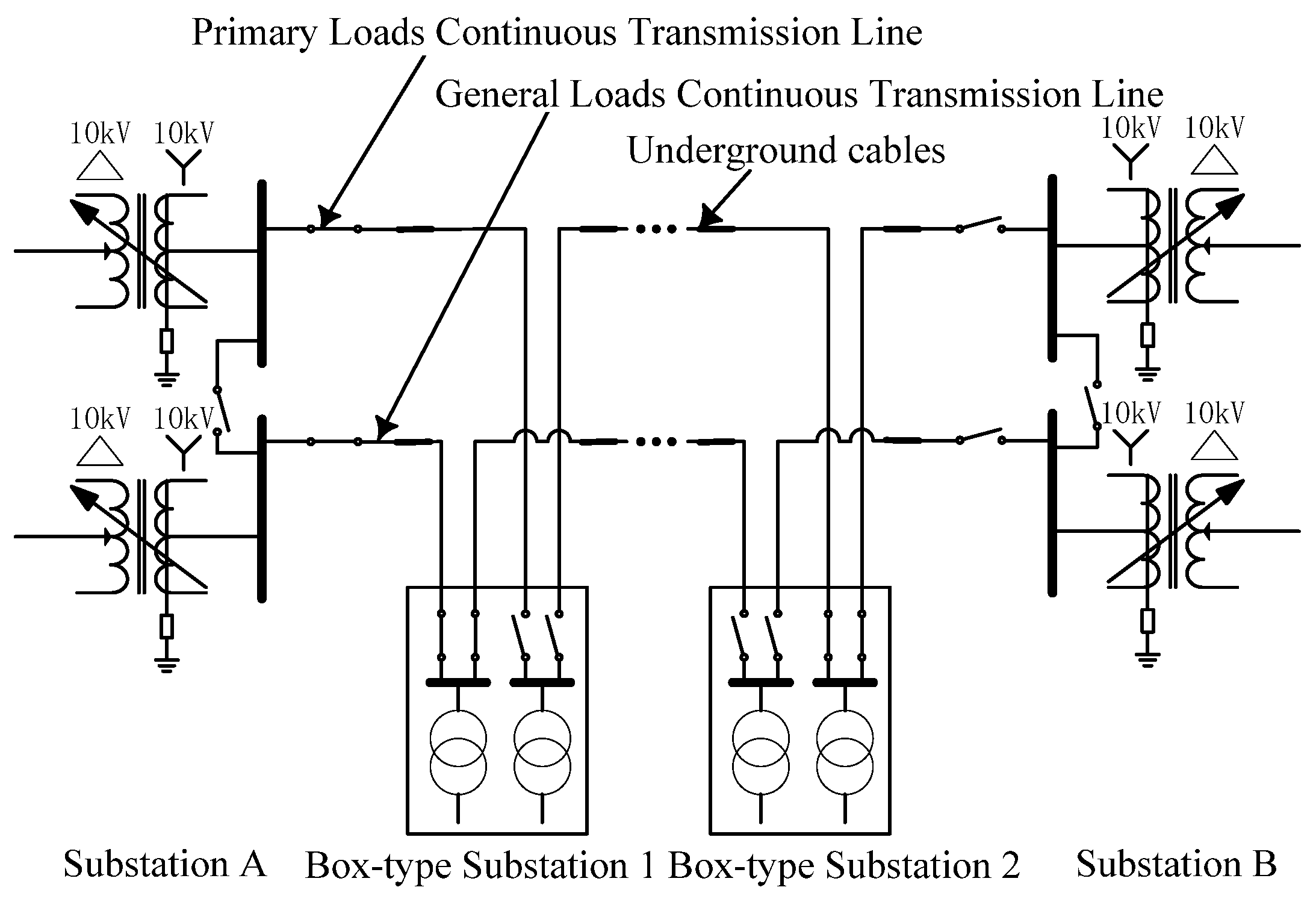
The 10 kV distribution network for the high-speed railway system plays a vital role in supporting the railway signaling, communication and other integrated electrical equipment. In China, underground cables are used for all lines within high-speed railway distribution systems. To prevent the generation of substantial capacitive current, these systems operate with low-resistance grounding, as visualized in Figure 1. Two 10 kV radial transmission lines are configured in the system, as shown in Figure 1 [1]. They are classified into two categories: continuous transmission lines for primary loads and those for general loads. These two 10 kV continuous transmission lines serve as mutual backup. The continuous transmission lines extend over a long distance and operate under harsh working conditions. Accordingly, it is essential to achieve accurate fault location for high-speed railway continuous transmission lines, so as to resume power supply quickly and greatly cut down outage time.

Three typical types of fault location schemes are widely adopted, namely impedance analysis [2,3,4,5,6,7], traveling wave–based [8] and intelligent [9,10] methods. Based on Kirchhoff’s laws, impedance analysis methods establish relevant equations with acquired voltage and current signals to solve for fault location distance. By solving the equations, the fault distance can be obtained. In [2], a method of fault location based on a new impedance matrix manipulation procedure has been proposed, in which load parameters are not required. Reference [3] presents a new fault location method using phase-domain equations of distributed line parameters. It works well for distributed generation and greatly improves fault location accuracy. In [4], an iterative modification method of capacitive current is proposed, which can decrease the uncertainty of complex equations caused by grounded capacitive current. For short-circuit fault detection and classification, a state estimation algorithm was developed in [5] and proven to deliver reliable and accurate results. Reference [6] presents a locating technique for low-current grounding faults based on the distribution characteristics of zero-sequence voltage. Due to the utilization of zero-sequence voltage, the results can avoid being affected by distributed generation. Reference [7] adopts the harmonic voltage ratio and sparse sensing technology, and it only requires low-cost voltage measurements. However, this method has not been verified in real-time experiments. In [8,9], fault distance is optimized by incorporating both normal operation data and fault data based on μPMU phasor information. When a fault occurs, high-frequency traveling waves are excited in the transmission lines. Traveling wave methods adopt the arrival time of these waves at measuring points to estimate the fault distance. In [10], the active location method adopting cascaded H-bridge structures can work stably regardless of fault inception angles, while lowering the standards for signal measurement. Reference [11] introduced a single–phase grounding fault location method based on online threshold calculation. The methods presented in references [10,11,12] are applicable only to cases involving single–phase grounding faults. Intelligent methods are to establish relations between fault distance and electric parameters or nonelectric parameters. Fault location can be realized by data training. To address the challenge of limited field fault samples, the authors of [12] put forward a fault location strategy based on a 1–D convolutional neural network and waveform concatenation. Meanwhile, the work in [13] constructs a two-stage system for fault localization and classification by combining the Short-Time Matrix Pencil method with Graph Neural Networks, and the overall fault location performance is greatly optimized. An improved sparse Bayesian learning algorithm has been proposed in [14,15,16], which is combined with a limited number of synchronized measurement devices to estimate fault location and achieve fault distance measurement. With the increasing number and expanding coverage of monitoring terminals in the distribution system, numerous intelligent measurement devices have been widely deployed on distribution lines, branch boxes, box-type substations and low-voltage stations. More and more scholars have focused on fault location methods based on distributed information. Reference [17] investigated methods for accurate fault location in distribution networks by collecting voltage sag information from multiple points on feeders. Reference [18] proposed using measured voltages to calculate branch currents, in which the fault node is identified as the location with the minimum bus current index. However, this method relies on automatic voltage–loss zones or phasor measurements to improve its performance. Reference [19] locates faults by comparing measured voltages with calculated voltages, but it is prone to misjudgment in adjacent sections and requires synchronization of measurement data.

Voltage measurement is the preferred scheme for fault localization of high-speed railway distribution networks. The measurement devices (RTU/FTU) installed in box-type substations alongside continuous transmission lines are able to collect local voltage data from the low-voltage side. A previous study in reference [1] verified the effectiveness of distributed voltage sag in fault location of railway distribution systems, yet this method requires data acquisition from the 10 kV side of box-type substations. Reference [20] proposed a distribution network fault location method based on 0.4 kV low-voltage measurements and derived the conversion relationship between high- and low-voltage sides of distribution transformers. Nevertheless, the above studies rely on the voltage sag characteristics of single-sequence network after the fault occurs. Iterative calculation of fault distance is conducted with assumed fault positions, and downstream load data shall be adopted. Therefore, this paper presents a novel fault location approach for high-speed railway continuous transmission lines. It adopts a defined ratio constructed from positive and negative sequence voltages, which are extracted from low-voltage measurement information at box-type substations. This method works effectively for asymmetric faults. It requires neither fault models nor fault impedance, and does not demand synchronization among measuring devices. Accordingly, it supports online fault localization for high-speed railway distribution systems with no need for extra dedicated devices.

The remainder of this paper is structured as follows. Section 2 derives the defined ratio of positive and negative sequence voltages using low-voltage data measured at box-type substations. Section 3 presents the method for fault section identification and distance calculation targeting high-speed railway distribution systems. Case studies under various operating scenarios are carried out in Section 4 to verify the effectiveness of the method. Section 5 concludes this work with relevant discussions.

2. Characterization Profiles of Sequence Voltage Ratio at Box-Type Substations

2.1. Voltage Relationship Between High-Voltage and Low-Voltage Sides of Box-Type Substation

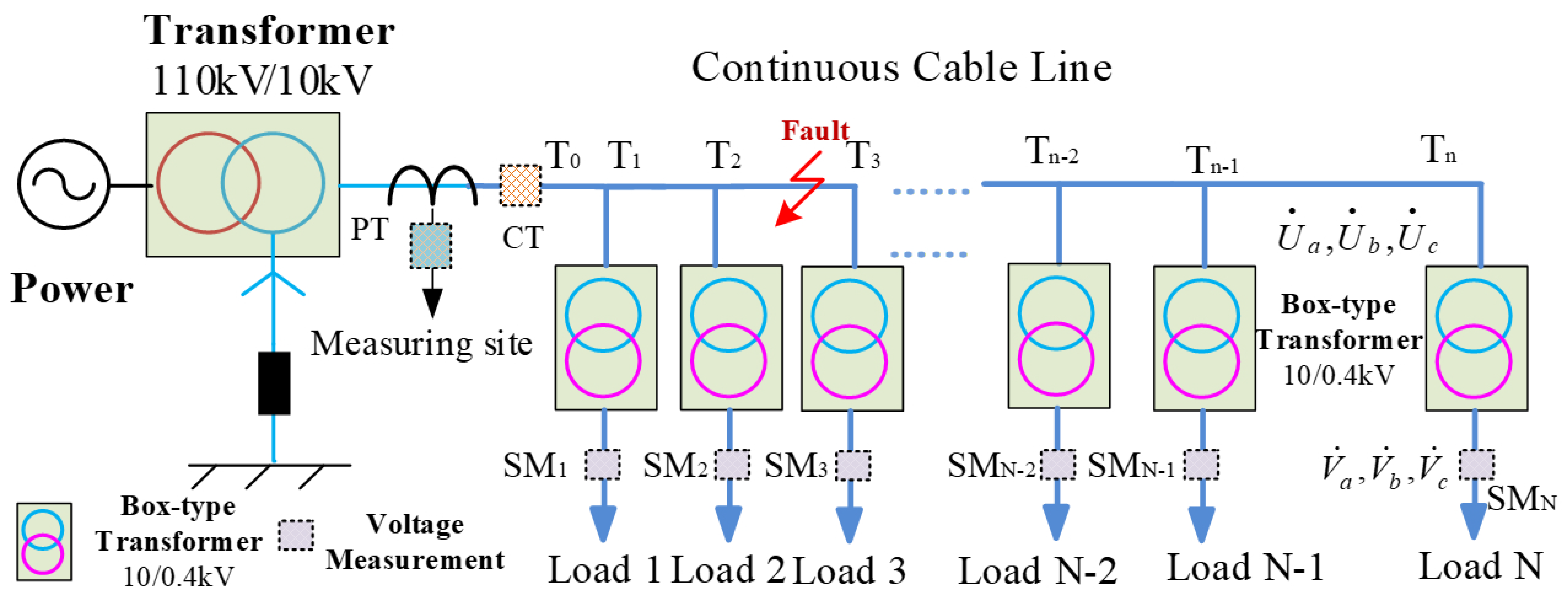
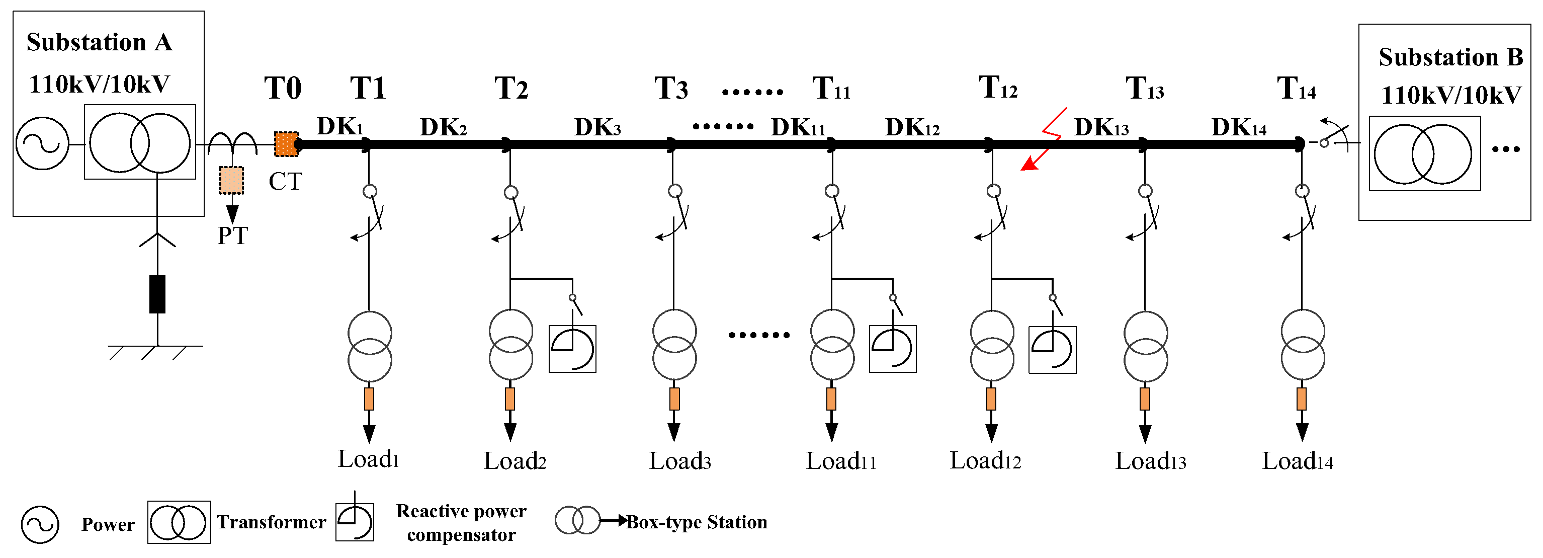
Compared with obtaining voltage signals from the high-voltage side (10 kV) of box-type substations, extracting voltage information from the low-voltage side (0.4 kV) presents distinct engineering advantages [20]. Voltage measurement on the high-voltage side generally requires dedicated voltage transformers. However, under operating conditions such as improper coordination of system parameters, switching over-voltages, or single-phase grounding, electromagnetic voltage transformers are prone to ferromagnetic resonance with the system-to-ground capacitance, which may further cause over-voltages, equipment damage, and even mal-operation of protective devices. In contrast, measuring voltage at the low-voltage terminals of box-type substations eliminates the need for additional high-voltage transformers, fundamentally reducing the excitation conditions of ferromagnetic resonance, and significantly improving the safety and reliability of high-speed railway distribution systems. Therefore, this section investigates the variation characteristics of voltage information obtained from low-voltage side measurements of box-type substations on continuous transmission lines. Figure 2 is the structure of the continuous transmission line [1]. Since the continuous transmission lines of high-speed railway adopt long cable lines, a low-resistance grounding system is applied to the neutral point. It should be noted that the neutral grounding mode affects the magnitude of ground fault current. The proposed method is derived from voltage and current at the substation inlet and line impedance parameters, so the neutral grounding resistance of the transformer is not included in the subsequent mathematical model.

Taking the typical connection mode of a box-type substation, Dyn11, as an example, the transfer characteristics of various voltage quantities are revealed, and the voltage relationship between the two sides of the transformer can be expressed:

$$\left[\begin{array}{c}{\dot{V}}_{\mathrm{a}}\\ {\dot{V}}_{\mathrm{b}}\\ {\dot{V}}_{\mathrm{c}}\end{array}\right]={\displaystyle \frac{1}{\sqrt{3}k}}\left[\begin{array}{ccc}1& -1& 0\\ 0& 1& -1\\ -1& 0& 1\end{array}\right]\left[\begin{array}{c}{\dot{U}}_{\mathrm{a}}\\ {\dot{U}}_{\mathrm{b}}\\ {\dot{U}}_{\mathrm{c}}\end{array}\right]$$

(1)

where, ${\dot{V}}_a,{\dot{V}}_b,{\dot{V}}_c$ are the three phase voltage at the low-voltage side of the box–type substation, respectively. ${\dot{U}}_a,{\dot{U}}_b,{\dot{U}}_c$ are the three phase voltage at the high-voltage side. k is the transformer factor. The relationship between sequence voltages and phase voltages is as follows:

$$\left[\begin{array}{c}{\dot{U}}_1\\ {\dot{U}}_2\\ {\dot{U}}_0\end{array}\right]={\displaystyle \frac{1}{3}}\left[\begin{array}{ccc}1& a& a^2\\ 1& a^2& a\\ 1& 1& 1\end{array}\right]\left[\begin{array}{c}{\dot{U}}_{\mathrm{a}}\\ {\dot{U}}_{\mathrm{b}}\\ {\dot{U}}_{\mathrm{c}}\end{array}\right]$$

(2)

${\dot{U}}_1,{\dot{U}}_2,{\dot{U}}_0$ are the positive, negative and zero sequence voltage at the 10 kV side of the box-type substation. a is the rotation factor. By combining the two formulas, the relationship between the sequence voltages on the high-voltage and low-voltage sides can be derived.

$$\left[\begin{array}{c}{\dot{V}}_1\\ {\dot{V}}_2\\ {\dot{V}}_0\end{array}\right]={\displaystyle \frac{1}{\sqrt{3}k}}\left[\begin{array}{ccc}{e}^{j{30}^{\circ }}& 0& 0\\ 0& e^{-{30}^{\circ }j}& 0\\ 0& 0& 0\end{array}\right]\left[\begin{array}{c}{\dot{U}}_1\\ {\dot{U}}_2\\ {\dot{U}}_0\end{array}\right]$$

(3)

${\dot{V}}_1,{\dot{V}}_2,{\dot{V}}_0$ are the positive, negative and zero-sequence voltages at the 0.4 kV side of the box-type substation.

2.2. The Characteristics of Positive and Negative Sequence Voltage Ratio

The positive and negative sequence voltage is defined as the characteristic quantity for fault location.

$$r_{PNV}={\displaystyle \frac{{\dot{V}}_1}{{\dot{V}}_2}}={\displaystyle \frac{e^{j{30}^{\circ }}{\dot{U}}_1}{e^{-j{30}^{\circ }}{\dot{U}}_2}}=e^{j{60}^{\circ }}{\displaystyle \frac{{\dot{U}}_1}{{\dot{U}}_2}}=e^{j{60}^{\circ }}{R}_{PNV}$$

(4)

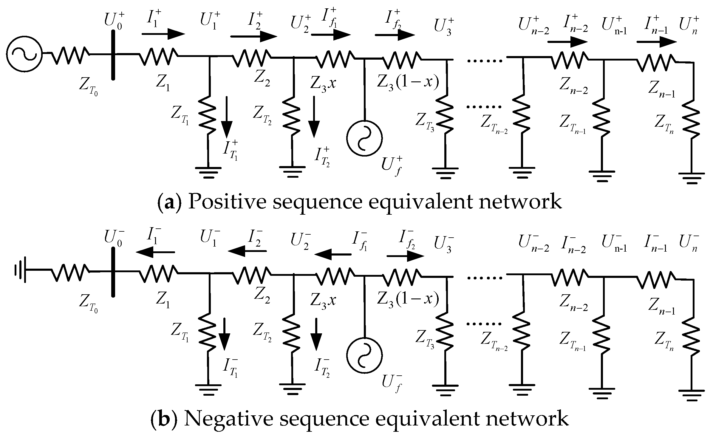
where, $r_{PNV}$ is the positive and negative sequence voltage ratio at the 0.4 kV side of the box-type substation. $R_{PNV}$ is the positive and negative sequence voltage ratio at the 10 kV side of the box-type substation. Since the defined characteristic quantity $r_{PNV}$ does not involve the zero-sequence network, Figure 3 shows the equivalent positive and negative sequence network under the assumption of a single-phase-to-ground fault occurring before node T₂ and node T₃.

The voltage and currents in the sequence network have been labeled in the figure. $\mathrm{Z}$ denotes the impedance of the section and ${\mathrm{Z}}_{\mathrm{T}}$ indicates the equivalent impedance of the transformer.

The voltages in the sequence network of fault downstream can be expressed in terms of the corresponding voltages at the fault point.

$$\left\{\begin{array}{l}{\dot{U}}_3^{+}={\dot{U}}_f^{+}-{\dot{I}}_{f2}^{+}·Z_3(1-x)\\ {\dot{U}}_4^{-}={\dot{U}}_f^{-}-{\dot{I}}_{f2}^{-}·Z_3(1-x)\end{array}\right.$$

(5)

where ${\dot{I}}_{f2}^{+}$ and ${\dot{I}}_{f2}^{-}$ can be expressed as follows:

$$\left\{\begin{array}{l}{\dot{I}}_{f2}^{+}={\displaystyle \frac{{\dot{U}}_3^{+}}{{\displaystyle \sum {\mathrm{Z}}_3}}}\\ {\dot{I}}_{f2}^{-}={\displaystyle \frac{{\dot{U}}_3^{-}}{{\displaystyle \sum {\mathrm{Z}}_3}}}\end{array}\right.$$

(6)

${\displaystyle \sum {\mathrm{Z}}_3}$ is the downstream equivalent impedance of node 3. Thus, by combining Equations (4) and (5), Equation (7) can be obtained.

$$\left\{\begin{array}{l}{\dot{U}}_f^{+}={\dot{U}}_3^{+}-{\displaystyle \frac{{\dot{U}}_3^{+}}{{\displaystyle \sum {\mathrm{Z}}_3}}}·Z_3(1-x)={\dot{U}}_3^{+}\left[1-{\displaystyle \frac{Z_3(1-x)}{{\displaystyle \sum {\mathrm{Z}}_3}}}\right]\\ {\dot{U}}_f^{-}={\dot{U}}_3^{-}-{\displaystyle \frac{{\dot{U}}_3^{-}}{{\displaystyle \sum {\mathrm{Z}}_3}}}·Z_3(1-x)={\dot{U}}_3^{-}\left[1-{\displaystyle \frac{Z_3(1-x)}{{\displaystyle \sum {\mathrm{Z}}_3}}}\right]\end{array}\right.$$

(7)

According to Equation (7), the relationship between the positive and negative sequence voltage ratio at the fault point and that at node 3 can be obtained, as shown in Equation (8).

$${\displaystyle \frac{{\dot{U}}_3^{+}}{{\dot{U}}_3^{-}}}={\displaystyle \frac{{\dot{U}}_f^{+}}{{\dot{U}}_f^{-}}}=R_{PNV3}=R_{PNVf}$$

(8)

Based on the structures shown in Figure 3, similar derivations can be used to obtain the relationships among node n−2, node n−1 and node n which are the nodes in the fault downstream.

$${\displaystyle \frac{{\dot{U}}_{n-2}^{+}}{{\dot{U}}_{\mathrm{n}-2}^{-}}}={\displaystyle \frac{{\dot{U}}_{fn-1}^{+}}{{\dot{U}}_{fn-1}^{-}}}={\displaystyle \frac{{\dot{U}}_n^{+}}{{\dot{U}}_n^{-}}}=R_{PNVn-2}=R_{PNVn-1}=R_{PNVn}$$

(9)

From Equation (4), we can derive the formula for the positive and negative sequence voltage ratio on the 0.4 kV side, as presented in Equation (10).

$$r_{PNV3}=\dots \dots =r_{PNVn}=r_{PNVf}=e^{j{60}^{\circ }}{R}_{PNVf}$$

(10)

Therefore, the actual value of $r_{PNVf}$ at the fault point can be expressed based on $r_{PNV}$ measured by the 0.4 kV side in the fault downstream. Meanwhile, $r_{PNV}$ at node belongs to the fault upstream can also be expressed. The formulas are shown in Equations (11) and (12).

$$r_{PNVf}=e^{j{60}^{\circ }}{\displaystyle \frac{{\dot{U}}_f^{+}}{{\dot{U}}_f^{-}}}=e^{j{60}^{\circ }}{\displaystyle \frac{{\dot{U}}_2^{+}-{\dot{I}}_{f_1}^{+}·Z_{3}x}{{\dot{U}}_2^{-}+{\dot{I}}_{f_1}^{-}·Z_{3}x}}$$

(11)

$$r_{PNV2}=e^{j{60}^{\circ }}{\displaystyle \frac{{\dot{U}}_2^{+}}{{\dot{U}}_2^{-}}}=e^{j{60}^{\circ }}{\displaystyle \frac{{\dot{U}}_1^{+}-{\dot{I}}_2^{+}·Z_2}{{\dot{U}}_1^{-}+{\dot{I}}_2^{-}·Z_2}}$$

(12)

According to Equations (11) and (12), the magnitude relationship expressed in Equation (13) can be obtained.

$$\left|r_{PNV1}\right|>\left|r_{PNV2}\right|>\left|r_{PNVf}\right|$$

(13)

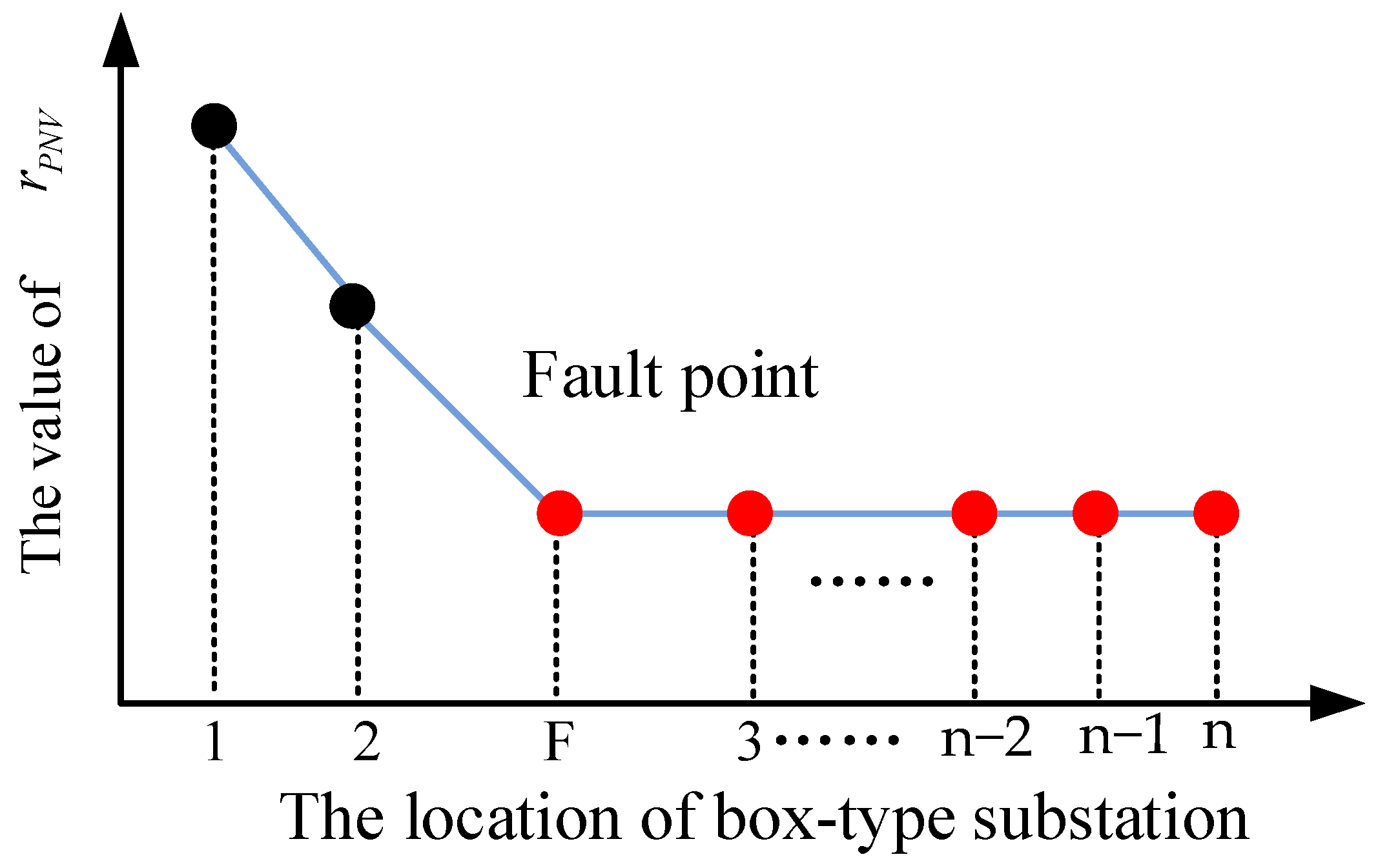
Therefore, the characteristics of the positive and negative sequence voltage ratio at the 0.4 kV side of the box-type substation at each node of the high-speed railway continuous transmission line are as follows. In the fault upstream, from the substation to the fault point, the magnitude of $r_{PNV}$ at each node decreases gradually. In the downstream of the fault, the magnitude of $r_{PNV}$ at each node is equal.

3. Implementation Process of Fault Section Identification and Fault Distance Calculation

High-speed railway continuous transmission lines are mainly composed of long-distance underground cables, whose total length usually exceeds tens of kilometers. Box-type substations are installed every several kilometers, and the overall structure is shown in Figure 2. For effective fault detection on these lines, fault section identification comes first, and the next step is to locate the specific fault point between two box-type substations. Targeting the real engineering setup of a local high-speed railway distribution system, this paper introduces the developed fault location method.

3.1. Fault Section Identification

As mentioned above, the basic principle of fault section identification is the ratio voltage distribution characteristics of sequence networks. According to the structure of the continuous transmission lines, ${\dot{V}}_a,{\dot{V}}_b,{\dot{V}}_c$ are the three phase voltage at 0.4 kV side of the box-type substation can be measured. Based on Equations (2) and (3), $r_{PNV}$ at each box-type substation node can be calculated. Assuming there is a fault between node 2 and node 3, the variation of the positive and negative sequence voltage ratio at each box-type substation node is shown in Figure 4.

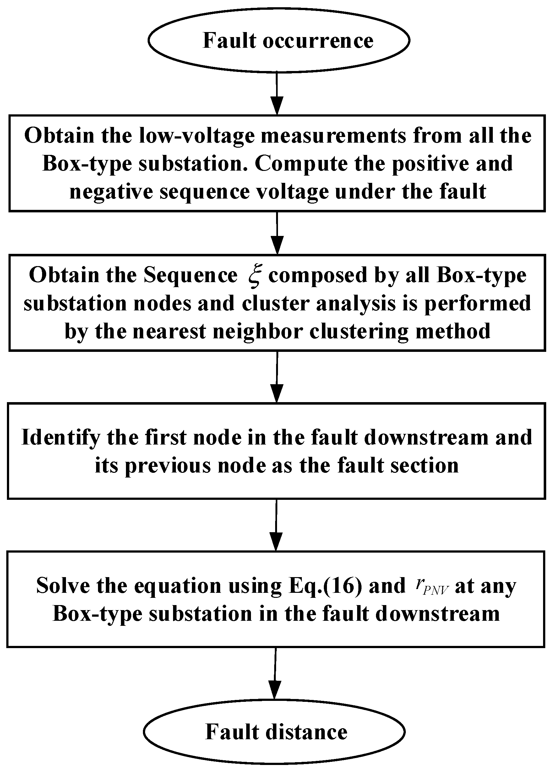
Therefore, the sequence $\xi$ can be obtained in Equation (14). In the sequence, the first box-type transformer node with the minimum value is successively identified as the end of the fault section, and the node with the second minimum value is taken as the beginning of the fault section.

$$\xi =\left[r_{PN{V}_1},r_{PN{V}_2},r_{PN{V}_3},\dots ,r_{PN{V}_{n-2}},r_{PN{V}_{n-1}},r_{PN{V}_n}\right]$$

(14)

Considering the interference of factors such as measurement errors, the $r_{PNV}$ in the downstream of the fault may not be completely consistent. In this paper, the nearest neighbor clustering method is used to cluster the values of Sequence $\xi$. Therefore, the node with the minimum value of $r_{PNV}$ can be selected in the cluster of the fault downstream. Assume that the Sequence $\xi$ with N data points has been obtained, the procedure of the improved nearest neighbor clustering method is as follows.

• Arbitrarily select data point $r_{PN{V}_i}(i=1,2,3,\dots ,N)$ as the initial value of the first cluster center, such as $C_1=r_{PN{V}_1}$.
• Calculate the distances form the N data points $\left[r_{PN{V}_1},r_{PN{V}_2},\dots \dots ,r_{PN{V}_{n-1}},r_{PN{V}_n}\right]$ to $C_1$, respectively. The distance set $\mathrm{D}=\left[D_1,D_2,\dots \dots ,D_{n-1},D_n\right]$ can be obtained. Where, $D_1=\left|r_{PN{V}_1}-C_1\right|/C_1$, $D_2=\left|r_{PN{V}_2}-C_2\right|/C_2$, …
• Identify all data corresponding to distances in set D that are smaller than the threshold $\theta$ and classify them into one cluster. Extract the data corresponding to distances large than $\theta$ from set D, repeat step (1) to define a new cluster center $C_2$, and then repeat step (2). This process is continued analogously until all N data points are classified.

3.2. Fault Distance Calculation

Once the fault is located between two box-type transformers, further fault distance calculation is required. Taking a fault that occurred between node 2 and node 3 as an example, ${\dot{U}}_2^{+}$ and ${\dot{U}}_2^{-}$ at the head end of the fault section can be derived from the fault upstream by Equation (15)

$${\displaystyle \frac{{\dot{U}}_2^{+}}{{\dot{U}}_2^{-}}}={\displaystyle \frac{{\dot{U}}_0^{+}-{\dot{I}}_1^{+}·Z_1-({\dot{I}}_1^{+}-({\dot{U}}_0^{+}-{\dot{I}}_1^{+}·Z_1)/Z_{T_1})·Z_2}{{\dot{U}}_0^{-}+{\dot{I}}_1^{-}·Z_1+({\dot{I}}_1^{-}+({\dot{U}}_0^{-}+{\dot{I}}_1^{-}·Z_1)/Z_{T_1})·Z_2}}$$

(15)

And then, the $r_{PNVf}$ of the fault point can also be derived from node 2 from the fault upstream by Equations (16)–(18).

$$r_{PNVf}=e^{j{60}^{\circ }}{\displaystyle \frac{{\dot{U}}_f^{+}}{{\dot{U}}_f^{-}}}=e^{j{60}^{\circ }}{\displaystyle \frac{{\dot{U}}_2^{+}-{\dot{I}}_{f_1}^{+}·Z_{3}x}{{\dot{U}}_2^{-}+{\dot{I}}_{f_1}^{-}·Z_{3}x}}=e^{j{60}^{\circ }}{\displaystyle \frac{{\dot{U}}_2^{+}-({\dot{I}}_2^{+}-{\dot{U}}_2^{+}/Z_{T_2})·Z_{3}x}{{\dot{U}}_2^{-}+({\dot{U}}_2^{-}/Z_{T_2}+{\dot{I}}_2^{-})·Z_{3}x}}$$

(16)

where,

$${\dot{I}}_2^{+}={\dot{I}}_1^{+}-{\displaystyle \frac{{\dot{U}}_1^{+}}{Z_{T_1}}}={\dot{I}}_1^{+}-{\displaystyle \frac{{\dot{U}}_0^{-}-{\dot{I}}_1^{+}{\mathrm{Z}}_1}{Z_{T_1}}}$$

(17)

$${\dot{I}}_2^{-}={\dot{I}}_1^{-}+{\displaystyle \frac{{\dot{U}}_1^{-}}{Z_{T_1}}}={\dot{I}}_1^{-}+{\displaystyle \frac{{\dot{U}}_0^{-}+{\dot{I}}_1^{-}{\mathrm{Z}}_1}{Z_{T_1}}}$$

(18)

As shown in Equation (16), the positive and negative sequence voltage ratio at the 0.4 kV side of the box-type substation is a function related to fault distance x. where, ${\dot{U}}_0^{+}$, ${\dot{U}}_0^{-}$, ${\dot{I}}_1^{+}$, ${\dot{I}}_1^{-}$ can be calculated by three-phase voltage and current of the head-end substation. Because the value of $r_{PNVf}$ can be obtained by low-voltage measurements at a box-type substation in the fault downstream, the fault distance x can be solved by Equations (15)–(18).

3.3. The Detailed Process of the Proposed Fault Location

The proposed method involves two main procedures. One is fault section identification, and the other is fault distance calculation. The key characteristic parameter is the positive and negative sequence voltage ratio at the 0.4 kV side of the box-type substation. When an asymmetric fault occurs on the high-speed railway continuous transmission lines, the location process can be initiated by zero-sequence or negative-sequence threshold detection. Firstly, collect the three-phase voltages on the 0.4 kV side of each box-type substation node along the continuous transmission lines and calculate the positive and negative sequence voltage ratios $r_{PNV}$. Secondly, construct the sequence $\xi$ composed of each box-type substation node. The nearest neighbor clustering is employed to cluster the ratio $r_{PNV}$ in the sequence, and obtain the set of nodes in the fault downstream with the minimum ratio value. Then, identify the first node in the fault downstream and its previous node as the fault section. Finally, using the voltage and current information at the 10 kV main substation, the voltage and current at the head end of the fault section are calculated based on the topology and parameters of the fault upstream. Establish the equation between the fault distance and the ratio $r_{PNVf}$. Select the ratio $r_{PNV}$ of any node in the fault downstream as the ratio value of the fault point, substitute it into the equation and solve to obtain the fault distance result. After data acquisition, the overall fault location algorithm completes the calculation within 3 s, exhibiting favorable timeliness. The flow chart of the fault section identification and fault distance estimation is shown in Figure 5.

4. Simulation Verification

To validate the feasibility and accuracy of the proposed fault localization strategy, simulation tests are carried out based on a practical 10 kV continuous transmission line belonging to China’s high-speed railway power distribution system. The core parameters of the experimental platform and test system are summarized in

Table 1. The parameters of the tested continuous transmission lines based on the Zhong Shan Xi Station [1].

Section	DK1	DK2	DK3	DK4	DK5	DK6	DK7
Length (km)	0.023	3.994	3.446	2.023	1.511	2.732	0.495
Section	DK8	DK9	DK10	DK11	DK12	DK13	DK14
Length (km)	2.217	2.762	2.148	2.248	2.699	2.519	2.7428

. In this work, the PSCAD/EMTDC 4.6.2 simulation software is adopted to establish the full-scale power network model, which can acquire complete operating data of substations under normal operation and fault conditions. Meanwhile, the algorithm model of the novel fault location scheme is programmed and built on the MATLAB R2019a platform. By importing the high-precision simulation data obtained from the PSCAD/EMTDC model, the designed algorithm can realize intelligent identification and quantitative calculation of fault positions. In addition, the positioning accuracy of the proposed approach is assessed via the relative error formula, as defined in Equation (19). where, $x_r$ is the actual fault distance and $x_e$ is the calculated fault distance.

$$E_{relative}={\displaystyle \frac{\left|x_r-x_e\right|}{x_r}}$$

(19)

The schematic diagram of the tested continuous transmission lines based on the Zhong Shan Xi Station is shown in Figure 6. The tests were conducted considering single-phase-to-ground faults, two-phase-to-ground faults, and two-phase faults. In order to demonstrate the application of the proposed method, the sampling frequency of smart meters was set to 800 Hz in the box-type substation.

4.1. Method Effectiveness Analysis

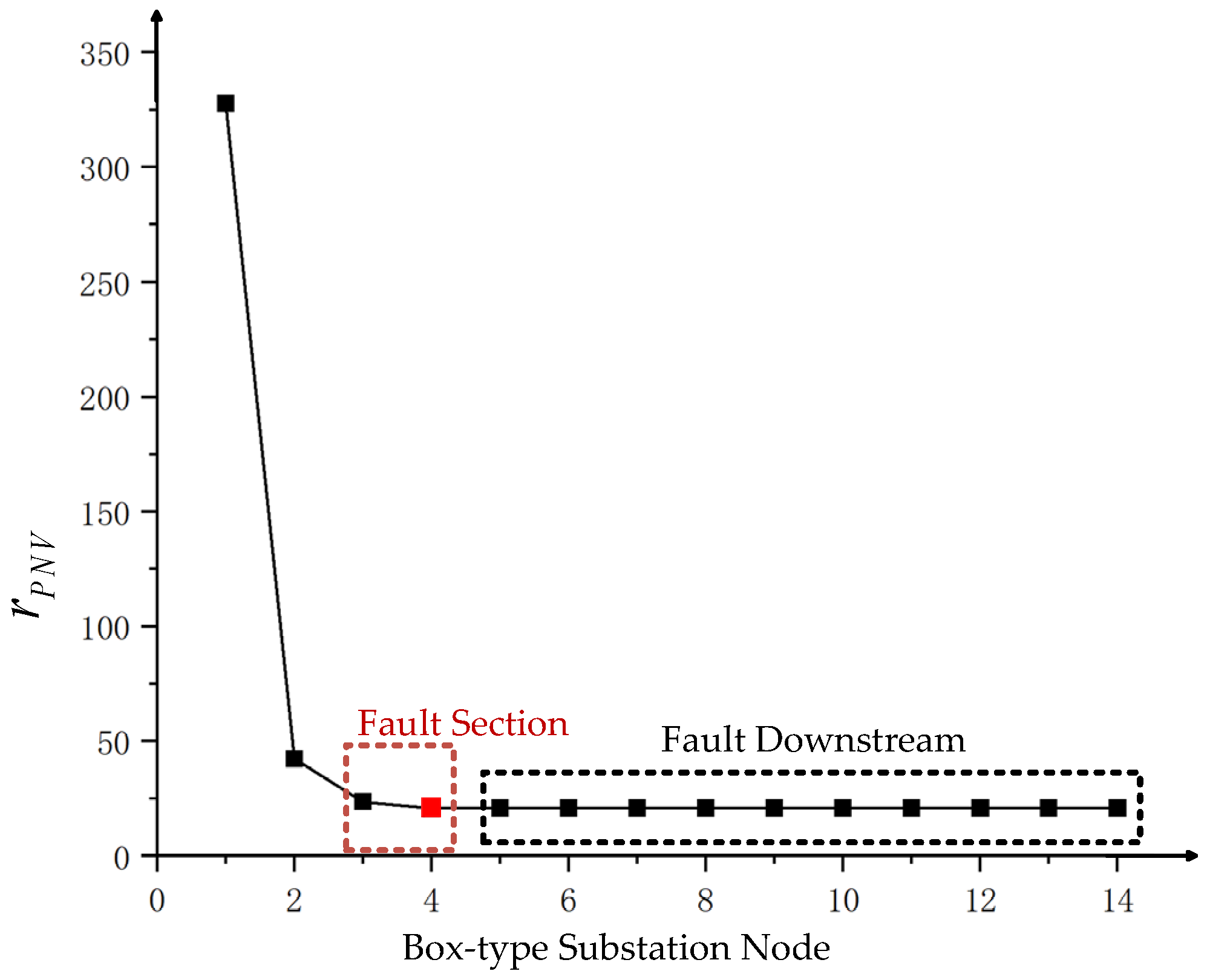
Taking a single-phase grounding fault at the midpoint of section DK₄ as an example, with a fault resistance of 10Ω. The low-voltage measurements from all the box-type substations are analyzed. By calculating the ratio of the sequence voltages during the fault, the sequence $\xi$ is [327.9, 42.4, 23.6, 20.8, 20.8, 20.8, 20.8, 20.8, 20.8, 20.8, 20.8, 20.8, 20.8, 20.8]. The minimum value is 20.8. Setting the threshold at 5%, the clustering range is determined to be 19.76 to 21.84. Consequently, the section location result is shown in Figure 7.

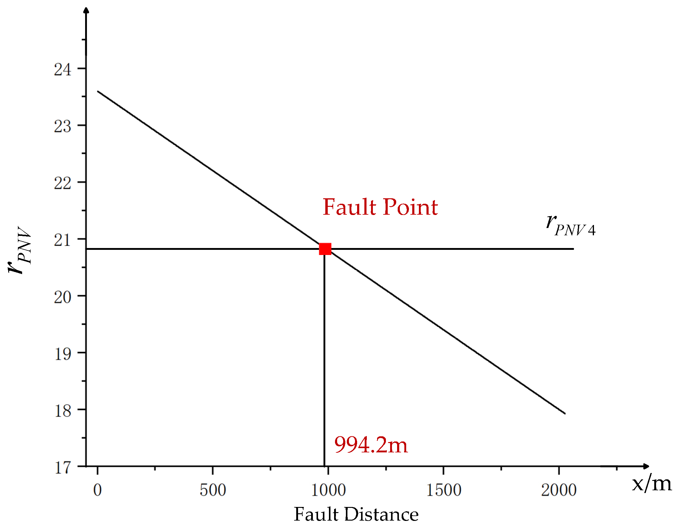
It can be observed that the fault occurred between Section T₃ and T₄. Furthermore, by using the voltage and current from the beginning of DK₄ and the measurements from any box-type substation node in the fault downstream, the calculated fault position is 994.2 m, as shown in Figure 8.

The value of $E_{absolute}$ and $E_{relative}$ are 17.3 m and 1.7%, respectively. This demonstrates that the proposed method achieves an accurate fault location.

4.2. Method Sensitivity to the Fault Resistance

To validate the method’s sensitivity to fault resistance, fault location was performed for faults occurring at the midpoints of sections DK₂ and DK₈, respectively. A phase-A grounding fault with a small-resistance grounded mode is considered, where the fault resistance ranges from 1 Ω to 2000 Ω. The obtained location results are shown in

Table 2. The result of fault location under different fault impedance.

Fault Section	Fault Resistance	The Sequence $\mathit{\xi }$	Fault Section	Distance	${\mathit{E}}_{\mathit{r}\mathit{e}\mathit{l}\mathit{a}\mathit{t}\mathit{i}\mathit{v}\mathit{e}}$
DK2	1	[52.3 11.6 11.6 11.6 11.6 11.6 11.6 11.6 11.6 11.6 11.6 11.6 11.6 11.6]	DK2	1.9880	0.5%
	10	[248.8 58.2 58.2 58.2 58.2 58.2 58.2 58.2 58.2 58.2 58.2 58.2 58.2 58.2]	DK2	1.9890	0.4%
	100	[2352.9 556.2 556.2 555.9 555.9 555.6 555.6 555.6 555.6 555.2 555.2 555.2 555.2 555.2]	DK2	1.9900	0.4%
	500	[11,723.3 2765.5 2760.1 2756.3 2751.8 2748.8 2748.8 2746.5 2743.5 2742.0 2740.5 2739.7 2739.0 2738.2]	DK2	1.9959	0.1%
	2000	[46,794.6 10,949.3 10,864.8 10,803.8 10,741.1 10,689.5 10,691.8 10,651.9 10,615.7 10,587.6 10,565.2 10,548.5 10,539.6 10,535.2]	DK2	2.0180	1.1%
DK8	1	[320.5 41.7 23.3 18.4 15.8 12.6 12.2 11.3 11.3 11.3 11.3 11.3 11.3 11.3]	DK8	1.0940	1.3%
	10	[438.6 57.7 32.4 25.6 22.1 17.6 17.0 15.8 15.8 15.8 15.8 15.8 15.8 15.8]	DK8	1.0960	1.1%
	100	[2500.0 326.8 184.5 146.8 127.2 102.6 99.0 92.0 92.0 92.0 92.0 92.0 92.0 92.0]	DK8	1.0989	0.9%
	500	[11,904.8 1574.8 892.1 710.2 615.8 497.0 480.1 446.0 446.0 446.0 446.0 446.0 446.0 446.0]	DK8	1.1082	0.03%
	2000	[47,393.4 6238.3 3533.6 2813.7 2439.6 1969.3 1903.3 1768.0 1767.1 1766.5 1765.8 1765.5 1765.2 1765.2]	DK8	1.1435	3.2%

. In the table, the bold values represent nodes clustered as fault downstream.

From the fault location data summarized in Table 2, it is observed that favorable accuracy in fault identification and distance estimation can be guaranteed under all tested fault resistances, including high-resistance fault scenarios. The above results verify the strong sensitivity of the proposed scheme toward fault resistance.

4.3. Method Sensitivity to the Fault Type

To verify the method’s sensitivity to fault types, fault location was performed for faults occurring at the midpoints of sections DK₄ and DK₁₀, respectively. The fault resistance was set to 10Ω, with small resistance grounded mode, and the fault types included single-phase-to-ground fault on phase A (Ag), phase-to-phase short-circuit fault between phases B and C (BC), and double-phase-to-ground short-circuit fault on phases B and C (BCg). The obtained location results are presented in

Table 3. The result of fault location under different fault types.

Fault Section	Fault Type	The Sequence $\mathit{\xi }$	Fault Section	Distance	${\mathit{E}}_{\mathit{r}\mathit{e}\mathit{l}\mathit{a}\mathit{t}\mathit{i}\mathit{v}\mathit{e}}$
DK4	Ag	[327.9 42.4 23.6 20.8 20.8 20.8 20.8 20.8 20.8 20.8 20.8 20.8 20.8 20.8]	DK4	0.9940	1.7%
	BC	[100.0 13.0 6.9 6.1 6.1 6.1 6.1 6.1 6.1 6.1 6.1 6.1 6.1 6.1]	DK4	0.9890	2.2%
	BCg	[215.5 27.3 14.9 13.1 13.1 13.1 13.1 13.1 13.1 13.1 13.1 13.1 13.1 13.1]	DK4	0.9880	2.3%
DK10	Ag	[534.8 70.0 39.2 31.1 26.8 21.5 20.7 17.9 15.2 14.4 14.4 14.4 14.4 14.4]	DK10	1.0768	0.3%
	BC	[142.9 17.9 9.8 7.6 6.5 5.0 4.8 4.1 3.4 3.1 3.1 3.1 3.1 3.1]	DK10	1.0776	0.3%
	BCg	[250.0 30.3 16.7 13.2 11.2 8.8 8.5 7.3 6.1 5.7 5.7 5.7 5.7 5.7]	DK10	1.0746	0.1%

.

The data presented in Table 3 reveal that this approach maintains reliable positioning and distance calculation accuracy when handling various fault categories. The results verify that the developed algorithm is well adaptable to different fault types.

4.4. Result of Signals with Noise

To verify the impact of signal noise, fault location was performed for faults occurring at the midpoints of sections DK₅ and DK₉, respectively. The fault type is set as BCg, with a small-resistance grounded mode at the neutral point and a fault resistance of 10 Ω. Verification was conducted under three scenarios: signals without noise, signals with measurement errors within 0.52% due to noise, and signals with phase shifts within one cycle caused by noise. Ten sets of experiments were conducted for each scenario, and the average value was taken as the fault distance measurement result, as shown in

Table 4. The location result of signals with noise.

Fault Section	Measurement Errors or Synchronization	Fault Section	Average Distance (km)	${\mathit{E}}_{\mathit{r}\mathit{e}\mathit{l}\mathit{a}\mathit{t}\mathit{i}\mathit{v}\mathit{e}}$	Standard Deviation	Maximum Error (km)
DK5	Measurement error within 0.52% [21]	DK5	0.7378	2.4%	1.31 × 10−2	0.045
	Random phase shift within 1 cycle	DK5	0.7361	2.6%	1.66 × 10−4	0.019
DK9	Measurement error within 0.52% [21]	DK9	1.3743	0.5%	1.11 × 10−2	0.038
	Random phase shift within 1 cycle	DK9	1.3732	0.6%	1.18 × 10−4	7.95 × 10−3

. As shown in Table 4, the maximum error of the fault distance with measurement errors or synchronization is within 50 m.

Table 4 summarizes the fault location outcomes under multiple noise environments. It is clear that the devised technique sustains high precision in fault positioning and distance computation. These findings prove that the method has strong resistance against signal noise interference.

4.5. Result of Different Neutral Grounding Mode

To verify the method’s sensitivity to the neutral grounding mode, fault location is performed for faults occurring at the midpoints of sections DK₆ and DK₁₁, respectively. The fault resistance is 10 Ω, the fault type is Ag, and the neutral grounding modes are the small resistance grounded mode (SR-grounded), ungrounded mode, and resonant grounded mode (R-grounded). The obtained location results are shown in

Table 5. The result of fault location under different neutral grounding modes.

Fault Section	Neutral Grounding Mode	The Sequence $\mathit{\xi }$	Fault Section	Distance	${\mathit{E}}_{\mathit{r}\mathit{e}\mathit{l}\mathit{a}\mathit{t}\mathit{i}\mathit{v}\mathit{e}}$
DK6	SR-grounded	[613.5 80.0 44.9 35.6 30.7 27.3 27.3 27.3 27.3 27.3 27.3 27.3 27.3 27.3]	DK6	1.3486	1.3%
	Ungrounded	[2487.6 328.8 186.5 148.7 129.0 115.3 115.3 115.3 115.3 115.3 115.3 115.3 115.3 115.3]	DK6	1.3460	1.5%
	R-grounded	[1639.3 217.0 122.5 97.4 84.4 75.3 75.3 75.3 75.3 75.3 75.3 75.3 75.3 75.3]	DK6	1.3497	1.2%
DK11	SR-grounded	[1923.1 255.8 144.3 114.8 99.5 80.1 77.4 67.1 57.5 51.7 49.1 49.1 49.1 49.1]	DK11	1.1575	3.0%
	Ungrounded	[769.2 101.0 56.8 45.0 38.9 31.2 30.1 26.0 22.2 19.9 18.9 18.9 18.9 18.9]	DK11	1.1556	2.8%
	R-grounded	[2439.0 325.7 184.8 147.5 128.0 103.4 100.0 86.8 74.6 67.3 64.0 64.0 64.0 64.0]	DK11	1.1517	2.5%

.

Table 5 records the test results under various neutral grounding modes. The proposed method retains high precision in fault section and distance calculation across different operating modes. This confirms that the approach works well with diverse neutral grounding schemes.

4.6. Result of Missing Measurement Data

Table 6. The result of fault location with missing measurement data.

Fault Section	Missing Data	The Sequence $\mathit{\xi }$	Fault Section	Distance (km)	${\mathit{E}}_{\mathit{r}\mathit{e}\mathit{l}\mathit{a}\mathit{t}\mathit{i}\mathit{v}\mathit{e}}$
DK6	Case1: L1, L13	[28.1 15.4 12.0 10.3 9.0 9.0 9.0 9.0 9.0 9.0 9.0 9.0]	DK6	1.3404	1.9%
	Case2: L1, L3, L13	[28.1 12.0 10.3 9.0 9.0 9.0 9.0 9.0 9.0 9.0 9.0]	DK6	1.3404	1.9%
	Case3: L1, L3, L6, L8, L13	[28.1 12.0 10.3 9.0 9.0 9.0 9.0 9.0 9.0]	DK6-DK7	1.3404	1.9%
	Case4: L1, L3, L5, L6, L10, L13	[28.1 12.0 9.0 9.0 9.0 9.0 9.0 9.0]	DK5-DK7	2.8515	0.9%

presents the scenarios of missing measurement points at different locations after a fault occurs on DK₆. It can be seen that accurate fault section and fault location can be obtained as long as no measurements are missing in the fault section, as demonstrated in Case 1 and Case 2. If measurements within the fault section are lost, as shown in Case 3 and Case 4, the fault section identification result depends on the range of missing data. Meanwhile, the fault location result remains unaffected, provided that there is at least one measurement point downstream of the fault.

4.7. Result of Load Variation

Table 7. Influence of load variation on fault localization results.

Fault Section	Load Fluctuation	The Sequence $\mathit{\xi }$	Fault Section	Distance (km)	${\mathit{E}}_{\mathit{r}\mathit{e}\mathit{l}\mathit{a}\mathit{t}\mathit{i}\mathit{v}\mathit{e}}$
DK5	No Fluctuation	[377.2 49.0 27.3 21.6 19.9 19.9 19.9 19.9 19.9 19.9 19.9 19.9 19.9 19.9]	DK5	0.7391	2.2%
	10%	[377.7 49.0 27.3 21.6 20.0 20.0 20.0 20.0 20.0 20.0 20.0 20.0 20.0 20.0]	DK5	0.7382	2.3%
	20%	[378.3 49.1 27.4 21.6 20.0 20.0 20.0 20.0 20.0 20.0 20.0 20.0 20.0 20.0]	DK5	0.7373	2.4%

presents the scenarios of load variation after a fault occurs on DK₅. As shown in Table 7, load deviation has little effect on fault localization results. The main reason is that the positive and negative sequence voltage ratio defined in this paper can eliminate the influences of line topology and loads in the downstream of the fault. Therefore, the proposed algorithm presents good adaptability to load deviation.

4.8. Result of Cable Parameter Errors

Table 8. Influence of cable parameter errors on fault localization results.

Fault Section	Line Parameter Error	The Sequence $\mathit{\xi }$	Fault Section	Distance (km)	${\mathit{E}}_{\mathit{r}\mathit{e}\mathit{l}\mathit{a}\mathit{t}\mathit{i}\mathit{v}\mathit{e}}$
DK4	1%	[215.3 27.3 14.9 13.1 13.1 13.1 13.1 13.1 13.1 13.1 13.1 13.1 13.1 13.1]	DK4	1.0731	6.1%
	2%	[215.3 27.3 14.9 13.1 13.1 13.1 13.1 13.1 13.1 13.1 13.1 13.1 13.1 13.1]	DK4	1.1603	14.7%

presents the scenarios of cable parameter errors after the BC-phase earth fault occurred in DK₄. The location results are analyzed under impedance parameter errors of 1% and 2%. As shown in Table 8, the fault section identification does not involve line parameters, so it is immune to cable parameter errors. However, the fault distance relies on accurate per-unit impedance parameters, and thus parameter errors will impose certain impacts on the results. As the parameter error increases, the error of fault distance rises gradually. Therefore, we can update line parameters via online identification and other methods to ensure the accuracy of basic line data.

4.9. Comparison Results with Existing Methods

This section compares the proposed method with the impedance-based method [3], the voltage sag-based method [1] and the low-voltage measurement-based method [2,20], and the results are presented in

Table 9. Comparative analysis results of different fault location methods.

Method Types	Reference	Measurement Requirements		Accuracy		Fault Condition
		Synchronization	Voltage Level	Distance Estimation	Distance Error	Fault Resistance
Low-voltage Measurement-based	Proposed method	No	0.4 kV	Yes	<100 m	<2000 Ω
	[2]	Yes	0.4 kV	Yes	<150 m	<100 Ω
	[20]	No	0.4 kV	Yes	<200 m	<2000 Ω
Impedance-based	[3]	Yes	20 kV	Yes	<100 m	<100 Ω
Voltage Sag-based	[1]	Yes	10 kV	Yes	<100 m	<10 Ω

. As shown in Table 9, the impedance-based method is greatly affected by fault resistance, and only performs well for faults with transition resistance within 100 Ω. Compared with the low-voltage measurement method, the proposed method shows advantages in high-resistance fault identification and ranging accuracy.

4.10. Discussion

This section analyzes the limitations of the proposed algorithm under two operating conditions: communication interruption and network topology variation. The algorithm heavily relies on measurement data uploaded from box-type transformers, so the reliability of communication links at measurement points is critical to its operation. In case of communication failure, the adverse impact on algorithm performance can be analyzed by analogy with the scenario of missing measurement data presented in Section 4.6. With regard to topology variation, high-speed railway continuous transmission lines generally feature a relatively fixed topological configuration, and the structure of backup lines is identical to that of main lines, resulting in rare topology adjustments in practical operation. Nevertheless, as large-scale new energy will be continuously connected to high-speed railway distribution systems, dynamic topology changes will become an inevitable operational challenge, which requires in-depth targeted research. In addition, validating the algorithm with field-measured data from FTUs and RTUs is also an important direction for future research.

5. Conclusions

This paper presents an accurate fault location method for high-speed railway continuous transmission lines based on low-voltage measurements from box–type substations. The core of the method is to utilize the unique distribution characteristics of the positive and negative sequence voltage ratio along continuous transmission lines during asymmetric faults.

The proposed method operates in two stages: fault section identification and precise distance calculation. The fault section is identified by analyzing the sequence of positive and negative sequence voltage ratio values collected from all box-type substations and adopting the nearest-neighbor clustering algorithm to acquire downstream fault nodes. The fault position is then calculated by solving equations that correlate the positive and negative sequence voltage ratio at the fault point with measured data from the main substation and downstream box-type substations.

Comprehensive case studies validate the method’s effectiveness. It can accurately identify various fault types and maintains high reliability under high fault resistance (up to 2000 Ω), different neutral earthing modes, actual measurement noise and phase shift errors. It is worth noting that the fault distance calculation in the second stage relies on accurate line impedance. Therefore, further research will focus on line parameter identification based on monitoring units to enhance the robustness of the algorithm against parameter deviations.

References

1. Zhang, S.; He, Z.; Lee, W.; Mai, R. Voltage Sag Profiles Based Fault Location in High Speed Railway Distribution System. IEEE Trans. Ind. Appl. 2017, 5, 5229–5238. [Google Scholar] [CrossRef]
2. Buzo, R.F.; Barradas, H.M.; Leao, F.B. A New Method for Fault Location in Distribution Networks Based on Voltage Sag Measurements. IEEE Trans. Power Deliv. 2021, 36, 651–662. [Google Scholar] [CrossRef] [Scilit]
3. Mirshekali, H.; Dashti, R.; Keshavarz, A.; Torabi, A.J.; Shaker, H.R. A Novel Fault Location Methodology for Smart Distribution Networks. IEEE Trans. Smart Grid 2021, 12, 1277–1288. [Google Scholar] [CrossRef] [Scilit]
4. Gao, L.M.; Liu, B.; Gao, F.; Chen, J. Fault Location Algorithm in Distribution Networks Considering Distributed Capacitive Current. IEEE Trans. Power Deliv. 2021, 36, 2785–2793. [Google Scholar] [CrossRef] [Scilit]
5. Gholami, M.; Abbaspour, A.; Moeini-Aghtaie, M.; Fotuhi-Firuzabad, M.; Lehtonen, M. Detecting the Location of Short-Circuit Faults in Active Distribution Network Using PMU-Based State Estimation. IEEE Trans. Smart Grid 2020, 11, 1396–1406. [Google Scholar] [CrossRef] [Scilit]
6. Pang, Q.; Wang, Y.; Wang, Y.; Cao, T. Earth Fault Location for Non-Directly Grounded Distribution Networks. IEEE Trans. Power Deliv. 2024, 39, 706–717. [Google Scholar] [CrossRef] [Scilit]
7. Zhou, J.; Ayhan, B.; Kwan, C.; Liang, S.; Lee, W. High-Performance Arcing-Fault Location in Distribution Networks. IEEE Trans. Ind. Appl. 2012, 48, 1107–1114. [Google Scholar] [CrossRef] [Scilit]
8. Sodin, D.; Smolnikar, M.; Rudež, U.; Čampa, A. Precise PMU-Based Localization and Classification of Short-Circuit Faults in Power Distribution Systems. IEEE Trans. Power Deliv. 2023, 38, 3262–3273. [Google Scholar] [CrossRef] [Scilit]
9. Yun, Z.; Wen, T.; Wang, C. Fault Location Method for Three-Terminal Lines in Distribution Network Based on Line Voltage Measured by μ MPMU. IEEE Trans. Smart Grid 2021, 12, 5095–5112. [Google Scholar] [CrossRef] [Scilit]
10. Lin, J.; Guo, M.; Zheng, Z. Active Location Method for Single-Line-to-Ground Fault of Flexible Grounding Distribution Networks. IEEE Trans. Instrum. Meas. 2023, 72, 3524712. [Google Scholar]
11. Lin, J.; Guo, M.; Hong, Q.; Jiang, R. An Earth Fault Diagnosis Method Based on Online Dynamically Calculated Thresholds for Resonant Ground Systems. IEEE Trans. Smart Grid 2024, 15, 3459–3473. [Google Scholar] [CrossRef] [Scilit]
12. Guo, M.; Gao, J.; Shao, X.; Chen, D. Location of Single-Line-to-Ground Fault Using 1-D Convolutional Neural Network and Waveform Concatenation in Resonant Grounding Distribution Systems. IEEE Trans. Instrum. Meas. 2021, 70, 3501009. [Google Scholar] [CrossRef] [Scilit]
13. MansourLakouraj, M.; Hosseinpour, H.; Livani, H.; Benidris, M. Waveform Measurement Unit-Based Fault Location in Distribution Feeders via Short-Time Matrix Pencil Method and Graph Neural Network. IEEE Trans. Ind. Appl. 2023, 59, 2661–2670. [Google Scholar] [CrossRef] [Scilit]
14. Lv, X.; Yuan, L.; Cheng, Z.; Zuo, L.; Yin, B.; He, Y.; Ding, C. An Improved Bayesian Learning Method for Distribution Grid Fault Location and Meter Deployment Optimization. IEEE Trans. Instrum. Meas. 2024, 73, 3519910. [Google Scholar] [CrossRef] [Scilit]
15. Shan, H.T.; Wu, Q.H.; Li, C.T.; Zhang, L.L. Sparse Over-complete Representation Fault Location Model in Distribution Networks and Efficient Solution Using Fast Laplace Bayesian. IEEE Trans. Instrum. Meas. 2024, 73, 3517311. [Google Scholar] [CrossRef] [Scilit]
16. Jiang, K.; Wang, H.; Shahidehpour, M.; He, B. Block-Sparse Bayesian Learning Method for Fault Location in Active Distribution Networks with Limited Synchronized Measurements. IEEE Trans. Power Syst. 2021, 36, 3189–3203. [Google Scholar] [CrossRef] [Scilit]
17. Pereira, R.A.; Da Silva, L.G.; Kezunovic, M.; Mantovani, J.R. Location of single line-to-ground on distribution feeders using voltage Measurements. In Proceedings of the 2006 IEEE/PES Transmission & Distribution Conference and Expositon: Latin America, Caracas, Venezuela, 15–18 August 2006. [Google Scholar]
18. Lotfifard, S.; Kezunovic, M.; Mousavi, M.J. Voltage sag data utilization for distribution fault location. IEEE Trans. Power Deliv. 2011, 2, 1239–1246. [Google Scholar] [CrossRef] [Scilit]
19. Brahma, S.M. Fault Location in Power Distribution System with Penetration of Distributed Generation. IEEE Trans. Power Deliv. 2011, 3, 1545–1553. [Google Scholar] [CrossRef] [Scilit]
20. Zhang, S.; Chen, H.; Tang, J.; Zhang, W.; Zang, T.; Xiao, X. Fault Location Based on Voltage Measurement at Secondary Side of Low-Voltage Transformer in Distribution Network. IEEE Trans. Instrum. Meas. 2022, 71, 3522512. [Google Scholar] [CrossRef] [Scilit]
21. Std IEEE C37.242-2021; IEEE Guide for Synchronization, Calibration, Testing, and Installation of Phasor Measurement Units (PMUs) for Power System Protection and Control. IEEE: Piscataway, NJ, USA, 2021.
Figure 1. Configuration of the high-speed railway continuous transmission lines.
Energies 19 02974 g001
Figure 2. The structure of the continuous transmission lines.
Energies 19 02974 g002
Figure 3. Positive and negative sequence network with a single-phase-to-ground fault.
Energies 19 02974 g003
Figure 4. Schematic diagram of the r P N V at each box-type substation node.
Energies 19 02974 g004
Figure 5. The flow chart of the fault section identification and fault distance estimation.
Energies 19 02974 g005
Figure 6. The tested continuous transmission lines based on the Zhong Shan Xi Station.
Energies 19 02974 g006
Figure 7. Schematic diagram of the r P N V at each box-type substation node.
Energies 19 02974 g007
Figure 8. Schematic diagram of the r P N V at each box-type substation node.
Energies 19 02974 g008