Article

Research on the Comprehensive Energy Management Model for Ports with Land-Based Traffic Consideration


1
School of Economics and Management, Shanghai University of Political Science and Law, Shanghai 201701, China
2
China Institute of FTZ Supply Chain, Shanghai Maritime University, Shanghai 201306, China
3
Public Experiment Center, University of Shanghai for Science and Technology, Shanghai 200093, China
*
Author to whom correspondence should be addressed.
Energies 2026, 19(13), 2970; https://doi.org/10.3390/en19132970
Submission received: 13 May 2026 / Revised: 4 June 2026 / Accepted: 18 June 2026 / Published: 24 June 2026

Abstract

Port operators must now reduce emissions without weakening the reliability of cargo-handling and logistics services. Two load groups are especially important in this setting: vessels connected to shore-side facilities during berthing and heavy-duty vehicles working inside the terminal area. Their energy-use patterns shape both dispatch stability and the carbon intensity of the port energy system. This paper therefore proposes an integrated port energy management model that jointly schedules wind power, photovoltaic generation, hydrogen production and storage, shore power, conventional purchases, berthed-vessel demand, and low-carbon heavy-duty transport demand. The model combines price-based demand response with a tiered carbon-trading penalty so that flexible electricity consumption and emission costs are reflected in the dispatch decision. Numerical simulations show that the joint use of demand response and the carbon-penalty mechanism lowers total economic dispatch cost by about 11.05 % and reduces carbon emissions by 24.52 % . The results indicate that coordinated renewable-energy and logistics-aware scheduling can improve the economic and environmental performance of port operations.

1. Introduction

Ports connect maritime transport with inland distribution and regional production, yet their daily operation consumes large amounts of electricity, heat, and fuel. Under carbon-peaking and carbon-neutrality targets, terminals must keep cargo throughput stable while replacing high-emission energy use with cleaner and more flexible supply. This transition requires more on-site renewable generation, tighter coordination between logistics loads and energy assets, and explicit attention to ship and vehicle energy demand. As wind power, photovoltaic generation, hydrogen, shore-power, and storage technologies become increasingly deployable in port areas, integrated scheduling can link logistics activity with multi-carrier energy operation. A coordinated management framework is therefore important for improving energy efficiency, cutting emissions, and supporting the green transformation of port systems [1].
An integrated port energy system contains two tightly connected layers. The energy layer purchases, converts, stores, and supplies several energy carriers for terminal production and auxiliary services [2]. The logistics layer determines the timing and intensity of cargo handling, berthing, loading and unloading, and vehicle movements, thereby creating highly variable demand. In the framework developed here, grid electricity and fossil-fuel purchases remain available for reliability, while wind and photovoltaic generation, hydrogen production, and storage devices are used to increase the share of clean energy [3]. The demand side includes lighting, heat supply, handling equipment, berthed vessels, and heavy-duty vehicles. Coupling these loads with renewable electricity and hydrogen supply allows the system to meet operational needs while moving port energy use toward a lower-carbon and more flexible structure [4].
Accordingly, this study examines how heavy-duty transport vehicles and ships at berth interact with a diversified supply system that includes conventional power, wind generation, photovoltaic generation, and hydrogen energy. The objective is to formulate a green integrated energy management model that increases renewable-energy penetration, improves supply resilience, and reduces dependence on any single external energy source. The proposed model supports multi-carrier, high-efficiency, and low-emission operation and provides a technical basis for sustainable port development [5].
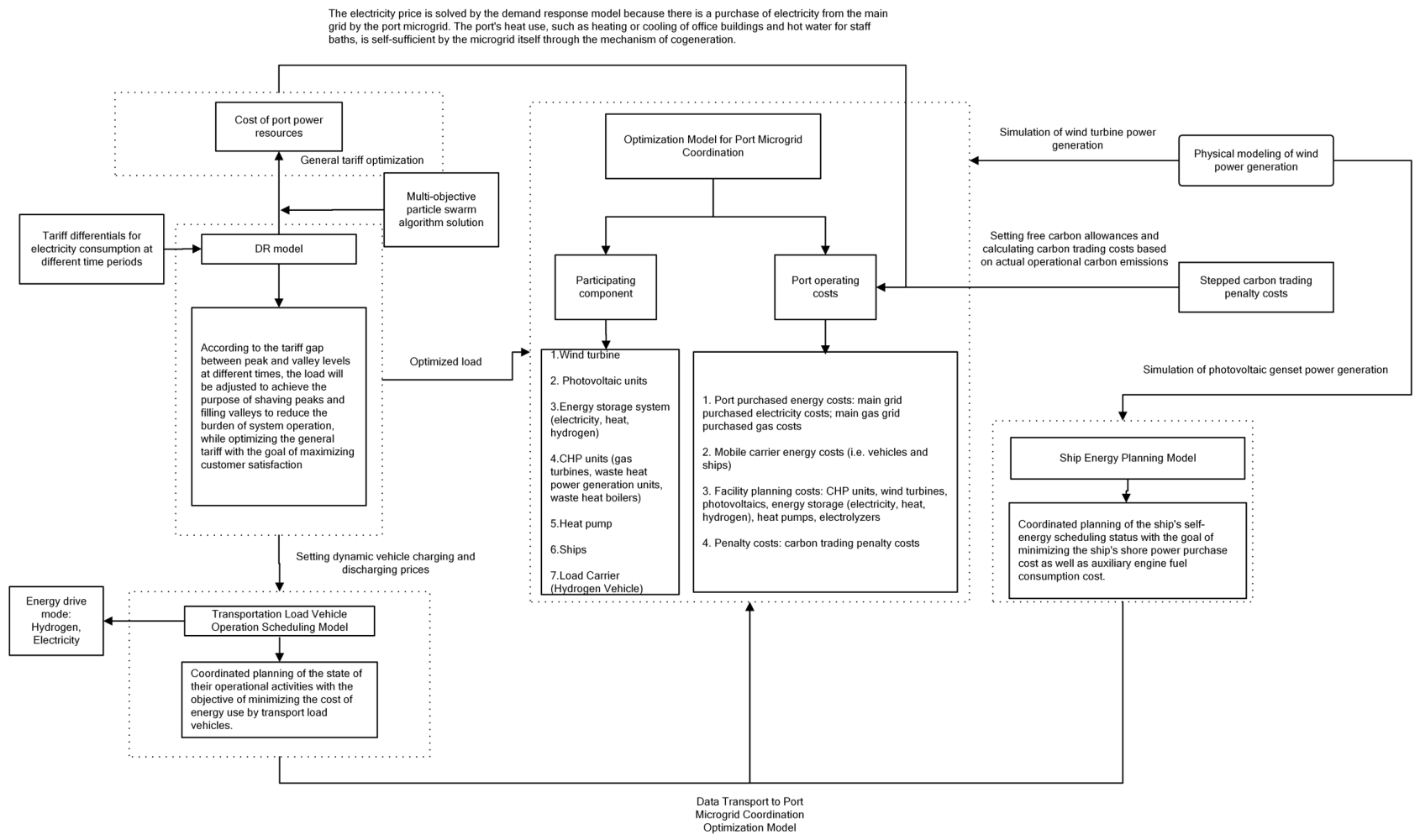
The remainder of the paper is arranged as follows. Section 2 discusses prior work on port vehicle dispatching, ship energy management, and port microgrid operation. Section 3 explains the proposed mechanism and builds the demand response, wind–solar generation, berthed-vessel, heavy-duty-vehicle, and tiered carbon-penalty models. Section 4 presents the cost terms and operating constraints of the coordinated energy management model. Section 5 reports the simulation results. Section 6 summarizes and validates the scenario results, and Section 7 concludes the paper and outlines future research. Figure 1 summarizes the research process, from identifying the low-carbon port scheduling problem to constructing the model and testing demand response and carbon penalties in comparative scenarios.

2. Literature Review

2.1. Port Vehicle Operation Dispatch Management

A port is the transfer point at which maritime transport meets inland distribution, so terminal logistics strongly affect both supply-chain efficiency and energy consumption. Better vehicle organization can reduce waiting time, improve service reliability, and avoid avoidable fuel or electricity use. Vehicle routing, truck assignment, and terminal scheduling have therefore become central topics in port operations research.
One research stream focuses on truck scheduling and the coordination of quay-side and yard-side activities. X. Chen [6] used stochastic operational data from real terminals to design a genetic-programming heuristic for dynamic truck dispatch. X. Chen [7] later extended this line of work through a two-tier genetic-programming hyper-heuristic that accounts for uncertainty in seaside handling and yard operations. B. Xu [8] studied container terminal recovery under large disruptions by coordinating external-truck arrivals and emergency-material priorities, reducing both congestion and operating cost. H. Li [9] proposed a precise-execution-based scheduling method for automated intelligent vehicles, improving terminal efficiency and vehicle energy performance. Y. Chen [10] incorporated capacity and distance constraints into a two-stage model for trailer routing and sequencing under stochastic demand. H.P. Hsu [11] combined yard storage, vessel stowage, and simulation-based optimization to coordinate yard cranes, yard trucks, and quay cranes. L. Zhen [12] developed an improved backtracking search algorithm and implemented a dispatch decision-support system for a Shanghai logistics company. These studies improve vehicle routing, task allocation, and operation sequencing, but their primary concern is logistics efficiency. The energy-supply behavior of low-carbon heavy-duty vehicles and their coupling with port energy systems still receives limited attention.

2.2. Ship Self-Energy Dispatch Management

Emission-control pressure has accelerated the use of renewable and hybrid power systems on ships, making the interface between vessels, shore power, and port energy management more important. Existing work mainly studies hybrid ship power-system scheduling. J. Hou [13] developed adaptive model predictive control for hybrid energy storage, reducing the effect of parameter uncertainty on power allocation and dynamic response. Y. Xu [14] considered multi-energy ship microgrids under continuous roll conditions and integrated AC/DC renewable-energy networks, showing that coordinated energy and voyage scheduling can reduce cost and risk. C.S. Edrington [15] proposed distributed energy management for a four-zone ship power system with storage, with attention to load satisfaction and ramp-rate constraints. K. Hein [16] studied shore-to-ship power and solar-assisted hybrid ferries through a two-stage multi-objective model that balances operating cost and storage degradation. L. Xu [17] addressed non-convex power-management problems with a multi-population particle swarm algorithm using historical and central-particle information. K. Hein [18] further combined data-driven navigation and all-electric ship energy scheduling with NSGA-II, NSGA-III, and LSTM-based photovoltaic forecasting. Z. Wang [19] optimized a ship-side multi-energy system covering electricity, heating, and cooling devices. Z. Li [20] verified the cost and emission benefits of multi-objective coordinated energy and voyage scheduling. S.I. Taheri [21] studied diesel-generator dispatch in maritime power systems, and S. Wen [22] incorporated shore-power prices into joint generation and voyage scheduling for all-electric ships. These studies confirm the value of ship-side energy scheduling, but they usually take the vessel as the main system boundary. The interaction among berthed ships, shore-power demand, port microgrids, and land-side vehicle energy demand remains insufficiently integrated.

2.3. Port Microgrid Energy Management

Ports concentrate distributed generation, conversion equipment, storage devices, shore-power facilities, and terminal loads in a compact operating area. Prior studies show that renewable generation, storage operation, and bidirectional energy exchange can be optimized together to improve cost and emission performance [23,24,25]. A modern port can therefore be treated not only as a logistics node but also as a microgrid with distinctive load rhythms and operational constraints.
A microgrid contains distributed generators, storage resources, and both controllable and uncontrollable loads; demand can be met locally or through electricity purchased from the main grid [26]. Higher renewable penetration also brings more uncertainty because wind and photovoltaic outputs depend on weather forecasts and intermittent resource conditions. Forecast errors may create supply-demand mismatches and threaten service quality. Storage is therefore essential because it absorbs surplus renewable electricity during high-output periods and releases energy when demand is high or renewable output is weak.
Storage has been used for load shifting [27], arbitrage [28], power-quality support [29], cost reduction [30,31], and peak shaving [32]. W. Huang [23] proposed a compressed reconstruction method for port microgrid operating scenarios and built a linearized sizing model for renewable energy and storage. C. Iris [24] formulated a mixed-integer model for port microgrid operation under renewable uncertainty, considering electricity tariffs and bidirectional trading; the results showed the cost-saving potential of storage and renewable utilization. S. Fang [33] embedded flexible logistics loads into an unbalanced multiphase distribution network and thermal network, using iterative convex relaxation for the nonlinear problem. Y. Tao [34] designed a spatiotemporal voyage scheduling strategy to reduce all-electric ship charging pressure on island grids. Z. Ban [35] studied distributed energy management and topology construction with convergence and communication-distance considerations. N.N.A. Bakar [36] used HOMER to size a hybrid microgrid for Aalborg Port using solar, temperature, and wind data. X. Wang [25] proposed day-ahead economic dispatch for an integrated port energy system with hydrogen, reducing both energy and carbon-emission costs. These contributions indicate that port energy management is moving from single-carrier dispatch toward coordinated multi-energy operation with renewable generation, storage, and flexible loads.
Low-carbon port operation has become another active research direction. F. Teng [37] proposed a distributed low-carbon energy management method for port microgrids based on we-energies and verified its economic and emission-reduction effects. Q. Shan [38] incorporated carbon capture and storage into port microgrid management and used a multi-agent consensus algorithm for grid-connected, islanded, and mode-switching operation. J. Song [39] designed a zero-carbon port microgrid with a carbon capture plant and solved the distributed management problem with the alternating direction method of multipliers. These studies show that carbon-oriented constraints are essential for port microgrid operation. More recent work also applies multi-agent reinforcement learning to flexible resource management under uncertain renewable output and dynamic demand. For example, Wu et al. [40] proposed an adaptive virtual-power-plant framework for dynamic multi-energy buildings, but the link with port-specific logistics loads such as berthed ships and heavy-duty vehicles is still limited.
In summary, existing research usually treats port microgrid operation, ship energy scheduling, and vehicle dispatching as separate problems. A unified formulation that simultaneously coordinates berthed ships, land-based heavy-duty vehicles, renewable generation, hydrogen production and storage, demand response, and tiered carbon penalties is still lacking. This gap motivates the present study, which links maritime-side and land-side energy demand within one economic and low-carbon dispatch framework.

3. Model Mechanism Analysis and Related Model Design

3.1. Model Mechanism Analysis

Port production relies on quay cranes, cargo-handling machinery, yard equipment, transport vehicles, and ships at berth. These activities create concentrated energy demand and are also important sources of direct and indirect emissions. Under carbon-peaking and carbon-neutrality targets, ports need to electrify high-consumption links, improve the carrying capacity of distribution networks, and raise the share of locally consumed renewable energy. Renewable resources should support both terminal equipment and berthed ships, while storage and dispatch decisions coordinate supply across the whole port area.
In this transition, renewable-energy utilization is the technical foundation of green port development. Wind and photovoltaic resources can be embedded into the port system through equipment integration and coordinated scheduling, thereby meeting part of the growing energy demand with lower emissions. Demand response adds flexibility on the load side by guiding consumption away from congested or high-price periods, which helps reduce peak-valley pressure and electricity expenses.
A tiered carbon-trading penalty provides an additional economic signal. Once actual emissions exceed the free quota, the marginal cost of further emissions rises by interval, encouraging cleaner energy substitution and more efficient dispatch. Low-carbon operation is therefore shaped by both technical feasibility and explicit emission-cost incentives.
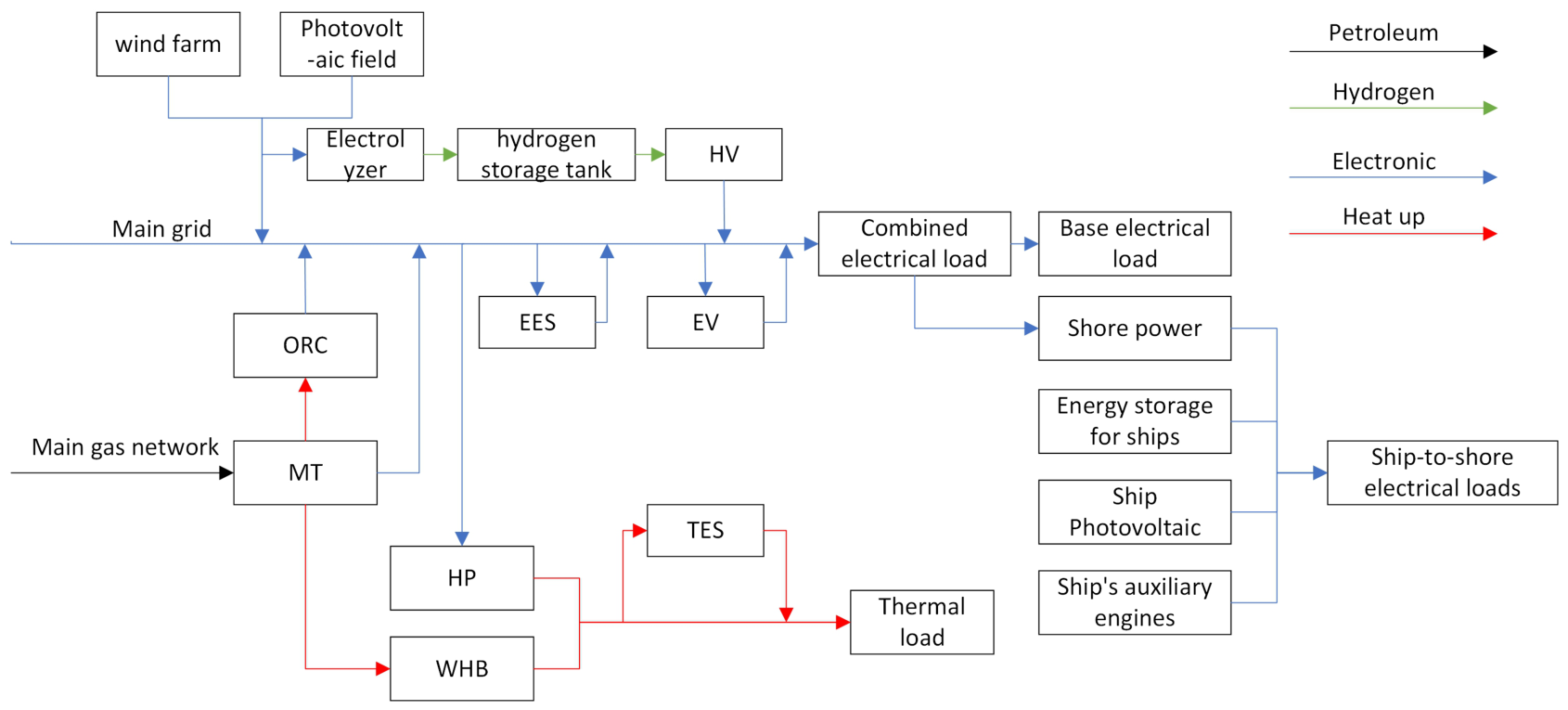
Based on this logic, the paper builds a coordinated port microgrid optimization model that includes ships, handling equipment, vehicles, multi-energy resources, and carbon emissions. The model consists of demand response, wind–solar output, berthed-ship energy scheduling, heavy-duty-vehicle dynamic planning, and tiered carbon-penalty modules, as detailed in Section 3.2. Figure 2 presents the interaction mechanism among renewable generation, flexible demand, berthed-vessel loads, heavy-duty vehicle operation, and carbon-penalty signals.

3.2. Related Models

3.2.1. Demand Response Model

Electricity price spreads can change the timing of flexible consumption and thus provide a demand-side dispatch tool. Zhang [41] used a Logistic function to describe price-based demand response. In this paper, the Logistic framework is applied only to the price-sensitive share of port electricity demand, not to all loads. Flexible participants include adjustable hydrogen production, selected electric-vehicle charging, storage charging, and non-critical auxiliary loads. By contrast, basic cold-ironing demand, safety-related consumption, and essential cargo-handling loads are regarded as inelastic or only weakly responsive.
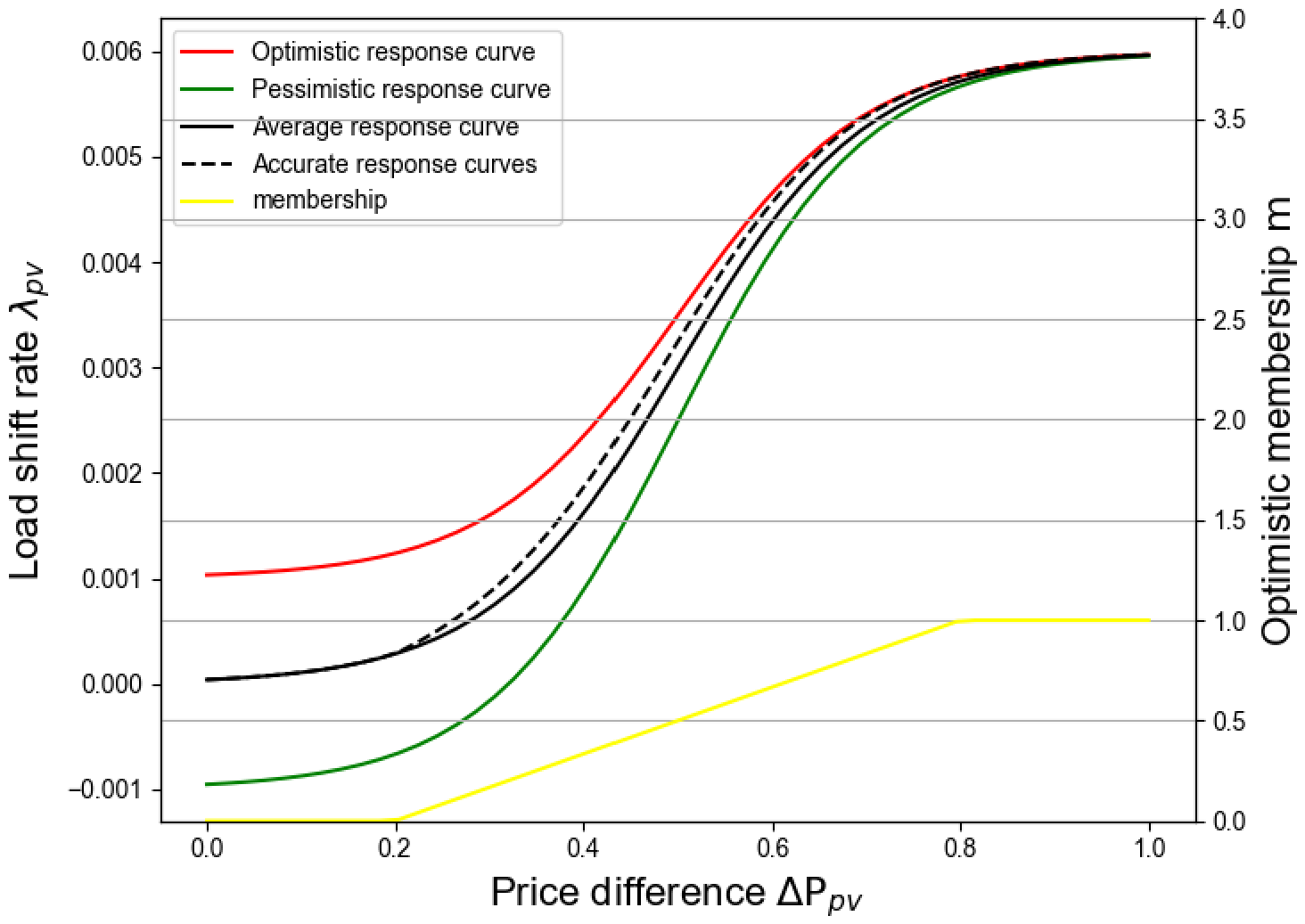
User response to price incentives is uncertain. The realized response is therefore bounded by optimistic and pessimistic curves that represent possible variation in load-shifting behavior. Taking the peak–valley spread as the representative case, a fuzzy Logistic response mechanism is constructed. In this mechanism, Δ P p v denotes the peak–valley price difference, and λ p v denotes the peak–valley transfer rate, measured as shifted peak-valley load divided by the average peak load. The parameters a, b, c, μ , a p v , and b p v control the response intensity, transition point, and interval boundaries of the flexible-load response curve.
The response curve is divided into three zones. In the dead zone, the price spread is too small to produce meaningful adjustment. In the response zone, a larger spread encourages more users to shift demand across periods. In the saturation zone, most flexible demand has already been shifted, so additional price changes produce little extra response. Without time-of-use price differences, load adjustment is more random and less controllable.
The function model of the fuzzy response mechanism based on the Logistic function is shown as
λ p v ( Δ P p v ) = a 1 + e ( Δ P p v c ) / μ + b Δ P p v = P p P v
where a, b, c, and μ are constants of the Logistic function, and P p and P v represent the peak and valley electricity prices, respectively.
Optimistic and pessimistic response curves are fitted to represent the range of possible effects of time-of-use tariffs. The model then introduces behavioral randomness and the membership degree of optimistic response to probabilistically restrict the realized response. Small price changes lead to weak transfer in the dead zone, the transfer rate rises quickly in the response zone, and the response approaches its upper bound in the saturation zone because the remaining flexible demand is limited. The membership-degree formulation is given below:
The specific calculation formula is
λ p v ¯ = ( λ p v o p + λ p v p e ) / 2 , 0 Δ P p v a p v λ p v p e + ( 1 + m ) ( λ p v o p + λ p v p e ) 2 , a p v Δ P p v b p v λ p v o p , b p v Δ P p v
m = Δ P p v a p v b p v a p v , a p v Δ P p v b p v
where a p v represents the transition node from the dead zone to the response zone; b p v represents the transition node from the response zone to the saturation zone; m represents the membership degree of optimistic response; and λ p v o p and λ p v p e represent the peak-to-valley load transfer rates under optimistic and pessimistic responses, respectively.
Figure 3 illustrates how the peak–valley price spread maps into the load transfer rate.
As Figure 3 shows, the load transfer rate is low in the dead zone, rises rapidly once the response zone is entered, and becomes nearly flat when the price spread is large enough to exhaust most flexible response.
Similarly, the displacement rates of the load from peak to flat and from flat to valley are λ p f ¯ and λ f v ¯ , respectively. According to the above analysis, the accurate shift in load is
Δ D t = λ p f ¯ D p ¯ λ p v ¯ D p ¯ , t T p λ p v ¯ D p ¯ λ f v ¯ D f ¯ , t T f λ p v ¯ D v ¯ + λ f v ¯ D f ¯ , t T v
D t = D t 0 + Δ D t
where D p ¯ , D f ¯ , and D v ¯ represent the average loads in the peak, flat, and valley periods without demand response, respectively; T p , T f , and T v are the sets of peak, flat, and valley periods, respectively; Δ D t represents the accurate load shift under demand response; and D t 0 and D t represent the loads before and after demand response, respectively.
min F 1 D R = 1 T t = 1 T ( D t D ¯ ) 2 max F 2 D R = 1 t = 1 T | Δ D t | t = 1 T D t 0 × 1 t = 1 T p t D t t = 1 T p t 0 D t 0 t = 1 T p t 0 D t 0
1 P p P v 3 P f P p P v P f
where T represents the scheduling period, D ¯ represents the average load after demand response, and p t 0 and p t represent the electricity prices before and after demand response for time t, respectively.

3.2.2. Physical Model of Wind and Solar Power Generation Units

For day-ahead scheduling, forecast meteorological variables are converted into wind and photovoltaic output through physical generation models. The photovoltaic output is calculated as follows [42]:
P P V , t = P P V N I t [ 1 + k ( T a c , t T N ) ] I S R T a c , t = T a m , t + 30 I t 1000
where T a c , t is the actual temperature of illumination at time t, T a m , t is the ambient temperature at time t, T N is the rated temperature of illumination, I t and I S R are the illumination radiation intensity at time t and the rated illumination intensity, respectively, P P V , t is the actual electric power output of the photovoltaic unit at time t, P P V N is the rated output power of the photovoltaic unit, and k is the power temperature coefficient.
Wind-turbine output depends on the actual wind speed and the turbine operating region. With a quadratic approximation between cut-in and rated speed, the wind-power expression is [43]:
P W T , t = 0 , V w , t < V i n , t P W T N V w , t 2 V i n , t 2 V n , t 2 V i n , t 2 , V i n , t V w , t V n , t P W T N , V n , t V w , t V o u t , t 0 , V o u t , t V w , t
where P W T , t is the actual electric power of the wind turbine unit at time t, V i n , t is the cut-in wind speed of the wind turbine unit, V o u t , t is the cut-out wind speed of the wind turbine unit, V w , t is the actual wind speed, and P W T N is the installed capacity of the wind turbine unit.

3.2.3. Berth Ship Model

The berth model considers an intelligent port receiving multiple electric ships. While berthed, a ship can draw shore power from the port microgrid for hotel and auxiliary loads, reducing the need for onboard auxiliary-engine generation but increasing port-side electricity demand. Each ship is assumed to have photovoltaic generation, auxiliary generation, and storage. Arrival time, departure time, and power demand are generated through Monte Carlo simulation.
For ship i, shore power and onboard controllable resources are scheduled together. Shore-power purchase is denoted by P i , t C I ; photovoltaic output is denoted by P i , t P V , l s ; auxiliary generator output is denoted by P i , t a e , l s ; and storage charging and discharging powers at time t are denoted by P i , t c h , l s and P i , t d i s , l s . The berth-level balance is:
P i , t C I + P i , t P V , l s + P i , t a e , l s P i , t c h , l s + P i , t d i s , l s = P i , t l s , i N l s , t T
where P i , t l s represents the load demand of ship i at time t during docking, and N l s and T are the sets of berthed ships and docking time slots, respectively.
Ship arrivals and departures are simulated by Monte Carlo sampling. The arrival time of ship i follows the probability density f i d under a wrapped normal-type distribution [44]:
f i d ( t i d ) = 1 2 π σ d exp ( t i d + 24 μ d ) 2 2 σ d 2 , 0 t i d μ d 12 , 1 2 π σ d exp ( t i d μ d ) 2 2 σ d 2 , μ d 12 t i d 24
where t i d is the arrival time for ship i, μ d is the mean arrival time, and σ d is the standard deviation of arrival time.
The departure time of ship i is represented by the probability density f i o :
f i o ( t i o ) = 1 2 π σ o exp ( t i o μ o ) 2 2 σ o 2 , 0 t i o μ o + 12 , 1 2 π σ o exp ( t i o 24 μ o ) 2 2 σ o 2 , μ o + 12 t i o 24
where t i o is the departure time for ship i, μ o is the mean departure time, and σ o is the standard deviation of departure time.
Because ships arrive and leave at different times, CI availability and shore-power demand vary throughout the scheduling horizon. Under the assumption that berths have the same installed CI capacity, the berthing state of each ship is determined by its arrival and departure times. The state equals 0 outside the berthing interval and 1 during berthing:
B i , t = 0 , t [ 1 , t i d ] 1 , t [ t i d , t i o ] 0 , t [ t i o , T ] , i N l s
Constrained by berth planning and facility transmission capabilities, the CI power P i , t C I is
B i , t P C I , min P i , t C I B i , t P C I , max
where B i , t is a binary variable indicating whether ship i is in a berthed state, and P C I , min and P C I , max are respectively the minimum and maximum power that can be drawn from the port.
For ship-side storage, charging and discharging powers in each time slot are bounded by their maximum levels:
0 P i , t c h , l s S i , t c h , l s P i c h , l s , max , i N l s , t T
0 P i , t d i s , l s S i , t d i s , l s P i d i s , l s , max , i N l s , t T
where S i , t c h , l s and S i , t d i s , l s are the charging and discharging state variables of the storage system. To ensure mutual exclusivity of the charging and discharging states, the implementation of these state variables is
0 S i , t d i s , l s + S i , t c h , l s 1 , i N l s , t T
The energy level of ship i evolves according to its charging and discharging decisions:
E i , t + 1 s , l s = E i , t s , l s + P i , t c h , l s μ i s , l s P i , t d i s , l s μ i s , l s , i N l s , t T
where μ i s , l s is the charging and discharging efficiency coefficient of ship i’s energy storage system. The energy level must be maintained within allowable limits:
E i s , l s , min E i , t s , l s E i s , l s , max , i N l s , t T
0 P i , t P V , l s P i P V , max
where E i s , l s , min and E i s , l s , max represent the minimum and maximum energy levels, respectively, and P i P V , max is the maximum power generation capacity of the photovoltaic system. The power generation of AG, denoted by P i , t a e , l s , is constrained by its generation capacity P i , t a e , l s , max and carbon emission constraints:
0 P i , t a e , l s P i , t a e , l s , max , i N l s , t T
S i , t a e , l s a i e m , l s P i , t a e , l s E m i max , i N l s , t T
where S i , t a e , l s represents the operational state of the auxiliary engine on ship i, being 1 if on and otherwise 0, a i e m , l s is the carbon emission coefficient for AG, and E m i max is the maximum emission limit.

3.2.4. Dynamic Programming Model for Port Heavy-Duty Transport Vehicles

Heavy-duty trucks move loaded and empty containers among quays, yards, and nearby warehouses. To maintain terminal service while reducing vehicle energy cost, this section develops a dynamic scheduling model for hydrogen and electric heavy-duty vehicles. Hydrogen vehicles are assigned among transport, refueling, and idle states. Electric vehicles are assigned among transport, charging, discharging, and idle states. The hydrogen-vehicle operating state is expressed as:
φ T a = t = 1 T j = 1 N H V x j , t H V , a , a = 1
where φ T a represents the number of containers transported back and forth by the hydrogen heavy-duty transport vehicles within one day, and x j , t H V , a is a 0–1 variable representing the operational status of the jth hydrogen heavy-duty transport vehicle at time t, categorized into three states: transportation, hydrogen refueling, and idle. When in state a, x j , t H V , a is 1; otherwise, it is 0. The model constraints are noted below:
φ T a T a
where T a represents the daily container throughput of the port, ensuring that the transport load of heavy-duty vehicles meets the port’s throughput needs.
a = 1 3 x j , t H V , a = 1 , j , t
This constraint ensures that each vehicle performs at most one task in a time slot. Hydrogen heavy-duty vehicles are initially assumed to remain idle from 1:00 AM to 4:00 AM, after which dispatching begins with a hydrogen-tank level of 100 % .
H L j , t H V = H L j , t 1 H V x j , t H V , 1 ω j , t H V H j , H V c a p + x j , t H V , 2 R j , t H V , r e f H j , H V c a p H L j , min H V H L j , t H V H L j , max H V , j , t
where H L j , t H V is the hydrogen-tank level of the jth hydrogen heavy-duty transport vehicle; H j , H V c a p is the maximum hydrogen capacity of the vehicle; ω j , t H V is the hydrogen consumption of the vehicle during transportation at time t; R j , t H V , r e f represents the hydrogen refueling amount at time t; and H L j , min H V and H L j , max H V are respectively the minimum and maximum allowable hydrogen-tank levels.
Electric heavy-duty vehicles are modeled through battery SOC dynamics and may participate in both charging and vehicle-to-grid discharging. They are therefore not only mobile loads but also temporary storage resources. Charging and discharging are mutually exclusive. This study assumes that electric trucks respond to price-guided charging and discharging signals: charging prices rise during high-load periods to discourage additional demand, while discharging prices compensate vehicles that support the port grid. The optimized charging and discharging prices are:
P t E V C p r i c e = P t , p E V C p r i c e 1 + D t D ¯ D ¯ , t T p P t , f E V C p r i c e 1 + D t D ¯ D ¯ , t T f P t , v E V C p r i c e 1 + D t D ¯ D ¯ , t T v
P t E V D p r i c e = P t , p E V D p r i c e 1 + D t D ¯ D ¯ , t T p P t , f E V D p r i c e 1 + D t D ¯ D ¯ , t T f P t , v E V D p r i c e 1 + D t D ¯ D ¯ , t T v
where P t E V C p r i c e and P t E V D p r i c e are the optimal charging and discharging prices for electric vehicles at time t; P t , p E V C p r i c e , P t , f E V C p r i c e , and P t , v E V C p r i c e are the optimal electric vehicle charging prices at peak, flat, and valley periods; and P t , p E V D p r i c e , P t , f E V D p r i c e , and P t , v E V D p r i c e are the optimized electric vehicle discharging prices at peak, flat, and valley periods.

3.2.5. Tiered Carbon Trading Penalty Model

A tiered carbon-trading mechanism turns excess emissions into dispatch costs through tradable allowances and interval-based penalties [42]. Because China’s carbon market is still evolving, free allowances are often assigned by regulators. Enterprises emitting less than their allowance may sell surplus quotas, whereas enterprises exceeding the allowance must buy additional quotas or bear penalty costs. This paper uses the baseline method to determine free allowances, compares actual emissions with the allowance benchmark, and charges excess emissions through a tiered price. The five-tier structure is a scenario-based modeling assumption that captures increasing marginal emission costs; it is not intended to reproduce a specific port regulation. When excess emissions move into higher intervals, the marginal penalty rises and strengthens the incentive for low-carbon operation.
E I E S , c = E I E S , a E I E S
where E I E S is the total free carbon emission quota of the system, E I E S , a is the actual carbon emissions of the system, and E I E S , c is the difference between actual carbon emissions and free carbon emission quota.
E I E S = E e , b u y + E g , c h p + E a e , s h i p s
E e , b u y = σ b u y t = 1 T P e , b u y ( t ) E g , c h p = σ c h p t = 1 T P g , c h p ( t ) E a e , s h i p s = σ a e t = 1 T P a e , s h i p s ( t )
where E e , b u y , E g , c h p , and E a e , s h i p s respectively represent the free carbon emission quotas for buying electricity from the main grid, purchasing gas from the main gas network by CHP units, and fuel consumption of the auxiliary engines of ships, where σ b u y , σ c h p , and σ a e are the free carbon emission quota coefficients; and P e , b u y , P g , c h p , and P a e , s h i p s respectively represent the power for the port to purchase electricity from the grid, the volume of gas purchased by the CHP units from the main gas network per unit time, and the power supply of the auxiliary engines of ships at the port per unit time.
E I E S , a = E e , b u y , a + E g , c h p , a + E a e , s h i p s , a
E e , b u y , a = σ b u y , a t = 1 T P e , b u y ( t ) E g , c h p , a = σ c h p , a t = 1 T P g , c h p ( t ) E a e , s h i p s , a = σ a e , a t = 1 T P a e , s h i p s ( t )
where E e , b u y , a , E g , c h p , a , and E a e , s h i p s , a respectively represent the actual carbon emissions for components such as thermal power plants, CHP units, photovoltaic units, wind power units, and so on purchased from the main grid, where σ b u y , a , σ c h p , a , and σ a e , a are the actual emission coefficients.
C c o 2 = λ E I E S , c , E I E S , c d λ ( 1 + α ) ( E I E S , c d ) + λ d , d E I E S , c 2 d λ ( 1 + 2 α ) ( E I E S , c 2 d ) + λ ( 2 + α ) d , 2 d E I E S , c 3 d λ ( 1 + 3 α ) ( E I E S , c 3 d ) + λ ( 3 + 3 α ) d , 3 d E I E S , c 4 d λ ( 1 + 4 α ) ( E I E S , c 4 d ) + λ ( 4 + 6 α ) d , 4 d E I E S , c 5 d λ ( 1 + 5 α ) ( E I E S , c 5 d ) + λ ( 5 + 10 α ) d , 5 d E I E S , c
where C c o 2 represents the cost of tiered carbon trading, λ is the base price, α is the price growth rate, and d is the carbon emission growth interval.

4. Port Microgrid Coordinated Optimization Model

This section formulates a coordinated optimization model for a port microgrid under practical operating conditions, with particular attention to freight vehicles and ships at berth. The model includes handling equipment, transport vehicles, berthed vessels, and other energy-consuming users from a port-wide scheduling perspective. Without coordinated dispatch, energy allocation can become inefficient, operating cost can rise, and terminal service reliability can deteriorate. The optimization model is therefore designed to balance logistics demand, energy supply, and economic performance.
For low-carbon development, the port power network must do more than transmit and distribute electricity. It also needs renewable-energy infrastructure such as photovoltaic stations and wind farms. These resources provide cleaner supply but introduce intermittency. To maintain reliability, the port may still purchase electricity, natural gas, and thermal energy from external networks. The model therefore coordinates renewable output, conventional purchases, conversion devices, and storage resources in one dispatch framework.
Demand-side management is introduced through the demand response module. By guiding flexible loads to adjust consumption timing, the module supports supply-demand balance, improves operating efficiency, and reduces electricity cost. By jointly considering demand, renewable utilization, and network stability, the model provides a basis for efficient low-carbon port microgrid operation.
The objective function minimizes total operating cost. The cost components include energy purchase, carbon penalty, mobile-equipment energy scheduling, and port equipment usage, which together reflect the operating requirements of a modern port microgrid.

4.1. Total Port Operation Cost Composition

F p o r t = F b u y P o r t + F c a r b o n + F v e h i c a l + F u s e
where F u s e represents equipment-related capital and operating expenditure. In the scenario comparison, this term is reported separately so that the contribution of each operating activity can be observed.

4.1.1. Purchasing Costs

F b u y P o r t = F b u y P o r t , e + F b u y P o r t , g a s
where F b u y P o r t is the total cost of energy purchased by the port, and F b u y P o r t , e and F b u y P o r t , g a s are the cost of electricity purchased by the port from the main grid and the cost of gas purchased from the main gas grid, respectively.
(1)
Cost of Purchasing Electricity from the Main Power Grid
F b u y P o r t , e = C b u y , e t = 1 T P t g r i d
where C b u y , e is the unit cost of purchasing electricity for the port microgrid, and P t g r i d is the amount of electricity purchased from the main power grid during period t.
(2)
Cost of Purchasing Gas from the Main Gas Network
F b u y P o r t , g a s = C b u y , g a s t = 1 T j = 1 J P t g a s
P t g a s = P t C H P , i n H g a s
where C b u y , g a s is the unit cost of purchasing gas for the port microgrid, P t g a s is the amount of gas purchased from the gas network by CHP units during period t, H g a s is the calorific value of natural gas, and P t C H P , i n is the input power of the CHP units during period t.

4.1.2. Carbon Penalty Cost

Because renewable generation and low-carbon heavy-duty vehicles are included, the remaining carbon penalty mainly comes from grid electricity purchases, gas consumed by CHP units, and auxiliary-engine operation by ships during berthing. The penalty rule is defined in Section 3.2. Let F C O 2 denote this carbon-related cost:
F C O 2 = C C O 2

4.1.3. Mobility Vehicle Energy Scheduling Cost

F v e h i c a l = F h v + F e v + F s h i p
where F v e h i c a l is the daily energy-scheduling cost of mobile resources in the port. The terms F h v and F e v refer to hydrogen and electric heavy-duty trucks, respectively, while F s h i p captures ship energy cost during port stays, including shore-power purchases and auxiliary-engine fuel use.
(1)
Energy Scheduling Cost for Hydrogen Heavy Transport Vehicles
F h v = t = 1 T j = 1 N H V P t H V C p r i c e x j , t H V , 2 P j , t H V , c h
where N H V represents the number of hydrogen fuel cell heavy-duty trucks at the port, P t H V C p r i c e represents the unit hydrogen refueling cost of the hydrogen fuel cell heavy-duty trucks, and x j , t H V , 2 is a binary variable representing the hydrogen refueling status of the heavy-duty truck.
(2)
Electric Heavy-Duty Truck Energy Scheduling Costs
F e v = t = 1 T j = 1 N E V P t E V C p r i c e x j , t E V , 2 P j , t E V , c h t = 1 T j = 1 N E V P t E V D p r i c e x j , t E V , 3 P j , t E V , d i s
where N E V represents the number of electric heavy-duty trucks at the port; P t E V C p r i c e and P t E V D p r i c e represent the unit charging cost and the unit discharging cost of the electric heavy-duty trucks, respectively; and x j , t E V , 2 and x j , t E V , 3 are binary variables representing the charging and discharging states of the heavy-duty truck, respectively.
(3)
Ship Energy Scheduling Costs
F s h i p = F C I + F a g
F C I = t = 1 T i = 1 N s h i p P i , t C I C I t p r i c e F a g = t = 1 T i = 1 N s h i p P i , t a g a g t p r i c e
where F C I and F a g represent the electricity purchasing cost of the ship and the auxiliary engine fuel consumption cost, respectively; P i , t C I and P i , t a g represent the shore power electricity power and auxiliary engine output of the ith ship at moment t, respectively; and C I t p r i c e and a g t p r i c e represent the unit cost of the purchased electricity and the unit cost of consumed fuel by the auxiliary engine at moment t, respectively.

4.1.4. Port Equipment Usage Costs

The intra-day scheduling model includes gas turbines, organic Rankine cycle waste-heat units, waste heat boilers, photovoltaic stations, wind farms, electrolyzers, and electric, thermal, and hydrogen storage systems. The equipment usage cost is:
F u s e = t = 1 T [ C M T P M T , t + C O R C P O R C , t + C W H B P W H B , t + C W T P W T , t + C P V P P V , t + C H P P H P , t + C E L E P E L E , t + C E S S , e ( P E S S , e , c h , t + P E S S , e , d i s , t ) + C E S S , h ( P E S S , h , c h , t + P E S S , h , d i s , t ) + C E S S , t ( P E S S , t , c h , t + P E S S , t , d i s , t ) ]
where C M T , C O R C , C W H B , C W T , C P V , C H P , C E L E , C E S S , e , C E S S , h , and C E S S , t are the unit usage costs of gas turbines, waste heat power generation units, waste heat boilers, wind farms, photovoltaic power stations, heat pumps, electrolytic cells, and energy storage systems (electric, hydrogen, thermal), respectively. P M T , t , P O R C , t , P W H B , t , P W T , t , P P V , t , P H P , t , and P E L E , t are the operating power consumption of gas turbines, waste heat power generation units, waste heat boilers, wind farms, photovoltaic power stations, heat pumps, and electrolytic cells at moment t, respectively. P E S S , e , c h , t , P E S S , h , c h , t , and P E S S , t , c h , t are the charging powers of the electric, hydrogen, and thermal energy storage devices at moment t; and P E S S , e , d i s , t , P E S S , h , d i s , t , and P E S S , t , d i s , t are the discharging powers of the electric, hydrogen, and thermal energy storage devices at moment t, respectively.

4.2. Constraints

4.2.1. Storage System Constraints

Three storage forms are considered. Hydrogen storage receives hydrogen produced from surplus electricity through electrolysis and releases it when vehicle or system demand requires it. Electrical storage charges during surplus generation and discharges during high-load or low-renewable periods. Thermal storage buffers heat from heating and conversion devices.
The hydrogen storage constraints are [45]:
V t + 1 E S , h = V t E S , h + u t c h , h P t c h , h u t d c h , h P t d c h , h V E S , h , min V t E S , h V E S , h , max 0 P t c h , h P c h , h , max 0 P t d c h , h P d c h , h , max u t c h , h + u t d c h , h 1
where u t c h , h and u t d c h , h correspond to the hydrogen storage’s charging and discharging state during period t, with the constraint being less than or equal to 1, representing charging, discharging, and a non-charging state. P t c h , h and P t d c h , h signify the hydrogen storage’s charge and discharge capacity for period t, with P c h , h , max and P d c h , h , max as the upper limits. V t E S , h and V t + 1 E S , h denote the hydrogen levels at times t and t + 1 , respectively; and V E S , h , min and V E S , h , max depict the minimum and maximum hydrogen storage capacities.
The electrical storage constraints are [45]:
E t + 1 E S , e = E t E S , e + u t c h , e P t c h , e η c h , e u t d c h , e P t d c h , e η d c h , e E E S , e , min E t E S , e E E S , e , max 0 P t c h , e P c h , e , max 0 P t d c h , e P d c h , e , max u t c h , e + u t d c h , e 1
where u t c h , e and u t d c h , e indicate the charging and discharging states of electrical storage at time t. P t c h , e and P t d c h , e are the corresponding charging and discharging powers. η c h , e and η d c h , e denote the charging and discharging efficiencies. E E S , e , max and E E S , e , min are the upper and lower electrical storage capacities. Because thermal storage follows the same operating logic, its constraints are omitted to avoid repetition.

4.2.2. Energy Supply Device Constraints

Energy supply devices are organized into electrical, thermal, and hydrogen subsystems. The CHP subsystem contains micro-turbines, ORC low-temperature waste-heat generators, and WHB units. Micro-turbines mainly generate electricity, ORC units recover waste heat for additional power output, and WHB units provide heat. Photovoltaic arrays and wind turbines supply renewable electricity, heat pumps provide thermal energy, and electrolyzers convert surplus renewable electricity into hydrogen for storage and vehicle refueling.
(1)
Electrical Supply Device Constraints
0 P t W T P t W T , max 0 P t P V P t P V , max 0 P t M T , e P t M T , e , max 0 P t O R C P t O R C , max n M T , min P t M T , e P t 1 M T , e P t 1 M T , e n M T , max P t O R C = P t M T , h β r O R C P t M T , h = P t C H P , i n h M T P t M T , e = P t C H P , i n e M T
where P t W T , P t P V , P t M T , e , and P t O R C are the active power output of wind turbines, photovoltaic units, micro-turbines, and ORC devices at time period t, respectively; P t M T , h is the thermal power generated by micro-turbines at time period t; P t W T , max , P t P V , max , P t M T , e , max , and P t O R C , max are the maximum active power outputs of WT, PV, MT, and ORC at time period t, respectively; β is the proportion of waste heat allocated by MT units to ORC units; r O R C is the thermal-to-electric efficiency of the ORC unit; e M T is the gas-to-electric efficiency of the MT unit; h M T is the ratio of the thermal power that can be utilized by other equipment after the MT unit converts gas to electricity to the input power of the CHP unit; and n M T , min and n M T , max are the minimum and maximum ramp rates of the gas turbine, respectively.
(2)
Heating Device Constraints
0 P t H P P t H P , max 0 P t W H B P t W H B , max P t W H B = P t M T , h ( 1 β ) r W H B
where P t H P and P t W H B are the thermal outputs of the heat pump and waste heat boiler at time t; P t H P , max and P t W H B , max are their maximum thermal outputs; and r W H B is the WHB waste-heat conversion ratio.
(3)
Hydrogen Energy Device Constraints
An alkaline electrolyzer produces hydrogen using electricity from wind and photovoltaic generation. Stable hydrogen production, storage, and vehicle supply are maintained through the following constraints:
S e l e , t = η e l e τ 1 P e l e , t P t c h , h = S e l e , t P t d i s , h = P t H V , r e f
where S e l e , t is the amount of hydrogen produced by the electrolyzer, η e l e is the operational efficiency of the electrolyzer, τ 1 is the amount of hydrogen produced per kWh of electrical energy, and P e l e , t is the power consumption of the electrolyzer.

4.2.3. Energy Balance Constraints

(1)
Electrical Load Balance Constraint
P t P o r t , e + P t S h i p , e + P t E V , c h + P t H P + P t e l e P t g r i d P t M T , e P t O R C P t P V P t W T P t d c h , e + P t c h , e P t E V , d i s = 0
where P t E V , c h and P t E V , d i s are the aggregate charging and discharging powers of electric heavy-duty vehicles at time t. EV charging is therefore modeled as an electrical load, while EV discharging is modeled as a flexible supply contribution.
(2)
Thermal Load Balance Constraint
P t l o a d , h = P t W H B + P t H P P t c h , h + P t d c h , h
where P t l o a d , h is the system’s thermal load at time t.

5. Simulation Analysis and Discussion

5.1. Model Parameters

The case-study parameters are drawn from related literature and scenario-based simulation assumptions. Settings for CHP units, electric-vehicle charging and discharging, demand response, and the carbon-trading penalty mechanism are adapted from the coordinated optimization framework in Ma et al. [42]. Parameters for port equipment, vessels, hydrogen trucks, and electric trucks are then adjusted to match the scale and modeling requirements of the proposed integrated port energy system. The case study should therefore be interpreted as a controlled simulation of typical port energy-management conditions rather than a direct measurement dataset from a specific terminal.
Table 1, Table 2, Table 3 and Table 4 list the parameters of port equipment, vessels, hydrogen trucks, and electric trucks. The ADN coordinated optimization model was solved in MATLAB Release 2022a (R2022a) on a 64-bit computer equipped with a 12th-generation Intel Core i9-12900K CPU at 3.20 GHz and 16 GB RAM.

5.2. Solving the DR Model Using Multi-Objective Particle Swarm Optimization

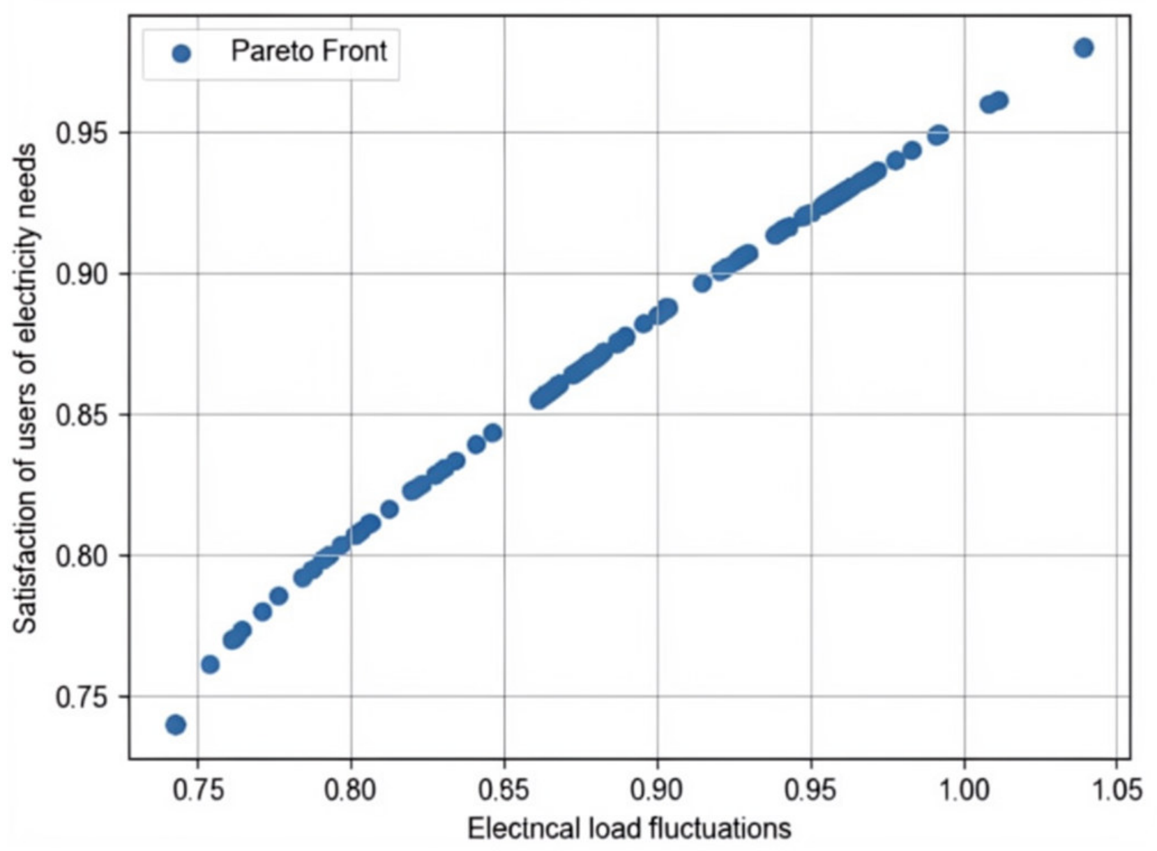
The demand response model is built from the perspective of consumer behavior. It captures how peak, flat, and valley electricity prices affect flexible load demand, with two objectives: maximizing user satisfaction and minimizing the load fluctuation rate. Multi-objective particle swarm optimization is used to solve the model, and the results are shown in Figure 4 and Figure 5.
Figure 4 presents the Pareto frontier between the two objectives. The frontier shows that lower load fluctuation and higher user satisfaction cannot always be improved simultaneously. Because multi-objective particle swarm optimization searches through a population of particles, it can approximate a set of non-dominated solutions and provide several feasible price-response strategies for decision makers.
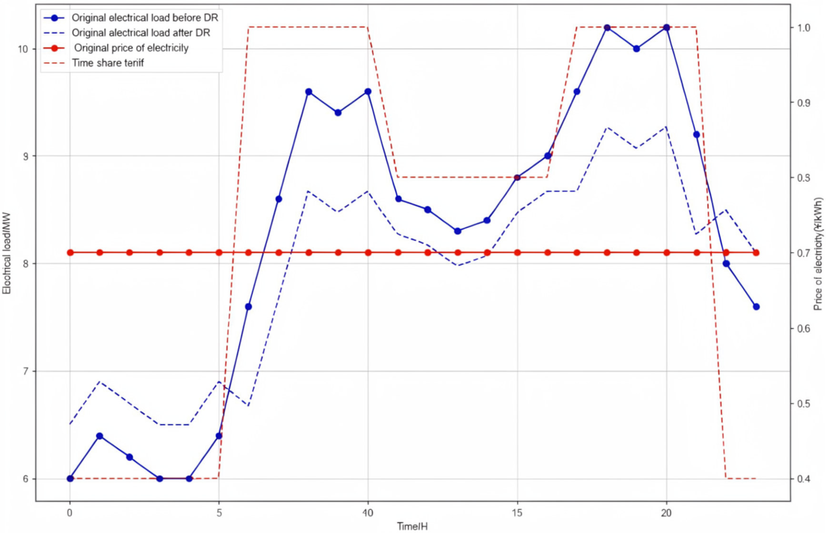
Figure 5 compares the price and load profiles before and after demand response. After the optimized time-of-use price differentials are applied, part of the load moves from peak periods to off-peak periods. Table 5 shows that user satisfaction decreases only modestly, while the load fluctuation rate falls by 56.93 % . This result reflects the assumed participation of flexible loads and should not be interpreted as evidence that all port electricity demand is fully price-elastic.
Thus, the optimized demand response strategy smooths system load while keeping user satisfaction within an acceptable range.
Overall, demand response improves system efficiency by using price signals to shift flexible consumption. Moving load away from peak periods can lower operating pressure, reduce cost, and create more room for renewable-energy utilization.

5.3. Dynamic Programming Model Solution for Heavy Transport Vehicles

This subsection analyzes heavy-duty port vehicles under hydrogen and electric drive modes. The purpose is to show how vehicle operation affects port energy scheduling and how low-carbon fleets can support green port construction.

5.3.1. Impact of Optimizing Charging and Discharging Price Strategies on the Cost of Electric Vehicle Usage

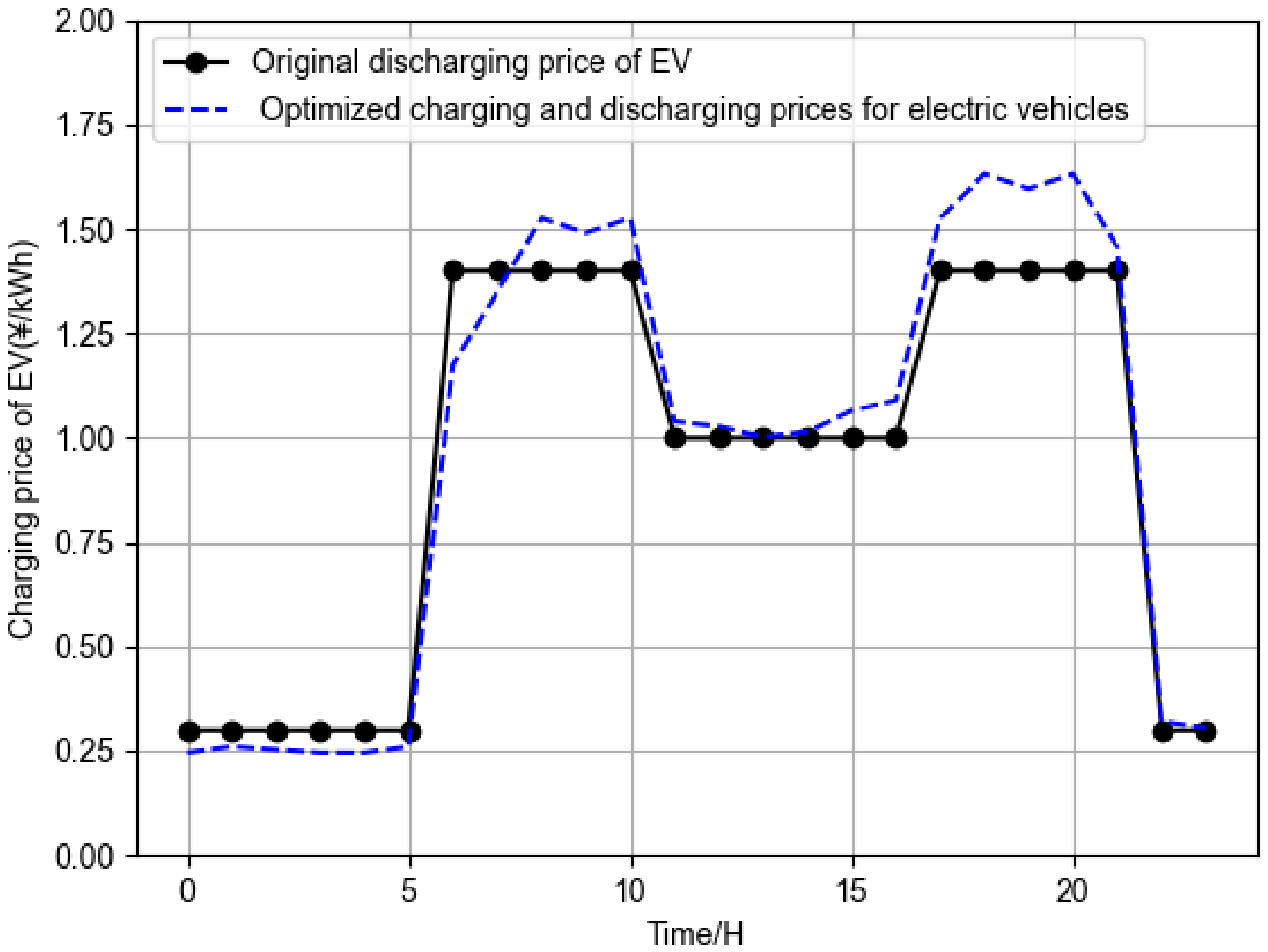
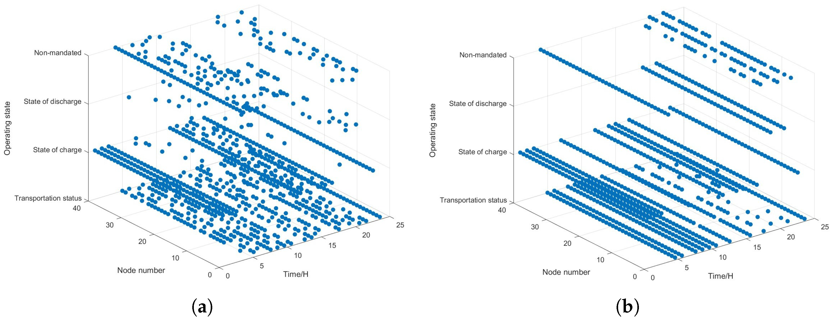
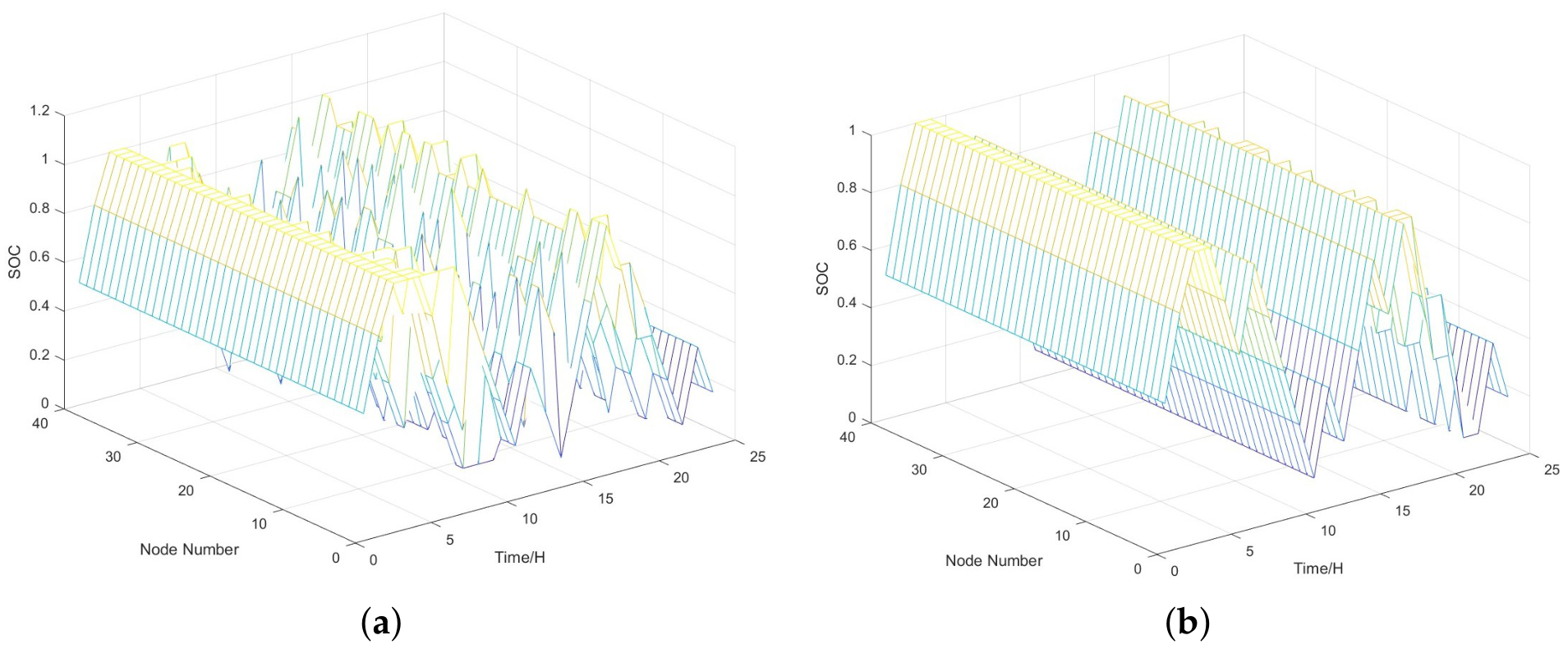
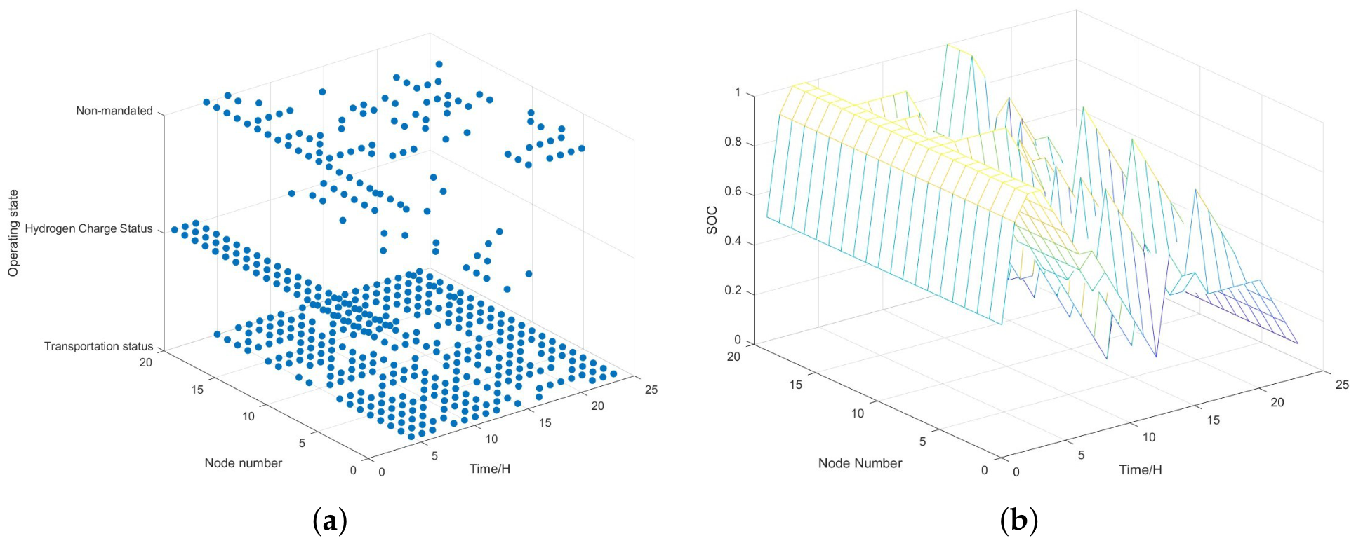
Electric heavy-duty vehicles act as both cargo-transport equipment and mobile storage resources. The initial case sets charging and discharging prices equal. Figure 6 compares this original profile with the optimized dynamic charging and discharging prices, while Figure 7 and Figure 8 report the resulting vehicle states and SOC trajectories. During high-load periods, uncontrolled charging can aggravate grid pressure. The optimized strategy raises charging prices to suppress additional demand and increases discharging compensation to encourage vehicle-to-grid support. Figure 7 shows that more vehicles discharge during high-load intervals and more vehicles charge during low-load intervals. Figure 8 indicates that the resulting schedules remain within SOC limits. Table 6 shows that discharge revenue grows more than charging expenditure, reducing the total vehicle energy-use cost from 22,800 RMB to 18,812.44 RMB.

5.3.2. Interaction Between Ports and Hydrogen Vehicles

Hydrogen-fueled vehicles are a practical low-carbon option for port transport because fuel cells convert hydrogen into electricity for propulsion. Given the conversion efficiency and operating characteristics considered in this study, hydrogen-vehicle energy cost is measured as refueling cost, and no discharge revenue is included.
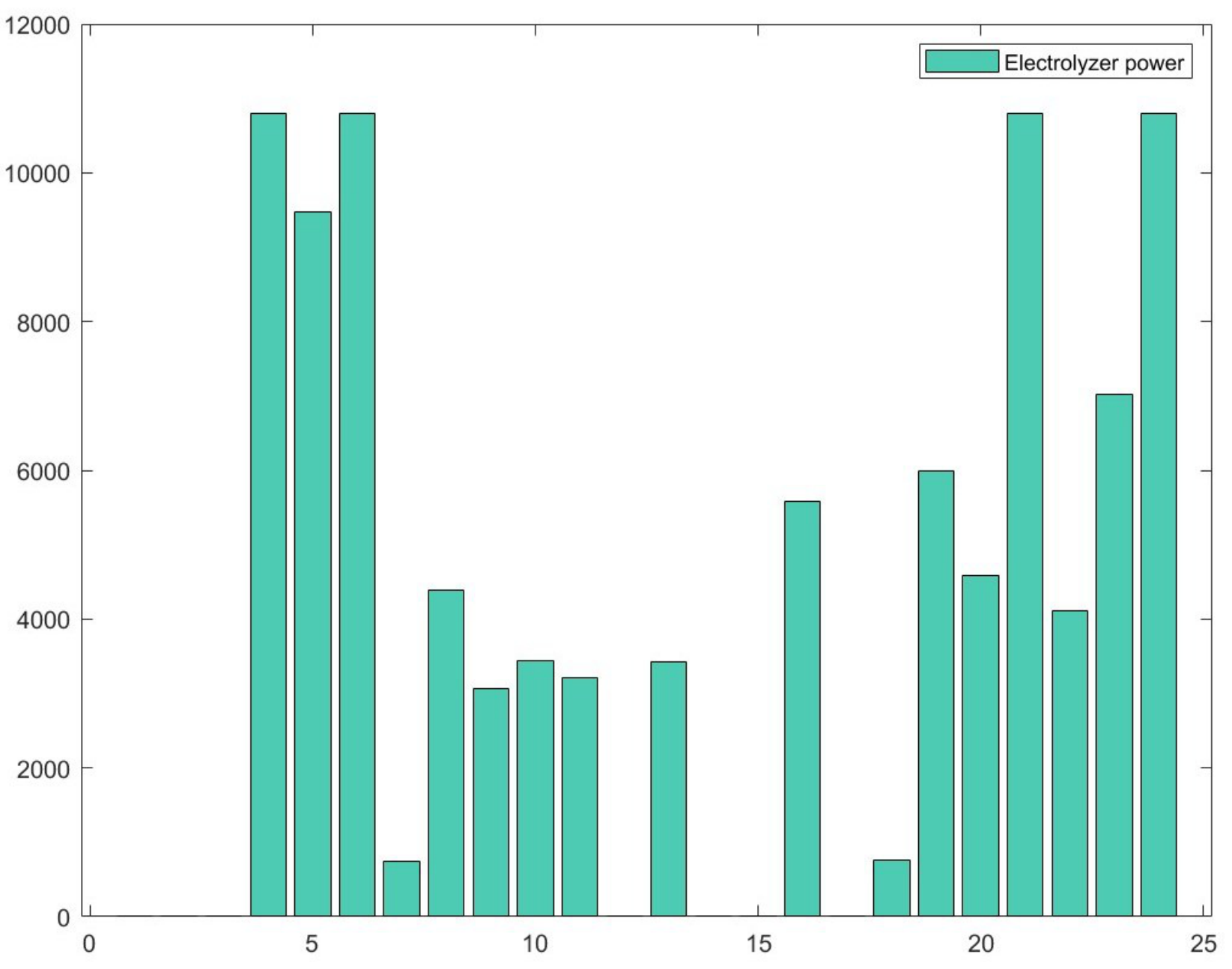
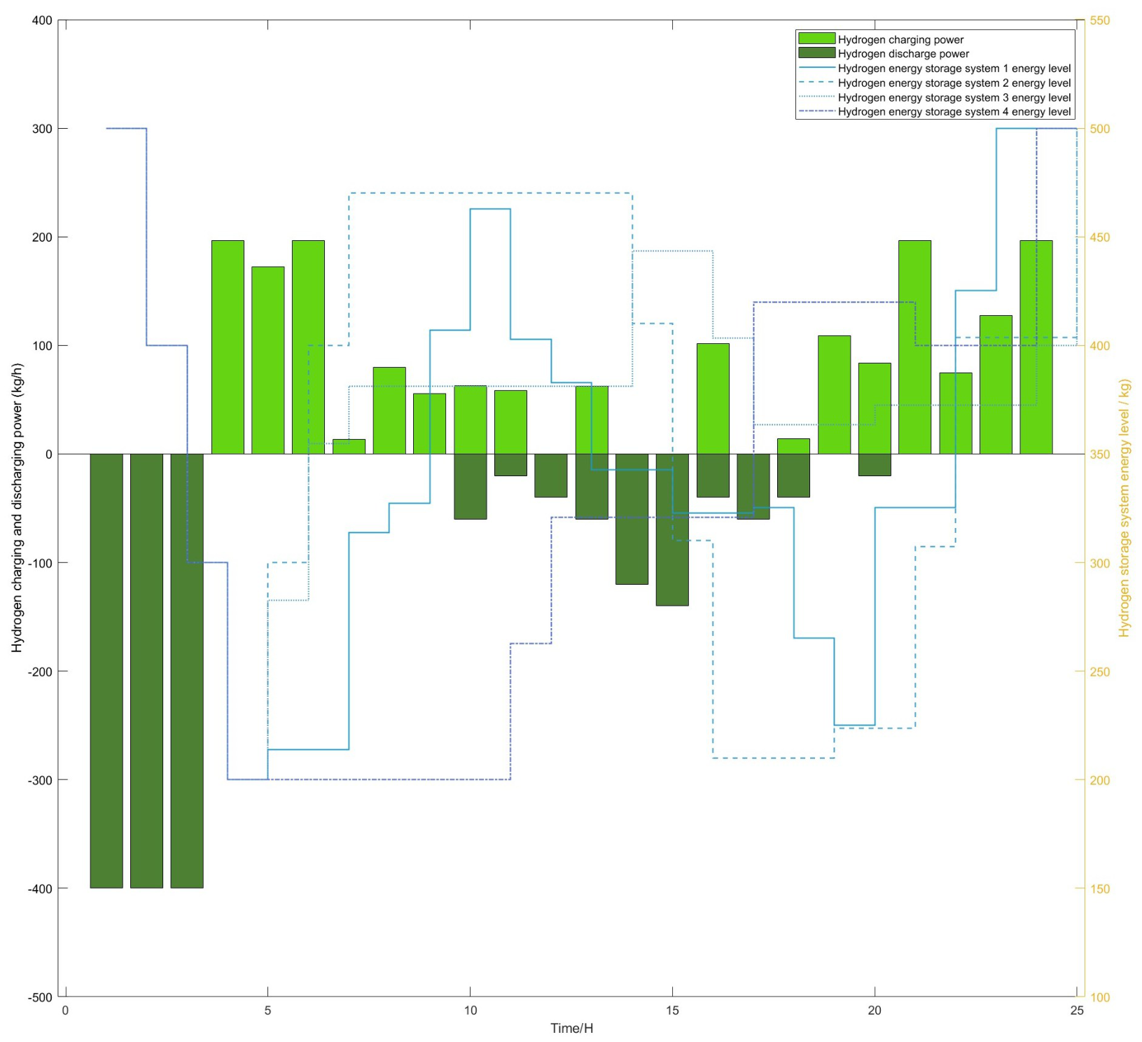
The proposed system uses wind and photovoltaic electricity for electrolysis, stores the produced hydrogen, and supplies it to vehicles according to demand. Figure 9 shows electrolyzer power consumption, Figure 10 shows the 24-h hydrogen storage state, and Figure 11 reports vehicle operating states and tank levels. Because hydrogen vehicles mainly operate from 4:00 AM to 24:00, daytime refueling demand is relatively high, and the electrolyzer operates more intensively to maintain storage. During nighttime rest periods, hydrogen demand falls and electrolyzer load decreases. The results indicate that the production–storage–use chain can satisfy daily transport demand while keeping storage operation feasible.

5.4. Comprehensive Energy Planning Model for Vessels at Berths

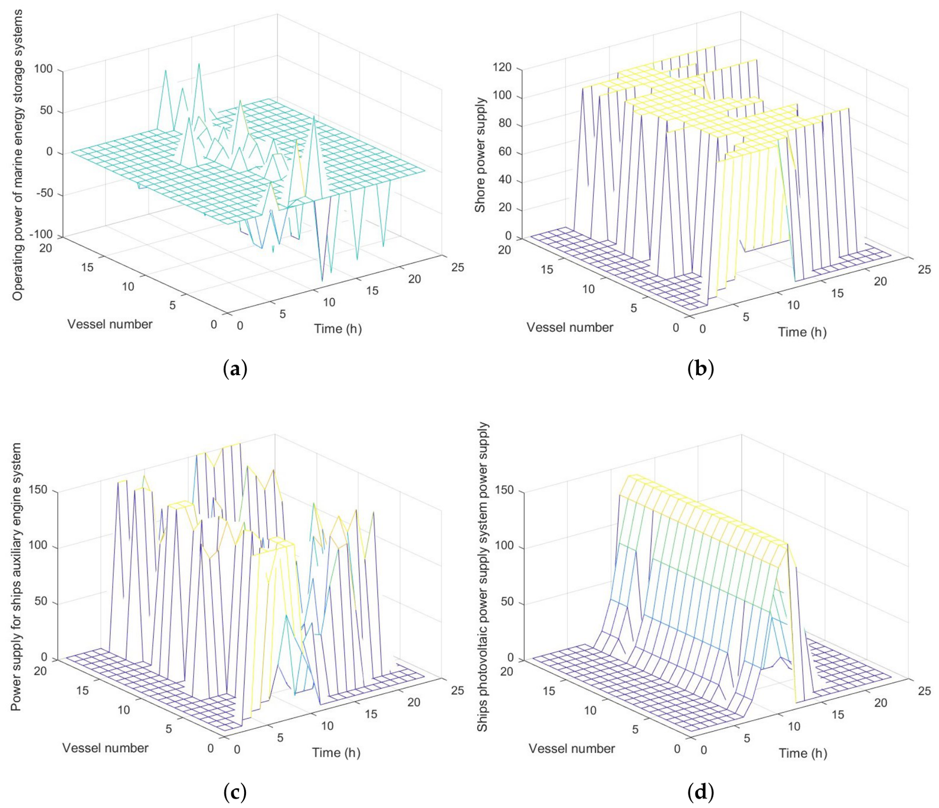
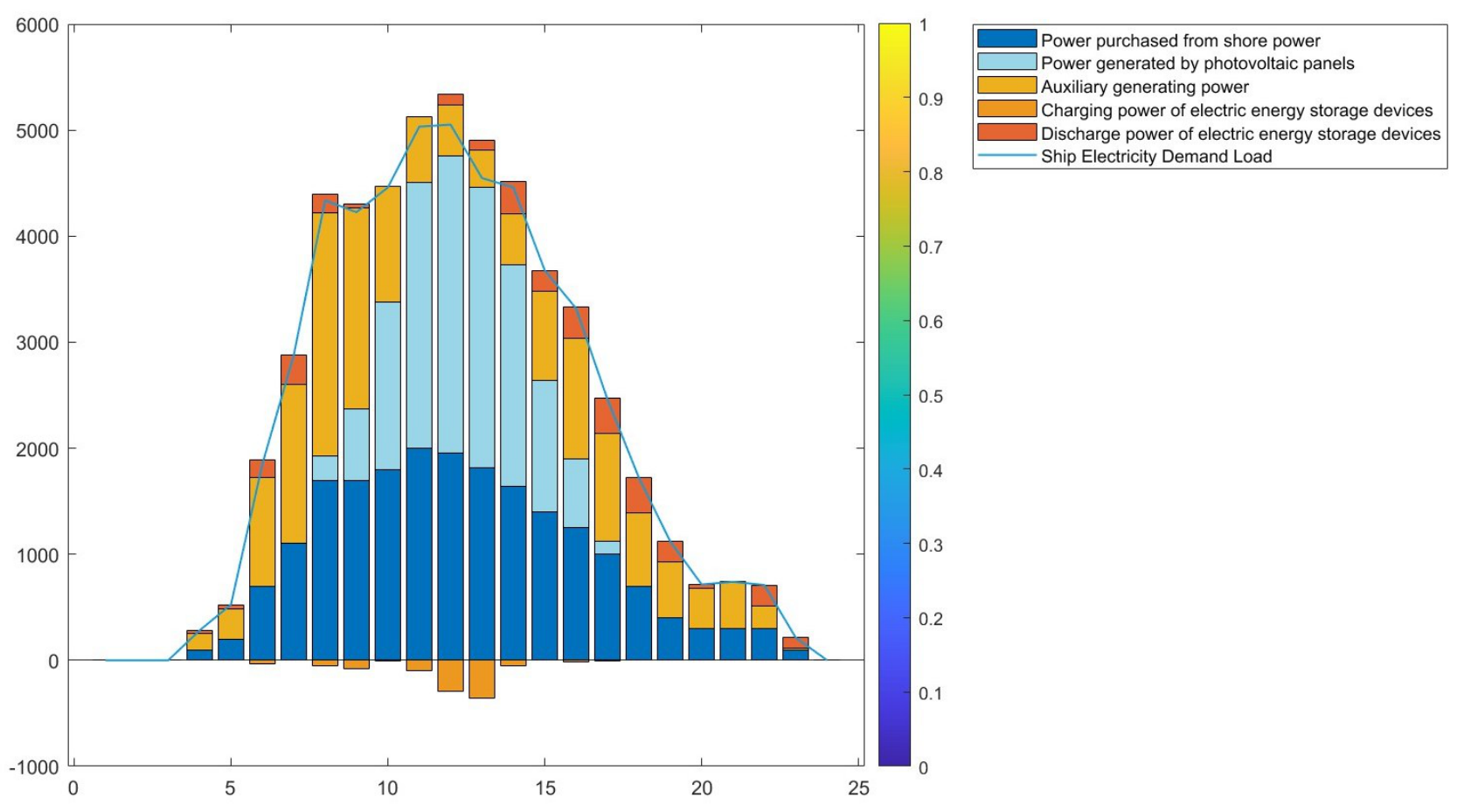
The berth-vessel planning model supplies ship electricity demand during port stays while minimizing energy-use cost. It coordinates onboard storage, auxiliary engines, photovoltaic panels, and port shore-power facilities. Figure 12 reports the output of vessel-side devices, and Figure 13 shows the corresponding power balance. The first group of ships arrives around 4:00 AM, after which shore-power demand gradually increases. Early in the berthing period, photovoltaic output is limited, so shore power and auxiliary generation provide most of the supply. As irradiance rises, onboard photovoltaic generation contributes more electricity and reduces reliance on auxiliary engines and shore power.
Figure 13 indicates that shore power, auxiliary generation, photovoltaic output, and storage operation jointly satisfy vessel-side demand during berthing.
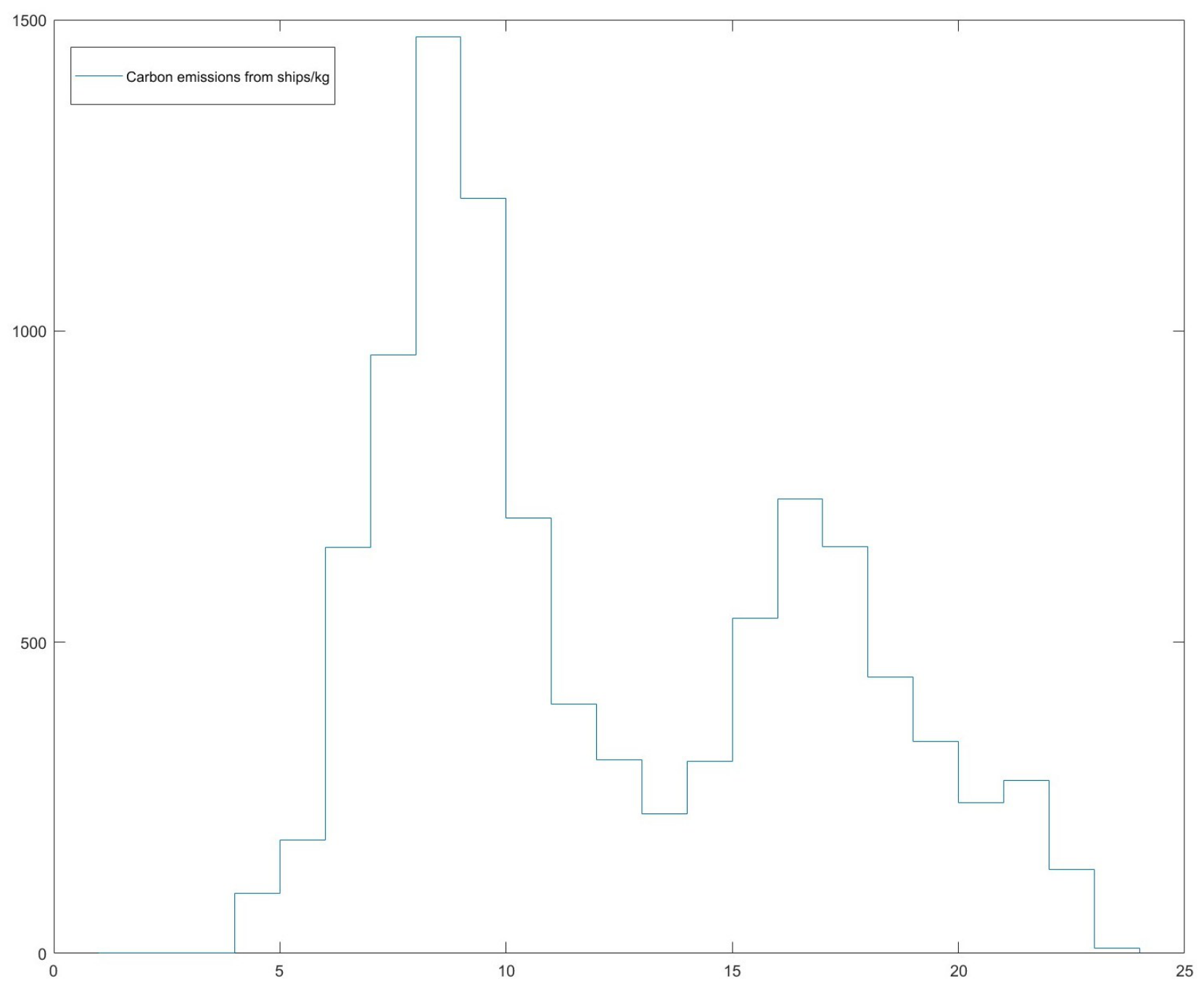
Figure 14 gives the carbon-emission trajectory of ships during berthing and shows how ship-side scheduling affects auxiliary-engine emissions. Emissions start at 4:00 AM when the first ships arrive. As more ships berth, emissions increase quickly, especially between 7:00 AM and 10:00 AM. After 10:00 AM, photovoltaic output rises and replaces part of auxiliary-engine generation, so emissions begin to fall. In the evening, departures reduce the number of berthed vessels, causing emissions to decline further. This pattern shows that integrated scheduling can maintain ship-side energy supply while reducing auxiliary-engine emissions.

5.5. Impact of Five-Tier Carbon Trading Penalty Mechanism Parameters on System Low-Carbon Dispatching

Carbon quota-trading settings directly affect equipment dispatch and total operating cost. In this study, the carbon-trading base price and tier-interval length are treated as policy-intensity parameters. Their effects are examined through simulation rather than imposed as fixed regulatory values. The simulations therefore evaluate how the tiered carbon-trading mechanism changes both low-carbon and economic operation.

5.5.1. Analysis of the Impact of Carbon Trading Base Prices on the System

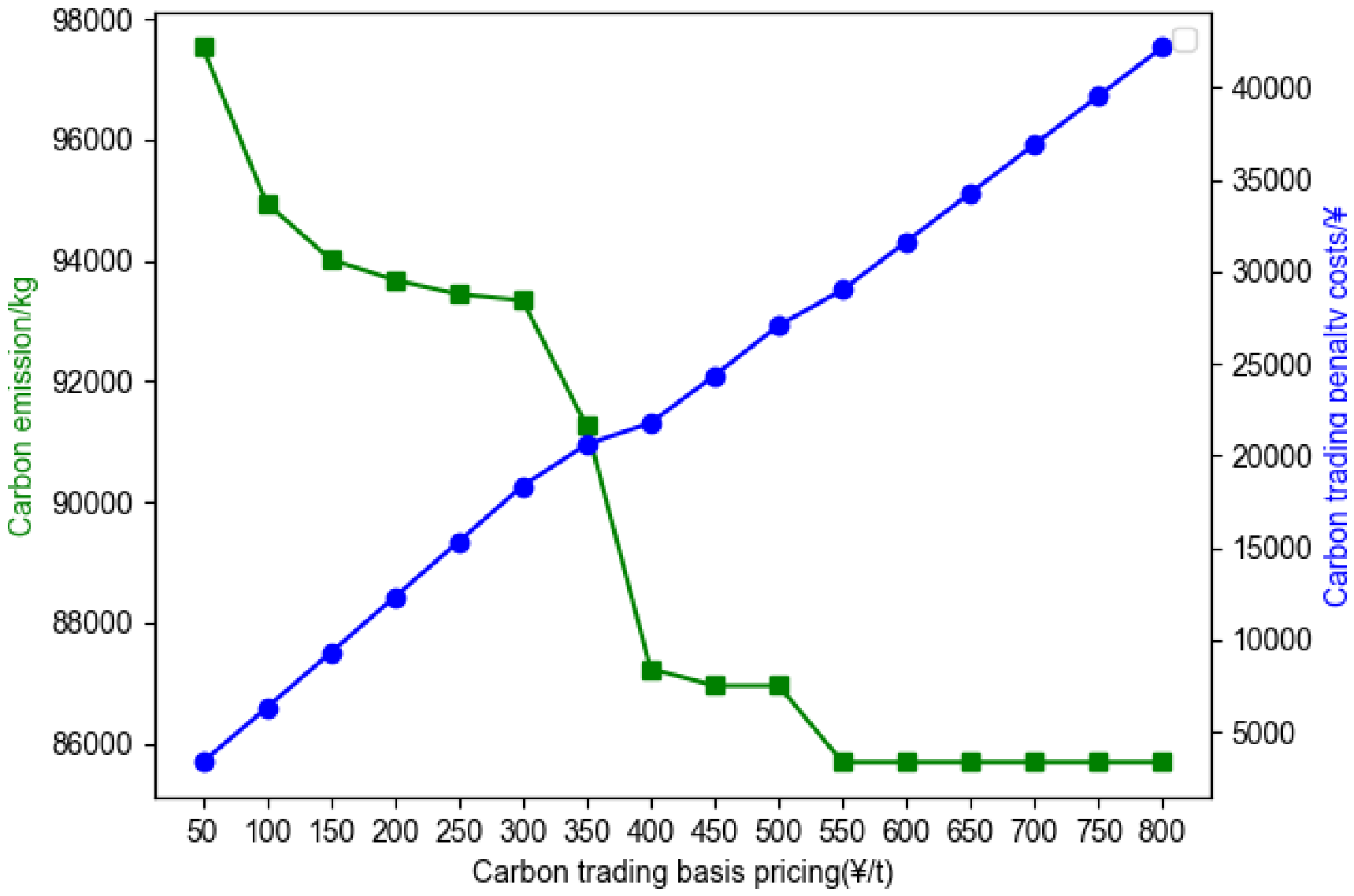
Figure 15 examines the effect of the carbon-trading base price on carbon emissions and carbon-trading cost.
As Figure 15 shows, the carbon-trading base price influences both actual emissions and carbon-trading cost. When the base price is low, carbon cost has a limited effect on the objective function, so the incentive to reduce emissions is weak. As the base price rises, lower-emission dispatch becomes more attractive, and the system adjusts equipment output to reduce actual emissions. The reduction is bounded by technical and operational constraints; after that boundary is approached, further price increases bring only small emission reductions while carbon cost continues to rise.
Thus, carbon price, emissions, and carbon cost interact nonlinearly. A higher base price can promote emission reduction, but beyond a certain range the marginal emission-reduction effect weakens and the economic burden becomes more evident.

5.5.2. Impact Analysis of Changes in Tiered Trading Interval Lengths

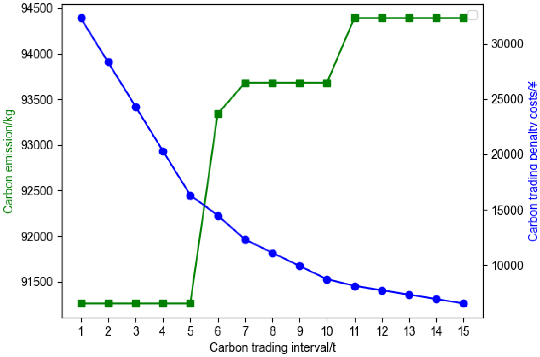
Figure 16 evaluates how tier-interval length changes emission-reduction incentives and carbon-trading cost.
As Figure 16 shows, a shorter tier interval makes excess emissions enter higher price tiers sooner, increasing carbon-trading cost and strengthening low-carbon dispatch pressure. When the interval length is within ( 1 , 5 ] t, the narrow interval keeps marginal penalties high and encourages relatively low emissions. When the interval length is within ( 5 , 9 ] t, the same emission level falls into lower marginal tiers, so carbon cost decreases and the incentive to reduce emissions weakens. Once the interval length exceeds 9 t, further increases have limited influence because most excess emissions remain in lower-price intervals.
Appropriate base prices and tier-interval lengths are therefore important for balancing economic and low-carbon performance. Well-chosen parameters can reduce emissions without creating excessive operating cost. In practical port applications, such a mechanism would require reliable emission accounting, real-time energy monitoring, and consistency with local carbon-market rules. The parameter analysis in this paper should therefore be viewed as a mechanism-oriented simulation rather than a direct policy prescription.

5.6. Comparative Analysis of ADN Schedule Operation Plans Under Different Scenarios

To verify the ADN scheduling strategy, four scenarios are compared by changing only whether demand response and the tiered carbon-penalty mechanism are activated:
Scenario 1: the base case, in which neither demand response nor the tiered carbon-penalty mechanism is used as a dispatch signal;
Scenario 2: the demand response case, in which only demand response is activated and the load profile is adjusted according to the optimized time-of-use price response;
Scenario 3: the carbon-penalty case, in which only the tiered carbon-penalty mechanism is activated and excess emissions are internalized in dispatch cost;
Scenario 4: the combined case, in which demand response and the tiered carbon-penalty mechanism are both activated.
For comparability, all other settings remain unchanged across the four scenarios, including equipment capacities, unit costs, conversion efficiencies, renewable-generation profiles, vessel and vehicle quantities, initial load demand, operating constraints, and solver settings. The differences in cost, energy purchases, and emissions therefore mainly reflect demand response, the carbon penalty, and their combined effect. Carbon-related cost is reported in all scenarios, but it acts as an active dispatch signal only when the tiered carbon-penalty mechanism is enabled.
Although ship auxiliary-engine emissions are included in the five-tier carbon-penalty mechanism, auxiliary-engine schedules are mainly constrained by shore-power availability and onboard planning. The tiered penalty therefore mainly internalizes environmental cost in the optimization rather than directly controlling auxiliary-engine operation, ensuring that port-side dispatch accounts for all emission sources in the economic evaluation.
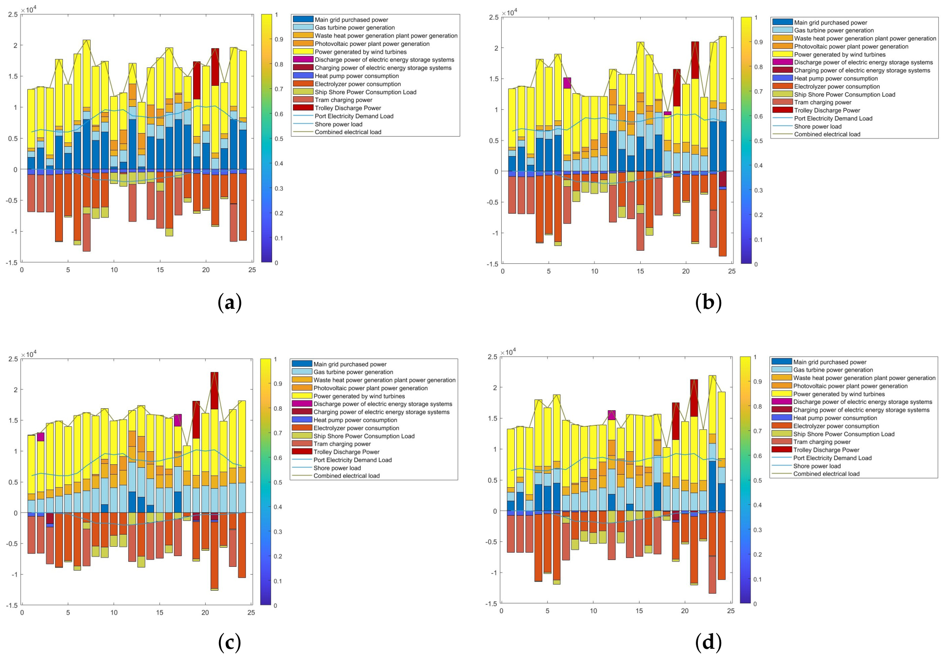
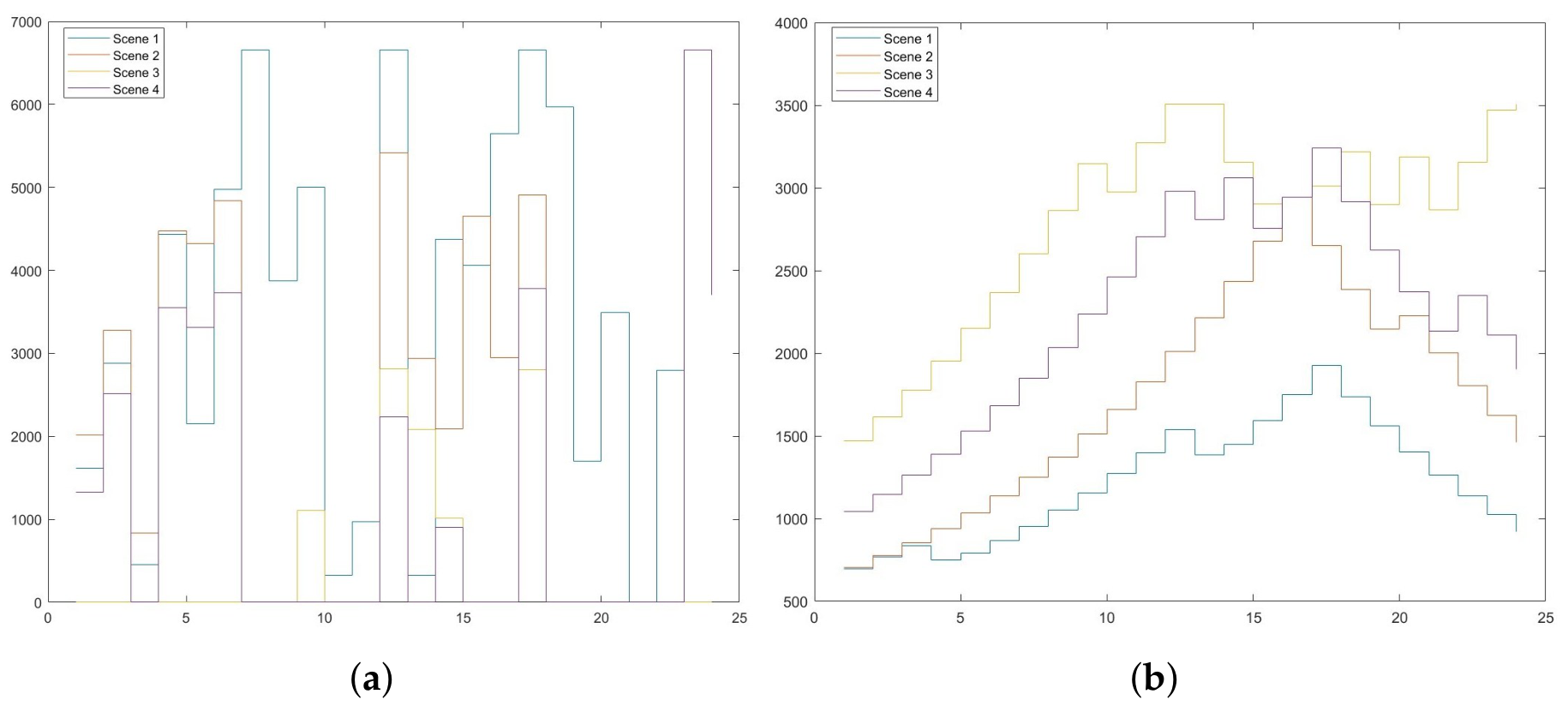
Table 7, Table 8 and Table 9 compare total system cost, energy purchase cost, and low-carbon performance across the four scenarios. Figure 17 and Figure 18 show the corresponding electric power balance and carbon-emission changes. The comparison between Scenarios 1 and 2 isolates the demand response effect. In Scenario 2, time-of-use prices reshape electricity consumption, reduce high-price grid purchases, and shift part of the load to lower-price periods. Although equipment usage and some vehicle costs rise slightly, the energy purchase structure improves. Comparing Scenarios 1 and 4 shows that jointly applying demand response and the carbon penalty provides the lowest total dispatch cost among the tested cases.
In the scenario comparison, their cost contribution is reflected in Table 9, while emission reduction remains limited by ship-side constraints.
The comparison between Scenarios 1 and 3 highlights the role of the tiered carbon penalty. Once this mechanism is introduced, the energy-consumption pattern changes. Figure 17a,c show that grid electricity purchases decrease substantially, while CHP utilization increases. This indicates that the model shifts toward lower-carbon and more cost-effective energy conversion when carbon penalties are internalized.
Greater CHP utilization helps satisfy coupled electricity and heat demand while reducing total emissions. Lower emissions directly reduce tiered penalty expenses. Compared with Scenario 1, Scenario 3 reduces carbon emissions by 8.59 tons and saves 24,038.40 yuan, confirming that an appropriate environmental-cost signal can guide the system toward cleaner dispatch.
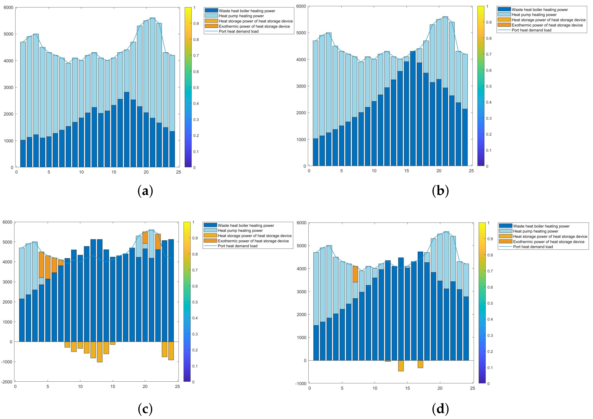
The scenario comparison also shows that the CHP structure supports coordinated electricity–heat scheduling. As illustrated in Figure 17 and Figure 19c,d, introducing the carbon penalty increases CHP utilization and strengthens waste-heat recovery in thermal supply. Because system thermal balance depends closely on CHP output, optimized CHP operation improves heat-supply efficiency and emission performance. Scenario 4 further balances economic dispatch, renewable utilization, and emission reduction.
Among the four scenarios, Scenario 4 combines the advantages of demand response and tiered carbon-trading penalties. Relative to Scenario 1, carbon emissions fall by 30,915.43 kg, or approximately 24.52 % , and economic dispatch cost decreases by 31,035.92 yuan, or about 11.05 % . These results show that the proposed strategy can reduce emissions while maintaining stable and economical port microgrid operation.

6. Results Summary and Validation

The four scenario results validate the proposed port energy management model from cost, energy-purchase, and emission perspectives. Jointly applying demand response and the tiered carbon-penalty mechanism reduces electricity purchases, improves the use of CHP and renewable resources, and lowers carbon emissions while preserving operational feasibility. The findings are consistent with prior integrated energy-system studies [40,42], which show that demand response, EV charging optimization, and carbon-cost mechanisms can improve economic and environmental performance. Differences from previous benchmarks mainly arise from the case-study scale, the inclusion of hydrogen heavy-duty vehicles, and port-specific operating constraints. Hourly load fluctuations are explained by vessel arrival randomness and variable renewable generation, both of which are included in the simulation. The results confirm that the proposed model captures key port energy-management dynamics and can support operational planning and policy analysis.

7. Conclusions

Power-system reform and the development of renewable energy, storage, and demand response technologies provide ports with stronger technical support for low-carbon transformation. This paper proposes an integrated port energy management model that includes the energy demand of ships and heavy-duty vehicles. The model coordinates renewable generation, hydrogen production and storage, shore power, vehicle scheduling, demand response, and tiered carbon penalties to improve economic and environmental performance. The main conclusions are as follows:
  • A Logistic-function-based demand response model is developed for price optimization. With user satisfaction and load fluctuation as the two objectives, multi-objective particle swarm optimization identifies feasible trade-off solutions and links them with dynamic charging/discharging prices for electric heavy-duty vehicles.
  • A hydrogen production–storage–use framework is constructed for port-area hydrogen demand. Renewable electricity is converted into hydrogen through electrolysis, stored, and supplied to hydrogen heavy-duty vehicles, supporting cleaner vehicle operation and increasing renewable-energy utilization.
  • Free carbon allowances are assigned using the baseline method, and actual emissions are calculated from dispatch results. The tiered carbon-trading penalty then guides the system toward lower-emission energy use while maintaining economic feasibility.
This study focuses on grid-connected integrated energy management and provides a basis for daily port dispatch. In broader applications, especially isolated-island ports or weak-grid environments, essential operation under limited external energy support may be more difficult. Future research will therefore examine islanded operation, storage autonomy, and resilient scheduling under extreme or grid-disconnected conditions.
Future work will also explore how to improve energy-use efficiency while ensuring continuous port operation, reducing waste, and securing long-term sustainable energy supply. More flexible and intelligent integrated energy management systems can strengthen port resilience and self-sufficiency under uncertain renewable output, variable logistics demand, and extreme operating scenarios.

Author Contributions

Conceptualization, G.Y. and H.H.; methodology, G.Y. and H.N.; software, G.Y. and R.W.; validation, G.Y., H.N. and R.W.; formal analysis, G.Y.; investigation, G.Y.; resources, H.H.; data curation, G.Y.; writing—original draft preparation, G.Y.; writing—review and editing, H.H. and D.P.; visualization, G.Y.; supervision, H.H.; project administration, H.H.; funding acquisition, H.H. All authors have read and agreed to the published version of the manuscript.

Funding

This research was funded by Shanghai University of Political Science and Law, grant number 2026XYB01.

Institutional Review Board Statement

Not applicable.

Informed Consent Statement

Not applicable.

Data Availability Statement

The data used in the numerical simulation are available from the corresponding author upon reasonable request.

Conflicts of Interest

The authors declare no conflicts of interest.

Abbreviations

The following abbreviations are used in this manuscript:
ADNActive Distribution Network
CHPCombined Heat and Power
CICold Ironing
DRDemand Response
EESElectrical Energy Storage
HESHydrogen Energy Storage
HPHeat Pump
MTMicro Turbine
ORCOrganic Rankine Cycle
PVPhotovoltaic
SOCState of Charge
TESThermal Energy Storage
WHBWaste Heat Boiler
WTWind Turbine

References

  1. Parvasi, S.P.; Panagakos, G.; Barfod, M.B.; Lam, J.S.L. Ports as Energy Hubs: Renewable Energy Integration and Distribution. In Proceedings of the 25th DNV Nordic Maritime Universities Workshop, Kgs. Lyngby, Denmark, 30 January 2025. [Google Scholar]
  2. Peng, S.-T.; Qi, Z.-Y.; Liu, Y.-Y.; Liu, Z.-F.; Li, L.-L. Improving the energy efficiency and economic benefits of port integrated energy systems: A multi-objective optimization model for wind-storage-charging-discharging power stations with green efficiency factors-driven multilateral response strategy. Energy 2025, 339, 138939. [Google Scholar]
  3. Tang, D.; Ge, P.; Yuan, C.; Ren, H.; Zhong, X.; Dong, M.; Agundis-Tinajero, G.D.; Diaz-Londono, C.; Guerrero, J.M.; Zio, E. Optimal management of coupled hydrogen-electricity energy systems at ports by multi-time scale scheduling. Appl. Energy 2025, 391, 125885. [Google Scholar]
  4. Lv, W.; Ye, Y.; Cui, T.; Chen, S.; Xu, D.; Yu, W.; Huang, D.; Liu, Z.; Zhu, J.; Li, T.; et al. Sustainable electrified seaports: A coordinated energy and logistics scheduling approach for future maritime hubs. Appl. Energy 2025, 401, 126645. [Google Scholar] [CrossRef]
  5. Zhang, Y.; Liang, C.; Shi, J.; Lim, G.; Wu, Y. Optimal Port Microgrid Scheduling Incorporating Onshore Power Supply and Berth Allocation Under Uncertainty. Appl. Energy 2022, 313, 118856. [Google Scholar] [CrossRef]
  6. Chen, X.; Bai, R.; Qu, R.; Dong, H.; Chen, J. A data-driven genetic programming heuristic for real-world dynamic seaport container terminal truck dispatching. In Proceedings of the 2020 IEEE Congress on Evolutionary Computation (CEC), Glasgow, UK, 19–24 July 2020; pp. 1–8. [Google Scholar]
  7. Chen, X.; Bai, R.; Qu, R.; Dong, H. Cooperative double-layer genetic programming hyper-heuristic for online container terminal truck dispatching. IEEE Trans. Evol. Comput. 2022, 27, 1220–1234. [Google Scholar]
  8. Xu, B.; Wang, Y.; Li, J. Optimization of port emergency materials dispatch with time windows constraints under uncertainties. Discret. Dyn. Nat. Soc. 2021, 2021, 3977984. [Google Scholar] [CrossRef]
  9. Li, H.; Li, J.; An, L.; Zhang, X.; Xu, Z.; Hu, J. A dispatching method for automated container terminals: What is next when precise execution is available? In Proceedings of the 2023 IEEE 26th International Conference on Intelligent Transportation Systems (ITSC), Bilbao, Spain, 24–28 September 2023; pp. 2434–2439. [Google Scholar]
  10. Deng, Y.; Chen, Y.; Huang, J.; Zhang, D.; Zhao, J. A two-stage routing optimization model for yard trailers in container terminals under stochastic demand. Evol. Intell. 2023, 16, 1853–1863. [Google Scholar]
  11. Hsu, H.-P.; Chou, C.-C.; Wang, C.-N. Heuristic/metaheuristic-based simulation optimization approaches for integrated scheduling of yard crane, yard truck, and quay crane considering import and export containers. IEEE Access 2022, 10, 64650–64670. [Google Scholar]
  12. Zhen, L.; Lv, W.; Tan, Z.; Dong, B. Container transportation scheduling between port yards and the hinterland in Yunfeng. Inf. J. Appl. Anal. 2022, 52, 250–266. [Google Scholar] [CrossRef]
  13. Hou, J.; Song, Z.; Hofmann, H.; Sun, J. Adaptive model predictive control for hybrid energy storage energy management in all-electric ship microgrids. Energy Convers. Manag. 2019, 198, 111929. [Google Scholar] [CrossRef]
  14. Li, Z.; Xu, Y.; Wu, L.; Zheng, X. A risk-averse adaptively stochastic optimization method for multi-energy ship operation under diverse uncertainties. IEEE Trans. Power Syst. 2020, 36, 2149–2161. [Google Scholar]
  15. Edrington, C.S.; Ozkan, G.; Papari, B.; Gonsoulin, D.E.; Perkins, D.; Vu, T.V.; Vahedi, H. Distributed energy management for ship power systems with distributed energy storage. J. Mar. Eng. Technol. 2020, 19, 31–44. [Google Scholar]
  16. Hein, K.; Yan, X.; Wilson, G. Multi-objective optimal scheduling of a hybrid ferry with shore-to-ship power supply considering energy storage degradation. Electronics 2020, 9, 849. [Google Scholar]
  17. Xu, L.; Wen, Y.; Luo, X.; Lu, Z.; Guan, X. A modified power management algorithm with energy efficiency and GHG emissions limitation for hybrid power ship system. Appl. Energy 2022, 317, 119114. [Google Scholar] [CrossRef]
  18. Hein, K. Emission-aware and data-driven many-objective voyage and energy management optimization of solar-integrated all-electric ship. Electr. Power Syst. Res. 2022, 213, 108718. [Google Scholar]
  19. Wang, Z.; Ma, Y.; Sun, Y.; Tang, H.; Cao, M.; Xia, R.; Han, F. Optimizing energy management and case study of multi-energy coupled supply for green ships. J. Mar. Sci. Eng. 2023, 11, 1286. [Google Scholar] [CrossRef]
  20. Li, Z.; Xu, Y.; Fang, S.; Wang, Y.; Zheng, X. Multiobjective coordinated energy dispatch and voyage scheduling for a multienergy ship microgrid. IEEE Trans. Ind. Appl. 2019, 56, 989–999. [Google Scholar] [CrossRef]
  21. Taheri, S.I.; Vieira, G.G.T.T.; Salles, M.B.C.; Avila, S.L. A trip-ahead strategy for optimal energy dispatch in ship power systems. Electr. Power Syst. Res. 2021, 192, 106917. [Google Scholar] [CrossRef]
  22. Wen, S.; Zhao, T.; Tang, Y.; Xu, Y.; Zhu, M.; Fang, S.; Ding, Z. Coordinated optimal energy management and voyage scheduling for all-electric ships based on predicted shore-side electricity price. IEEE Trans. Ind. Appl. 2020, 57, 139–148. [Google Scholar]
  23. Huang, W.; Yu, M.; Li, H.; Tai, N. Energy Management of Integrated Energy System in Large Ports; Springer Nature: Singapore, 2023. [Google Scholar]
  24. Iris, Ç.; Lam, J.S.L. Optimal energy management and operations planning in seaports with smart grid while harnessing renewable energy under uncertainty. Omega 2021, 103, 102445. [Google Scholar] [CrossRef]
  25. Wang, X.; Huang, W.; Wei, W.; Tai, N.; Li, R.; Huang, Y. Day-ahead optimal economic dispatching of integrated port energy systems considering hydrogen. IEEE Trans. Ind. Appl. 2021, 58, 2619–2629. [Google Scholar] [CrossRef]
  26. Lasseter, R.; Akhil, A.; Marnay, C.; Stephens, J.; Dagle, J.; Guttromson, R.; Meliopoulous, A.; Yinger, R.; Eto, J. The CERTS microgrid concept. White Pap. Transm. Reliab. Program Off. Power Technol. U.S. Dep. Energy 2002, 2, 30. [Google Scholar]
  27. Parra, D.; Norman, S.A.; Walker, G.S.; Gillott, M. Optimum community energy storage system for demand load shifting. Appl. Energy 2016, 174, 130–143. [Google Scholar] [CrossRef]
  28. Krishnamurthy, D.; Uckun, C.; Zhou, Z.; Thimmapuram, P.R.; Botterud, A. Energy storage arbitrage under day-ahead and real-time price uncertainty. IEEE Trans. Power Syst. 2017, 33, 84–93. [Google Scholar]
  29. Das, C.K.; Bass, O.; Mahmoud, T.S.; Kothapalli, G.; Mousavi, N.; Habibi, D.; Masoum, M.A.S. Optimal allocation of distributed energy storage systems to improve performance and power quality of distribution networks. Appl. Energy 2019, 252, 113468. [Google Scholar] [CrossRef]
  30. Rajamand, S.; Shafie-khah, M.; Catalão, J.P.S. Energy storage systems implementation and photovoltaic output prediction for cost minimization of a microgrid. Electr. Power Syst. Res. 2022, 202, 107596. [Google Scholar] [CrossRef]
  31. Kavousi-Fard, A.; Khorram-Nia, R.; Rostami, M.; Abbasi, A. An smart stochastic approach to model plug-in hybrid electric vehicles charging effect in the optimal operation of micro-grids. J. Intell. Fuzzy Syst. 2015, 28, 835–842. [Google Scholar] [CrossRef]
  32. Pimm, A.J.; Cockerill, T.T.; Taylor, P.G. The potential for peak shaving on low voltage distribution networks using electricity storage. J. Energy Storage 2018, 16, 231–242. [Google Scholar] [CrossRef]
  33. Fang, S.; Wang, C.; Liao, R.; Zhao, C. Optimal power scheduling of seaport microgrids with flexible logistic loads. IET Renew. Power Gener. 2022, 16, 2711–2720. [Google Scholar] [CrossRef]
  34. Tao, Y.; Qiu, J.; Lai, S.; Sun, X.; Zhao, J. Flexible voyage scheduling and coordinated energy management strategy of all-electric ships and seaport microgrid. IEEE Trans. Intell. Transp. Syst. 2022, 24, 3211–3222. [Google Scholar] [CrossRef]
  35. Ban, Z.; Teng, F.; Zhang, H.; Li, S.; Xiao, G.; Guan, Y. Distributed fixed-time energy management for port microgrid considering transmissive efficiency. Mathematics 2023, 11, 3674. [Google Scholar] [CrossRef]
  36. Bakar, N.N.A.; Guerrero, J.M.; Vasquez, J.C.; Bazmohammadi, N.; Othman, M.; Rasmussen, B.D.; Al-Turki, Y.A. Optimal configuration and sizing of seaport microgrids including renewable energy and cold ironing—The Port of Aalborg case study. Energies 2022, 15, 431. [Google Scholar] [CrossRef]
  37. Teng, F.; Wang, J.; Luo, H.; Zhang, Q.; Shen, C. Distributed low-carbon energy management method for port microgrid based on we-energies under polymorphic network. Front. Energy Res. 2022, 10, 952396. [Google Scholar]
  38. Shan, Q.; Song, J.; Xu, Q.; Xiao, G.; Yu, F. Polymorphic distributed energy management for low-carbon port microgrid with carbon capture and carbon storage devices. Front. Energy Res. 2022, 10, 951192. [Google Scholar] [CrossRef]
  39. Song, J.; Shan, Q.; Zou, T.; Hu, J.; Teng, F. Distributed energy management for zero-carbon port microgrid. Int. Trans. Electr. Energy Syst. 2022, 2022, 2752802. [Google Scholar] [CrossRef]
  40. Wu, H.; Qiu, D.; Zhang, L.; Sun, M. Adaptive multi-agent reinforcement learning for flexible resource management in a virtual power plant with dynamic participating multi-energy buildings. Appl. Energy 2024, 374, 123998. [Google Scholar]
  41. Zhang, Z.; Yu, D. RBF-NN based short-term load forecasting model considering comprehensive factors affecting demand response. Proc. CSEE 2018, 38, 1631–1638. [Google Scholar]
  42. Ma, M.; Wei, W.; Li, L. Two-stage robust optimal scheduling of a microgrid with a stepped carbon trading mechanism. Power Syst. Prot. Control 2023, 51, 22–33. [Google Scholar]
  43. Saint-Drenan, Y.-M.; Besseau, R.; Jansen, M.; Staffell, I.; Troccoli, A.; Dubus, L.; Schmidt, J.; Gruber, K.; Simões, S.G.; Heier, S. A parametric model for wind turbine power curves incorporating environmental conditions. Renew. Energy 2020, 157, 754–768. [Google Scholar] [CrossRef]
  44. Huang, X.; Chen, J.; Xie, Q.; Cao, Y.; Yang, H. The influence of users’ charging selection on charging schedule of power grid. Trans. China Electrotech. Soc. 2018, 33, 3002–3011. [Google Scholar]
  45. Gao, H.; Liu, J.; Shen, X.; Xu, R. Optimal power flow research in active distribution network and its application examples. Proc. CSEE 2017, 37, 1634–1644. [Google Scholar]
Figure 1. Workflow of the proposed port energy management study.
Energies 19 02970 g001
Figure 2. Interaction mechanism among port logistics loads, multi-energy supply, demand response, and carbon-cost signals.
Energies 19 02970 g002
Figure 3. Load-transfer response under different peak-to-valley price differentials.
Energies 19 02970 g003
Figure 4. Pareto frontier of the demand response optimization.
Energies 19 02970 g004
Figure 5. Price and load profiles before and after applying demand response.
Energies 19 02970 g005
Figure 6. Original and optimized charging/discharging prices for electric heavy-duty vehicles.
Energies 19 02970 g006
Figure 7. Electric-vehicle operation states before and after pricing optimization. (a) Electric-vehicle operating states before pricing optimization; (b) Electric-vehicle operating states after pricing optimization.
Energies 19 02970 g007
Figure 8. State-of-charge (SOC) trajectories of electric heavy-duty vehicles under pricing optimization. (a) SOC trajectories before pricing optimization; (b) SOC trajectories after pricing optimization.
Energies 19 02970 g008
Figure 9. Electrolyzer power consumption during the scheduling horizon.
Energies 19 02970 g009
Figure 10. Hydrogen storage state over 24 h.
Energies 19 02970 g010
Figure 11. Operating states and hydrogen-tank levels of hydrogen heavy-duty vehicles. (a) Discrete operating states of hydrogen heavy-duty vehicles, including transportation, hydrogen refueling, and idle modes; (b) Temporal evolution of hydrogen-tank state-of-energy under vehicle operation and refueling scheduling.
Energies 19 02970 g011
Figure 12. Output of vessel-side energy devices over a 24-h period. (a) Net power balance of ship-side energy storage and load demand; (b) Shore power supply profile during berth periods; (c) Auxiliary engine power output under varying shore power and photovoltaic availability; (d) Shipboard photovoltaic power generation contributing to vessel energy demand.
Energies 19 02970 g012
Figure 13. Vessel-side power balance during berthing over 24 h.
Energies 19 02970 g013
Figure 14. Ship berthing carbon emissions over 24 h.
Energies 19 02970 g014
Figure 15. Effect of carbon-trading base price changes on system emissions and cost.
Energies 19 02970 g015
Figure 16. Effect of tier-interval length changes on system emissions and carbon cost.
Energies 19 02970 g016
Figure 17. Port electric power balance under different operating scenarios. (a) Baseline scenario without demand response or carbon-penalty mechanism; (b) Scenario with demand response enabled; (c) Integrated scenario with demand response and tiered carbon-trading penalty; (d) Fully coordinated optimization scenario considering renewable integration, demand response, and carbon constraints.
Energies 19 02970 g017
Figure 18. Comparison of port carbon emissions from electricity and gas consumption under different operating scenarios. (a) Carbon emissions associated with electricity consumption from grid power and electricity-based processes under Scenarios 1–4; (b) Carbon emissions associated with gas consumption and CHP-related energy conversion under Scenarios 1–4.
Energies 19 02970 g018
Figure 19. Thermal power balance of the port integrated energy system under different operating scenarios. (a) Baseline thermal energy balance dominated by conventional CHP and heat supply units; (b) Thermal dispatch with increased renewable and heat pump participation; (c) Thermal energy redistribution under demand response and tiered carbon-trading penalty; (d) Fully coordinated optimization scenario with integrated multi-energy coupling and carbon-aware thermal dispatch.
Energies 19 02970 g019
Table 1. Port equipment parameters.
Equipment NameFundamental Parameter NameValueEconomic Parameter (RMB/kWh)
MTPower output limits/kW
Electric efficiency
Thermal efficiency
Ramp rate limits
4800/0
0.3
0.6
0.1/−0.1
0.15
ORCPower output limits/kW
Electric efficiency
3200/0
0.8
0.25
WHBPower output limits/kW
Thermal efficiency
6400/0
0.8
0.28
HPPower output limits/kW
Conversion factor
900/0
4.2
0.15
EESCapacity/kWh
Power output limits/kW
9600
3200/−3200
0.11
TESCapacity/kWh
Power output limits/kW
5200
1300/−1300
0.12
HESCapacity/kWh
Power output limits/kW
1500
300/−300
0.26
PVPower output limits/kW10,800/00.20
WTPower output limits/kW3600/00.13
EleEfficiency0.60.25
CIUpper and lower limits of unit output/kW100/0/
Table 2. Vessel parameters.
InstallationsParametersNumerical Value
AGPower output limits/kW
Unit price (RMB/kg)
150/0
1.172
PVPower output limits/kW200/0
EESCapacity/kWh
Power output limits/kW
5000
100/−100
Table 3. Parameters of hydrogen load transportation vehicles.
NameNumerical ValueUnit
Capacity50kg
Maximum and minimum state of charge0.9/0.1/
Number of hydrogen vehicles20vehicle
Total carrying capacity300TEUs
Operational state3/
Table 4. Parameters of electric heavy-duty transportation vehicles.
NameNumerical ValueUnit
Capacity500kg
Maximum and minimum state of charge0.9/0.1/
Number of electric vehicles40vehicle
Total carrying capacity400TEUs
Operational state4/
Table 5. Customer satisfaction and load volatility before and after demand response.
StateCustomer SatisfactionLoad Volatility
Before demand response1.001.35
After demand response0.870.91
Table 6. Electric-vehicle energy-use cost with and without pricing optimization.
Availability of Tariff Optimization StrategiesCharging Cost/RMBDischarge Proceeds/RMBTotal Energy Use Cost/RMB
Not available35,70012,90022,800
Available38,390.59719,578.1318,812.44
Table 7. Cost impacts on the port integrated energy system under different scenarios.
ScenarioEnergy PurchaseCarbon PenaltyEquipment Usage CostVesselVehicleTotal Cost
1106,896.3344,459.37129,602.2936,103.5865,218.49382,280.05
286,070.9585,648.48137,336.3336,103.5866,332.44411,491.77
386,236.1220,420.97154,025.1836,103.5865,218.49362,004.33
480,391.0125,315.58144,215.4736,103.5866,332.44352,358.09
Table 8. Port energy purchase costs under different scenarios.
ScenarioMain Grid
Power Purchase
Purchase of GasTotal Cost of
Energy Purchased
173,149.9133,746.41106,896.33
237,983.7248,087.2386,070.95
38271.1677,964.9686,236.12
418,575.0161,816.0080,391.01
Table 9. Low-carbon characteristics of the port energy system under different scenarios.
ScenarioTotal Cost of Energy Purchased/RMBActual Carbon Emissions/kg
144,459.37126,058.61
285,648.48107,577.80
320,420.9787,238.83
425,315.5895,143.18
Disclaimer/Publisher’s Note: The statements, opinions and data contained in all publications are solely those of the individual author(s) and contributor(s) and not of MDPI and/or the editor(s). MDPI and/or the editor(s) disclaim responsibility for any injury to people or property resulting from any ideas, methods, instructions or products referred to in the content.