Article

Type-2 Fuzzy C-Means-Based Clustering-Decomposed Coordination of Directional Overcurrent Relays

1
Department of Data Science and AI, Faculty of Information Technology, Monash University, Melbourne, VIC 3800, Australia
2
Department of Electrical Engineering, COMSATS University Islamabad, Islamabad 45550, Pakistan
3
Department of Electrical Engineering, COMSATS University Islamabad, Attock Campus, Attock 43600, Pakistan
4
School of Engineering, Swinburne University of Technology, Melbourne, VIC 3122, Australia
*
Authors to whom correspondence should be addressed.
Energies 2026, 19(12), 2943; https://doi.org/10.3390/en19122943
Submission received: 10 May 2026 / Revised: 14 June 2026 / Accepted: 18 June 2026 / Published: 22 June 2026
(This article belongs to the Special Issue Optimization and Machine Learning Approaches for Power Systems)

Abstract

Optimal coordination of directional overcurrent relays (DOCRs) in medium-to-large power systems constitutes a computationally demanding, mixed-integer, nonlinear optimisation problem whose complexity escalates rapidly with system size, making the simultaneous minimisation of relay operating time and computational cost a critical open challenge. This study presents a two-level hierarchical framework in which Type-2 Fuzzy C-Means (T2FCM) clustering partitions 226 fault scenarios into subproblems at the upper level, while the Hybrid Fractional Entropy Evolution (HFEE) algorithm independently optimises relay settings for each cluster at the lower level. HFEE integrates fractional-order velocity updates—derived from the Grünwald–Letnikov formulation—with a Shannon entropy diversity-control mechanism to prevent premature convergence. T2FCM captures inherent fault-current uncertainty through interval-valued type-2 fuzzy memberships, yielding more robust cluster assignments near protection-zone boundaries than crisp partitioning methods. The framework is validated on the extended IEEE 30-bus system. An ablation study demonstrates that standalone HFEE achieves a 29.19% improvement in T op over the prior best-reported result; however, a comprehensive parameter sweep over cluster counts K { 2 , , 8 } and fractional orders α { 0.1 , , 0.9 } across 50 independent runs per configuration shows that the proposed clustering-decomposed method achieves 3.68–66.67% lower wall-clock computation time while maintaining zero CTI violations across all active relay pairs. The communicationless, entirely offline framework demonstrates scalability for simultaneous sub-transmission and distribution protection coordination and offers a practically deployable strategy for modern power networks.

1. Introduction

In modern power systems, directional overcurrent relays (DOCRs) form the primary line of defence for isolating faulted segments while preserving the continuity of supply in healthy zones. These relays detect fault current magnitude and direction, making their coordinated operation fundamental to network stability and reliability [1,2,3]. DOCR coordination requires the simultaneous determination of optimal time multiplier settings (TMS) and plug settings (PS) so that each primary relay trips before its designated backup by a prescribed coordination time interval (CTI), while minimising total relay operating time.
The problem grows considerably more demanding in large-scale networks. The extended IEEE 30-bus system—a representative sub-transmission/distribution benchmark—comprises 81 DOCRs protecting 41 lines and 4 transformers across both 132 kV and 33 kV voltage levels [4,5]. With 162 decision variables (81 TMS and 81 PS) and 226 primary-–backup coordination constraints, the resulting mixed-integer nonlinear program is intractable for purely analytical methods [6].
Conventional solution strategies span deterministic mathematical programming, including sequential quadratic programming (SQP) [7] and mixed-integer linear programming [8], and population-based metaheuristics such as particle swarm optimisation (PSO) [9], gravitational search algorithm (GSA) [10], differential evolution [11,12], firefly algorithm [13], and cuckoo search [14]. Mathematical programming methods offer convergence guarantees but become computationally prohibitive as problem size increases and are prone to entrapment in local optima when discrete PS values are handled alongside continuous TMS variables [15]. Population-based metaheuristics scale better, yet suffer from premature convergence in high-dimensional search spaces [6].
A critical limitation shared by the majority of prior studies is that they are validated exclusively on the reduced 38-relay configuration of the IEEE 30-bus system or on networks with fewer than 120 coordination constraints [7,12,16]. Methods applied to the full 81-relay configuration with 226 constraints are scarce; Abdelaziz et al. [5] solved a linear programming formulation, and Bayazidi et al. [4] employed HEPSO and TFWO, achieving 35.73 s on the extended system while emphasising the practical importance of discrete relay settings. Neither study, however, employs clustering-based decomposition, and no prior work has validated T2FCM clustering on a system with more than 200 coordination constraints.
A complementary research direction has pursued decomposition strategies, partitioning large coordination problems into tractable subproblems. Ojaghi and Mohammadi [17] demonstrated that clustering can reduce the number of distinct setting groups required for adaptive relay coordination. Zand et al. [18] applied clustering-based zero-miscoordination techniques to group network topologies under N-2 contingencies. However, these approaches rely on crisp clustering assignments, which force fault scenarios near protection-zone boundaries into a single cluster and cannot model the measurement uncertainty inherent in fault current data.
Type-2 Fuzzy C-Means (T2FCM) [19] overcomes this limitation through interval-valued memberships [ u ̲ i j , u ¯ i j ] , whose footprint of uncertainty (FOU) captures the ambiguity in scenario-cluster assignment. The authors recently introduced the Hybrid Fractional Entropy Evolution (HFEE) framework. In [20,21], a fractional PSO–GSA with entropy evolution was validated on small IEEE 3-bus and 8-bus systems, achieving approximately 9–12% improvements in operating time over the base PSO–GSA. A subsequent paper [22] extended the framework to IEEE 3-, 8-, and 15-bus networks with 15–26% reductions. Each of those studies, however, optimised the full relay network as a single monolithic problem, which becomes increasingly intractable as system size grows.
This work extends the HFEE framework by incorporating T2FCM as a decomposition stage, creating a two-level hierarchical optimisation architecture for large-scale DOCR coordination. An ablation study against monolithic HFEE without clustering isolates the contribution of the T2FCM decomposition stage and quantifies the resulting trade-off between operational efficiency and computational scalability. The principal contributions are as follows:
  • The HFEE framework [20] is implemented and validated on the extended IEEE 30-bus system (81 relays, 226 pairs)—a scale not addressed in prior HFEE studies, which were confined to smaller networks of at most 15 buses [22]. Monolithic HFEE achieves a mean T op of 25.30 s, a 29.19% improvement over the prior best result of 35.73 s [4].
  • To the best of the authors’ knowledge, this is the first application of T2FCM clustering to DOCR coordination. A two-level hierarchical framework is introduced in which T2FCM partitions the fault scenarios at the upper level, and HFEE independently optimises relay settings for each cluster at the lower level.
  • An ablation study compares T2FCM+HFEE against monolithic HFEE, demonstrating a 3.68–66.67% reduction in wall-clock computation time through clustering decomposition, at the cost of a higher T op .
  • Validation on the extended IEEE 30-bus benchmark confirms zero CTI violations across all active relay pairs, with statistical reliability established over 50 independent runs.
The remainder of this paper is organised as follows. Section 2 reviews the relevant literature. Section 3 states the coordination mathematical model. Section 4 describes the T2FCM and HFEE methodology. Section 5 presents the test system and experimental setup. Section 6 reports simulation results and discussion. Section 7 concludes the study.

2. Literature Review

2.1. Evolution of DOCR Coordination Methods

The coordination of DOCRs has evolved significantly over the past two decades, though most advances remain confined to small-scale benchmark systems. Birla et al. [7] applied SQP to the standard 38-relay IEEE 30-bus system, achieving 116.50 s. While SQP guarantees local optimality, it is sensitive to the initial point and cannot handle discrete PS variables without reformulation, a significant practical limitation. Singh et al. [12] introduced an informative differential evolution algorithm with continuous variable relaxation on the same 38-relay configuration, reducing the operating time to 65.40 s, but the continuous relaxation of PS values yields settings that may not correspond to physically realisable relay tap positions. Korashy et al. [16] applied enhanced equilibrium optimisers on the 38-relay system, achieving 49.30 s and 59.01 s; however, the reduction from 226 to fewer constraints means the coordination problem is significantly less constrained than the full system (detailed in Table 1).
Among studies on the 81-relay extended system, Abdelaziz et al. [5] solved a linear programming (LP) formulation, providing an early demonstration of the problem’s scale. Labrador Rivas et al. [23] extended the problem to 68 relays and applied ant colony optimisation (ACO) and hybrid ACO, obtaining operating times of 150.3 s and 120.8 s respectively; neither method employs decomposition, and neither scales to the full 226-constraint problem. Bayazidi et al. [4] applied HEPSO and TFWO to the full 81-relay system, reporting 35.73 s with careful attention to discrete variable treatment. Although this represents the state of the art for monolithic single-scenario formulations on the extended system, the approach solves one optimisation per relay pair without simultaneously enforcing all 226 constraints, and no clustering-based decomposition is employed.

2.2. Clustering-Based Decomposition in Protection Coordination

Clustering-based decomposition offers a practical path to tackling large coordination problems by dividing them into independently solvable subproblems. Ojaghi and Mohammadi [17] were among the first to demonstrate that K-means clustering could reduce the number of distinct relay-setting groups required for adaptive coordination. Their work, however, targets the setting-group assignment problem rather than fault-scenario decomposition, and K-means imposes hard cluster boundaries that are poorly suited to scenarios near protection-zone boundaries. Zand et al. [18] employed K-means and contingency-based zero-miscoordination techniques under N-2 contingency scenarios for a 38-relay system; the use of crisp K-means partitioning means that ambiguous scenarios near zone boundaries receive forced assignments, potentially disrupting coordination chains. Ghadiri and Mazlumi [26] applied self-organising maps to cluster operational scenarios in microgrids, demonstrating the superior topology-preserving properties of neural-network clustering over conventional partitioning; however, their work does not address DOCR settings optimisation.
A common limitation of all existing clustering-based protection studies is that none have been demonstrated on a system with more than 200 coordination constraints. Furthermore, all prior methods employ crisp or type-1 fuzzy partitioning, which cannot model the measurement uncertainty inherent in fault current data from varying network topologies and generation profiles.

2.3. Type-2 Fuzzy C-Means for DOCRs

Standard Fuzzy C-Means (FCM) [27] assigns each scenario a soft membership grade u i j [ 0 , 1 ] to each cluster, partially addressing the hard-boundary limitation of K-means. However, the membership values themselves are crisp real numbers and cannot represent uncertainty about the grade itself, i.e., the imprecision in determining how strongly a boundary scenario belongs to a given cluster.
T2FCM [19] overcomes this by replacing the scalar u i j with an interval [ u ̲ i j , u ¯ i j ] , whose width—the FOU—encapsulates the range of plausible membership values. For DOCR coordination, this interval-valued representation offers four specific advantages:
  • Measurement uncertainty absorption.
    Fault current magnitudes depend on network topology, generation dispatch, and measurement precision. The FOU absorbs these variations, preventing distorted cluster assignments [28].
  • Protection-zone boundary handling. Scenarios near the boundary between two protection zones exhibit characteristics of both zones. T2FCM maintains partial membership in both clusters, preventing the forced misassignment that breaks coordination chains across backup paths [29].
  • Noise robustness. The interval-valued memberships dampen the influence of atypical fault scenarios on cluster centroids, unlike K-means, which is highly sensitive to outliers [28].
  • Richer cluster confidence information. Wide FOU intervals ( u ¯ i j u ̲ i j ) identify genuinely ambiguous scenarios, flagging potential coordination vulnerabilities for protection engineers.

3. DOCR Coordination Mathematical Model

3.1. Operating Time Formulation

The operating time of a normal inverse (NI) relay according to IEC 60255 [30] is
T i = TMS i × γ I f / I p β 1
where γ = 0.14 and β = 0.02 for the NI characteristic, I f is the fault current seen by relay i, and  I p = CTR × PS is the pickup current.

3.2. Objective Function

The total relay operating time to be minimised is
T op = s = 1 S r R primary T r , s
where S is the number of fault scenarios and R primary is the set of primary relays.

3.3. Coordination Constraints

For each primary–backup relay pair, the backup relay must operate at least CTI seconds after the primary:
T b , j T p , i CTI , i = 1 , , n r ; j = 1 , , k i
A CTI of 0.3 s is adopted for the clustering study (consistent with standard practice [31]), and 0.2 s for the non-clustered ablation baseline.

3.4. Boundary Constraints

Following the MiCOM P127 relay specifications [32]:
0.10 TMS i 1.00
0.50 PS i 2.50

3.5. Entropy-Augmented Fitness Function

To promote balanced relay load distribution and to extend earlier entropy-based formulations [20,21] to the decomposed setting, Shannon entropy is incorporated into the fitness function:
F = s = 1 S r R primary T r , s total operating time + λ penalty p = 1 P CTI p viol 2 CTI violation penalty λ H H ( X ) entropy reward
where CTI p viol = max ( 0 , Δ min CTI p ) is the shortfall of pair p below the minimum coordination interval, with  λ penalty = 10 5 and λ H = 0.05 .
Two distinct entropy quantities appear in this work. The relay-time entropy H ( X ) in Equation (6) quantifies the spread of relay operating times and is computed as
H ( X ) = i = 1 n p i log p i , p i = d i j = 1 n d j
where d i is the operating time of relay i and n is the total number of primary relays. This is distinct from the swarm-diversity entropy H D ( X ) used within the HFEE velocity update (Section 4.3), where d i is the Euclidean distance from particle i to the global best position. Maximising H ( X ) promotes uniform relay utilisation; maximising H D ( X ) sustains population diversity in the optimiser.

Parameter Selection for λ penalty and λ H

The weight λ penalty = 10 5 is selected so that a single CTI violation imposes a fitness penalty of λ penalty × Δ min 2 10 5 × ( 0.3 ) 2 = 9000 , which exceeds the maximum feasible T op by a factor of approximately 150. This effectively converts the CTI inequality into a hard constraint: any solution with a violation is so heavily penalised that it is never selected as a best solution, regardless of its operating time. Reducing λ penalty below 10 4 produced CTI violations in preliminary trials, while values above 10 6 slowed convergence by producing near-flat fitness landscapes for feasible solutions.
The entropy reward weight λ H = 0.05 is chosen so that the entropy term contributes approximately 1–3% of the total fitness for a typical feasible solution ( H ( X ) [ 1.0 , 3.5 ] , T op 60 –70 s), sufficient to bias solutions towards balanced relay load distribution without distorting the primary T op objective. Values of λ H > 0.2 were found to over-regularise the solution, producing artificially uniform settings at the expense of coordination optimality. These selections are consistent with the entropy-weight choices reported in the authors’ prior studies [20,21].

4. Methodology

4.1. HFEE Without Clustering (Monolithic Baseline)

In the monolithic baseline, HFEE is applied directly to the full 226-scenario coordination problem without any decomposition stage. The input is the complete fault-current matrix X R 226 × 81 , where X i , j denotes the RMS three-phase short-circuit current (A) seen by relay j under scenario i. The objective function of Equation (6) is evaluated over all 226 scenarios and all 226 primary–backup pairs simultaneously. The optimiser seeks a single set of 81 TMS and 81 PS values (162 decision variables in total) that minimises F for the full problem.
This formulation produces one globally consistent relay setting: each relay receives exactly one TMS value and one PS value. No cluster assignment or setting-group selection is required at deployment; the settings are loaded offline into relay non-volatile memory once and remain fixed during normal operation.
The monolithic HFEE baseline is solved for nine fractional orders α { 0.1 , 0.2 , , 0.9 } , each over 50 independent runs, to characterise the statistical distribution of T op and to provide a fair comparison with the clustered framework. The CTI threshold for the baseline is 0.2 s, consistent with the reference study [4], enabling direct numerical comparison.

4.2. T2FCM Clustering-Decomposed HFEE

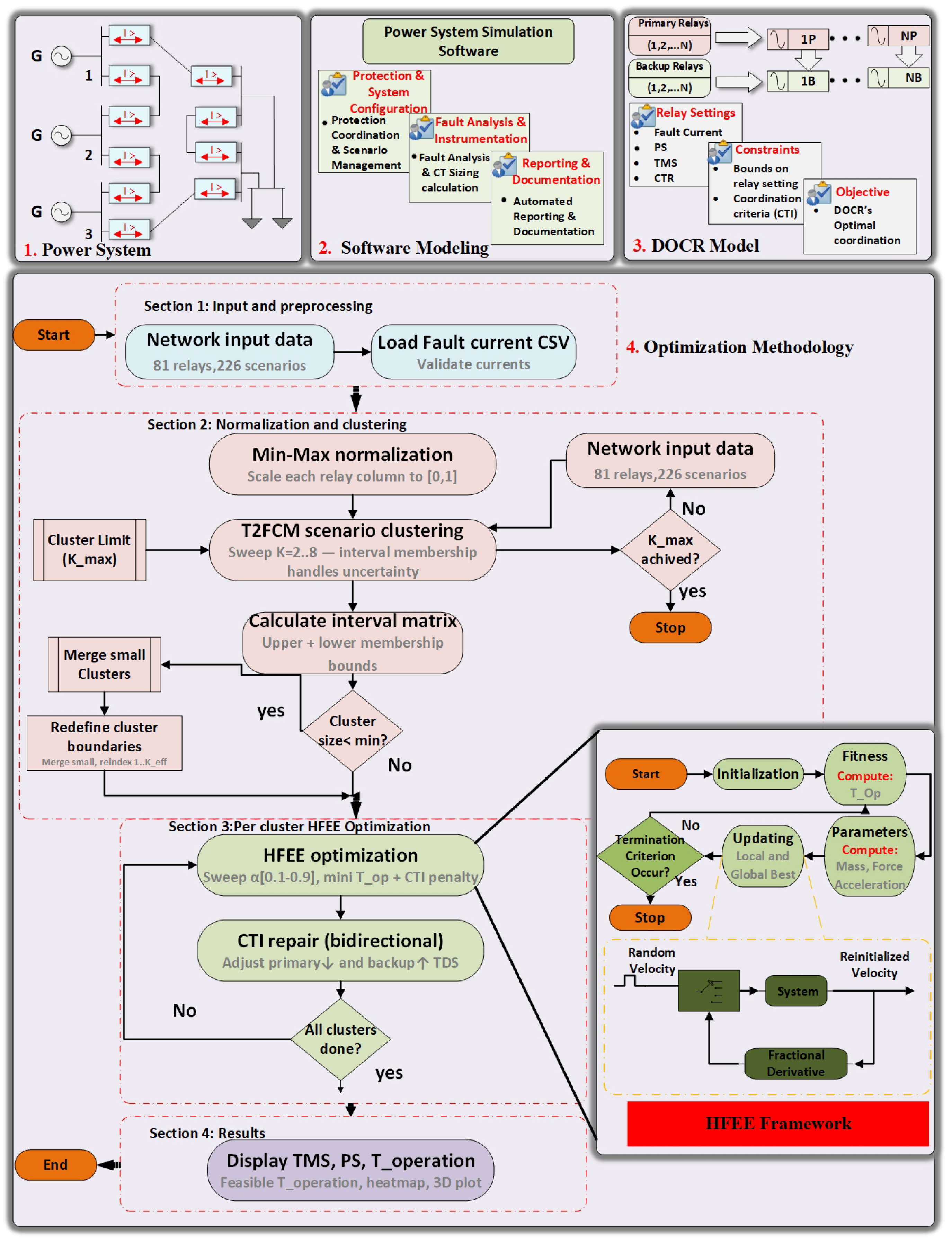
The proposed framework adopts a two-level hierarchical optimisation architecture. A zero-miscoordination criterion is applied: any ( K , α ) configuration producing CTI violations is excluded from the final ranking, ensuring that only strictly feasible solutions are reported [18]. The overall methodology, of HFEE framework, is illustrated in Figure 1.

4.2.1. Input Data Representation

The input to the clustering stage is the fault-current matrix X R 226 × 81 , where each row represents one fault scenario as an 81-dimensional feature vector of RMS short-circuit currents. The matrix structure is
X = 11936 0 0 0 11936 0 0 0 0 0 0 1972
where X i , j is the RMS three-phase short-circuit current (A) seen by relay j during scenario i, computed at 1% of line length from each bus per IEC 60255 [30].

4.2.2. Standard FCM Foundation

Standard FCM [27] assigns each scenario a soft membership u i j [ 0 , 1 ] subject to j = 1 K u i j = 1 , minimising
J m = i = 1 n j = 1 K u i j m x i v j 2
where m > 1 is the fuzzification parameter.

4.2.3. T2FCM Extension

T2FCM [19] replaces the scalar u i j with an interval [ u ̲ i j , u ¯ i j ] :
u ¯ i j = 1 l = 1 K x i v j x i v l 2 / ( m 1 1 )
u ̲ i j = 1 l = 1 K x i v j x i v l 2 / ( m 2 1 )
with fuzzification exponents m 1 = 2 and m 2 = 3 . The type-reduced membership for centroid computation is
u i j * = u ̲ i j + u ¯ i j 2
and updated as:
v j = i = 1 n ( u i j * ) m x i i = 1 n ( u i j * ) m
The algorithm iterates until the maximum membership change falls below 10 5 or 100 iterations are reached.

4.2.4. Setting Recombination and Deployment

A key distinction from the monolithic baseline is the per-cluster setting structure. T2FCM partitions the 226 fault scenarios into K = 6 disjoint groups; HFEE is then applied independently to each group, producing K = 6 complete sets of 81 TMS and 81 PS values—one set per cluster. Consequently, each relay stores K = 6 (TMS, PS) pairs in its non-volatile memory, one for each cluster. At runtime, the relay independently selects the active pair based on its local fault-current measurement, comparing the measured current against the per-cluster pickup thresholds precomputed offline from the cluster centroids. No inter-relay communication is required: each relay selects its setting group autonomously from a local decision rule, without exchanging data with any other relay. This is consistent with the multi-group capability of commercial numeric relays; the MiCOM P127 supports up to eight pre-loaded setting groups switchable via programmable binary inputs or local logic [32]. In contrast, the monolithic HFEE produces only a single (TMS, PS) pair per relay, requiring no group selection at all.

4.2.5. Cluster Count Restriction Range

The cluster count is swept from K = 2 to K = 8 . Below K = 6 , per-cluster scenario subsets are too large for the optimiser to reliably resolve all conflicting CTI constraints within the 100-iteration budget. Above K = 6 , wall-clock computation time increases proportionally, and the risk of splitting operationally coupled relay pairs across cluster boundaries rises, leading to CTI violations at K = 8 for α { 0.1 , 0.9 } . This behaviour is also discussed in Section 6, where the computation time– T op trade-off shows diminishing returns beyond K = 6 . Furthermore, the MiCOM P127 supports a maximum of eight setting groups [32]; K > 8 would exceed deployable hardware capacity. Detailed results for all ( K , α ) combinations are available at  https://github.com/Mubashar-3001/fpsogsa-ee-cluster (accessed on 10 May 2026). To complement the operational justification presented above, three established clustering validation indices were computed on the fault-current matrix X for K { 2 , , 8 } using the hard cluster assignments derived from K-means (as a proxy for the T2FCM hard labels, following standard practice in fuzzy clustering evaluation [33]). Table 2 reports the Silhouette index (higher is better), Davies–Bouldin index (lower is better), and Xie–Beni index (lower is better).
All three indices unanimously identify K = 4 as the statistically optimal cluster count for the fault-current data, exhibiting the highest Silhouette score (0.3115), the lowest Davies–Bouldin index (1.5460), and the lowest Xie–Beni index (1.2458). The operational parameter sweep (Section 6.3), however, identifies K = 6 as the configuration that minimises T op with zero CTI violations. This discrepancy is physically meaningful and expected: K = 4 produces the most internally cohesive clusters with the sharpest inter-cluster separation, but the coarser decomposition leaves each subproblem with a larger number of conflicting coordination constraints, making it harder for HFEE to find a feasible solution within the 100-iteration budget. K = 6 achieves finer decomposition, reducing per-cluster constraint complexity at the cost of some cluster purity, and enables HFEE to converge reliably to zero-violation solutions.
A second important observation from Table 2 is that all Silhouette values are below 0.35, indicating that the fault-current scenarios do not form sharply separated natural clusters. This is physically consistent with the meshed network topology of the IEEE 30-bus system, where similar fault-current magnitudes appear across multiple protection zones. Crucially, this finding provides the strongest validation for the choice of T2FCM over K-means or standard FCM: when cluster boundaries are inherently ambiguous, crisp and type-1 fuzzy assignments are unreliable, and the interval-valued memberships of T2FCM are essential to capture the genuine uncertainty in scenario-cluster assignment [28,29].

4.3. Hybrid Fractional Entropy Evolution (HFEE) Optimizer

The HFEE framework integrates fractional calculus and Shannon entropy into the PSO–GSA optimisation scheme [20]. Fractional calculus was first incorporated into PSO–GSA in [22]; Shannon entropy integration (without fractional calculus) was later introduced in [21].

4.3.1. Fractional-Order Velocity Update

Incorporating the Grünwald–Letnikov fractional derivative of order α introduces memory effects into the velocity update [34,35]:
v i n + 1 = α v i n + 1 2 α ( 1 α ) v i n 1 + 1 6 α ( 1 α ) ( 2 α ) v i n 2 + 1 24 α ( 1 α ) ( 2 α ) ( 3 α ) v i n 3 + c 1 r 1 · a c i ( t ) + c 2 r 2 · ( G best X i ( t ) )
where a c i ( t ) is the gravitational acceleration from GSA [10]. When α = 1 , Equation (14) reduces to standard PSO–GSA [36]. Lower values of α reduce the memory effect, encouraging broader exploration.

4.3.2. Shannon Entropy Integration

The swarm-diversity entropy H D ( X ) is computed at each iteration:
p i = d i j = 1 n d j , H D ( X ) = i = 1 n p i log p i
where d i is the Euclidean distance from particle i to G best . H D ( X ) modulates the velocity update:
v i ( t + 1 ) = ω v i ( t ) + c 1 r 1 1 + H D ( X ) a c i ( t ) + c 2 r 2 G best X i ( t )
When H D ( X ) falls below threshold H min , the worst-performing 20% of agents are reinitialised to restore diversity and prevent premature convergence.

4.4. Clustering-Decomposed HFEE Procedure

The complete procedure is summarised in Algorithm 1. Figure 1 illustrates the corresponding framework.
Algorithm 1: T2FCM Clustering-Decomposed HFEE for DOCR Coordination
Input: Fault-current matrix ( 226 × 81 ) , CTR, relay pairs, TMS/PS bounds, CTI = 0.3 s
Output: Optimised TMS and PS per relay; total T op ; CTI violations
Step 1: Data Preparation
1:Load fault currents; standardise to zero mean, unit variance
Step 2: T2FCM Clustering (Upper Level)
3:for each K { 2 , 3 , , 8 }  do
4:   Apply T2FCM with m 1 = 2 , m 2 = 3
5:   Compute interval memberships [ u ̲ i j , u ¯ i j ]
6:   Assign scenarios to clusters via u i j *
7:   Merge clusters with fewer than 3 scenarios
8:end for
Step 3: Per-Cluster HFEE Optimisation (Lower Level) [20]
9:for each α { 0.1 , 0.2 , , 0.9 }  do
10:   for each cluster C j  do
11:      Initialise 50 agents within TMS/PS bounds
12:      for iteration = 1 to 100 do
13:         Evaluate fitness (Equation (6))
14:         Compute gravitational mass, force, acceleration
15:         Compute H D ( X ) (Equation (15))
16:         Update velocity (Equations (14) and (16))
17:         Update positions; enforce bounds
18:         Update local and global best
19:         if  H D ( X ) < H min : reinitialise worst 20% of agents
20:      end for
21:   end for
22:end for
Step 4: Aggregation and Validation
23:Combine per-cluster solutions into the full 81-relay setting vectors
24:Evaluate system-wide T op and CTI compliance
25:Record T op , violations, entropy, per-relay times
26:Identify the best feasible ( K , α ) configuration

5. Test System and Experimental Setup

5.1. IEEE 30-Bus Extended Network

The extended IEEE 30-bus network is a sub-transmission/ distribution system consisting of 2 generators, 4 synchronous condensers, 13 lines at 132 kV, 4 transformers (132/33 kV), and 23 lines at 33 kV [4,37]. The complete system is protected by 81 DOCRs with 226 primary–backup coordination pairs. The single-line diagram, relay locations, and inter-relay coordination links are presented in [4].The corresponding CTRs are provided in Table 3, and the fault currents are in Table 4. The relay pairs and three-phase near-end RMS fault currents follow the IEC 60255 standard, as detailed in [4,5].

5.2. Current Transformer Ratio

The CTR directly affects optimisation outcomes because it determines the discrete pickup current values and consequently shifts the relay operating-time curve. The pickup current I p = CTR × PS appears in the PSM ratio I f / I p ; any change in CTR therefore alters relay sensitivity and operating time. Accurate CTR values from relay specifications are essential for producing implementable settings [4,6].
The CTRs used follow [4] and are summarised in Table 3. Three CT groups are applied: line relays (R1–R70) use a 1000/5 A ratio; transformer primary relays use 500/5 A; and transformer secondary relays use 2000/5 A. The pickup-current step size on the primary side is Δ I p = 0.01 × 5 × CTR = 0.05 × CTR [4]. This discrete quantisation is enforced throughout optimisation to ensure that all optimised PS values correspond to physically realisable tap positions on commercial relays, preventing miscoordination caused by impractical inter-tap settings.

5.3. Scenario Configuration and Excluded Pairs

Network topology changes are considered when determining pickup currents to prevent false tripping under transformer outage conditions. Five scenarios are evaluated: (1) all transformers in service, and (2)–(5) each of the four transformers individually out of service. For each scenario, the maximum load current across all conditions determines the pickup current for each relay. After verification, 226 valid fault scenarios are obtained.
Seven primary/backup pairs in the extended IEEE 30-bus system are structurally constrained such that no TMS or PS assignment can satisfy CTI  0.2  s, owing to the physical fault-current distribution. These pairs fall into two categories. Bidirectional pairs (R2→R3, R4→R1, R32→R33, R76→R77) arise from the meshed topology, where the same relay alternates between primary and backup roles depending on fault location. The directional element of the DOCR resolves this in practice by blocking operation for reverse-direction faults, ensuring the conflicting CTI constraints never apply simultaneously. Transformer backup pairs (R15→R74, R75→R79, R78→R75) involve transformer-connected relays where the fault-current distribution inherently favours the backup relay. These are addressed through dedicated current-differential protection, which provides faster and more selective operation than overcurrent time-grading [38]. Accordingly, these seven pairs are excluded from the CTI coordination metric, leaving 219 active coordination pairs, consistent with standard protection engineering practice [39].

5.4. Relay Pairs and Fault Currents

Table 4 presents a representative subset of the 226 primary–backup relay pairs and their three-phase near-end RMS fault currents. The matrix X , used as input to the clustering stage, is structured as in Equation (8), where X i , j is the RMS three-phase short-circuit current (A) seen by relay j during scenario i.
Table 4. IEEE  30-bus extended system relay pairs and fault currents [4,40].
No.Pri.Bkp. I f P I f B No.Pri.Bkp. I f P I f B No.Pri.Bkp. I f P I f B
1R1R411,936139977R23R2277951602153R46R5228802880
2R1R611,936105278R23R7677951181154R47R3985095472
3R2R37857209079R23R787795309155R47R4385091402
4R2R87857110080R23R79779510,345156R47R4685091654
5R2R107857110481R24R2513031049157R48R6028252825
6R2R127857117882R24R8113031021158R49R4148254825
7R3R211,936139983R25R2156603545159R50R2775177517
8R3R611,936105284R26R2336473396160R51R4538453845
9R4R17857209085R26R8136471008161R52R5439703970
10R4R87857110086R27R3012,3111166162R53R5128082808
11R4R107857110487R27R3212,311655163R54R2948634863
12R4R127857117888R27R3412,311655164R55R3110,4075203
13R5R212,156140389R27R3612,311369165R55R3310,4075203
14R5R412,156140390R27R7512,311748166R56R3542262225
15R6R143757375791R27R7712,311876167R56R5842262028
16R7R18737207892R27R7912,3119287168R57R3510,0642212
17R7R38737207893R28R4927992799169R57R5510,0647851
18R7R108737108594R29R2813,0532005170R58R5937502123
19R7R128737114895R29R3213,053647171R58R6237501628
20R8R135764160896R29R3413,053647172R59R4740124012
21R8R165764329797R29R3613,053365173R60R5760364419
22R8R73576418498R29R7513,053741174R60R6260361620
23R8R74576410,00999R29R7713,053868175R61R5765144407
24R9R187142073100R29R7913,0539202176R61R5965142107
25R9R387142073101R30R5323982398177R62R6427542754
26R9R887141078102R31R2813,6662036178R63R6127492749
27R9R1287141152103R31R3013,6661171179R64R8042191055
28R10R1836551529104R31R3413,666597180R65R6359871944
29R11R186612079105R31R3613,666358181R65R68598717
30R11R386612079106R31R7513,666750182R65R8059871045
31R11R8866110,711107R31R7713,666879183R66R70836836
32R11R1086611082108R31R7913,6669313184R67R6359421932
33R12R1565852454109R32R3377845157185R67R66594224
34R12R2065851150110R32R5677842651186R67R8059421039
35R12R2265851590111R33R2813,6662036187R68R6911021102
36R12R246585340112R33R3013,6661171188R69R6521242124
37R12R7665851165113R33R3213,666597189R70R6715891589
38R12R786585301114R33R3613,666358190R71R6154152725
39R12R79658510,185115R33R7513,666750191R71R6454152736
40R13R520852085116R33R7713,666879192R72R765571532
41R14R757611524117R33R7913,6669313193R72R1365571648
42R14R1657613364118R34R3177845157194R72R1665573379
43R14R735761190119R34R5677842651195R73R384232459
44R14R74576110,178120R35R2813,7932018196R73R4042321793
45R15R740371525121R35R3013,7931161197R73R4242321993
46R15R1340371642122R35R3213,793602198R75R1179351467
47R15R734037180123R35R3413,793602199R75R1579352529
48R15R74403710,205124R35R7513,793744200R75R2079351184
49R16R1156721457125R35R7713,793872201R75R2279351630
50R16R2056721178126R35R7913,7939234202R75R247935348
51R16R2256721623127R36R5597737803203R75R787935307
52R16R245672346128R36R5897732012204R75R79793510,438
53R16R7656721186129R37R4014,0201712205R76R2811,4172041
54R16R785672312130R37R4214,0201951206R76R3011,4171175
55R16R79567210,398131R37R7214,0201342207R76R3211,417660
56R17R938381684132R37R7414,02015,205208R76R3411,417660
57R18R1929892989133R38R4431013101209R76R3611,417372
58R19R1169651448134R39R3812,873432210R76R7711,417881
59R19R1569652498135R39R4212,8731968211R76R7911,4179334
60R19R22696511,611136R39R7212,8731356212R77R1174451467
61R19R246965344137R39R7412,87315,366213R77R1574452529
62R19R7669641181138R40R4347741400214R77R2074451184
63R19R786965303139R40R4647741666215R77R2274451630
64R19R79696510,316140R40R4847741712216R77R247445348
65R20R1718211821141R41R3812,607450217R77R7674451194
66R21R1165631459142R41R4012,6071758218R78R2878312042
67R21R1565632516143R41R7212,6071349219R78R3078311175
68R21R2065631177144R41R7412,60715,297220R78R327831660
69R21R246563337145R42R5038823882221R78R347831660
70R21R7665631188146R43R3739443944222R78R367831372
71R21R786563306147R44R3987855443223R78R7578313010
72R21R79656310,383148R44R4687851654224R80R2345123459
73R22R262777607149R44R4887851700225R80R2545121053
74R23R1177951453150R45R3985425467226R81R6319721972
75R23R1577952505151R45R4385421400
76R23R2077951173152R45R4885421698

5.5. Algorithm Control Parameters

Table 5 summarises the control parameters used by the HFEE optimiser across all experiments. The TMS and PS bounds follow the MiCOM P127 specifications [32], ensuring that all optimised settings are directly deployable on commercial relays. The population size of 50 particles balances exploration capability and computational cost for the 162-dimensional search space. A total of 100 iterations per run and 50 independent runs per configuration ensures statistical reliability. The sweep over nine fractional orders and seven cluster counts yields 63 distinct clustered configurations, amounting to 63 × 50 = 3150 optimisation runs.
All experiments were conducted in MATLAB R2018a on a system equipped with an Intel Core i7 processor (2.00 GHz) and 8 GB RAM. Wall-clock computation time was measured using MATLAB’s tic/toc facility averaged over 50 independent runs at the best configuration ( K = 6 , α = 0.1 ) to obtain a reliable timing estimate. Reported computation times are wall-clock seconds and therefore reflect practical deployment cost rather than theoretical CPU-cycle counts.

6. Results and Discussion

6.1. Statistical Robustness and Sensitivity Analysis

To assess the reliability of both the clustered and non-clustered configurations, 50 independent runs were executed for each method.
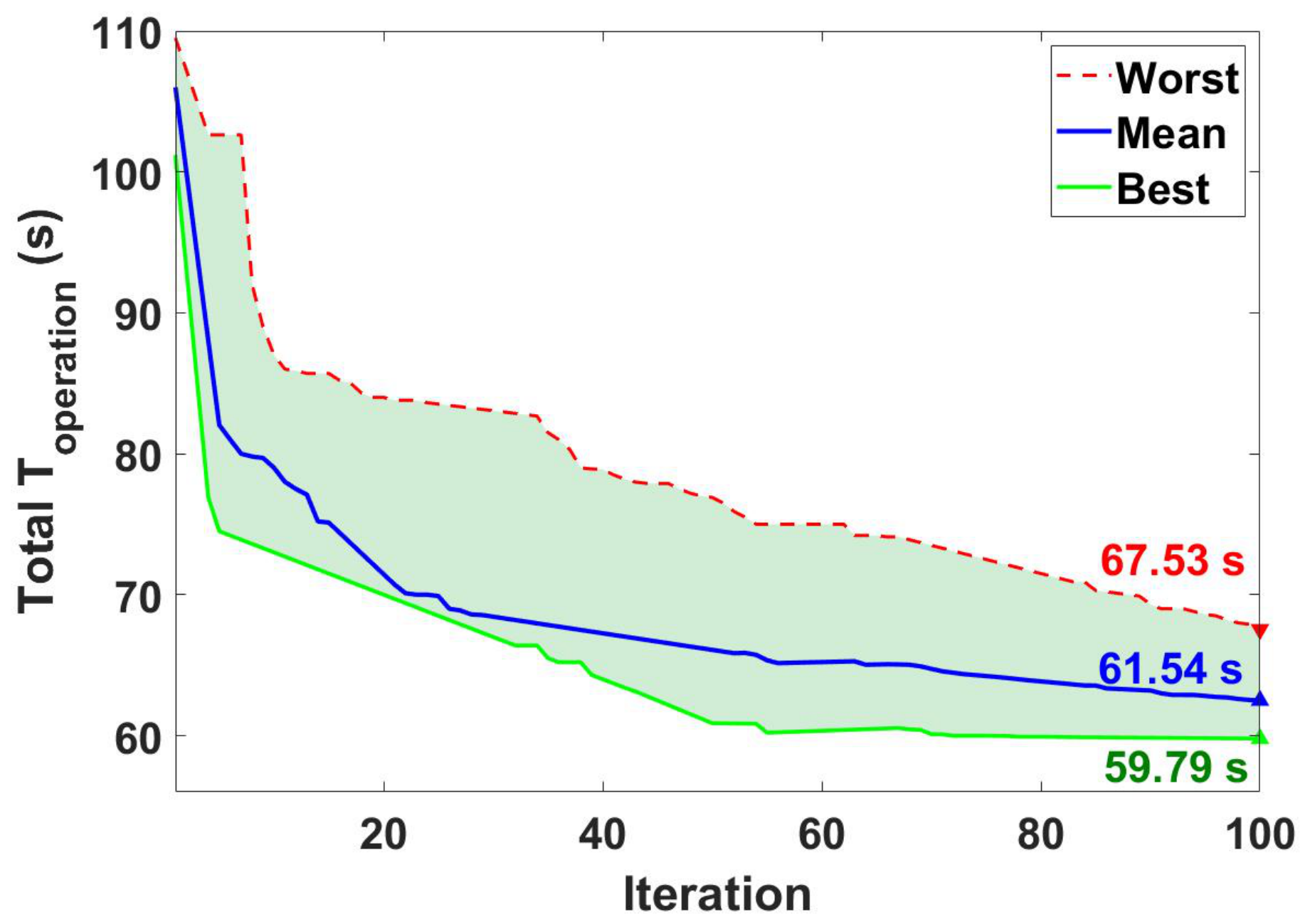
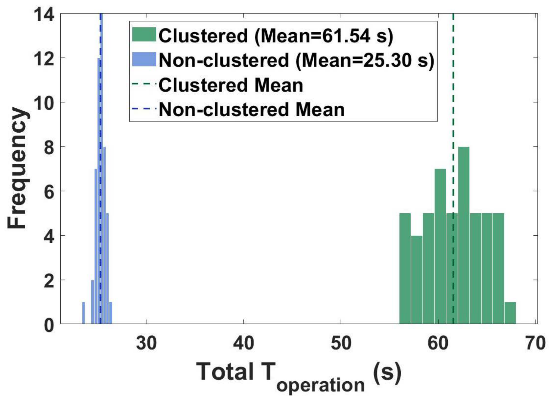
For the proposed T2FCM+HFEE framework ( K = 6 , α = 0.1 ), T op ranged from a best of 59.79 s to a worst of 67.53 s, with a mean of 61.54 s, standard deviation of 3.04 s, coefficient of variation (CV) = ( 3.04 / 61.54 ) × 100 = 4.94 % , and 95% confidence interval (CI) = 61.54 ± 0.84 s (i.e., [ 60.70 , 62.38 ] s, computed as x ¯ ± 1.96 σ / 50 ).
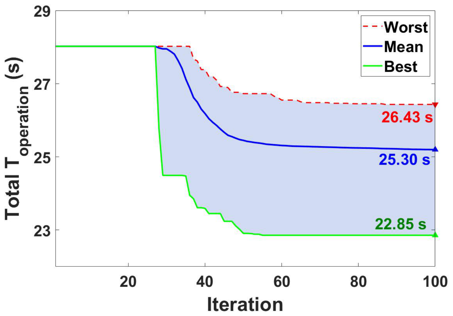
For the non-clustered HFEE baseline, the best result across all α values was 22.85 s at α = 0.7 , with a mean of 25.30 s, worst of 26.43 s, standard deviation of 0.51 s, CV = ( 0.51 / 25.30 ) × 100 = 2.02 % , and 95% CI = 25.30 ± 0.14 s ( [ 25.16 , 25.44 ] s). The substantially lower CV of the non-clustered variant (2.02% vs. 4.94%) reflects the simpler, single-level search landscape; however, this consistency comes at the cost of ignoring inter-scenario diversity and producing a single relay-setting vector that is not optimised across heterogeneous fault conditions.
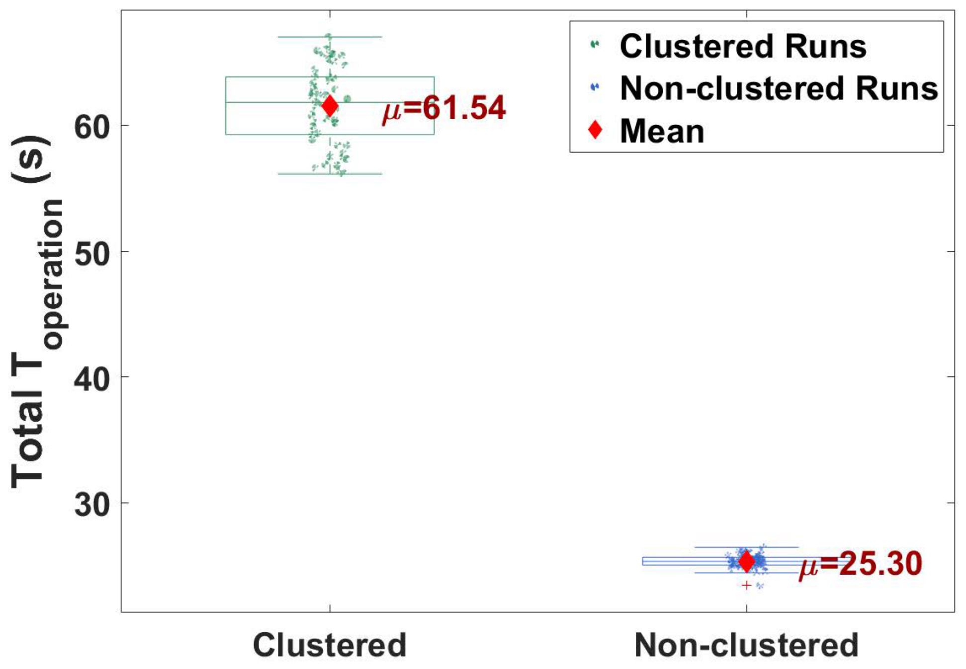
A Wilcoxon signed-rank test and a Wilcoxon rank-sum test were applied to the two 50-run distributions; both returned p < 0.0001 , confirming that the difference in T op between the clustered and non-clustered approaches is statistically significant at the 1% level. The convergence behaviour across the best, mean, and worst runs for both methods is illustrated in Figure 2 and Figure 3, and the complete 50-run distributions are compared in the box plot of Figure 4 and the frequency distribution of Figure 5. The shaded area between the maximum and minimum values indicates the bandwidth, and all solutions lie within it.

6.2. Ablation Study: Clustered vs. Non-Clustered HFEE

The ablation study isolates the contribution of the T2FCM decomposition stage by comparing two configurations on the same extended IEEE 30-bus system (81 relays, 226 pairs): monolithic HFEE (no clustering) and T2FCM+HFEE.
Operational performance: Monolithic HFEE achieves a mean T op of 25.30 s, representing a 29.19% improvement over the prior best result of 35.73 s reported in [4]. T2FCM+HFEE achieves a mean T op of 61.54 s, which is higher in absolute terms. This increase arises because the clustering decomposition optimises each cluster of scenarios independently: within each cluster, HFEE minimises the operating time for that cluster’s scenario subset rather than all 226 scenarios simultaneously, and the CTI threshold is set to the stricter 0.3 s (versus 0.2 s for the baseline). The total T op is the sum of per-cluster optimal values, which is inevitably higher than the monolithic optimum.
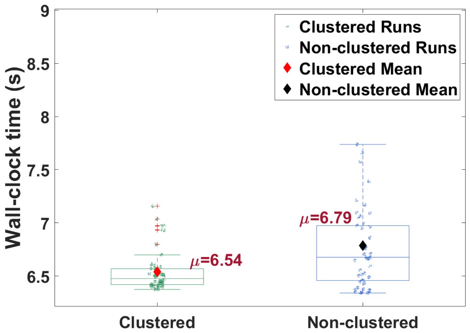
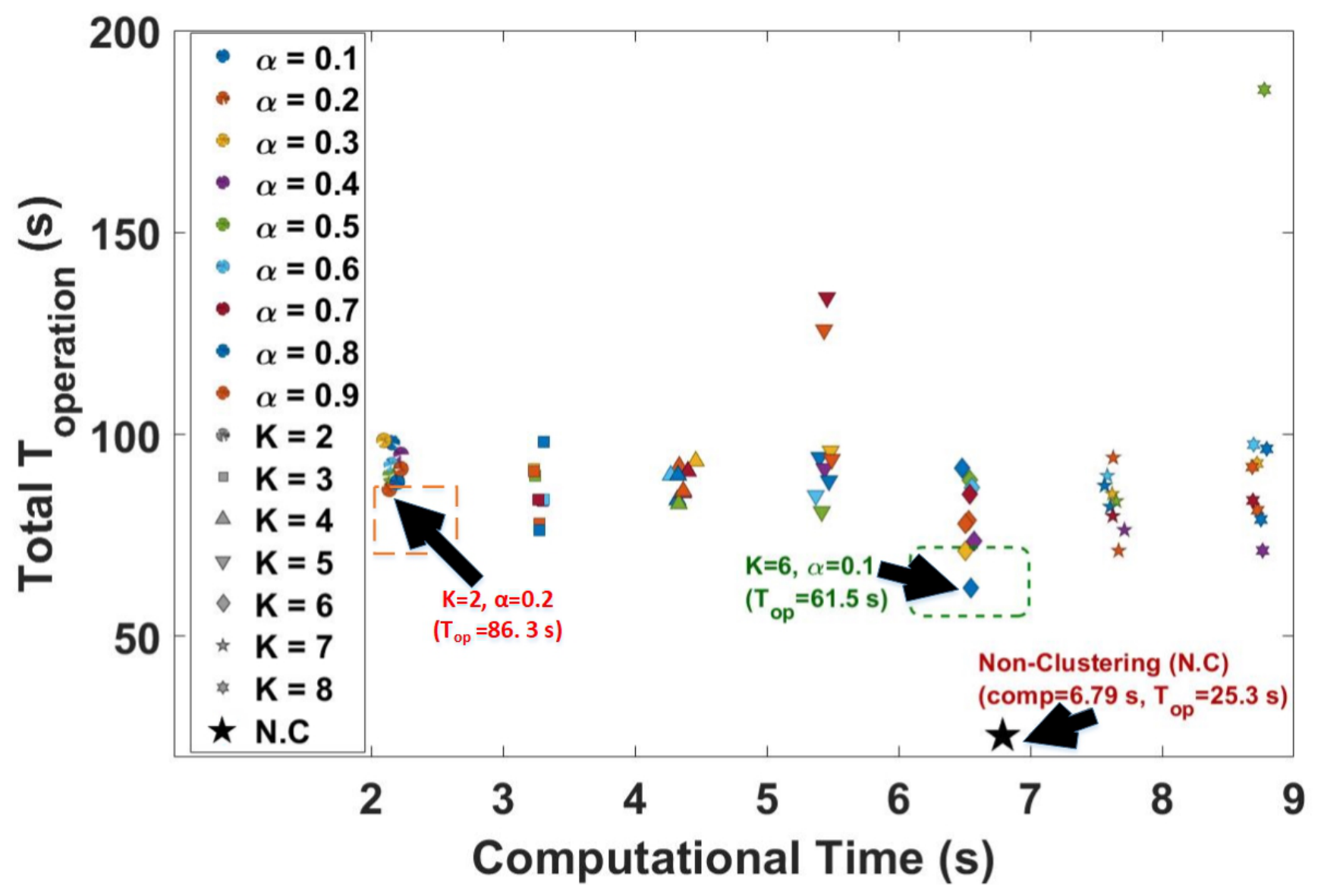
Computational performance: Wall-clock computation time at K = 6 , α = 0.1 is 6.54 ± 0.19 s (mean ± std, N = 50 ), compared to 6.79 s for monolithic HFEE—a 3.68% reduction. For K = 2 , the computation time is 2.18 s, representing a 66.67% reduction relative to the K = 6 reference point and a 67.9% reduction relative to the non-clustered baseline. The computational complexity is analysed in Section 6.5.
Practical advantages of clustering: Although the clustered formulation does not achieve the lowest absolute T op , it offers four practical advantages over the monolithic approach: decomposition scalability (the problem splits into K independent subproblems of 162 / K variables each); parallel computation (K clusters solved concurrently, offering a theoretical K-fold speedup); multi-scenario robustness (226 simultaneous fault scenarios versus a single scenario per pair in [4]); and modular re-optimisation (only affected clusters need updating under network modifications).
Table 6 presents the ablation comparison. The proposed standalone HFEE achieves a mean T op of 25.30 s, representing a 29.19% improvement over the prior best result of HEPSO/TFWO (35.73 s [4]) at the same CTI level of 0.20 s. This confirms that HFEE, applied monolithically without any decomposition, establishes a new state-of-the-art baseline for the extended IEEE 30-bus benchmark. The T2FCM+HFEE configuration (CTI = 0.30 s, K = 6, α = 0.1 ) achieves 61.54 s with zero violations under the stricter coordination margin, with a 3.68% reduction in wall-clock computation time and full multi-scenario robustness across 226 simultaneous fault scenarios. K-means+HFEE and FCM+HFEE were excluded from this comparison as preliminary evaluations showed consistent CTI violations on the 226-constraint system, indicating that crisp and type-1 fuzzy partitioning cannot reliably decompose the coordination problem at this scale; this finding further validates the choice of T2FCM as the clustering stage.

6.3. T2FCM Parameter Sweep and Heatmap Analysis

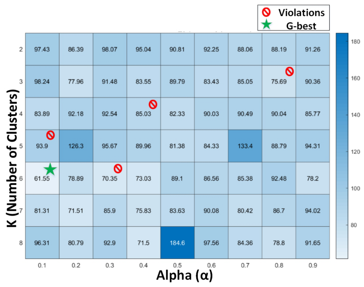
Figure 6 presents the heatmap of T op across all 63 ( K , α ) configurations. Each cell reports the mean T op from 50 independent runs; configurations producing CTI violations are marked with a prohibited symbol. The global feasible minimum is T op = 61.54 s at K = 6 , α = 0.1 .
Two principal trends are evident. First, α = 0.1 consistently yields the best results across most cluster counts. This indicates that reduced velocity memory promotes broader search-space exploration, which is consistent with the nature of the decomposed subproblems, where each cluster requires the independent discovery of a local optimum in a distinct region of the setting space. Second, T op is non-monotonic in K: performance improves from K = 2 towards K = 6 as finer decomposition reduces per-cluster coordination conflict, then degrades for K > 6 as clusters become too small to span coherent protection zones; wall-clock computation time rises proportionally throughout (Section 6.5).
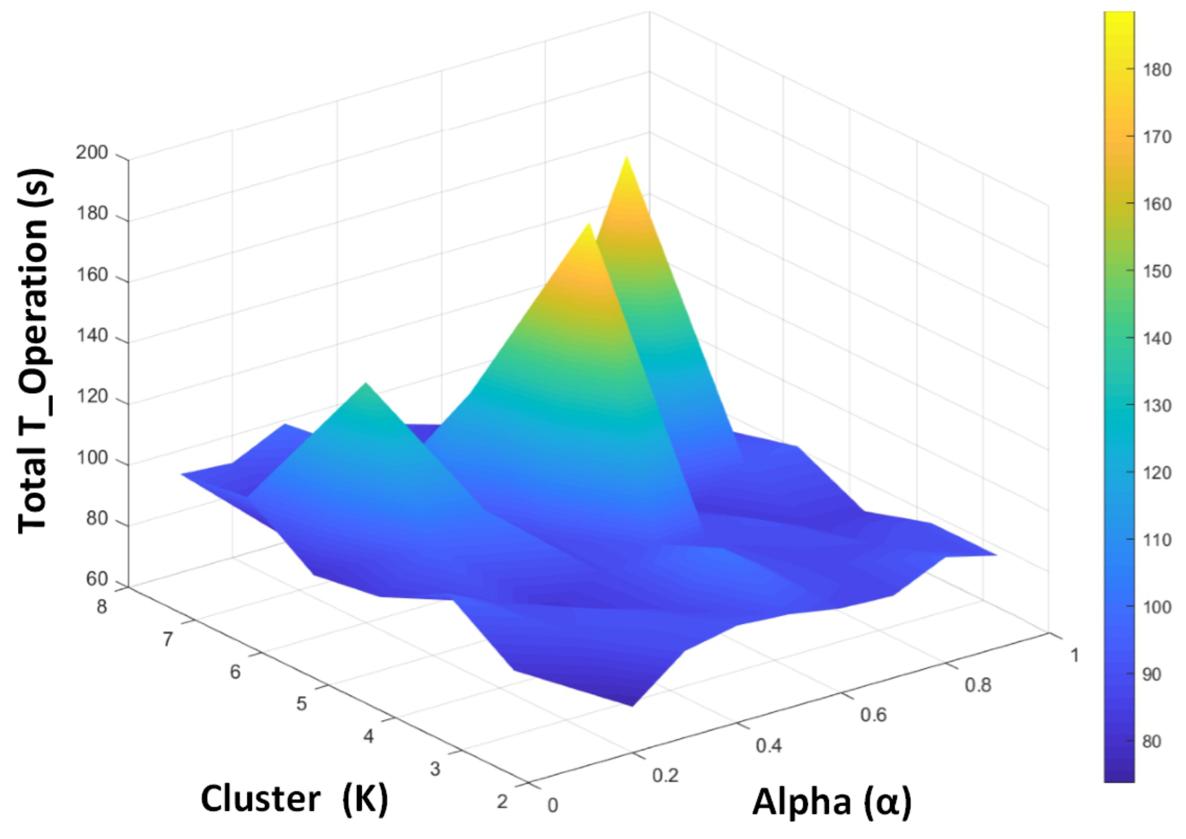
For a full visualisation of all 3150 solutions, the 3D surface plot in Appendix (Figure A1) shows the α K T op landscape; the majority of results cluster near the lower operational-time boundary, confirming the robustness of the proposed method.

6.4. Cluster Decomposition for the Best Configuration ( K = 6 , α = 0.1 )

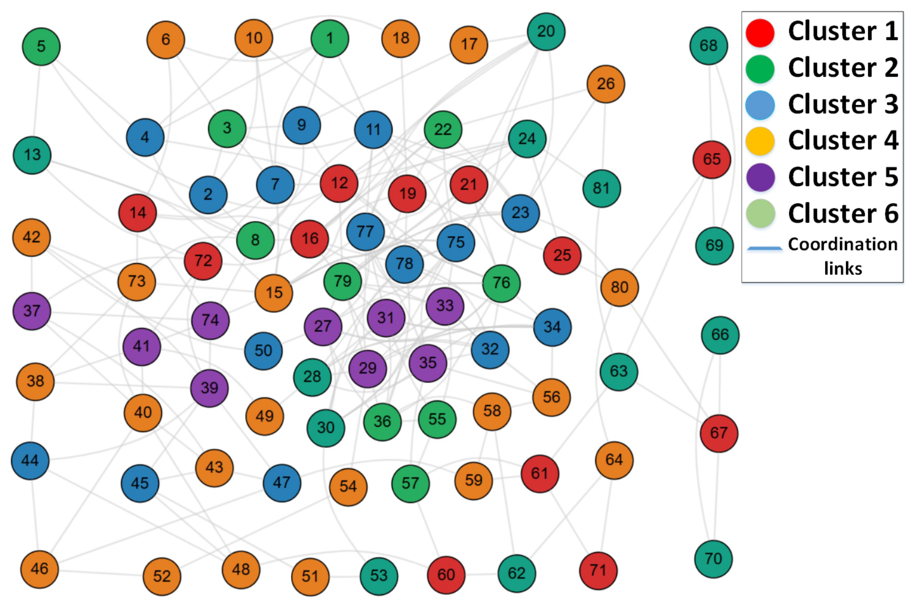
Table 7 summarises the relay-to-cluster assignment for the best configuration. The 81 relays are partitioned into six groups, each with its own TMS and PS values.
Cluster 4 has the highest relay count (22) and per-cluster T op (15.23 s), corresponding to distribution-level relays in the 33 kV section where meshed topology creates complex coordination requirements. Cluster 6 has the lowest per-cluster T op (0.85 s), comprising transformer-adjacent relays operating under simpler coordination constraints. The entropy range (0.811–3.573) indicates some variation in relay load distribution across clusters; this is expected given the heterogeneous nature of the six protection zones. The relay clusters are also shown in Figure 7, where different colours indicate distinct cluster groupings.
Approximately 15–20% of the 226 scenarios lie near protection-zone boundaries. Crisp clustering methods force these scenarios into a single cluster, potentially splitting operationally coupled relay pairs across cluster boundaries and causing CTI violations. T2FCM’s interval-valued memberships allow such scenarios to maintain partial participation in adjacent clusters, preserving coordination chain integrity. The FOU width furthermore serves as a quantitative confidence indicator: wide intervals flag scenarios where accurate coordination is most critical.

PhysicalInterpretation of Relay Settings at Boundary Values

The 81 relays are partitioned into six groups, each with its own TMS and PS values, reveals that several relays converge to boundary values of the decision space, specifically PS = 0.5 (minimum) or PS = 2.5 (maximum), and TMS = 0.10 (minimum) or TMS = 1.00 (maximum). These settings are physically meaningful rather than indicative of optimiser failure, for two reasons. First, relays assigned PS = 0.5 and TMS = 0.10 are configured for maximum sensitivity and minimum time delay; this is appropriate for relays positioned close to the fault source, where rapid isolation is critical and the risk of false tripping is low due to the high PSM ratio. Second, relays assigned TMS = 1.00 (maximum delay) serve as remote backup protection for fault paths where primary relays already provide fast clearance; the large time delay ensures selectivity without requiring tight TMS precision. The fact that all 219 active relay pairs satisfy the 0.3 s CTI requirement with zero violations confirms that these boundary-value settings are coordination-compliant and reflect a genuine engineering optimum for their respective cluster subproblems. The assignment of boundary values to certain relays is further consistent with the discrete-variable treatment of PS [4], where the coarse tap-step resolution naturally drives solutions towards the nearest feasible boundary point when that point satisfies all constraints.

6.5. Computational Complexity and Wall-Clock Time

The total number of fitness evaluations for the monolithic non-clustered approach is
P × maxIt × n scen × n pairs = 50 × 100 × 226 × 226 = 255 , 380 , 000
For the clustered approach ( K = 6 ),
K × P × maxIt × ( n scen / K ) × n pairs = 6 × 50 × 100 × 38 × 226 = 257 , 640 , 000
Although the total evaluation counts are similar, each per-cluster evaluation call processes only n scen / K 38 scenarios rather than all 226, yielding a benchmark cost ratio of approximately 5.95 × cheaper per cluster call. Furthermore, the K = 6 clusters are fully independent and can be solved concurrently on K cores, offering a theoretical 6 × parallel speedup.
Table 8 reports estimated wall-clock computation times for all 63 ( K , α ) configurations, linearly scaled from the measured point K = 6 , α = 0.1 ( 6.54 ± 0.19 s, N = 50 ). Note that wall-clock time scales linearly with K because each additional cluster adds one independent HFEE run (each of the same 100-iteration budget); α does not affect computation time, so all columns are identical. A comparison of clustered and non-clustered wall-clock times is shown in Figure 8.
Table 8 also reveals an important trade-off: selecting K = 2 reduces computation time to 2.18 s, a 66.67% reduction relative to K = 6 and a 67.9% reduction relative to non-clustered HFEE.
However, at K = 2 and α = 0.2 , T op rises to 86.39 s—a significant penalty in operational performance. This trade-off is visualised in Figure 9, where each point represents one of the 63 configurations; the non-clustered result is marked with a star. Practitioners can use this figure to select an appropriate ( K , α ) pair based on their specific balance of operational and computational requirements.
Table 8 and Figure 9 together provide a practical decision guide for selecting ( K , α ) based on engineering priorities. If total operational time is the primary objective, K = 6 and α = 0.1 yield the best T op of 61.54 s, with a moderate wall-clock time of 6.54 ± 0.19 s. Conversely, if computational speed is the priority, K = 2 and α = 0.2 reduce wall-clock time to 2.18 ± 0.11 s at the cost of a higher T op of 86.39 s. For applications where neither objective is dominant, K = 3 and α = 0.2 offer an intermediate trade-off, achieving T op = 77.96 s with a wall-clock time of 3.27 ± 0.13 s. This flexibility allows protection engineers to select a configuration that best suits their specific operational and computational constraints, without re-running the full parameter sweep.

6.6. CTI Margin Validation

To verify coordination integrity for the best configuration ( K = 6 , α = 0.1 ), the CTI margin Δ p = T b , p T p , p was evaluated for all 219 active primary–backup pairs using the optimised relay settings. All 219 pairs satisfied the 0.3 s CTI requirement, with zero violations. Table 9 presents the TMS and PS values alongside the minimum CTI margin for selected relays. The symbol denotes pairs where the directional element resolves the coordination constraint, as described in Section 5.
The minimum observed CTI margin across all 219 active pairs is 0.200 s (R81), which satisfies the IEC 60255 minimum of 0.2 s [30] with no surplus; this relay is transformer-adjacent and its margin is constrained by the physical fault-current ratio. The maximum margin is 3.332 s (R80), reflecting the conservative settings assigned to line relays with low fault-current exposure. The relatively wide margin range (0.200–3.332 s) indicates that T2FCM clustering successfully preserves the coordination hierarchy across all active pairs, including those near protection-zone boundaries.

6.7. Comparison with State-of-the-Art Methods

The proposed T2FCM+HFEE method achieves a mean T op of 61.54 s with zero CTI violations on the 81-relay extended system with six groups have their corresponding TMS and PS values listed in Table 10. Compared with methods limited to the 38-relay configuration (fewer than 120 constraints), the proposed framework handles a problem that is 2.1 × larger in decision variables and 3.3 × more constrained, demonstrating scalability for large-scale protection systems. The SQP-based method of Birla et al. [7] achieved 116.50 s on only 38 relays; the proposed method achieves 61.54 s on 81 relays—a 47.2% reduction despite a significantly larger problem, and a 67% improvement over Al-Bhadely and Inan [25] on the same relay count.
A direct comparison between T2FCM+HFEE and HEPSO/TFWO is not straightforward, as the two methods operate under different problem formulations and objectives: HEPSO/TFWO targets absolute T op minimisation per pair, whereas the proposed clustering framework prioritises computational scalability and multi-scenario robustness, accepting a trade-off in absolute operational time. A valid comparison is possible between the non-clustered HFEE and HEPSO/TFWO under identical conditions (CTI = 0.2 s, 81 relays, 226 pairs): non-clustered HFEE achieves a mean T op of 25.30 s, representing a 29.19% improvement over HEPSO/TFWO at the same constraint level. Among clustering-based methods, Zand et al. [18] achieved 52.33 s on the 38-relay system using a Fmincon algorithm with K-means; the proposed approach addresses a significantly larger and more constrained problem (226 pairs vs. fewer than 120).
The entropy term H D ( X ) in the velocity update (Equation (16)) enhances both swarm exploration and coordination balance: the ( 1 + H D ( X ) ) factor amplifies the exploratory component when diversity is high, while a low H D ( X ) triggers reinitialisation, preventing premature convergence. Simultaneously, the relay-time entropy H ( X ) in the objective (Equation (6)) promotes uniform relay utilisation, consistent with [20,21].
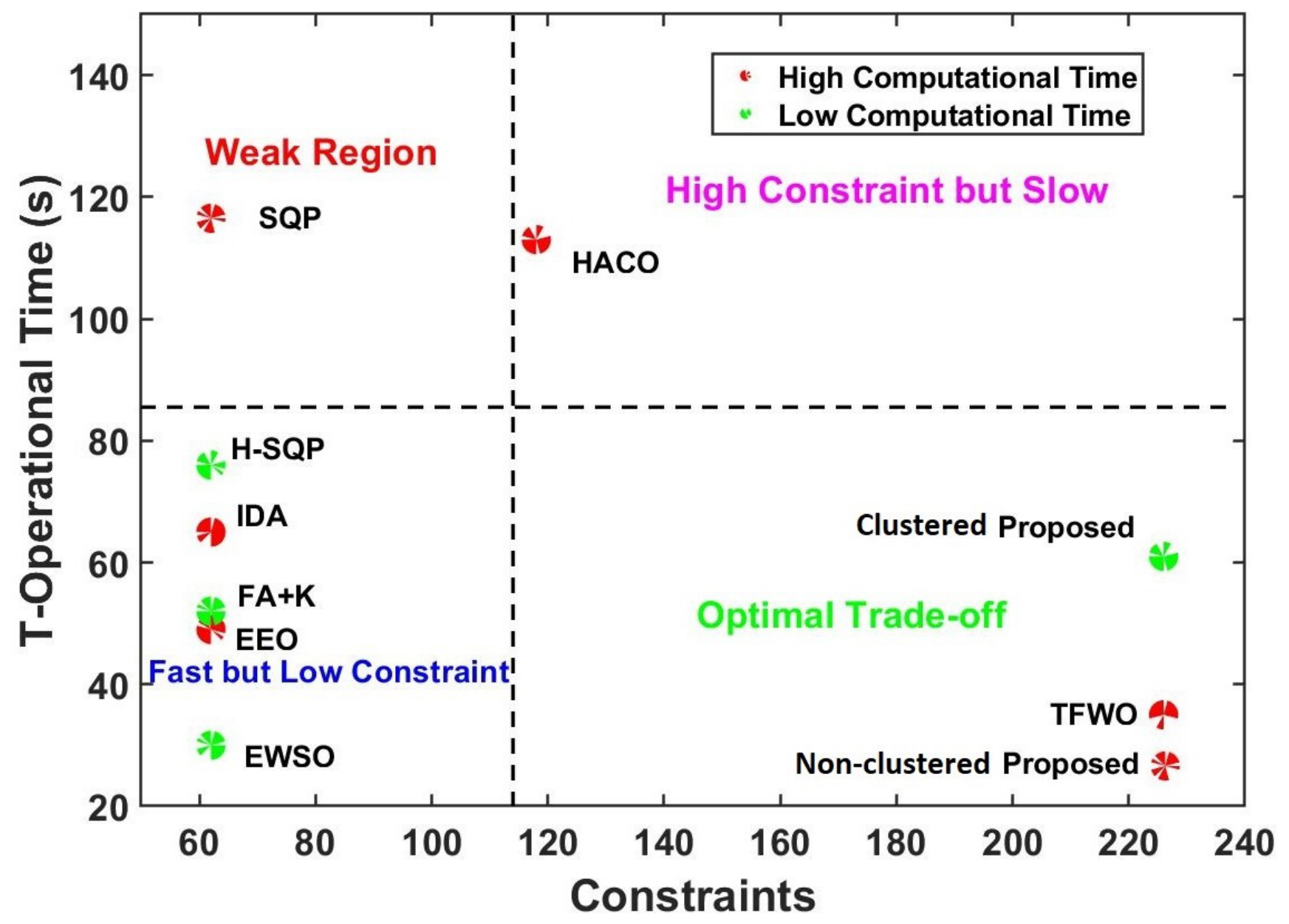
Figure 10 presents the 4-quadrant performance analysis. Methods in the top-left quadrant (e.g., SQP) exhibit high T op at low constraint counts—the weak region. Methods in the top-right quadrant (e.g., HACO) are constrained but operationally slow. Methods in the bottom-left quadrant (e.g., IDA, EEO, EWSO) achieve low T op but on low-constraint systems. The optimal trade-off region (bottom-right) captures methods that achieve low T op at high constraint counts; TFWO and both proposed methods (non-clustered HFEE and T2FCM+HFEE) fall in this region. Non-clustered HFEE achieves the lowest T op (25.30 s) at the highest constraint count (226), with high computational time; the clustered proposal achieves low computational time at the cost of higher T op , with the added benefits described in Section 4.2.4.

7. Conclusions

This study presented and validated both a standalone HFEE framework and a T2FCM clustering-decomposed HFEE framework for the coordination of directional overcurrent relays on the extended IEEE 30-bus system (81 relays, 226 primary—backup coordination pairs).
Standalone HFEE (monolithic, no clustering) achieves a 29.19% improvement over the reported best result of 35.73 s on the same system [4]—establishing a new state-of-the-art baseline for the extended IEEE 30-bus benchmark. T2FCM+HFEE achieves a mean T op of 61.54 s with zero CTI violations across all active relay pairs. The clustering decomposition reduces wall-clock computation time by 3.68–66.67% relative to the non-clustered baseline depending on K, at the cost of a higher absolute T op . The fractional order α = 0.1 consistently yields the best results, confirming that reduced velocity memory promotes effective exploration in the decomposed subproblems.
The two-level hierarchical architecture demonstrates scalability for simultaneous sub-transmission and distribution relay coordination, handling 162 decision variables and 226 constraints through six independently optimisable subproblems. The communicationless, entirely offline multi-group deployment strategy—compatible with the MiCOM P127 relay’s eight-group capability—requires no hardware upgrades or real-time communication links.
The primary limitations of this study are as follows: (1) the clustered T op is higher than monolithic methods, accepted in exchange for scalability and parallel decomposability; (2) the clustered framework requires each relay to store K distinct (PS, TMS) pairs—one per cluster—meaning a K = 6 configuration demands six independent setting groups per relay; this is compatible with the MiCOM P127’s eight-group capability [32] but may exceed the capacity of legacy relay hardware; (3) highly imbalanced clusters may reduce the theoretical K-fold parallel speedup.
Future work will extend the framework to dynamic fault scenarios, integrate distance relays alongside DOCRs, and explore multi-objective formulations balancing T op , computational cost, and protection reliability.

Author Contributions

Conceptualisation, M.J. and L.K.; methodology, M.J. and Y.M.; software, M.J.; validation, Y.M.; formal analysis, M.J.; investigation, M.J. and Y.M.; resources, L.K. and S.M.; data curation, M.J.; writing—original draft, M.J.; writing—review and editing, L.K. and S.M.; visualisation, M.J.; supervision, L.K. and Y.M.; project administration, L.K. and S.M.; funding acquisition, S.M. and M.S. All authors have read and agreed to the published version of the manuscript.

Funding

This research received no external funding.

Institutional Review Board Statement

Not applicable.

Informed Consent Statement

Not applicable.

Data Availability Statement

All data and code supporting this study are available at https://github.com/Mubashar-3001/fpsogsa-ee-cluster (accessed on 10 May 2026).

Conflicts of Interest

The authors declare no conflicts of interest.

Abbreviations

The following abbreviations are used in this manuscript:
ACOAnt colony optimisation
CTICoordination time interval
CTRCurrent transformer ratio
DOCRDirectional overcurrent relay
EEOEnhanced equilibrium optimiser
EWSOEnhanced water strider optimiser
FCMFuzzy C-Means (standard, type-1)
FOUFootprint of uncertainty
GSAGravitational search algorithm
H-ACOHybrid ant colony optimisation
HFEEHybrid Fractional Entropy Evolution
HEPSOHigh-exploration particle swarm optimisation
IDAInformative differential evolution algorithm
MILPMixed-integer linear programming
NINormal inverse (relay characteristic)
PSPlug setting
PSMPlug setting multiplier
PSOParticle swarm optimisation
SQPSequential quadratic programming
T2FCMType-2 Fuzzy C-Means
TFWOTurbulent flow of water-based optimisation
TMSTime multiplier setting
Nomenclature:
SymbolDescription
T op Total operational time (s)
T i Operating time of relay i (s)
TMS Time multiplier setting
I f Fault current (A)
α Fractional order
T b , T p Backup/primary relay operating time (s)
CTRCurrent transformer ratio
u i j FCM membership degree of scenario i in cluster j
m 1 , m 2 T2FCM fuzzification exponents
λ penalty CTI penalty weight
G best Global best position (HFEE)
r 1 , r 2 Uniform random numbers in [ 0 , 1 ]
FOUFootprint of uncertainty
H ( X ) Shannon entropy (diversity index)
H D ( X ) Swarm-diversity entropy (HFEE)
PS Plug setting
I p Pickup current (A)
KNumber of clusters
CTICoordination time interval (s)
PSMPlug setting multiplier
[ u ̲ i j , u ¯ i j ] T2FCM interval membership
v j Centroid of cluster j
λ H Entropy reward weight
a c i ( t ) Gravitational acceleration of agent i
nNumber of particles
SNumber of fault scenarios

Appendix A

Figure A1. 3D surface plot of all solutions: fractional order α versus cluster count K versus T op (s). The majority of solutions cluster near the lower operational-time boundary, confirming the robustness of the T2FCM+HFEE framework across the parameter space.
Energies 19 02943 g0a1

References

  1. Moravej, Z.; Adelnia, F.; Abbasi, F. Optimal coordination of directional overcurrent relays using NSGA-II. Electr. Power Syst. Res. 2015, 119, 228–236. [Google Scholar] [CrossRef] [Scilit]
  2. Adelnia, F.; Moravej, Z.; Farzinfar, M. A new formulation for coordination of directional overcurrent relays in interconnected networks. Int. Trans. Electr. Energy Syst. 2015, 25, 120–137. [Google Scholar] [CrossRef] [Scilit]
  3. Saleh, K.A.; Zeineldin, H.H.; Al-Hinai, A.; El-Saadany, E.F. Optimal coordination of directional overcurrent relays using a new time–current–voltage characteristic. IEEE Trans. Power Deliv. 2014, 30, 537–544. [Google Scholar] [CrossRef] [Scilit]
  4. Bayazidi, A.; Abdali, A.; Vasquez, J.C. Optimal coordination of directional overcurrent relays in power energy systems with emphasis on the discreteness of variables: Comprehensive comparisons. Heliyon 2024, 10, e37972. [Google Scholar] [CrossRef] [Scilit] [PubMed]
  5. Abdelaziz, A.Y.; Talaat, H.E.A.; Nosseir, A.I.; Hajjar, A.A. An adaptive protection scheme for optimal coordination of overcurrent relays. Electr. Power Syst. Res. 2002, 61, 1–9. [Google Scholar] [CrossRef] [Scilit]
  6. Foqha, T.; Alsadi, S.; Omari, O.; Refaat, S.S. Optimization techniques for directional overcurrent relay coordination: A comprehensive review. IEEE Access 2024, 12, 1952–2006. [Google Scholar] [CrossRef] [Scilit]
  7. Birla, D.; Maheshwari, R.P.; Gupta, H.O. A new nonlinear directional overcurrent relay coordination technique, and banes and boons of near-end faults based approach. IEEE Trans. Power Deliv. 2006, 21, 1176–1182. [Google Scholar] [CrossRef] [Scilit]
  8. Damchi, Y.; Dolatabadi, H.R.; Mashhadi, H.R.; Sadeh, J. MILP approach for optimal coordination of directional overcurrent relays in interconnected power systems. Electr. Power Syst. Res. 2018, 158, 267–274. [Google Scholar] [CrossRef] [Scilit]
  9. Rathinam, A.; Sattianadan, D.; Vijayakumar, K. Optimal coordination of directional overcurrent relays using particle swarm optimization technique. Int. J. Comput. Appl. 2010, 1, 93–97. [Google Scholar] [CrossRef] [Scilit]
  10. Rashedi, E.; Nezamabadi-pour, H.; Saryazdi, S. GSA: A gravitational search algorithm. Inf. Sci. 2009, 179, 2232–2248. [Google Scholar] [CrossRef] [Scilit]
  11. Thangaraj, R.; Pant, M.; Deep, K. Optimal coordination of over-current relays using modified differential evolution algorithms. Eng. Appl. Artif. Intell. 2010, 23, 820–829. [Google Scholar] [CrossRef] [Scilit]
  12. Singh, M.; Panigrahi, B.K.; Abhyankar, A.R.; Das, S. Optimal coordination of directional over-current relays using informative differential evolution algorithm. J. Comput. 2014, 5, 269–276. [Google Scholar] [CrossRef] [Scilit]
  13. Tjahjono, A.; Anggriawan, D.O.; Faizin, A.K.; Priyadi, A.; Purnomo, M.H.; Castillo-Reyes, O.; Penangsang, O. Adaptive modified firefly algorithm for optimal coordination of overcurrent relays. IET Gener. Transm. Distrib. 2017, 11, 2575–2585. [Google Scholar] [CrossRef] [Scilit]
  14. Dehghanpour, K.; Colson, C.; Nehrir, H. Optimal coordination of directional overcurrent relays using cuckoo search algorithm. IEEE Trans. Power Deliv. 2016, 31, 1600–1610. [Google Scholar]
  15. Mahari, A.; Seyedi, H. An analytic approach for optimal coordination of overcurrent relays. IET Gener. Transm. Distrib. 2013, 7, 674–680. [Google Scholar] [CrossRef] [Scilit]
  16. Korashy, A.; Kamel, S.; Jurado, F.; Mbasso, W.F. OptiCoord: Advancing directional overcurrent and distance relay coordination with an enhanced equilibrium optimizer. Heliyon 2024, 10, e26366. [Google Scholar] [CrossRef] [Scilit] [PubMed]
  17. Ojaghi, M.; Mohammadi, V. Use of clustering to reduce the number of different setting groups for adaptive coordination of overcurrent relays. IEEE Trans. Power Deliv. 2018, 33, 1204–1212. [Google Scholar] [CrossRef] [Scilit]
  18. Zand, H.K.; Mazlumi, K.; Bagheri, A.; Abdali, A. Optimal coordination of DOCRs in microgrid via contingency reduction mechanism and clustering algorithms considering various network topologies based on N-2 contingency. Expert Syst. Appl. 2023, 234, 121061. [Google Scholar] [CrossRef] [Scilit]
  19. Rhee, F.C.-H.; Hwang, C. A type-2 fuzzy C-means clustering algorithm. In Proceedings of the Joint 9th IFSA World Congress and 20th NAFIPS International Conference; IEEE: New York, NY, USA, 2001; Volume 4, pp. 1926–1929. [Google Scholar] [CrossRef] [Scilit]
  20. Javed, M.; Khan, L.; Muhammad, Y. Hybrid fractional computing with gravitational search strategy and entropy evolution for optimal coordination of directional over-current relays. In 2025 International Conference on Emerging Power Technologies (ICEPT); IEEE: New York, NY, USA, 2025; pp. 1–6. [Google Scholar] [CrossRef] [Scilit]
  21. Javed, M.; Khan, L.; Muhammad, Y.; Mahmoudi, A.; Kahourzade, S.; Zafar, A. Optimizing over-current relay coordination: The role of entropy evolution in gravitational search strategy. In 2025 IEEE 16th International Symposium on Power Electronics for Distributed Generation Systems (PEDG); IEEE: New York, NY, USA, 2025; pp. 1266–1271. [Google Scholar] [CrossRef] [Scilit]
  22. Muhammad, Y.; Raja, M.A.Z.; Shah, M.A.A.; Awan, S.E.; Ullah, F.; Chaudhary, N.I.; Cheema, K.M.; Milyani, A.H.; Shu, C.-M. Optimal coordination of directional overcurrent relays using hybrid fractional computing with gravitational search strategy. Energy Rep. 2021, 7, 7504–7519. [Google Scholar] [CrossRef] [Scilit]
  23. Labrador Rivas, A.E.; Gallego Pareja, L.A.; Abrão, T. Coordination of distance and directional overcurrent relays using an extended continuous domain ACO algorithm and a hybrid ACO algorithm. Electr. Power Syst. Res. 2019, 170, 259–272. [Google Scholar] [CrossRef] [Scilit]
  24. Ayvaz, A. A new and effective directional overcurrent relay coordination approach for IIDG-based distribution networks using different setting groups for peak and off-peak demand periods. Electr. Power Syst. Res. 2024, 237, 111017. [Google Scholar]
  25. Al-Bhadely, F.; Inan, A. An innovative approach for enhancing relay coordination in distribution systems through online adaptive strategies utilising DNN machine learning and a hybrid GA-SQP framework. Arab. J. Sci. Eng. 2024, 49, 16865–16887. [Google Scholar]
  26. Ghadiri, S.M.E.; Mazlumi, K. Adaptive protection scheme for microgrids based on SOM clustering technique. Appl. Soft Comput. 2020, 88, 106062. [Google Scholar] [CrossRef] [Scilit]
  27. Bezdek, J.C. Pattern Recognition with Fuzzy Objective Function Algorithms; Plenum Press: New York, NY, USA, 1981. [Google Scholar]
  28. Hwang, C.; Rhee, F.C.-H. Uncertain fuzzy clustering: Interval type-2 fuzzy approach to C-means. IEEE Trans. Fuzzy Syst. 2007, 15, 107–120. [Google Scholar] [CrossRef] [Scilit]
  29. Linda, O.; Manic, M. General type-2 fuzzy C-means algorithm for uncertain fuzzy clustering. IEEE Trans. Fuzzy Syst. 2012, 20, 883–897. [Google Scholar] [CrossRef] [Scilit]
  30. IEC 60255-151:2009; Measuring Relays and Protection Equipment—Part 151: Functional Requirements for Over/Under Current Protection. International Electrotechnical Commission: Geneva, Switzerland, 2009.
  31. Blackburn, J.L.; Domin, T.J. Protective Relaying: Principles and Applications, 4th ed.; CRC Press: Boca Raton, FL, USA, 2014. [Google Scholar]
  32. Document P12Y/EN/Gb5; MiCOM P125, P126 & P127 Directional/Non-Directional Relay—Technical Manual. Schneider Electric: Rueil-Malmaison, France, 2020.
  33. Jain, A.K. Data clustering: 50 years beyond K-means. Pattern Recognit. Lett. 2010, 31, 651–666. [Google Scholar] [CrossRef] [Scilit]
  34. Couceiro, M.S.; Rocha, R.P.; Ferreira, N.M.F.; Machado, J.A.T. Introducing the fractional-order Darwinian PSO. Signal Image Video Process. 2012, 6, 343–350. [Google Scholar] [CrossRef] [Scilit]
  35. Pires, E.J.S.; Machado, J.A.T.; de Moura Oliveira, P.B.; Cunha, J.B.; Mendes, L. Particle swarm optimization with fractional-order velocity. Nonlinear Dyn. 2010, 61, 295–301. [Google Scholar] [CrossRef] [Scilit]
  36. Mirjalili, S.; Wang, G.-G.; dos Santos Coelho, L. Binary optimization using hybrid particle swarm optimization and gravitational search algorithm. Neural Comput. Appl. 2014, 25, 1423–1435. [Google Scholar] [CrossRef] [Scilit]
  37. Christie, R. Power System Test Case Archive. 1993. Available online: https://labs.ece.uw.edu/pstca/ (accessed on 22 December 2025).
  38. Blackburn, J.L.; Domin, T.J. Protective Relaying: Principles and Applications, 3rd ed.; CRC Press: Boca Raton, FL, USA, 2006. [Google Scholar]
  39. Anderson, P.M. Power System Protection; IEEE Press: Piscataway, NJ, USA; Wiley: Hoboken, NJ, USA, 1999. [Google Scholar]
  40. Mohammadi, R.; Abyaneh, H.A.; Rudsari, H.M.; Fathi, S.H.; Rastegar, H. Overcurrent relays coordination considering the priority of constraints. IEEE Trans. Power Deliv. 2011, 26, 1927–1938. [Google Scholar] [CrossRef] [Scilit]
Figure 1. Graphical abstract of the proposed T2FCM clustering-decomposed HFEE framework for DOCR coordination.
Energies 19 02943 g001
Figure 2. Non-clustered HFEE convergence curve: best, mean, and worst T op over 50 independent runs.
Energies 19 02943 g002
Figure 3. T2FCM+HFEE clustered convergence curve: best, mean, and worst T op over 50 independent runs.
Energies 19 02943 g003
Figure 4. Statistical comparison across all iterations: over 50 independent runs.
Energies 19 02943 g004
Figure 5. Comparison of frequency distribution of T op (s).
Energies 19 02943 g005
Figure 6. Heatmap of T op versus cluster count K and fractional order α . The global minimum (61.54 s) occurs at K = 6 , α = 0.1 . Configurations with CTI violations are marked with prohibited symbols.
Energies 19 02943 g006
Figure 7. Extended IEEE 30-bus test system with coordination links and clustered relay group representation (colours indicate cluster assignment from Table 7).
Energies 19 02943 g007
Figure 8. Wall-clock computation time comparison: T2FCM+HFEE ( K = 6 , α = 0.1 , 6.54 ± 0.19 s) versus non-clustered HFEE (6.79 s). Error bars represent ± 1 standard deviation over 50 independent runs.
Energies 19 02943 g008
Figure 9. Trade-off between wall-clock computation time and T op for all 63 T2FCM+HFEE configurations (coloured by K). The non-clustered HFEE result is marked with a star. Selecting K = 2 reduces computation time by 66.67% relative to K = 6 but raises T op to 86.39 s at α = 0.2 .
Energies 19 02943 g009
Figure 10. Four-quadrant performanceaAnalysis.
Energies 19 02943 g010
Table 1. Comparative analysis of DOCR coordination methods on the IEEE 30-bus system.
ReferenceYear T op (s)RelaysTechnique 120 ConstraintsClustering
Birla et al. [7]2006116.538SQP××
Singh et al. [12]201465.438IDA-Cont.××
Korashy et al. [16]202449.3/5938EEO/EO××
Abdelaziz et al. [5]200281LP×
Labrador et al. [23]2019150/12068ACO/H-ACO×
Bayazidi et al. [4]202435.7381HEPSO/TFWO×
Ayvaz [24]202430.138EWSO×
Zand et al. [18]202352.3338FA+K-means×
Al-Bhadely and Inan [25]202476.238H-GA-SQP×
This study: Non-Clustered202625.381HFEE×
This study: Clustered202661.5481T2FCM+HFEE
“—” = not reported in original study; √ = satisfied. × = not satisfied.
Table 2. Clustering validation indices for the fault-current matrix ( 226 × 81 ) over K = 2 –8.
KSilhouette ↑Davies–Bouldin ↓Xie–Beni ↓
20.24492.38011.5364
30.20422.21911.5064
40.31151.54601.2458
50.08291.83171.6424
60.03061.85562.5007
70.17441.79651.5732
80.08181.82672.5558
Table 3. Current transformer ratios for the IEEE 30-bus extended system [4,5].
CT LocationCT RatioStep Size (A)
All lines (R1–R70, R71)1000/510
Transformer primary (R72, R74, R77, R79)500/55
Transformer secondary (R73, R75, R76, R78, R80, R81)2000/520
Table 5. HFEE algorithm control parameters for the IEEE 30-bus extended system.
ParameterValue
Decision variables (TMS, PS)(81, 81) = 162 total
TMS range [ 0.10 , 1.00 ]
PS range [ 0.50 , 2.50 ]
Maximum iterations100
Independent runs per configuration50
Population size50
Fractional orders α { 0.1 , 0.2 , , 0.9 }
λ penalty 10 5
λ H 0.05
Acceleration coefficients c 1 , c 2 2.0, 2.0
IEC 60255 minimum CTI0.20 s
Non-clustered only
CTI0.20 s
Total α configurations9
Clustered only
CTI0.30 s
Cluster counts K { 2 , 3 , , 8 }
T2FCM fuzzifiers ( m 1 , m 2 ) (2, 3)
Total ( K , α ) configurations63
IEC minimum = 0.20 s; adopted CTI = 0.20 s (non-clustered) and 0.30 s (clustered) for stricter coordination margin.
Table 6. Ablation study: method comparison on the extended IEEE 30-bus system (81 relays, 226 pairs).
MethodCTI 0.2 Best (s)Mean (s)Std (s)CTI Viol.Wall-Clock (s)
LP [5]0
H-ACO [23]113120.856.6007.8
ACO [23]141.15150.394.830132.7
HEPSO/TFWO [4]35.730
HFEE (no clustering, proposed)22.8525.300.5106.79
T2FCM+HFEE (proposed)59.7961.543.0406.54
“—” = not reported in original study; √ = satisfied.
Table 7. Cluster-wise relay summary for the best T2FCM configuration ( K = 6 , α = 0.1 , mean T op = 61.54 s).
ClusterCountRelay Numbers T op (s)H
11212,14,16,19,21,25,60,61,65,67,71,722.281.272
2101,3,5,8,22,36,55,57,76,7929.683.573
3152,4,7,9,11,23,32,34,44,45,47,50,75,77,7811.622.538
4226,10,15,17,18,26,38,40,42,43,46,48,49,51,52,54,56,58,59,64,73,8015.233.353
5927,29,31,33,35,37,39,41,741.860.811
61313,20,24,28,30,53,62,63,66,68,69,70,810.852.015
Total81 61.54
Table 8. Estimated wall-clock computation time (mean ± std, s) for all 9 × 7 = 63 combinations of α and K.
K α = 0.1 α = 0.2 α = 0.3 α = 0.4 α = 0.5 α = 0.6 α = 0.7 α = 0.8 α = 0.9
2 2.18 ± 0.11 2.18 ± 0.11 2.18 ± 0.11 2.18 ± 0.11 2.18 ± 0.11 2.18 ± 0.11 2.18 ± 0.11 2.18 ± 0.11 2.18 ± 0.11
3 3.27 ± 0.13 3.27 ± 0.13 3.27 ± 0.13 3.27 ± 0.13 3.27 ± 0.13 3.27 ± 0.13 3.27 ± 0.13 3.27 ± 0.13 3.27 ± 0.13
4 4.36 ± 0.16 4.36 ± 0.16 4.36 ± 0.16 4.36 ± 0.16 4.36 ± 0.16 4.36 ± 0.16 4.36 ± 0.16 4.36 ± 0.16 4.36 ± 0.16
5 5.45 ± 0.17 5.45 ± 0.17 5.45 ± 0.17 5.45 ± 0.17 5.45 ± 0.17 5.45 ± 0.17 5.45 ± 0.17 5.45 ± 0.17 5.45 ± 0.17
6  6.54 ± 0.19 6.54 ± 0.19 6.54 ± 0.19 6.54 ± 0.19 6.54 ± 0.19 6.54 ± 0.19 6.54 ± 0.19 6.54 ± 0.19 6.54 ± 0.19
7 7.63 ± 0.21 7.63 ± 0.21 7.63 ± 0.21 7.63 ± 0.21 7.63 ± 0.21 7.63 ± 0.21 7.63 ± 0.21 7.63 ± 0.21 7.63 ± 0.21
8 8.72 ± 0.22 8.72 ± 0.22 8.72 ± 0.22 8.72 ± 0.22 8.72 ± 0.22 8.72 ± 0.22 8.72 ± 0.22 8.72 ± 0.22 8.72 ± 0.22
= measured point; K = 6 , α = 0.1 (Bold text) measured at N = 50 runs.
Table 9. Comparison of HFEE with reported non-clustered methods and HFEE CTI margin 0.20 s per IEC 60255.
ACO [23]H-ACO [23]HEPSO/TFWO [4] HFEEHFEE
RelayTMSPSTMSPSTMS (PS N/R)TMSPSCTI (s)
(68 Relays) (68 Relays)
R10.842130.283930.1290.1767 0.9334 0.237
R21.26193.50.25283.50.0950.1742 0.6424 0.224
R31.257930.273030.1290.1956 0.7268 0.234
R41.261620.234120.0950.1704 0.6364 0.211
R50.97042.50.26652.50.1840.20000.69650.356
R60.89861.50.23851.50.0580.12310.82990.200
R71.246630.248530.2040.18090.77070.243
R81.16033.50.19083.50.1240.16390.76120.200
R91.138230.259130.1540.19820.70040.200
R100.85764.50.20364.50.0740.10141.16580.200
R111.348720.280220.1560.15130.85920.200
R121.337630.258630.1050.15130.74260.456
R131.270720.293320.1390.17090.74010.200
R141.30712.50.27542.50.1200.17280.55570.481
R151.053720.248520.1500.17700.83260.253
R161.21862.50.21552.50.1420.17200.94160.200
R171.39752.50.25332.50.3100.18360.94720.200
R180.917450.217550.1650.11370.70410.200
R190.88433.50.20403.50.2140.12220.80940.200
R201.07381.50.26831.50.1810.14380.79550.200
R210.85684.50.23554.50.2390.15270.85150.346
R221.063350.100050.2200.19000.77000.200
R230.97702.50.15842.50.3120.17700.70830.219
R240.915020.218420.0840.17580.26210.467
R251.242850.332450.2090.14640.75650.200
R261.27713.50.33203.50.1820.13620.65550.229
R271.233450.334850.3000.20000.74800.220
R281.08593.50.27453.50.1500.18160.51300.200
R291.21574.50.34894.50.3330.19900.60300.200
R301.057020.249120.1120.12430.86320.200
R310.88662.50.32812.50.3780.2000 0.5266 0.210
R321.190740.247040.0740.1066 0.7586 0.231
R331.136230.320430.3780.1945 0.6632 0.221
R341.19501.50.26691.50.0740.10390.79490.200
R351.137650.311950.3340.18670.84660.494
R360.98022.50.29762.50.1160.19770.10900.892
R371.177340.342340.3740.18430.50780.468
R381.292120.316720.1000.19980.05290.200
R391.29171.50.31791.50.3270.18640.91290.200
R401.297450.256650.1560.15030.64720.311
R410.99034.50.29054.50.3470.17390.70410.200
R421.00731.50.33721.50.2220.14370.85110.200
R431.29194.50.28154.50.3360.15840.70600.200
R441.065940.254840.2160.14590.79830.705
R450.894630.328330.3790.16660.60710.214
R461.024730.318030.2120.15140.82470.200
R470.97693.50.28323.50.2710.16990.81980.200
R480.960320.342820.2610.15340.80650.200
R491.04353.50.27503.50.2480.16090.71060.200
R500.985650.310450.2670.17310.80390.200
R511.04203.50.33513.50.3120.12830.76280.200
R521.05102.50.27912.50.2880.19270.72080.200
R531.16473.50.30153.50.1690.12120.90130.200
R541.16981.50.30281.50.2790.19990.67330.200
R551.13312.50.27572.50.3950.18450.69660.200
R560.95552.50.28752.50.1110.16770.77150.200
R571.163040.255840.2850.19690.79030.200
R581.09104.50.23484.50.1010.19790.54020.200
R591.12131.50.14241.50.1760.17310.93500.200
R601.12601.51.07151.50.3070.19530.74840.200
R611.14073.50.23733.50.1670.18850.84570.562
R621.137520.284220.1720.17310.73130.200
R630.939840.215140.1290.18980.76540.200
R640.897930.100130.2590.19790.91840.200
R650.931030.217130.1500.17870.67790.541
R660.931020.100920.0250.13140.05050.200
R670.890340.174840.1340.15471.04690.570
R680.84034.50.17424.50.0250.13060.05020.200
R69 0.0980.10280.73080.200
R70 0.0910.10700.64860.200
R71 0.0250.10000.80381.303
R72 0.1450.20000.59540.220
R73 0.0250.13220.08261.256
R74 0.3740.20002.2756TTR
R75 0.1390.1816 0.7434 0.215
R76 0.0490.1185 0.6575 0.226
R77 0.0920.1790 0.7404 0.233
R78 0.0250.1682 0.10170.239
R79 0.2410.20000.9304T.P
R80 0.2040.18730.87820.200
R81 0.0250.11350.61970.200
T op :    ACO = 150.39s    H-ACO = 120.8 s    HEPSO/TFWO = 35.73 s     HFEE = 25.3 s
Pair resolved by directional element; TTR: R74, R79 are transformer tertiary protection relays that never act as primary relays; N/R = Not reported; Bold = Optimal values.
Table 10. PS and TMS values for all clusters and CTI margins [≥0.30 s, stricter coordination].
RelayCluster 1Cluster 2Cluster 3Cluster 4Cluster 5Cluster 6CTI (s)
PS TMS PS TMS PS TMS PS TMS PS TMS PS TMS
R1 2.512.50.10.50.10.50.10.50.10.50.12.249
R2 2.512.50.12.50.12.50.12.510.510.348
R3 2.50.12.50.12.50.12.50.10.50.10.50.11.989
R4 2.512.512.50.10.512.50.12.510.354
R50.510.50.12.512.50.10.510.512.500
R60.510.510.50.10.512.50.12.510.344
R72.50.12.512.50.10.512.510.50.10.345
R82.510.50.12.512.50.12.512.50.11.662
R90.50.10.512.50.10.510.510.50.10.314
R102.510.512.510.50.12.512.512.500
R112.50.10.50.10.50.10.512.510.50.10.329
R120.50.10.50.10.50.10.50.10.510.50.11.659
R132.50.12.512.50.12.510.50.12.514.349
R140.50.12.50.12.50.12.50.10.50.12.50.6090.325
R150.510.512.50.10.50.10.50.12.511.065
R160.50.12.50.10.50.12.50.12.50.12.510.352
R170.512.50.10.50.12.50.10.50.12.50.12.225
R180.510.510.512.512.512.510.338
R190.512.50.10.50.10.50.10.50.10.50.10.347
R200.50.10.510.50.12.50.10.50.10.512.109
R212.512.512.50.10.510.510.510.329
R220.510.50.12.50.12.50.10.8900.10.512.500
R232.512.50.12.512.510.50.12.510.319
R240.50.12.512.510.50.12.510.512.500
R252.510.50.12.50.10.512.512.50.7753.338
R262.50.10.510.50.10.50.10.50.12.513.239
R270.510.50.12.50.10.50.12.510.510.482
R280.50.12.510.50.12.50.10.50.12.513.595
R290.510.50.12.50.12.50.12.512.50.11.665
R300.50.10.510.50.10.510.50.12.514.182
R31 2.50.292.50.10.50.12.510.512.510.347
R32 2.50.10.50.10.510.510.50.10.510.344
R33 2.510.50.11.8810.510.50.10.50.11.368
R340.50.12.512.510.50.12.512.50.12.682
R352.510.512.50.10.510.512.510.354
R360.512.50.10.50.12.50.10.510.50.930.350
R370.50.12.50.10.50.10.50.10.50.10.50.10.345
R382.50.10.510.50.10.50.12.512.50.13.390
R392.50.10.50.10.50.10.512.510.510.317
R402.510.50.12.512.50.12.50.10.50.10.499
R410.50.12.50.10.50.10.50.10.510.510.330
R422.50.10.50.12.50.12.510.50.12.50.13.162
R432.50.12.50.10.512.50.12.50.10.510.310
R442.512.50.10.50.12.50.10.50.12.512.252
R452.50.12.50.12.510.510.50.10.50.10.522
R460.50.10.510.512.50.12.512.513.535
R470.50.12.50.10.512.512.512.50.11.440
R480.50.12.512.50.10.510.510.50.13.770
R490.510.510.512.510.50.12.511.563
R500.50.12.510.512.512.50.12.512.262
R510.510.50.12.512.512.510.50.10.340
R520.50.10.510.512.510.512.511.477
R532.510.512.50.12.50.12.512.50.13.588
R542.50.12.512.50.12.50.10.510.50.11.432
R550.50.10.50.10.50.10.510.50.10.50.10.703
R560.50.12.50.10.510.50.10.512.510.343
R570.50.10.50.12.512.50.10.510.511.309
R580.50.12.50.10.50.10.50.10.50.10.50.12.036
R590.512.50.12.50.10.510.50.12.513.109
R602.510.50.10.50.12.50.10.512.50.12.979
R610.50.12.50.12.50.12.50.12.50.10.50.11.619
R620.512.50.372.512.50.12.50.10.50.13.630
R632.50.12.50.12.50.10.512.512.50.10.353
R642.50.10.50.10.512.512.510.50.12.341
R650.510.50.10.510.50.12.510.512.335
R660.510.50.10.50.12.510.50.10.6912.500
R672.50.10.7512.50.12.512.512.512.350
R680.50.10.50.12.50.10.50.10.50.12.50.12.500
R692.50.12.512.510.512.510.511.744
R700.50.12.50.12.50.10.50.12.512.512.500
R710.512.50.12.510.50.10.50.12.513.880
R722.510.512.50.10.50.10.510.510.325
R732.512.50.10.50.10.50.10.512.510.330
R742.50.12.510.50.10.510.510.51TTR
R75 0.50.12.50.10.50.10.50.10.50.10.510.314
R76 0.510.50.10.512.512.512.50.10.319
R77 0.50.10.50.10.510.50.10.50.10.510.329
R78 0.50.12.50.12.510.50.10.50.12.50.12.179
R790.50.10.50.10.50.10.50.10.50.12.51TTR
R802.50.12.510.50.12.50.12.510.50.13.332
R810.510.510.50.10.50.12.510.511.979
T op : T2FCM+HFEE (mean) = 61.54 s
Pair resolved by directional element. TTR: R74, R79 are transformer tertiary protection relays that never act as primary relays.
Disclaimer/Publisher’s Note: The statements, opinions and data contained in all publications are solely those of the individual author(s) and contributor(s) and not of MDPI and/or the editor(s). MDPI and/or the editor(s) disclaim responsibility for any injury to people or property resulting from any ideas, methods, instructions or products referred to in the content.