Fatigue Damage Assessment of Offshore Wind Turbine Foundation Under Coupled Wind–Wave Loading Using Surrogate Modeling

Abstract

This study develops an efficient fatigue prediction framework for offshore wind turbine (OWT) monopile foundations under coupled wind–wave conditions using four surrogate models: XGBoost, Random Forest (RF), Support Vector Regression (SVR), and Gaussian Process Regression (GPR). A finite element model (FEM) incorporating soil–pile interaction is established to accurately capture structural responses under realistic environmental loading. Fatigue damage is evaluated through time-domain simulations based on this model. A surrogate modeling approach is employed to capture the nonlinear mapping between environmental variables and fatigue damage using 60 representative samples. Results show that the proposed framework significantly improves computational efficiency while maintaining predictive reliability. Among the models evaluated, GPR yields the highest prediction accuracy, while SVR shows comparable performance. In contrast, XGBoost and RF exhibit relatively larger deviations. Parametric analysis reveals that fatigue damage is positively correlated with wind speed and significant wave height, but inversely correlated with peak wave period. Further, wind-induced loading dominates fatigue accumulation, and conventional load superposition methods underestimate fatigue damage due to nonlinear wind–wave coupling effects. Furthermore, fatigue damage exhibits pronounced circumferential variation, with maximum values occurring in the fore-aft directions.

1. Introduction

Offshore wind energy has undergone rapid expansion in recent years and is widely regarded as a key pathway toward global decarbonization. However, offshore wind turbines operate under highly stochastic marine environments, where coupled wind–wave loading induces significant cumulative fatigue damage and poses critical challenges to structural reliability and service life [1,2,3]. In particular, fatigue limit states are often the governing design criterion for OWT substructures, especially monopile and floating foundations subjected to long-term cyclic loading [4].

Accurate fatigue assessment requires time-domain simulations under a wide range of environmental conditions, including combinations of wind speed, wave height, and wave period as specified in international standards [5]. These simulations must capture the nonlinear aero-hydro-servo-elastic response of the system, resulting in extremely high computational costs [6,7,8]. In practical engineering applications, fatigue evaluation often requires thousands of load cases to ensure statistical convergence, which makes direct high-fidelity simulation computationally prohibitive [9,10]. To address this computational bottleneck, surrogate modeling techniques have been increasingly adopted as efficient alternatives to conventional simulations. By approximating the nonlinear mapping between environmental inputs and structural responses, surrogate models significantly reduce computational effort while maintaining acceptable accuracy [11,12,13]. Many recent studies have focused on constructing high-precision surrogate models to analyze fatigue damage of OWT foundation [14,15].

Despite these advances, accurately capturing the coupled effects of wind and wave loading remains a critical challenge. Offshore wind turbines are subjected to strongly nonlinear aero-hydrodynamic interactions, where wind–wave coupling significantly affects structural response and fatigue accumulation [16,17]. Recently, extreme wave events, particularly nonlinear focused wave groups, have received increasing attention for their potential to induce critical structural responses. Recent studies have revealed that such transient wave groups can generate highly amplified hydrodynamic loads and trigger com-plex phenomena such as gap resonance and strong wave–structure interactions, significantly exceeding those induced by conventional regular or irregular waves [18,19]. More importantly, the latest investigations indicate that nonlinear focused wave effects may play a critical role in the safety and fatigue performance of offshore structures, especially under extreme sea states [20]. Recent research has demonstrated that simplified load combination approaches may underestimate fatigue damage, highlighting the importance of considering full coupling effects [21,22,23]. Furthermore, environmental uncertainties and probabilistic characteristics of wind and wave conditions further complicate fatigue prediction and necessitate advanced modeling frameworks [24,25]. In addition, the predictive performance of surrogate models is highly dependent on model selection, training data distribution, and feature representation [26]. Although numerous studies have developed individual surrogate models for fatigue prediction, systematic comparisons of multiple models under consistent environmental conditions remain limited. Moreover, most existing studies focus on global fatigue indicators, while local fatigue variation such as circumferential distribution along monopile foundations is less frequently investigated. The combined effects of wind–wave misalignment, load superposition methods, and spatial position have not yet been comprehensively addressed within a unified framework.

This study develops a comprehensive framework for fatigue assessment of an OWT monopile foundation under coupled wind–wave loading, and applies surrogate modeling approaches to estimate the fatigue damage of the foundation subjected to combined environmental loads. Section 2 establishes a finite element model (FEM) to perform transient simulations of wind–wave loading. In this model, the pile is established by shell elements and the soil-pile interaction is represented using the p-y curve method. Section 3 introduces the theoretical formulations for wind and wave load generation, as well as the fatigue assessment procedure. Section 4 systematically evaluates the predictive performance of different surrogate models to identify the most suitable one. We then apply the selected optimal model to investigate the fatigue characteristics of the foundation under representative sea states, with particular emphasis on the effects of load superposition methods, circumferential position, and wind–wave misalignment angle. Finally, we summarize the main conclusions in Section 5.

2. Finite Element Model for Fatigue Analysis of OWT Foundation

2.1. Structural Configuration of the Monopile Foundation

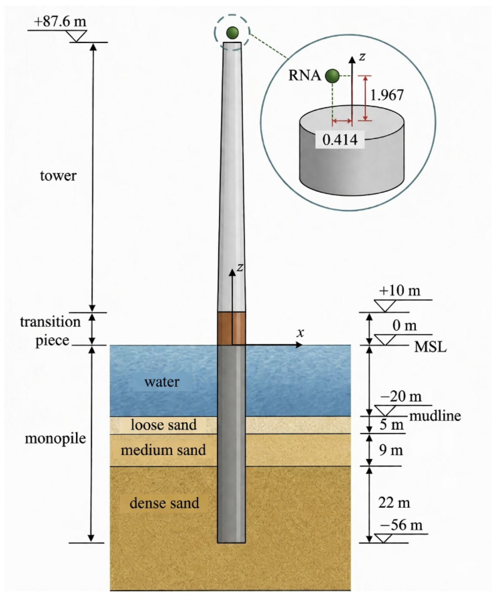
The subject of this study is the 5 MW monopile OWT developed by the National Renewable Energy Laboratory (NREL). It features an 87.6 m hub height and a 126 m rotor diameter [27]. The rotor-nacelle assembly is modeled as a lumped mass at the tower top, with specified mass moments of inertia. The tower is a tapered cylinder with its diameter and wall thickness decreasing linearly from 6 m and 27 mm at the base to 3.87 m and 19 mm at the top, respectively. A transition piece, maintaining a 6 m diameter while its thickness increases from 27 mm to 60 mm, connects the tower to the substructure. The supporting monopile (6 m diameter, 60 mm thickness) has a total length of 56 m, including a 36 m embedment into the seabed. Figure 1 illustrates the structural layout.

The supporting structure is composed of S355 steel, with its material properties listed in

Table 1. Pile material characteristics.

Property	Value
Young’s modules (GPa)	210
Poisson’s ratio	0.3
Density (kg/m3)	8500
Yield strength (MPa)	355

[27]. To account for the mass contributions of coatings, bolted connections, and flanges that are not explicitly modeled in the tower, an effective density of 8500 kg/m³ is adopted.

2.2. Soil-Structure Interaction Modeling

The p-y curve method is adopted to simulate the pile–soil interaction in this study, which has been widely applied in offshore foundation analysis due to its computational efficiency and its capability to reasonably capture soil–pile interaction behavior [28]. This approach represents the soil as a series of independent nonlinear springs distributed along the pile depth, based on the Winkler foundation idealization [29]. In this framework, the soil reaction per unit length p is expressed as a nonlinear function of the lateral pile displacement y through empirically derived p-y relationships.

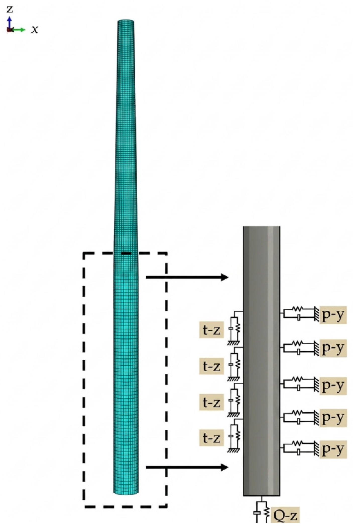
In the FEM, the monopile is discretized using shell elements, while the soil resistance is represented by a series of discrete nonlinear springs attached to the pile nodes along the embedded depth. The pile node is connected to an independent reference point through three types of springs: p-y springs (lateral response), t-z springs (axial shaft resistance), and Q-z springs (tip resistance). This modeling strategy enables the soil response in different directions to be captured in a decoupled yet depth-dependent manner, as illustrated in Figure 2.

The stiffness of the springs is determined based on the subgrade reaction modulus K, which varies with soil properties and depth. According to the geological profile shown in Figure 1, the seabed consists of multiple sand layers. The corresponding soil parameters adopted in the analysis are summarized in

Table 2. Properties of different sandy soil layers.

Soil Layer	Thickness (m)	E’ (Mpa)	γ’ (KN/m3)	Φ’ (°)	K (kN/m3)
Loose sand	5	30	10	33.0	16,287
Medium sand	9	35	10	35.0	24,430
Dense sand	36	47	10	38.5	35,288

.

2.3. Verification of Finite Element Model

To verify the reliability of the developed finite element model, its dynamic characteristics are evaluated through modal analysis and compared with reference results reported in the literature. The first two bending modes in both the side-side and fore-aft directions are selected as validation indicators due to their significance in the dynamic response of offshore wind turbines (OWTs). The natural frequencies of FEM are compared with reference values [30] in

Table 3. Natural frequency results for the 5 MW OWT (Hz).

Mode	Ref. [30]	Present	Difference (%)
1st side-side	0.249	0.254	2.01
1st fore-aft	0.248	0.257	3.62
2nd side-side	1.383	1.330	−3.83
2nd fore-aft	1.534	1.459	−4.89

. The first side-side frequency is 0.254 Hz, differing by 2.01% from the reference (0.249 Hz), while the first fore-aft frequency is 0.257 Hz (deviation 3.62% from 0.248 Hz). For the second-order modes, the side-side frequency is 1.330 Hz (deviation −3.83% from 1.383 Hz) and the fore-aft frequency is 1.459 Hz (deviation −4.98% from 1.534 Hz). The deviation in the first side-aside mode was the smallest, and all deviations less than 5% mean the FEM satisfies the engineering requirement. In static response verification, the tower-top horizontal displacement under representative loading showed a deviation of less than 5% from the reference, confirming the model’s ability to capture global stiffness with acceptable accuracy. Thus, the model’s capability to represent both dynamic and static structural behavior is validated, making it suitable for subsequent analyses.

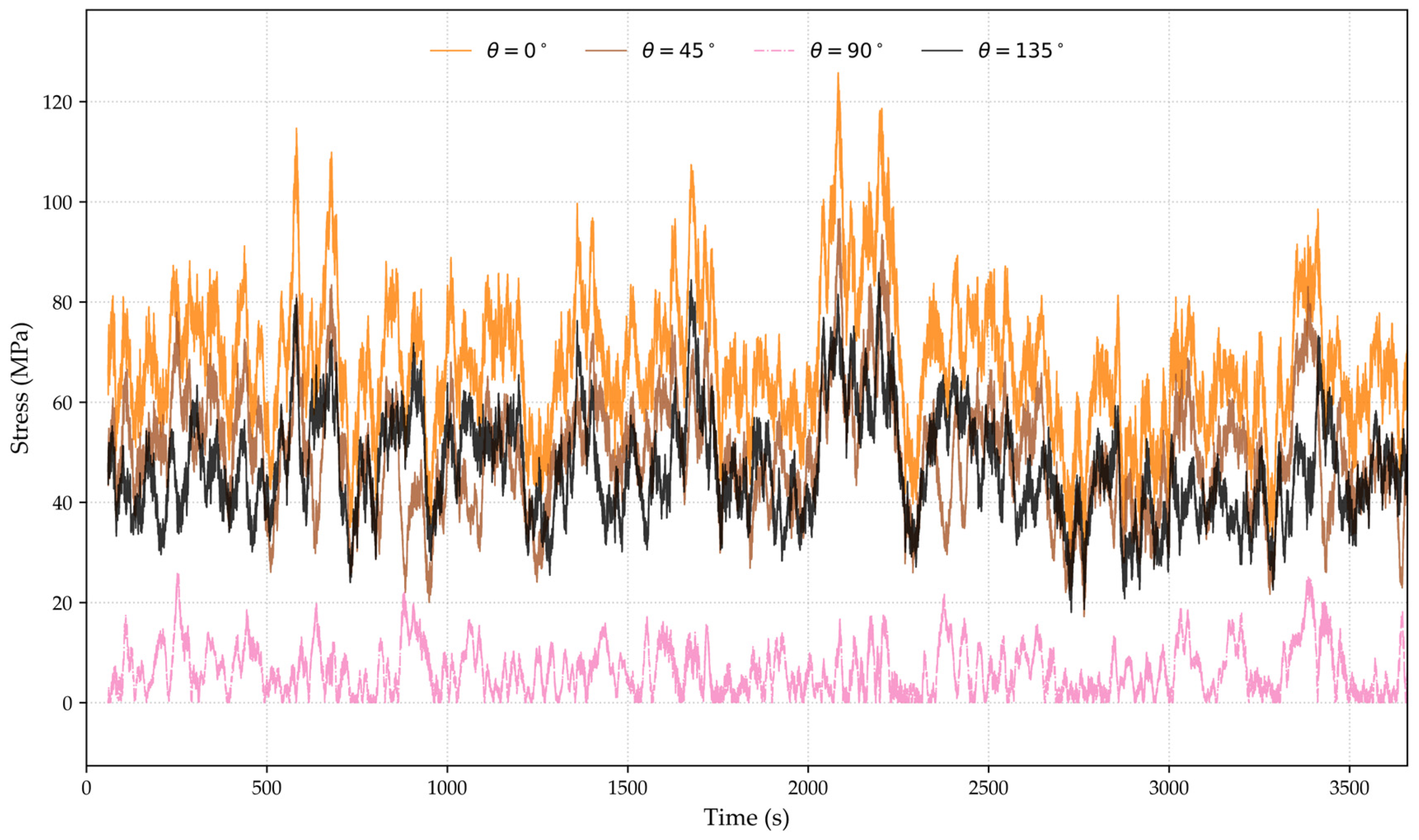
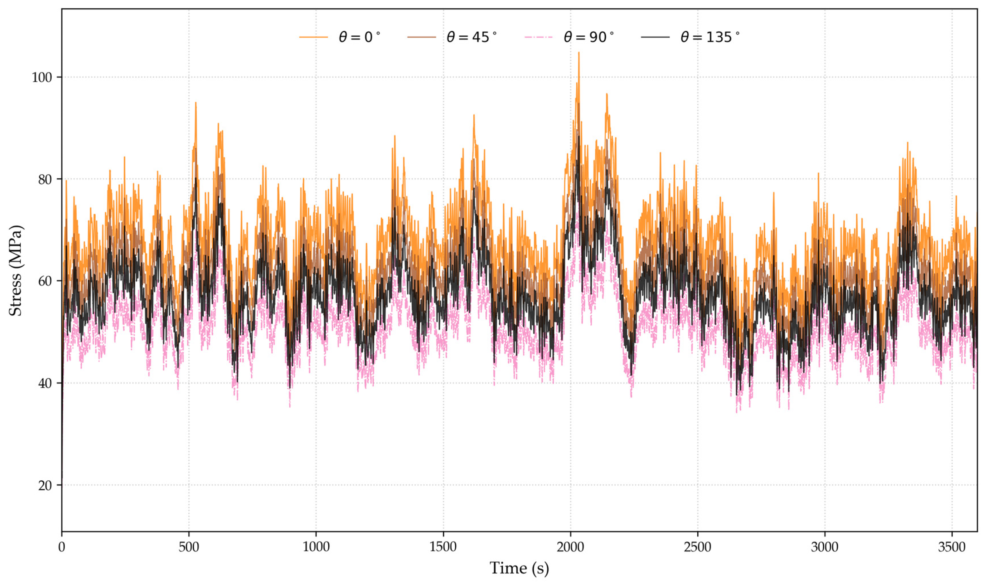
To further verify the validity of the model, the time-history curves of maximum principal stress at various angles at the foundation mudline were calculated using OpenFAST and FEM, as shown in Figure 3 and Figure 4. The maximum damages at the foundation mudline computed by the FEM and OpenFAST are 9.1 × 10⁻⁶ and 8.8 × 10⁻⁶, respectively, with an error of less than 5%. Therefore, the proposed model can be applied for subsequent calculations.

3. Fatigue Damage Estimation of OWT Foundation

3.1. Wind and Wave Load

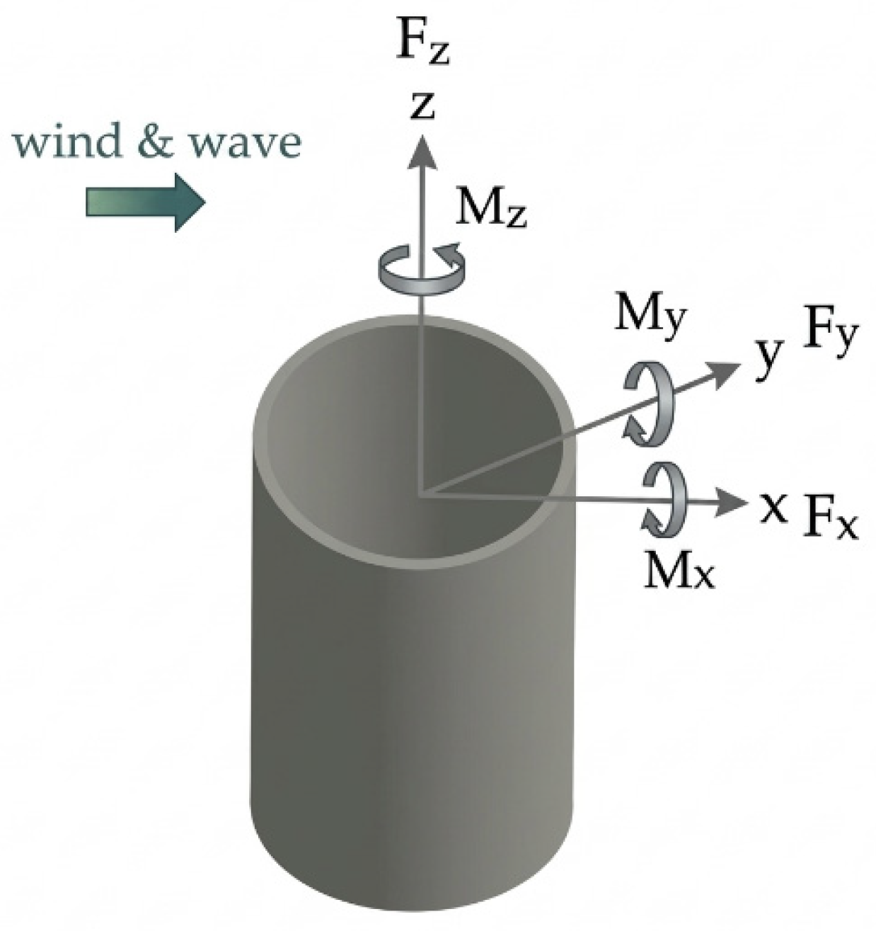
Wind and wave loads acting on OWT monopile foundation constitute the primary sources of cyclic stresses responsible for fatigue damage. In the present study, these loads are simulated in the time domain using the spectral representation approach [31] implemented in the AeroDyn and HydroDyn modules of OpenFAST ,with their positive directions illustrated in Figure 5. The total simulation duration is set to 3660 s, with the initial 60 s discarded to eliminate start-up transients. Subsequently, a 600 s segment of the stabilized wind and wave load time histories is extracted and applied to the FEM for fatigue analysis.

The turbulent wind field is generated based on Normal Turbulence Model (NTM) specified in the IEC 61400-1 for wind conditions Class B [32]. Atmospheric turbulence is characterized using the one-sided Kaimal power spectral density function, expressed as:

$$S_k(f)={\displaystyle \frac{4{\sigma }_k^2{L}_k/U_{hub}}{{\left(1+6f{L}_k/U_{hub}\right)}^{5/3}}},$$

(1)

where $f$ is the frequency, $U_{hub}$ is the hub-height wind speed, which is taken as the stochastic environmental parameter in the fatigue-oriented parametric study. ${\sigma }_k$ and $L_k$ denote the standard deviation of the respective velocity component and the turbulence integral length scale respectively, defined as:

$$L_k=\left\{\begin{array}{c}8.1z_{\mathit{hub}},k=x\\ 2.7z_{\mathit{hub}},k=y\\ 0.66z_{\mathit{hub}},k=z\end{array}\right.,$$

(2)

where $I_{ref}=0.14$ for wind conditions of Class B, $z_{hub}$ is the hub height of the wind turbine.

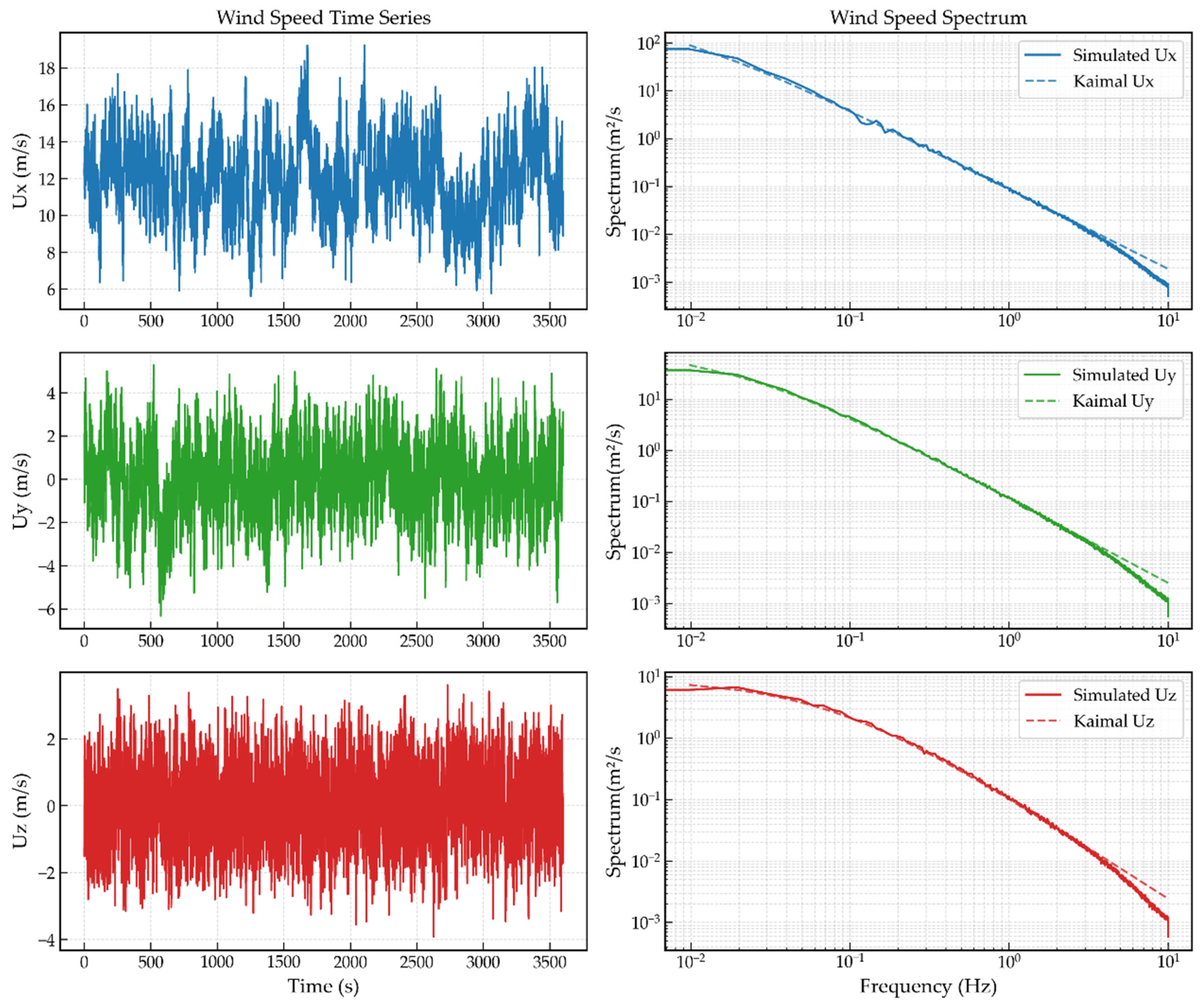
Considering that the operational wind speed of the turbine ranges from 4 to 18 m/s, a representative wind speed of 12 m/s is selected to generate the three-component turbulent velocity field. Figure 6 presents the time histories and spectra of the longitudinal (Ux), lateral (Uy), and vertical (Uz) wind components. It can be observed that Ux fluctuates around 12 m/s, while Uy and Uz oscillate about zero. The spectra of all three components exhibit a consistent decay trend across the entire frequency range. Although the energy levels of Uy and Uz are lower than that of Ux, their spectral shapes are in good agreement with the Kaimal theoretical spectrum. This confirms that the generated turbulent wind field reliably captures the multi-directional nature of atmospheric turbulence for subsequent load simulations.

The aerodynamic load acting on the rotor is simplified as an equivalent thrust force obtained from OpenFAST and applied at the rotor-nacelle assembly (RNA) along the wind direction [33]. Meanwhile, the wind load acting on the tower is modeled as distributed surface pressure on the windward side, calculated according to:

$$P_w(z)={\displaystyle \frac{1}{2}}\rho C_p{U_{wind}}^2(z),$$

(3)

where $\rho$ is the air density, $C_p$ is the coefficient of wind pressure. The wind speed at any height x of the tower $U_{wind}$ is defined as:

$$U_{wind}(z)=U_{hub}{(z/z_{hub})}^{\alpha },$$

(4)

where U_hub is the hub-height wind speed, $\alpha$ is the exponent of mean wind speed profile on the sea equaling 0.115 [34].

Wave-induced loads are simulated using an irregular wave model based on spectral representation [31], which enables a realistic description of stochastic ocean wave conditions. In this study, the wave field is generated in the HydroDyn module of OpenFAST using the Joint North Sea Wave Project (JONSWAP) spectrum, which is widely adopted for wind-generated seas [26]. The wave energy spectrum is defined as:

$$S(\omega )=\alpha g^2{\omega }^{-5}\exp \left[-{\displaystyle \frac{5}{4}}{\left({\displaystyle \frac{{\omega }_p}{\omega }}\right)}^4\right]{\gamma }^{\exp \left[-{\displaystyle \frac{{(\omega -{\omega }_p)}^2}{2{\sigma }^2{\omega }_p^2}}\right]},$$

(5)

where $\omega$ is the angular frequency, ${\omega }_p$ is the peak frequency, and $\alpha$, $\gamma$, and $\sigma$ are empirical parameters controlling the spectral shape.

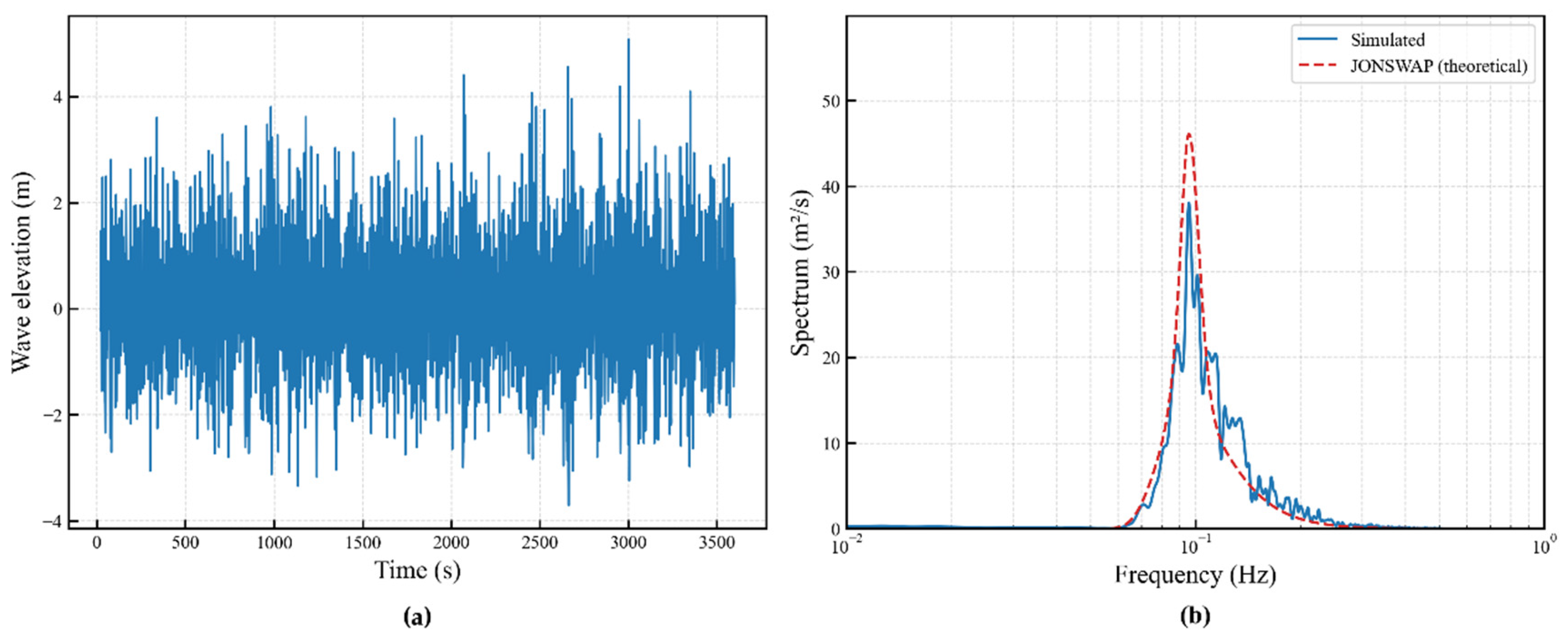
A representative irregular wave condition with a significant wave height of H_s = 5 m and a peak period of T_p = 10 s is considered, as illustrated in Figure 7a. The generated wave elevation time history exhibits a zero-mean characteristic, consistent with the stochastic nature of irregular waves. To further validate the wave simulation, a Fourier transform is applied to the generated wave elevation time series to obtain the corresponding wave spectrum. As shown in Figure 7b, the simulated spectrum closely matches the theoretical JONSWAP spectrum in both spectral shape and magnitude, confirming the accuracy of the wave generation method.

The total horizontal wave force and the corresponding bending moment at the seabed are obtained by integrating the distributed hydrodynamic loads along the submerged length of the monopile, as expressed in:

$$F_{total}(t)={\displaystyle \sum _{i=1}^{N}F}(z_i,t)\Delta z_i,$$

(6)

$$M_{base}(t)={\displaystyle \sum _{i=1}^{N}F}(z_i,t)(z_i+h)\Delta z_i,$$

(7)

The hydrodynamic forces acting on the monopile $F(z,t)$ are calculated using Morison’s equation, which accounts for both drag and inertia effects:

$$F(z,t)={\displaystyle \frac{1}{2}}\rho C_{d}D|u(z,t)|u(z,t)+\rho C_m{\displaystyle \frac{\pi D^2}{4}}\dot{u}(z,t),$$

(8)

where $\rho$ is the water density, $C_d$ and $C_m$ are the drag and inertia coefficients respectively, and $D$ is the monopile diameter. $u(z,t)$ is the horizontal water particle velocity; assuming linear wave theory, it can be defined as:

$$u(z,t)={\displaystyle \sum _{i=1}^N\frac{{\omega }_i\cosh k_i(z+h)}{\sinh (k_{i}h)}}{A}_i\cos ({\omega }_{i}t+{\varphi }_i),$$

(9)

where $k_i$ is the wave number corresponding to ${\omega }_i$, $h$ is the water depth, and $A_i$ is the wave amplitude of each component.

3.2. Parametric Design of Wind–Wave Conditions

To establish a fatigue database for surrogate model training, representative environmental conditions are selected, namely hub-height wind speed U_hub, significant wave height H_s, and peak wave period T_p. As shown in

Table 4. Ranges of environmental parameters used in the present study.

Parameter	Symbol	Range
Hub-height wind speed	Uhub	4–18 m/s
Significant wave height	Hs	1–8 m
Peak wave period	Tp	4–14 s

, U_hub ranges from 4 to 18 m/s, covering typical operating conditions from near cut-in to moderate wind regimes that contribute substantially to fatigue damage; H_s is used to characterize sea state severity and is considered within the range of 1–8 m; and T_p is set from 4 to 14 s to capture typical offshore wave conditions and potential resonance effects. Although these parameters are correlated in real sea states, treating them as independent variables within physically reasonable ranges avoids limiting the parameter space and enhances surrogate model generalization.

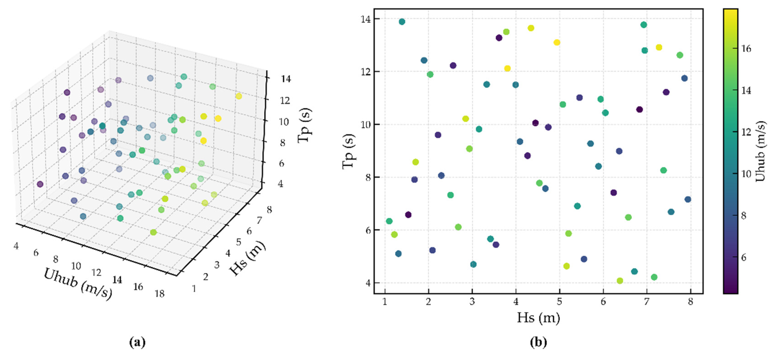
Latin Hypercube Sampling (LHS) is employed to generate 60 uniformly distributed samples across the three-dimensional parameter space in Figure 8. For each sample, wind and wave load time histories are generated using aerodynamic and hydrodynamic models in Section 3.1, and incorporated into the FEM for dynamic simulations to evaluate the fatigue damage of the OWT foundation. These data form the basis for subsequent surrogate model development.

3.3. Framework of Fatigue Damage Estimation Method

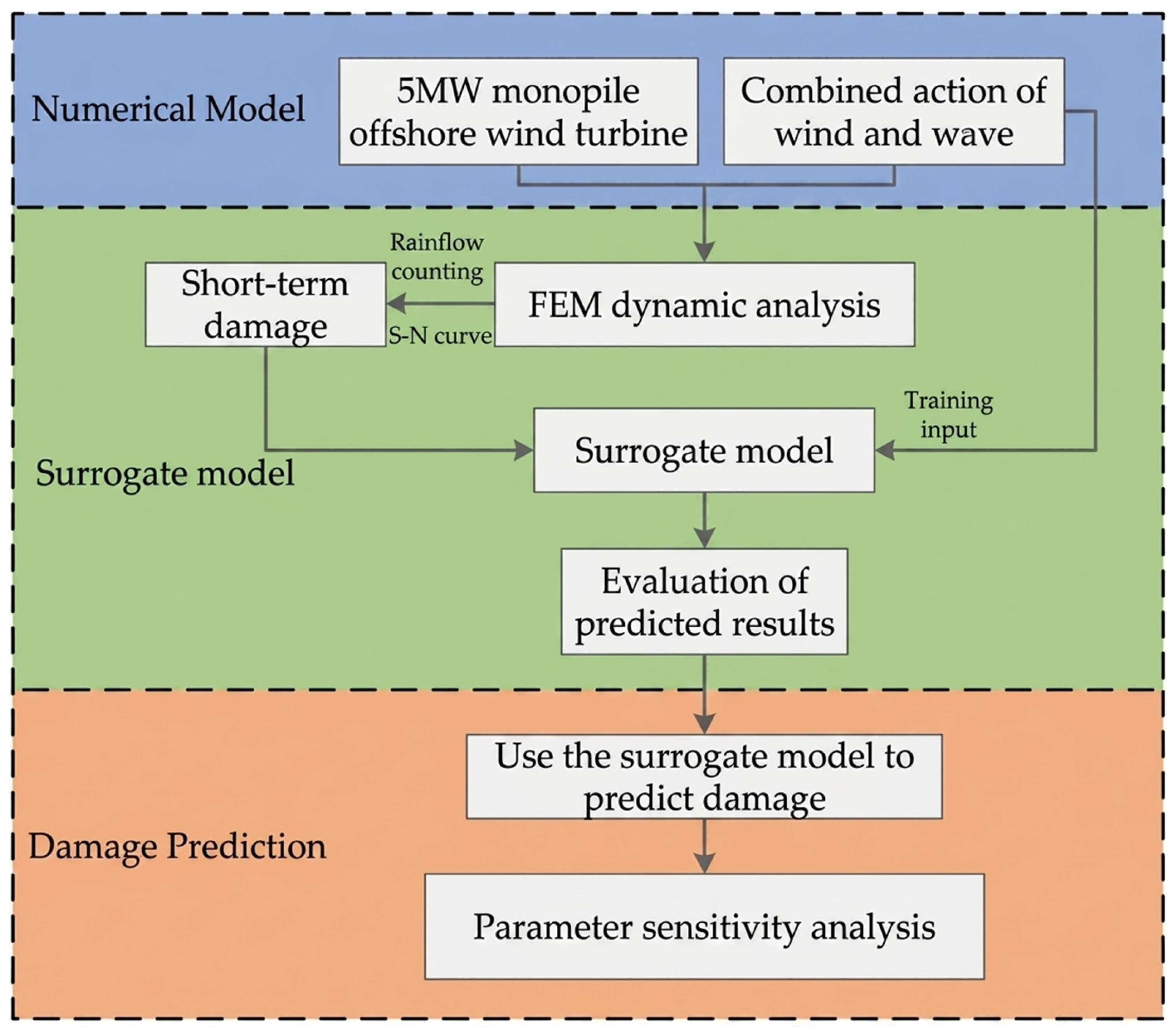
The overall framework for fatigue damage estimation of OWT foundation is illustrated in Figure 9. First, transient dynamic simulations are conducted for 600 s under combined wind and wave loading using the finite element model (FEM). Second, short-term fatigue damage is evaluated by rainflow counting combined with the S-N curve. Next, an optimized surrogate model is constructed to map environmental parameters to fatigue damage. Finally, the fatigue characteristics of the foundation are analyzed under combined wind–wave conditions.

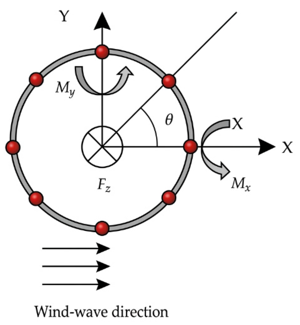
For monopile-supported offshore wind turbines, fatigue damage is primarily governed by cyclic bending stresses near the mudline, where maximum bending moments occur. In this study, a reference cross-section at an elevation of −20 m is selected as the fatigue-critical section, corresponding to the pile–soil interaction zone where significant cyclic loading is induced. To capture the circumferential variation in stress, eight angular positions are defined along the pile perimeter, where $\theta =\left\{0^{°},{45}^{°},{90}^{°},{135}^{°},{180}^{°},{225}^{°},{270}^{°},{315}^{°}\right\}$ as shown in Figure 10.

Fatigue assessment approaches based on stress ranges are widely adopted for offshore wind turbine (OWT) structures under coupled loading conditions, particularly when multiaxial stress states are involved [35,36,37]. In accordance with the recommendations of DNV GL RP-C203 for welded steel structures, the fatigue damage of the OWT foundation in this study is evaluated based on the maximum principal stress [38].

The pile is established by shell elements in FEM. For shell elements, the formula for calculating the maximum principal stress at the position of angular $\theta$ is as follows:

$${\sigma }_{\theta }(t)={\displaystyle \frac{{\sigma }_x(t)+{\sigma }_y(t)}{2}}+\sqrt{{({\sigma }_x(t)-{\sigma }_{\mathrm{y}}(t))}^2+{\tau }_{xy}{(t)}^2},$$

(10)

where ${\sigma }_x$, ${\sigma }_y$ and ${\tau }_{xy}$ correspond to the axial normal stress, circumferential normal stress and in-plane shear stress respectively in the local coordinate system.

The stress time histories are processed using the rainflow counting method to decompose irregular loading into discrete stress cycles [39]. For each circumferential angle, the sequence of stress turning points is identified, and rainflow counting is applied to determine the stress range $\Delta {\sigma }_i$ and the corresponding number of cycles $n_i$. In accordance with the DNV GL recommended practice for offshore welded steel structures, the mean stress effect is neglected, and the stress range is adopted as the governing fatigue parameter [38]. Fatigue damage of OWT foundation is evaluated based on Miner’s linear damage accumulation rule:

$$D={\displaystyle \sum _i\frac{n_i}{N_i}},$$

(11)

where N_i denotes the allowable number of cycles to failure under the stress range $\Delta {\sigma }_i$. The value of N_i is obtained from the S-N curve of DNV GL E class [38], which is appropriate for tubular steel structures subjected to offshore environmental loading. The S-N relationship is expressed as:

$$N_i=C\cdot \Delta {{\sigma }_i}^{-m},$$

(12)

where m is the inverse slope of the S-N curve and C is the fatigue strength coefficient. According to the DNV GL Class E specification, m = 3 and logC = 11.755.

The cumulative fatigue damage is computed at each circumferential angle, and the maximum value among all angles is taken as the representative fatigue damage index for the given environmental condition:

$$D_{\mathrm{rep}}={\max }_{\theta }{\displaystyle \sum _i\frac{n_i(\theta )}{N_i(\Delta {\sigma }_i(\theta ))}},$$

(13)

which is subsequently used as the output variable for surrogate model training and parameter optimization in Section 4.

4. Surrogate-Assisted Fatigue Damage Estimation of OWT Foundation

4.1. Performance Evaluation of the Surrogate Models

In offshore wind turbine systems subjected to complex wind and wave conditions, the mapping from environmental inputs to foundation fatigue response is strongly nonlinear. According to IEC 61400-3-1, wind speed intervals should be smaller than 2 m/s, wave height intervals should be less than 0.5 m, and wave period intervals should be less than 0.5 s for fatigue damage estimation [32]. Considering the parameter settings in Section 3.2, at least 2500 finite element simulations under different environmental conditions are required in fatigue damage estimation, resulting in substantial computational effort.

Four surrogate models are introduced to mitigate this limitation: Extreme Gradient Boosting (XGBoost), Random Forest (RF), Support Vector Regression (SVR), and Gaussian Process Regression (GPR). These models are widely used in nonlinear regression problems and have demonstrated strong performance in wind energy applications. For model development, a dataset consisting of 60 environmental conditions is generated as described in Section 3.2, among which 45 samples are used for training and 15 samples are used for validation. The surrogate models are constructed to establish an efficient predictive relationship between environmental conditions and fatigue response. XGBoost has demonstrated strong performance in nonlinear regression and engineering prediction tasks, particularly for high-dimensional and complex datasets. Each new tree is trained to capture the residuals of the existing ensemble, enabling sequential model construction. The learning process aims to minimize an objective function consisting of a loss term and a regularization term, which jointly control the fitting error and model complexity [40,41]. For tree-based learners, the model prediction can be expressed as the summation of multiple regression trees:

$${\widehat{y}}_i={\displaystyle \sum _{k=1}^K{f}_k(x_i}),f_k\in F,$$

(14)

where K indicates the number of trees and $f_k$ corresponds to a regression tree. In this context, the maximum tree depth determines the complexity of individual trees, while the K controls the ensemble size and prediction stability. The evaluation adopts the mean absolute percentage error (MAPE), expressed as:

$$MAPE={\displaystyle \frac{1}{N}}{\displaystyle \sum _{i=1}^N{\left|\frac{p_i^e-{p_i}^s}{{p_i}^s}\right|}^2},$$

(15)

where p^e denotes the predicted value, p^s denotes the simulated value from FEM.

As shown in

Table 5. Impact of the tree numbers K on XGBoost model performance.

K	MAPE	RE
100	51.44	37.44
200	34.24	24.21
300	33.29	22.76
500	33.29	22.76
1000	33.29	22.76

, the MAPE of the XGBoost model decreases with an increasing number of trees K and gradually converges to 33.29% when the number of trees reaches 300. Meanwhile, it is observed that the prediction accuracy is relatively insensitive to the maximum tree depth. This behavior can be attributed to the use of a small learning rate combined with a large number of trees, under which the model effectively behaves as an ensemble of weak learners, thereby improving robustness and reducing the risk of overfitting.

Random Forest (RF) is an ensemble learning method that constructs multiple decision trees through bootstrap sampling and random feature selection [42]. The final prediction is generated by aggregating the outputs from individual trees. RF has demonstrated strong robustness against overfitting and good performance in high-dimensional and nonlinear problems due to its ensemble and randomization mechanisms [43,44,45].

Table 6. Impact of the tree numbers K on RF model performance.

K	MAPE	RE
40	32.46	3.27
60	29.69	3.18
80	30.58	2.17
100	31.29	3.34
200	31.84	3.74
300	31.31	3.79
500	31.48	3.42

presents the relationship between the MAPE and the number of trees K in the RF model, with the maximum tree depth fixed at 16. The MAPE initially decreases with the increases in the number of trees, indicating improved model stability, and then slightly increases after reaching an optimal value, with the minimum error occurring at 60 trees. This behavior suggests that an excessive number of trees may introduce redundancy without further improving predictive performance.

Table 7. Effect of the maximum tree depth D_max on RF model performance.

Dmax	MAPE	RE
4	30.76	2.67
6	29.84	3.33
8	29.69	3.19
10	29.69	3.18
12	29.69	3.18
16	29.69	3.18

presents the effect of tree depth D_max on the prediction accuracy when the K is fixed at 80. It can be observed that the MAPE increases as the tree depth increases, and gradually converges when D_max reaches 8, achieving a minimum MAPE of 29.69%. This trend indicates that overly complex trees may lead to overfitting, while a moderate depth provides a better balance between model complexity and generalization ability.

Support Vector Regression (SVR) is a regression variant of Support Vector Machines (SVM). It has demonstrated strong capability in handling nonlinear relationships, particularly in small-sample and high-dimensional problems, and has been widely applied in energy-related prediction tasks [46,47,48]. SVR maps input data into a high-dimensional feature space using kernel functions (in this study, the radial basis function (RBF) kernel is adopted) and constructs an optimal hyperplane for regression [49]. The model is formulated by minimizing a regularized risk function that balances model flatness and training error, which can be expressed as:

$${\displaystyle \frac{1}{2}}{\Vert w\Vert }^2+C{\displaystyle \sum ({\xi }_i+{\xi }_i^{\ast })}$$

(16)

For SVR, the regularization parameter C controls the trade-off between model complexity and training error, while the kernel coefficient γ of the RBF kernel determines the influence range of individual training samples [5]. In addition, the parameter ε defines the width of the insensitive loss region.

Table 8. Effect of the penalty coefficient C on SVR model performance.

C	MAPE	RE
20	7.86	5.43
40	8.02	5.80
80	8.08	5.76
100	7.82	5.5
150	8.12	4.94
200	9.14	4.4
300	10.61	3.42

presents the relationship between the MAPE of the SVR model and the penalty coefficient C when the kernel coefficient γ = 0.1. The MAPE is observed to initially decrease and reaches its minimum when C = 100, indicating an optimal balance between underfitting and overfitting.

Table 9. Effect of the kernel coefficient γ on SVR model performance.

γ	MAPE	RE
0.1	7.82	5.5
0.2	12.44	8.81
0.4	18.45	16.99
1	20.95	28.31

shows the effect of the kernel coefficient γ on model performance. The results indicate that the MAPE increases with increasing γ, suggesting that overly localized kernel functions may reduce generalization capability. When C = 100 and γ = 0.1, the model achieves the best performance with a minimum MAPE of 7.81%.

Gaussian Process Regression (GPR) has demonstrated strong capability in load and fatigue prediction in OWT due to its probabilistic nature and ability to quantify prediction uncertainty [50]. It is a non-parametric Bayesian approach that models the relationship between input variables and output responses as a Gaussian process defined by a mean function and a covariance (kernel) function [51]. The prediction at a new point follows a Gaussian distribution, providing both the mean estimate and the associated uncertainty, which is particularly advantageous for engineering applications involving stochastic environmental conditions.

In this study, a composite kernel function consisting of a constant kernel of RBF and a white noise term is adopted to capture the global trend, nonlinear variations, and noise in the data, respectively, which can be defined as:

$$k(x,x^{\prime })=C\cdot \exp \left(-{\displaystyle \frac{\Vert x-x^{\prime }{\Vert }^2}{2l^2}}\right)+{\sigma }_n^2$$

(17)

For the GPR model, the kernel hyperparameters, including the length-scale $l$, are automatically optimized during training via maximum likelihood estimation. Consequently, the influence of initial parameter selection on model performance is relatively limited, and the model tends to converge toward an optimal configuration. In this study, the GPR model exhibits stable predictive performance, with the MAPE remaining approximately 7.51%.

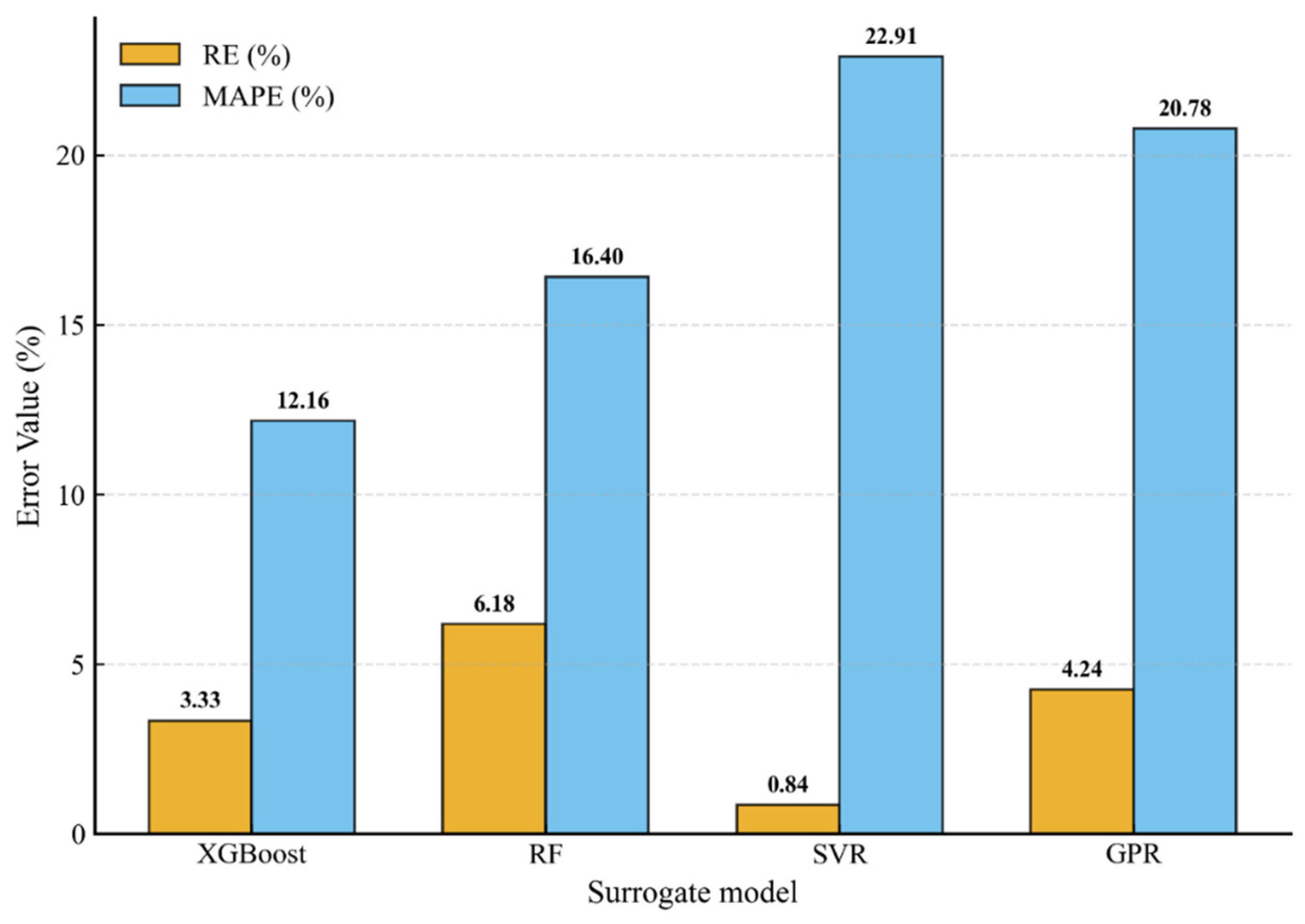
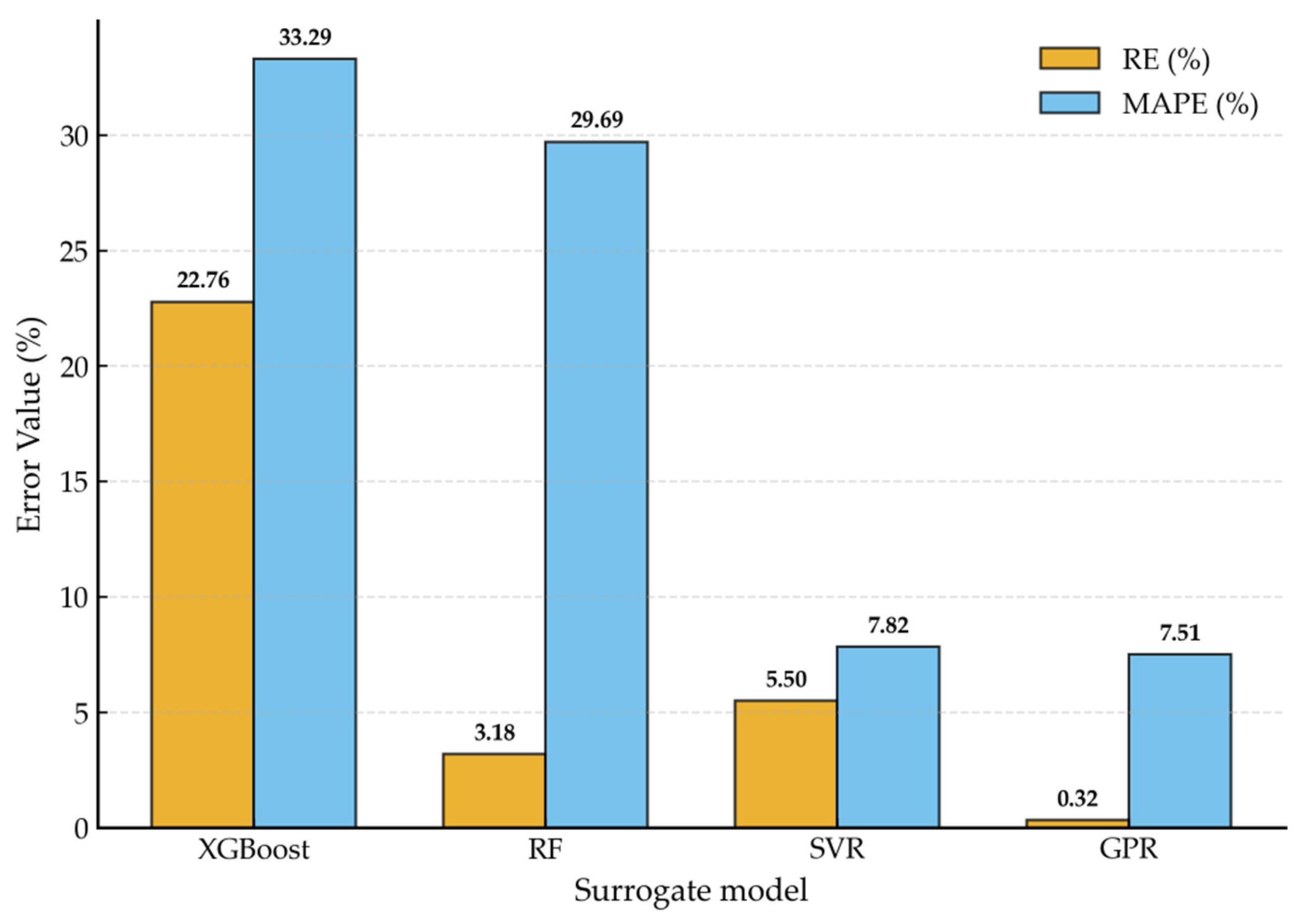
A comparison of the predictive accuracy of the four surrogate models is shown in Figure 11. It can be observed that the GPR model achieves the lowest MAPE (7.51%), indicating the highest prediction accuracy among all models. The SVR model shows comparable performance, with a slightly higher error of 7.82%. In contrast, the RF and XGBoost models exhibit relatively larger prediction errors, suggesting a lower capability in capturing the underlying nonlinear relationships of fatigue damage.

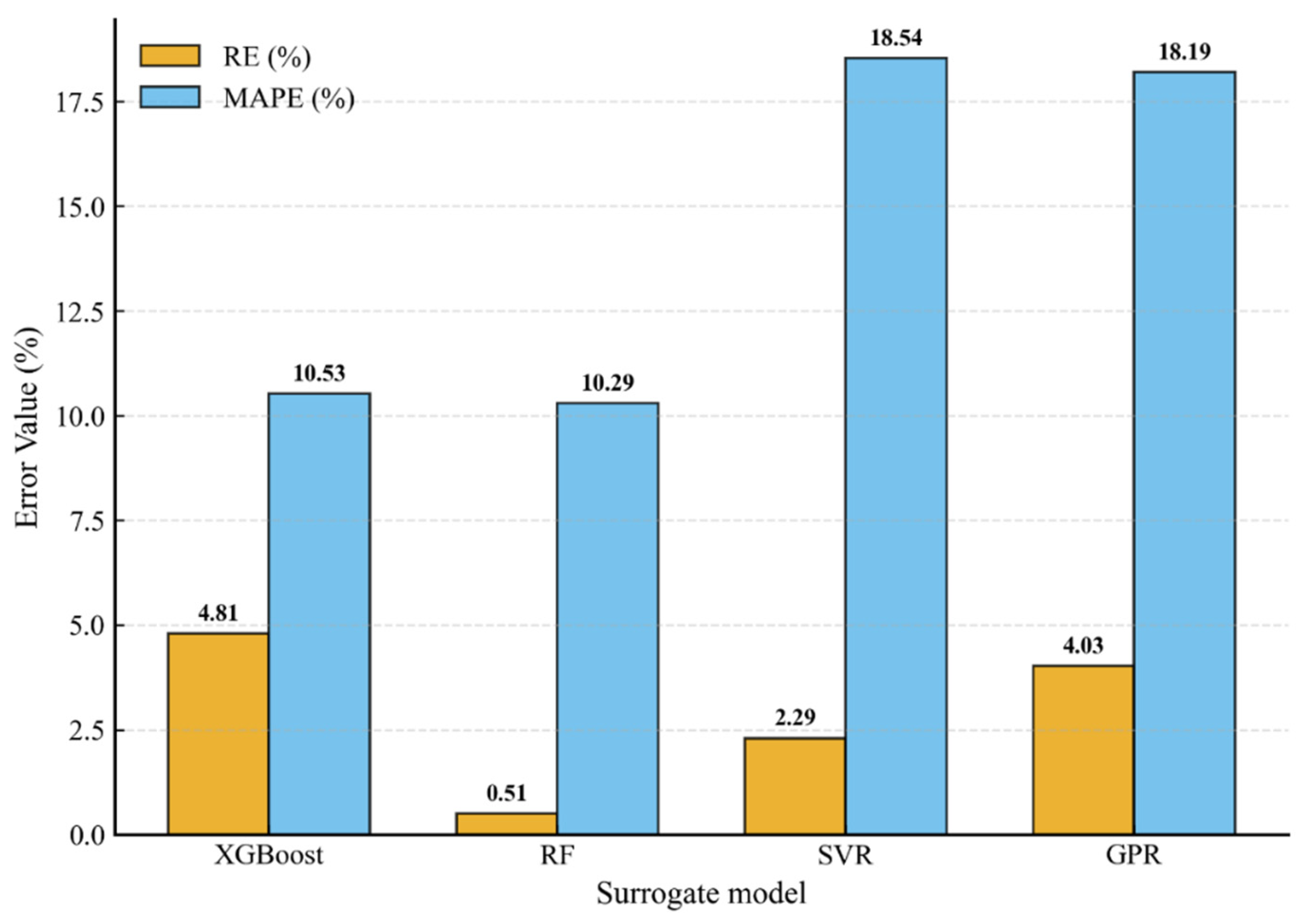
In addition, Figure 12 and Figure 13 present the MAPE and RE values of the four models at 180 and 300 sample points, respectively. It can be observed that the MAPE of the XGBoost and RF models decreases with increasing sample size, converging to 10.53 and 10.29 at 300 sample points, respectively, indicating their suitability for prediction when sufficient sample points are available. In contrast, the errors of the SVR and GPR models do not decrease with increasing sample size; instead, they achieve the highest accuracy at 60 sample points. This suggests that their representation capacity is limited by the kernel’s ability to capture complex interactions, and more flexible kernels might be needed for larger datasets. In conclusion, GPR is the preferred choice when the available simulation budget is very limited and interpretable uncertainty is desired. For scenarios where large amounts of data can be generated, XGBoost or RF may eventually outperform GPR.

The evaluation employs the root mean square error (RMSE) and the correlation coefficient (R) to further evaluate the predictive performance, which are defined as:

$$RMSE=\sqrt{{\displaystyle \frac{1}{N}}{\displaystyle \sum _{i=1}^N{\left|p_i^e-\overline{{p_i}^s}\right|}^2}},$$

(18)

$$R={\displaystyle \frac{{\displaystyle \sum _{i=1}^N(p_i^e-\overline{p^e})(p_i^f-\overline{p^f})}}{\sqrt{\frac{1}{N}{\displaystyle \sum _{i=1}^N{\left|p_i^e-\overline{p^e}\right|}^2}}\times \sqrt{\frac{1}{N}{\displaystyle \sum _{i=1}^N{\left|p_i^f-\overline{p^f}\right|}^2}}}}$$

(19)

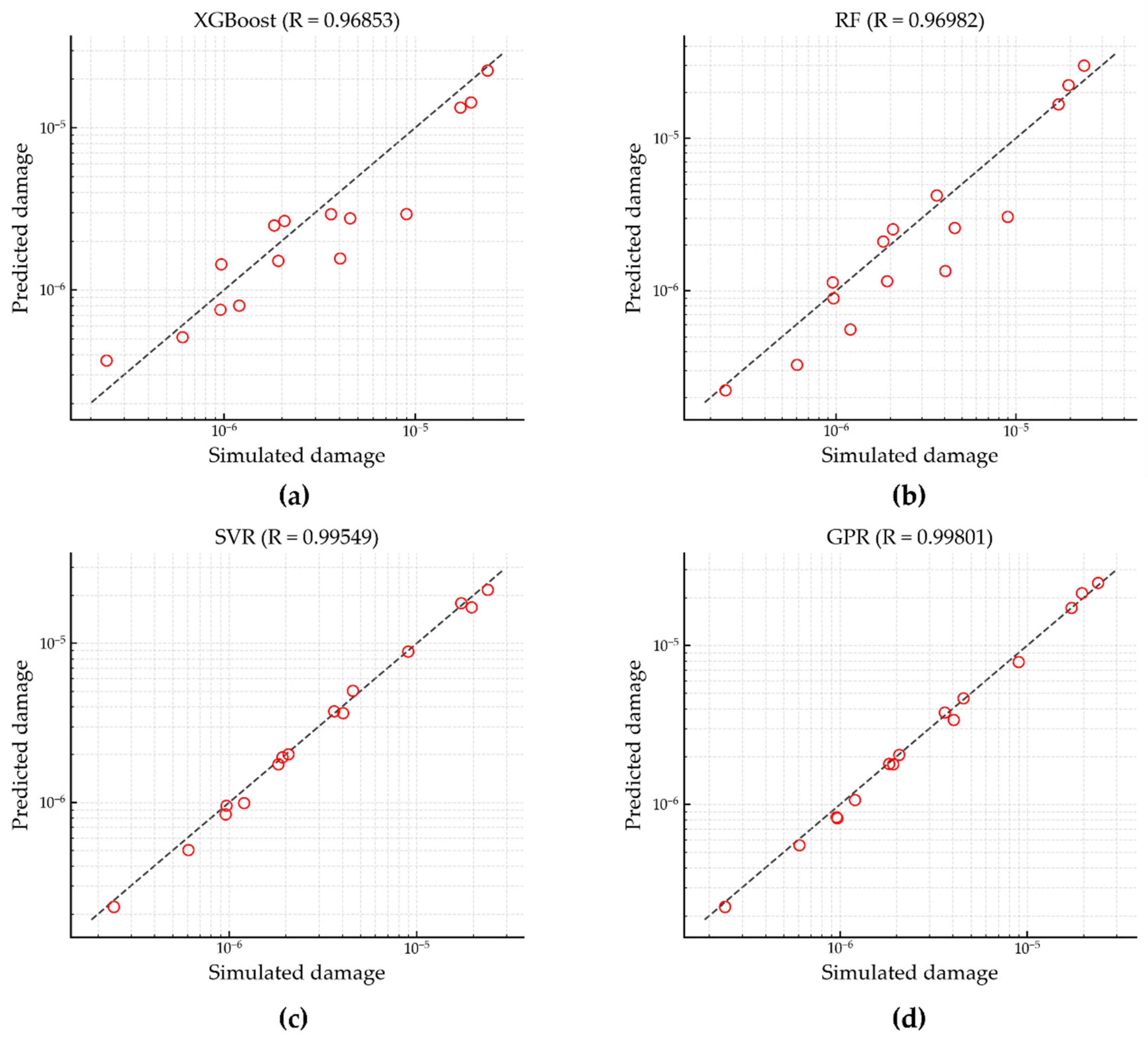
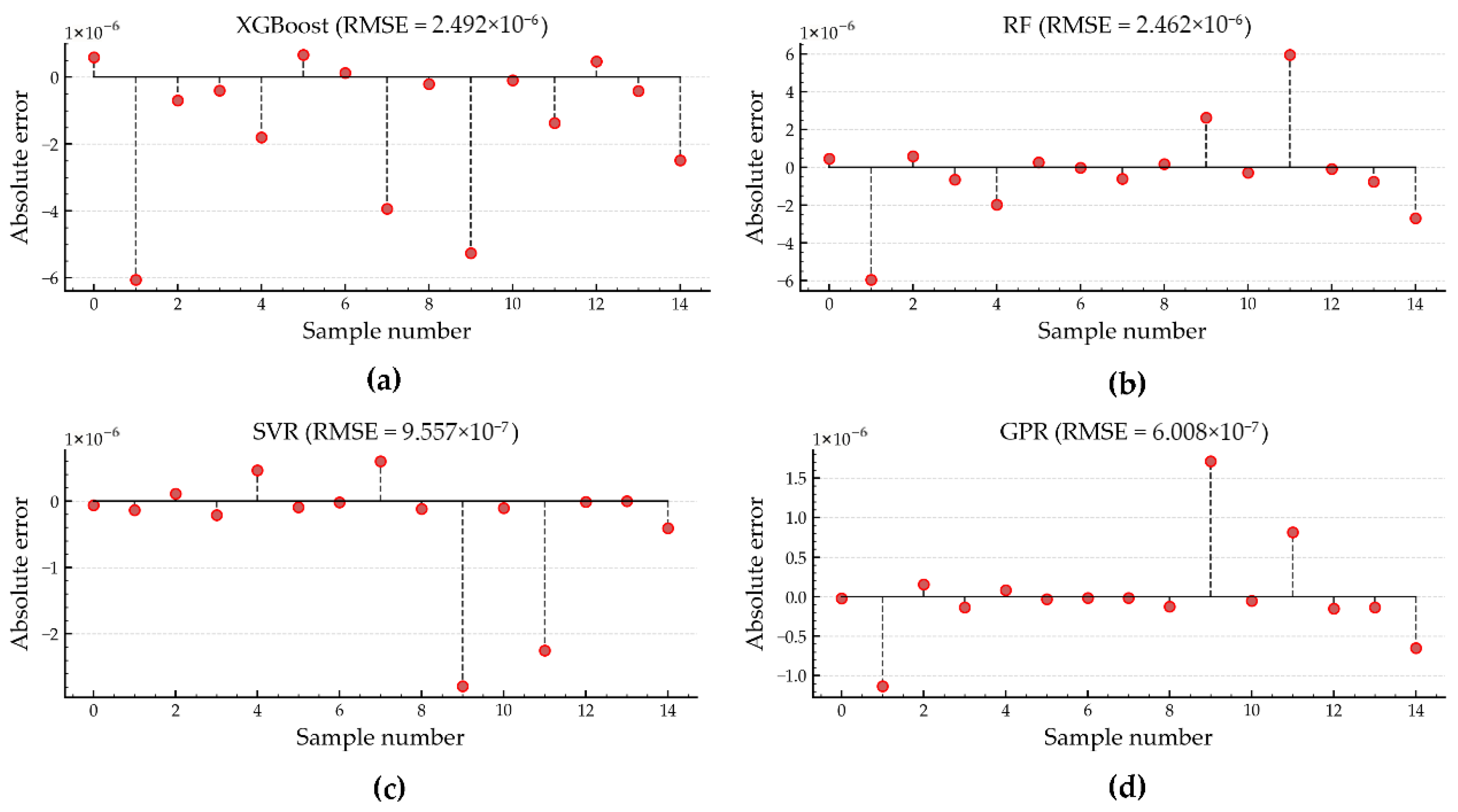
RMSE is used to measure the difference between predicted values and observed values; R serves as a measure of the model’s goodness of fit; a value approaching 1 reflects higher predictive accuracy. The result illustrated in Figure 14 and Figure 15 for the testing dataset based on 45 training samples demonstrates that the GPR and SVR models consistently achieve lower RMSE values and higher correlation coefficients compared to the RF and XGBoost models, indicating superior fitting accuracy and generalization capability.

In contrast, larger prediction errors are observed for the tree-based models, particularly in cases involving complex nonlinear responses. In addition to point-wise error metrics, the total error of short-term fatigue damage RE for the 15 testing cases is evaluated in Figure 11. which is defined as the absolute percentage error between the cumulative fatigue damage predicted by the surrogate models and that obtained from FEM:

$$RE=\left|{\displaystyle \frac{{\displaystyle \sum _{i=1}^n{p}_i^{\mathrm{e}}-{\displaystyle \sum _{i=1}^n{p}_i^s}}}{{\displaystyle \sum _{i=1}^n{p}_i^s}}}\right|\times 100\%,n=15$$

(20)

The study reveals that the RE values are much lower than the MAPE values, as overestimations in some samples and underestimations in others cancel each other out, yielding a small RE. Among the four models, the GPR model achieves the lowest relative error of 0.32%.

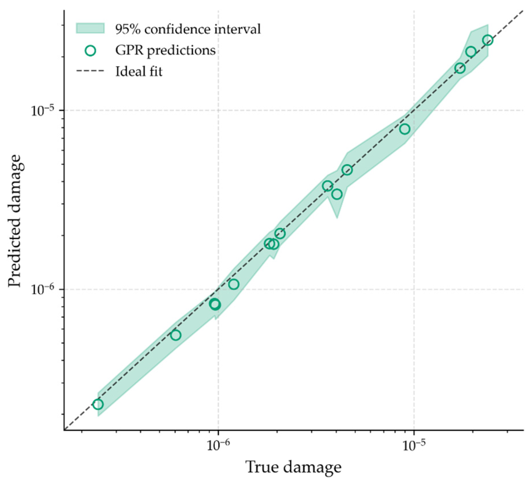
Figure 16 compares the predicted and true fatigue damage using the GPR model, with 95% prediction intervals. Most points lie within these intervals, confirming reliable uncertainty quantification. The interval width reflects model confidence: narrower intervals indicate sufficient training data, while wider ones signal greater uncertainty. This highlights GPR’s ability to capture both prediction accuracy and associated uncertainty.

Compared with the 2520 load cases required by the IEC 61400-3-1 standard [32], only 60 representative environmental conditions need to be simulated in this study, while the remaining cases can be efficiently estimated using surrogate models. The computational cost of surrogate prediction is negligible compared to FEM-based transient simulations.

4.2. Sensitivity of OWT Foundation Fatigue Damage to Environmental Parameters

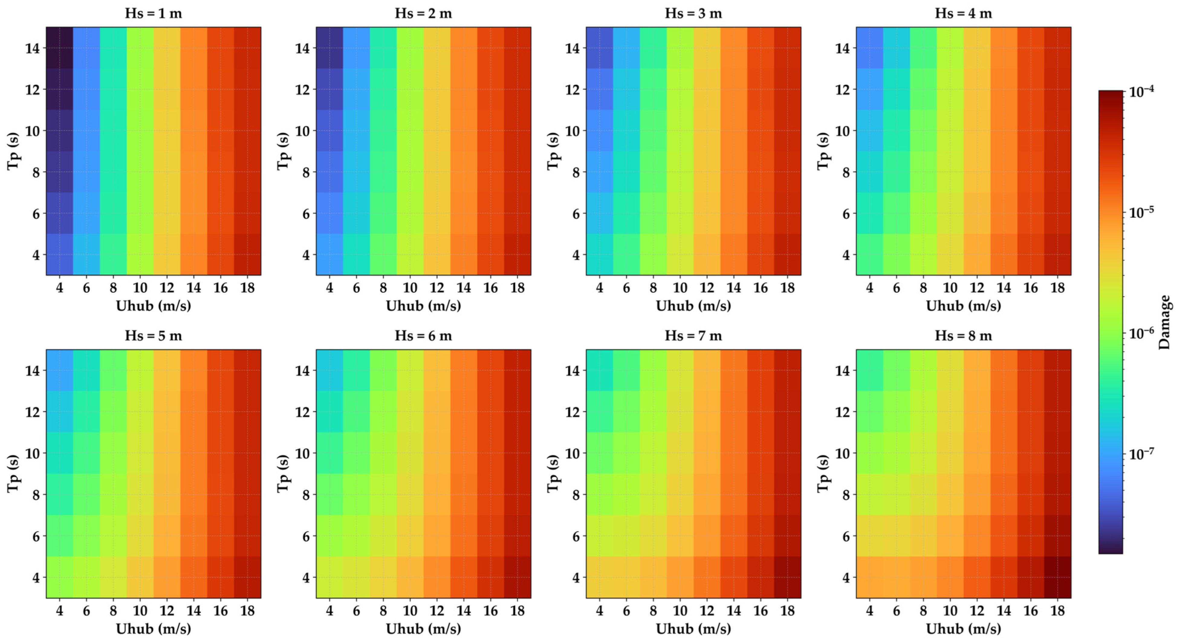
Based on model comparison, the GPR model, identified as the most accurate surrogate, is selected to evaluate the influence of environmental parameters on foundation fatigue damage. A total of 384 environmental conditions are evaluated, with U_hub ranging from 4 to 18 m/s (interval of 2 m/s), H_s from 1 to 8 m, and T_p from 4 to 14 s, covering a wide range of representative offshore operating conditions.

As shown in Figure 17, fatigue damage exhibits a clear increasing trend with both U_hub and H_s. Larger U_hub lead to intensified aerodynamic loading on the rotor, amplifying structural response and associated stress ranges. Likewise, larger H_s correspond to more energetic sea states, increasing hydrodynamic loads and fatigue damage accumulation. In contrast, fatigue damage generally decreases with longer peak wave period T_p. The reason for this trend can be that longer wave periods reduce the number of stress cycles and may shift the structural response away from resonance conditions, thereby mitigating fatigue accumulation.

These results highlight the coupled influence of aerodynamic and hydrodynamic loading on fatigue behavior and demonstrate the necessity of simultaneously considering multiple environmental parameters in fatigue assessment. The observed trends also confirm the capability of the surrogate model to capture the nonlinear interactions between environmental conditions and structural response.

4.3. Fatigue Damage Behavior of OWT Foundation Under Representative Sea States

To further assess the variation law of fatigue damage in OWT foundation, a representative offshore site is selected, in which the joint probability distribution of wind and wave parameters is summarized in

Table 10. Joint probability distribution of U_hub , H_s and T_p in ocean environment of ref. [52].

State	Uhub (m/s)	Hs (m)	Tp (s)	Pstate (%)
1	2	1.07	6.03	6.239
2	4	1.10	5.88	11.898
3	6	1.18	5.76	15.494
4	8	1.48	5.67	16.479
5	10	1.70	5.74	15.130
6	12	1.91	5.88	12.285
7	14	1.91	6.07	8.932
8	16	2.19	6.37	5.858
9	>16	>2.19	>6.37	7.685

[52]. Based on this distribution, five representative sea states (Sea State Classes 2–6) are defined as Cases 1–5, corresponding to the most probable operating conditions of the wind turbine.

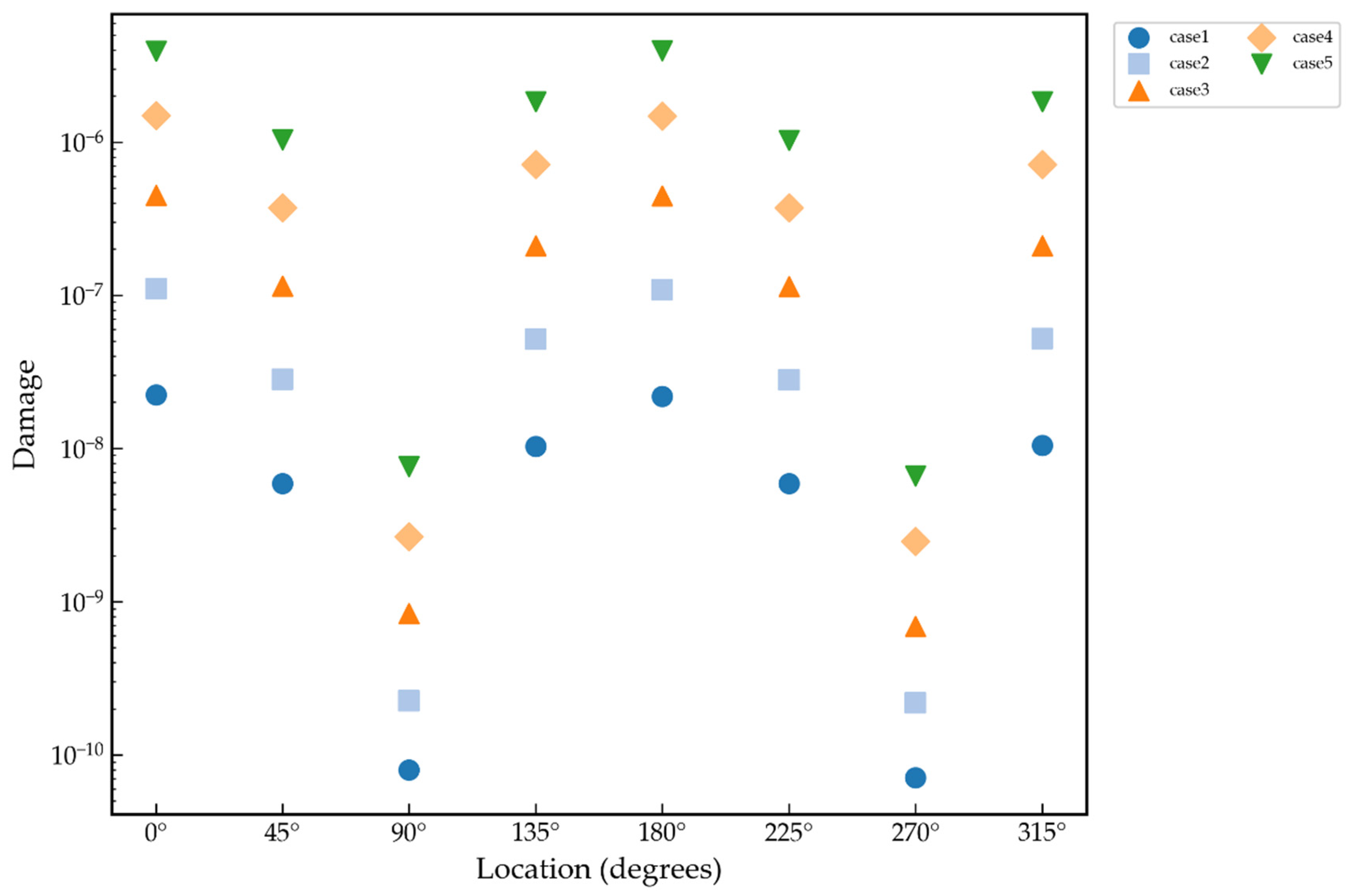
The GPR model is employed to estimate the short-term fatigue damage of the monopile foundation over a 600 s simulation period. As illustrated in Figure 18, the fatigue damage exhibits a pronounced circumferential variation, with maximum values occurring at the 0° and 180° positions. This is attributed to the fact that these directions are aligned with the primary bending plane of the structure, where the fore-aft bending moments reach their maximum and dominate fatigue damage accumulation. In contrast, the 90° and 270° positions are primarily subjected to weaker lateral loading, resulting in comparatively lower fatigue damage. Furthermore, for a given circumferential position, fatigue damage increases consistently with wind speed across different sea states, indicating the dominant role of aerodynamic loading in fatigue accumulation.

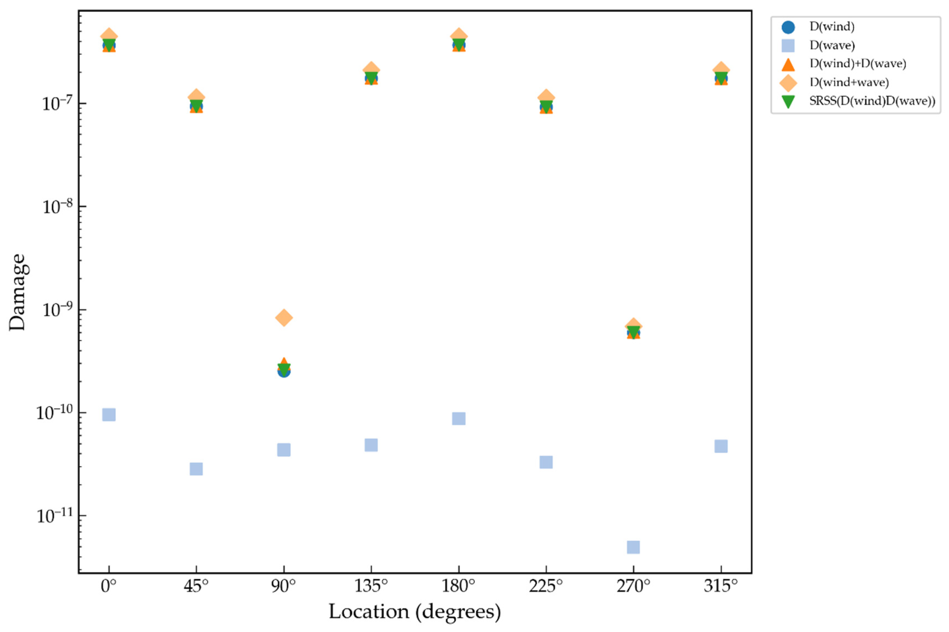
In conventional fatigue design of OWT, the amplification effects due to simultaneous wind and wave loads are often simplified or overlooked. To quantify this effect, fatigue damage is evaluated under three loading scenarios: wind-only, wave-only, and combined wind–wave loading. Two commonly used superposition methods, linear superposition and the square root of the sum of squares (SRSS), are adopted for comparison and defined as:

$$D=D_1+D_2,$$

(21)

$$D=\sqrt{{D_1}^2+{D_2}^2},$$

(22)

where D₁ and D₂ denote the damage induced by wind and wave loads, respectively, when applied independently.

The GPR model is used to estimate short-term fatigue damage under the most probable sea state (Case 3) over a duration of 600 s. As shown in Figure 19, wind-induced fatigue damage D(wind) significantly exceeds that caused by wave loading D(wave) at all circumferential positions. However, when comparing with fully coupled wind–wave simulations, both linear and SRSS approaches are found to systematically underestimate the total damage. This discrepancy highlights the strong nonlinear interaction between aerodynamic and hydrodynamic loads, which cannot be accurately captured by simple superposition assumptions.

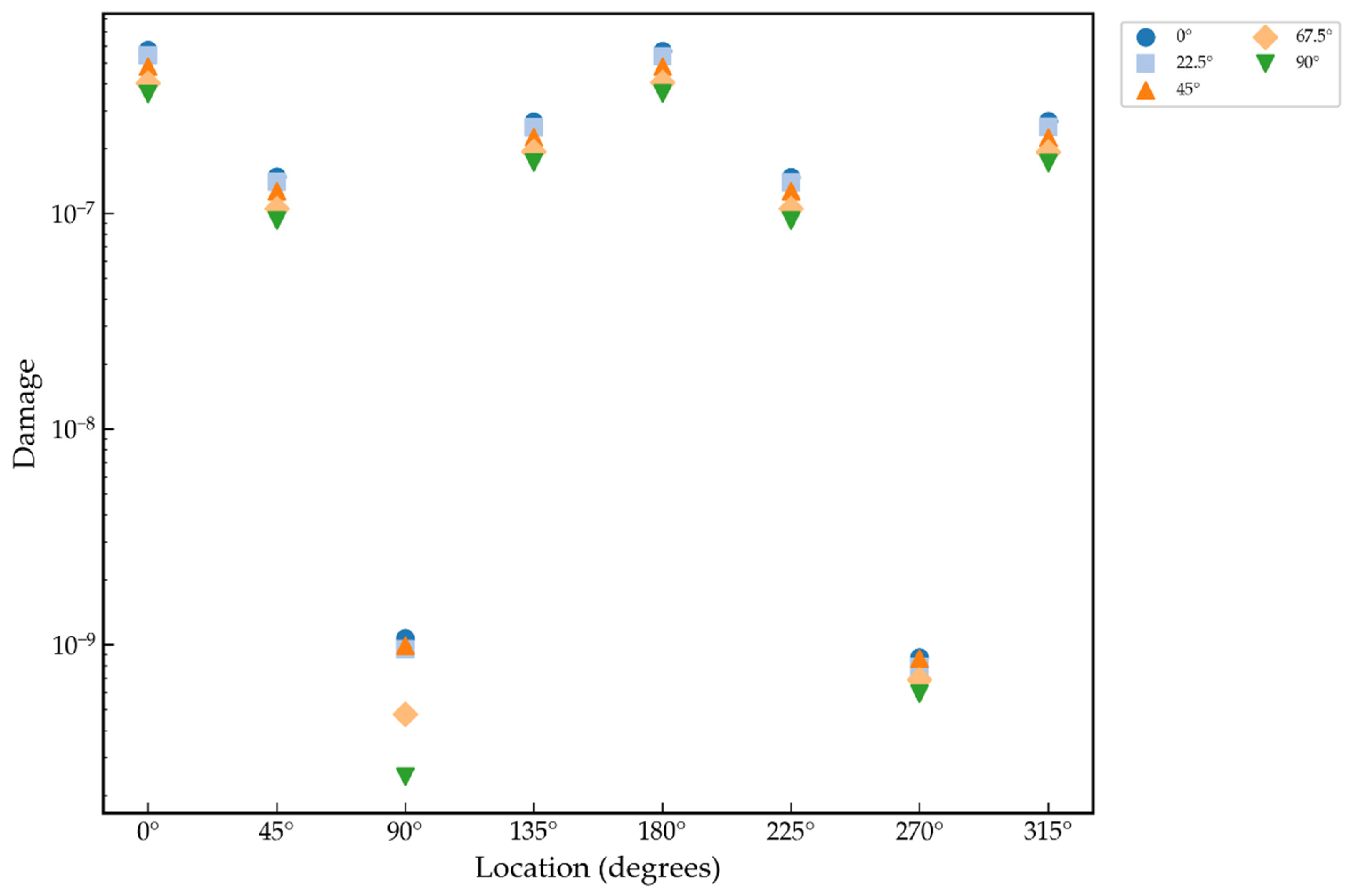
The impact of wind–wave directional misalignment is explored under Case 3 by changing the wave direction and keeping the wind direction unchanged. The resulting fatigue damage distributions at different circumferential positions are shown in Figure 20. It is observed that the overall damage patterns exhibit directional symmetry, with similar fatigue responses occurring at angle pairs such as (0°, 180°), (90°, 270°), and (45°, 225°). This symmetry arises from the structural geometry and the dominant loading direction of the wind. Since wind-induced loading governs the fatigue response and is fixed along the global X-axis, the variation in wave direction has a relatively limited influence on the global damage distribution pattern.

For a given wind–wave angle, the relative distribution of fatigue damage along the circumference remains consistent, with higher damage occurring at positions more closely aligned with the wind direction. Moreover, when examining a fixed circumferential position under varying wave directions, the fatigue damage is found to depend on the relative alignment between the wave propagation direction and the structural orientation. Specifically, smaller angles between the loading direction and the structural position lead to increased stress response and higher fatigue damage.

These results demonstrate that although wave direction has a secondary effect compared to wind loading, it can still influence local fatigue distribution through directional interaction. Therefore, accurate fatigue assessment of OWT foundations requires consideration of both wind–wave coupling and directional misalignment effects.

5. Conclusions

This study proposes an integrated fatigue assessment framework for OWT monopile foundations under combined wind–wave loading, combining a high-fidelity finite element model with surrogate modeling techniques. Based on the analysis, the following conclusions are reached:

(1)

The developed finite element model, incorporating soil–pile interaction via the p-y method, accurately reproduces structural dynamic and static responses, with deviations within acceptable engineering limits.

(2)

The surrogate-based framework significantly reduces computational cost by requiring only a limited number of simulations while maintaining high accuracy. Among the models, the Gaussian process model achieves the best performance, showing superior accuracy and robustness under small-sample conditions.

(3)

The proposed approach achieves great improvement in computational efficiency compared to direct simulations, with the GPR model yielding the highest accuracy, followed by SVR, while XGBoost and RF show relatively lower performance.

(4)

Fatigue damage is primarily governed by environmental loading: it increases with wind speed and significant wave height, but decreases with peak wave period. Wind loading dominates fatigue accumulation, whereas wave effects are secondary but non-negligible. Conventional load superposition methods (linear and SRSS) underestimate fatigue damage, confirming the importance of nonlinear wind–wave coupling effects. Fatigue damage exhibits pronounced circumferential non-uniformity, with maximum values occurring in the fore-aft directions due to dominant bending moments.

6. Limitations of the Dataset and Simulation Setup

It must be acknowledged that this study has several limitations, which will be discussed in detail below.

As discussed in Section 3, we simplify rotor aerodynamics to an equivalent thrust, tower wind load to static pressure, and waves to linear Airy theory. The fully coupled aero-hydro-servo-elastic response—including blade pitch control, tower shadow, dynamic wake, and nonlinear wave kinematics—is omitted, and future work should incorporate a fully coupled framework.

Further, fatigue damage is evaluated over 600 s of stabilized response, which corresponds to approximately 10 min. While this duration captures short-term variability, it does not represent the long-term statistical distribution of environmental conditions. Following IEC guidelines, longer simulations (1 h or more per sea state) would be needed to reduce sampling uncertainty, but this would dramatically increase computational cost. Our approach therefore provides a relative comparison rather than absolute long-term fatigue predictions.

Finally, although 60 samples are sufficient to train Gaussian Process Regression (GPR) with reasonable accuracy, they are inadequate for capturing highly nonlinear or extreme sea-state behaviors. Increasing the sample size to 180 or 300 improved the performance of tree-based models (XGBoost, RF) but did not further enhance GPR or SVR, indicating that GPR reaches its plateau with small datasets.

References

1. Ding, J.; Chen, H.; Liu, X.; Rashed, Y.F.; Fu, Z. Fatigue Reliability Analysis of Offshore Wind Turbines Under Combined Wind–Wave Excitation via Direct Probability Integral Method. J. Mar. Sci. Eng. 2025, 13, 506. [Google Scholar] [CrossRef]
2. McAuliffe, J.; Baisthakur, S.; Broderick, B.; Fitzgerald, B. Corrosion fatigue analysis of NREL’s 15-MW offshore wind turbine with time-varying stress concentration factors. J. Phys. Conf. Ser. 2024, 2767, 062023. [Google Scholar] [CrossRef]
3. Zhao, G.; Dong, S.; Zhao, Y. Fatigue reliability analysis of floating offshore wind turbines under the random environmental conditions based on surrogate model. Ocean Eng. 2024, 314, 119686. [Google Scholar] [CrossRef]
4. Gaidai, O.; Ashraf, A.; Cao, Y.; Sheng, J.; Zhu, Y.; Liu, Z. Lifetime assessment of semi-submersible wind turbines by Gaidai risk evaluation method. J. Mater. Sci. Mater. Eng. 2024, 19, 2. [Google Scholar] [CrossRef]
5. Zhu, X.; Cao, M.; Ostachowicz, W.; Xu, W. Damage Identification in Bridges by Processing Dynamic Responses to Moving Loads: Features and Evaluation. Sensors 2019, 19, 463. [Google Scholar] [CrossRef]
6. Fekhari, E.; Chabridon, V.; Muré, J.; Iooss, B. Given-data probabilistic fatigue assessment for offshore wind turbines using Bayesian quadrature. Data-Centric Eng. 2024, 5, e5. [Google Scholar] [CrossRef]
7. Liu, D.P.; Ferri, G.; Heo, T.; Marino, E.; Manuel, L. On long-term fatigue damage estimation for a floating offshore wind turbine using a surrogate model. Renew. Energy 2024, 225, 120238. [Google Scholar] [CrossRef]
8. Singh, D.; Haugen, E.; Laugesen, K.; Dwight, R.P.; Viré, A. Data-driven probabilistic surrogate model for floating wind turbine lifetime damage equivalent load prediction. Wind Energy Sci. 2025, 10, 2865–2888. [Google Scholar] [CrossRef]
9. Meng, D.; Yang, S.; Yang, H.; De Jesus, A.M.P.; Correia, J.; Zhu, S.-P. Intelligent-inspired framework for fatigue reliability evaluation of offshore wind turbine support structures under hybrid uncertainty. Ocean Eng. 2024, 307, 118213. [Google Scholar] [CrossRef]
10. Zhu, D.; Ding, Z.; Huang, X. Probabilistic model for fatigue damage estimation of wind turbines with hidden markov model and neural network. Ocean Eng. 2024, 310, 118663. [Google Scholar] [CrossRef]
11. Andrews, A.; Jain, R.K. Beyond Energy Efficiency: A clustering approach to embed demand flexibility into building energy benchmarking. Appl. Energy 2022, 327, 119989. [Google Scholar] [CrossRef]
12. Brooks, S.; Mahmood, M.; Roy, R.; Manolesos, M.; Salonitis, K. Self-reconfiguration simulations of turbines to reduce uneven farm degradation. Renew. Energy 2023, 206, 1301–1314. [Google Scholar] [CrossRef]
13. Delen, C.; Bal, S. A comprehensive experimental investigation of total drag and wave height of ONR Tumblehome, including uncertainty analysis. Ocean Eng. 2023, 284, 115232. [Google Scholar] [CrossRef]
14. Hu, Z.; Li, L.; Gao, X.; Xu, J.; Liu, X.; Gong, S.; Wang, W.; Shi, W.; Li, X. A Fully Coupled Sensitivity Analysis Framework for Offshore Wind Turbines Based on an XGBoost Surrogate Model and the Interpretation of SHAP. Sustainability 2025, 17, 9227. [Google Scholar] [CrossRef]
15. Wang, B.; Peng, L.; Huang, G.; Yang, X.; Liu, W.; Xin, Z. Research on fatigue load surrogate model for wind turbines considering wake effects. Acta Energiae Solaris Sin. 2025, 46, 623–628. [Google Scholar]
16. Herath, M.T.; Phillips, A.W.; John, N.S.; Brandner, P.; Pearce, B.; Prusty, G. Hydrodynamic response of a passive shape-adaptive composite hydrofoil. Mar. Struct. 2021, 80, 103084. [Google Scholar] [CrossRef]
17. Hu, X.; Gong, X.; Zhu, F.; Xing, X.; Li, Z.; Zhang, X. Thermal analysis and optimization of metal foam PCM-based heat sink for thermal management of electronic devices. Renew. Energy 2023, 212, 227–237. [Google Scholar] [CrossRef]
18. Feng, X.; Chen, J.; Liu, Z.; Zhang, Z.; Li, Y. Nonlinear effects on wave elevation of a focused water wave group. Appl. Ocean Res. 2025, 165, 104853. [Google Scholar] [CrossRef]
19. Shabarov, V.; Peplin, F.; Kalyasov, P.; Shaposhnikov, V. Analytical and numerical investigation of the lift system stability of the air cushion vehicle fitted with closed inflated side seals. Appl. Ocean Res. 2022, 120, 103045. [Google Scholar] [CrossRef]
20. Kumar, P.; Yadav, A.; Sardana, D.; Prasad, R. Rajni, Extreme wave height response to climate modes and its association with tropical cyclones over the Indo-Pacific Ocean. Ocean Eng. 2024, 296, 116789. [Google Scholar] [CrossRef]
21. Mittendorf, M.; Nielsen, U.D.; Bingham, H.B.; Storhaug, G. Sea state identification using machine learning—A comparative study based on in-service data from a container vessel. Mar. Struct. 2022, 85, 103274. [Google Scholar] [CrossRef]
22. Wang, W.; Yan, J.; Chen, S.; Liu, J.; Jin, F.; Wang, B. Gridded cemented riprap for scour protection around monopile in the marine environment. Ocean Eng. 2023, 272, 113876. [Google Scholar] [CrossRef]
23. Zheng, K.; Chen, B.; Yang, K.; Deng, Y.; Shi, J.; Zhou, G. Structural failure assessment system exemplified by dumbbell-shaped CFST arch. Eng. Struct. 2023, 284, 115987. [Google Scholar] [CrossRef]
24. Liu, F.; Lv, T.; Meng, Y.; Li, C.; Hou, X.; Xu, J.; Deng, X. Potential analysis of BESS and CCUS in the context of China’s carbon trading scheme toward the low-carbon electricity system. Renew. Energy 2023, 210, 462–471. [Google Scholar] [CrossRef]
25. Lv, H.-C.; Li, N.; Huang, X.-L.; Li, C.; Weng, C.-S. Signal characteristics and energy transmittance during detonation tube excitation in a gas–water–soil environment. Ocean Eng. 2024, 310, 118765. [Google Scholar] [CrossRef]
26. Li, T.; Yang, Q.; Zhang, X.; Ma, Y. Efficient fatigue damage estimation of offshore wind turbine foundation under wind-wave actions. J. Constr. Steel Res. 2024, 221, 108903. [Google Scholar] [CrossRef]
27. Yu, C.; Lv, X.; Huang, D.; Jiang, D. Reliability-based design optimization of offshore wind turbine support structures using RBF surrogate model. Front. Struct. Civ. Eng. 2023, 17, 1086–1099. [Google Scholar] [CrossRef]
28. Wang, L.; Kolios, A.; Liu, X.; Venetsanos, D.; Cai, R. Reliability of offshore wind turbine support structures: A state-of-the-art review. Renew. Sustain. Energy Rev. 2022, 161, 112250. [Google Scholar] [CrossRef]
29. Achmus, M.; Kuo, Y.-S.; Abdel-Rahman, K. Behavior of monopile foundations under cyclic lateral load. Comput. Geotech. 2009, 36, 725–735. [Google Scholar] [CrossRef]
30. Yang, Y.; Bashir, M.; Li, C.; Wang, J. Analysis of seismic behaviour of an offshore wind turbine with a flexible foundation. Ocean Eng. 2019, 178, 215–228. [Google Scholar] [CrossRef]
31. Shinozuka, M.; Jan, C.M. Digital simulation of random processes and its applications. J. Sound. Vib. 1972, 25, 111–128. [Google Scholar] [CrossRef]
32. IEC 61400-1:2019; Wind Energy Generation Systems—Part 1: Design Requirements. International Electrotechnical Commission: Geneva, Switzerland, 2019.
33. Wang, Y.; Leng, D.; Jin, J.; Li, Y.; Liu, G. Broadband vibration mitigation of offshore wind turbines using gradient metamaterial resonators. Ocean Eng. 2026, 354, 125035. [Google Scholar] [CrossRef]
34. Gentils, T.; Wang, L.; Kolios, A. Integrated structural optimisation of offshore wind turbine support structures based on finite element analysis and genetic algorithm. Appl. Energy 2017, 199, 187–204. [Google Scholar] [CrossRef]
35. McAuliffe, J.; Broderick, B.; Fitzgerald, B. A composite modelling approach for the fatigue analysis of offshore wind turbines considering corrosion-induced material degradation. Ocean Eng. 2026, 349, 123886. [Google Scholar] [CrossRef]
36. Peng, M.; Liu, M.; Gu, S.; Nie, S. Multiaxial Fatigue Analysis of Jacket-Type Offshore Wind Turbine Based on Multi-Scale Finite Element Model. Materials 2023, 16, 4383. [Google Scholar] [CrossRef]
37. Zhang, X.-L.; Zhang, B.-J.; Wang, D.; Xu, C.-S. Fatigue damage analysis method of offshore wind turbine foundation. Ocean Eng. 2024, 302, 117618. [Google Scholar] [CrossRef]
38. DNVGL-RP-C203; Fatigue Design of Offshore Steel Structures. DNV GL: Oslo, Norway, 2016.
39. Zhu, D.; Ding, Z.; Huang, X. Active learning model for probabilistic estimation of fatigue damage in wind turbines with latent variable uncertainty. Ocean Eng. 2025, 335, 121724. [Google Scholar] [CrossRef]
40. Chen, T.; Guestrin, C. XGBoost: A Scalable Tree Boosting System. In Proceedings of the 22nd ACM SIGKDD International Conference on Knowledge Discovery and Data Mining, San Francisco, CA, USA, 13–17 August 2016; Association for Computing Machinery: New York, NY, USA, 2016; pp. 785–794. [Google Scholar]
41. Youn, J.; Hwang, S.; Qian, X.; Im, S.; Son, S. A random forest-based method for reconstructing pressure fields in tropical cyclones from wind data. Atmos. Res. 2026, 330, 108588. [Google Scholar] [CrossRef]
42. Meshack, O.C.; Ohiri, P.C.; Mfonobong, E.B.; Ogomaka, C.C.; Anyalewechi, C.J. Integrating Multi-Resolution Remote Sensing Data for Daily Forest Fire Risk Forecasting in a Nigerian Savanna Ecosystem. World J. Adv. Eng. Technol. Sci. 2026, 18, 263–278. [Google Scholar] [CrossRef]
43. Belgiu, M.; Drăguţ, L. Random forest in remote sensing: A review of applications and future directions. ISPRS J. Photogramm. Remote Sens. 2016, 114, 24–31. [Google Scholar] [CrossRef]
44. Kaveh, N.; Ebrahimi, A.; Asadi, E. Comparative analysis of random forest, exploratory regression, and structural equation modeling for screening key environmental variables in evaluating rangeland above-ground biomass. Ecol. Inform. 2023, 77, 102251. [Google Scholar] [CrossRef]
45. Zhou, Z.; Qiu, C.; Zhang, Y. A comparative analysis of linear regression, neural networks and random forest regression for predicting air ozone employing soft sensor models. Sci. Rep. 2023, 13, 22420. [Google Scholar] [CrossRef]
46. Zhou, R.; Xu, Z.; Wang, H.; Liu, Y.; Nie, J. Flutter uncertainty analysis of flexible photovoltaic support structure considering stochastic aerodynamic and structural parameters. J. Wind. Eng. Ind. Aerodyn. 2026, 269, 106300. [Google Scholar] [CrossRef]
47. Flores-Lasluisa, J.X.; Huerta, F.; Cazorla-Amorós, D.; Morallón, E. Manganese oxides/LaMnO3 perovskite materials and their application in the oxygen reduction reaction. Energy 2022, 247, 123456. [Google Scholar] [CrossRef]
48. Smola, A.J.; Schölkopf, B. A tutorial on support vector regression. Stat. Comput. 2004, 14, 199–222. [Google Scholar] [CrossRef]
49. Pathirikattu, A.; Vakamalla, T.R. Exploration of machine learning models for hydrocyclone performance parameters prediction. Powder Technol. 2025, 465, 121355. [Google Scholar] [CrossRef]
50. Gao, Z.; Zhao, W. A data-driven approach for fatigue life of water intake risers. Mar. Struct. 2022, 83, 103188. [Google Scholar] [CrossRef]
51. Hofmann, M.; Steinke, F.; Scheel, V.; Charpiat, G.; Farquhar, J.; Aschoff, P.; Brady, M.; Schölkopf, B.; Pichler, B.J. MRI-Based Attenuation Correction for PET/MRI: A Novel Approach Combining Pattern Recognition and Atlas Registration. J. Nucl. Med. 2008, 49, 1875–1883. [Google Scholar] [CrossRef]
52. Fischer, T.; Vries, W.D.; Schmidt, B. Upwind Design Basis (WP4: Offshore Foundations and Support Structures); TU Delft: Delft, The Netherlands, 2010. [Google Scholar]
Figure 1. Structural arrangement of the 5 MW OWT and soil conditions.
Energies 19 02383 g001
Figure 2. FEM of pile–soil interaction using p-y springs.
Energies 19 02383 g002
Figure 3. The 3600 s time-history of maximum principal stress at the foundation mudline by OpenFAST.
Energies 19 02383 g003
Figure 4. The 3600 s time-history of maximum principal stress at the foundation mudline by FEM.
Energies 19 02383 g004
Figure 5. Definition of load directions applied to the OWT foundation.
Energies 19 02383 g005
Figure 6. Time history and power spectrum of the wind speed at the hub height.
Energies 19 02383 g006
Figure 7. (a) Time history, (b) power spectrum of wave elevation with Hs = 5 m, Tp = 10 s.
Energies 19 02383 g007
Figure 8. (a) Three-dimensional distribution and (b) two-dimensional distribution by LHS with Uhub, Tp, and Hs.
Energies 19 02383 g008
Figure 9. Methodology for fatigue damage assessment of OWT foundation.
Energies 19 02383 g009
Figure 10. Circumferential fatigue evaluation locations of the OWT foundation.
Energies 19 02383 g010
Figure 11. Fatigue damage prediction errors (MAPE and RE) for four models under 60 training samples.
Energies 19 02383 g011
Figure 12. Fatigue damage prediction errors (MAPE and RE) for four models under 180 training samples.
Energies 19 02383 g012
Figure 13. Fatigue damage prediction errors (MAPE and RE) for four models under 300 training samples.
Energies 19 02383 g013
Figure 14. Fatigue damage prediction errors R for (a) XGBoost, (b) RF, (c) SVR, and (d) GPR model under 60 training samples.
Energies 19 02383 g014
Figure 15. Fatigue damage prediction errors RMSE for (a) XGBoost, (b) RF, (c) SVR, and (d) GPR model under 60 training samples.
Energies 19 02383 g015
Figure 16. GPR predictions of fatigue damage with 95% prediction intervals.
Energies 19 02383 g016
Figure 17. Fatigue damage of OWT foundation with varied Uhub, Tp, and Hs.
Energies 19 02383 g017
Figure 18. Fatigue damage of OWT foundation under different sea states.
Energies 19 02383 g018
Figure 19. Fatigue damage of OWT foundation under different superposition methods.
Energies 19 02383 g019
Figure 20. Fatigue damage of OWT foundation under different wave incident angles.
Energies 19 02383 g020