Article

Adaptive ε-Constraint-Based Scheduling with Three-Network Verification and Closed-Loop Repair for Regional Integrated Energy Systems

1
School of Automation and Electrical Engineering, Lanzhou University of Technology, Lanzhou 730050, China
2
Huanxian Power Supply Company, State Grid Gansu Electric Power Company, Huanxian 745700, China
3
Xifeng District Power Supply Company, State Grid Gansu Electric Power Company, Xifeng 745000, China
*
Author to whom correspondence should be addressed.
Energies 2026, 19(10), 2381; https://doi.org/10.3390/en19102381
Submission received: 16 April 2026 / Revised: 9 May 2026 / Accepted: 12 May 2026 / Published: 15 May 2026
(This article belongs to the Section A: Sustainable Energy)

Abstract

Low-carbon scheduling of regional integrated energy systems (RIES) based only on energy-balance models may overlook the physical operating limits of distribution, gas, and heating networks, resulting in a gap between scheduling outcomes and actual operating boundaries. To address this issue, this paper proposes a framework integrating bi-objective scheduling, three-network posterior verification, and closed-loop repair. A mixed-integer linear programming model is first formulated with operating cost and carbon emissions as the two objectives, and an adaptive ε-constraint strategy is used to improve the characterization of the compromise region on the Pareto front. Posterior verification models are then established for the distribution, gas, and heating networks to assess the physical feasibility of representative solutions. When infeasibility is detected, a boundary-shrinking repair mechanism is triggered to iteratively update the scheduling boundaries. Case results show that the adaptive refined strategy improves the resolution of the compromise region by 3.2 times with only a 20.4% increase in computational time. Compared with the cost-optimal solution, the carbon-optimal solution reduces carbon emissions but increases peak purchased electricity from 7.333 MW to 11.1 MW, further tightening the lower-voltage margin of the distribution network. The results show that posterior physical verification and closed-loop repair provide additional support for evaluating and improving the engineering feasibility of RIES scheduling solutions.

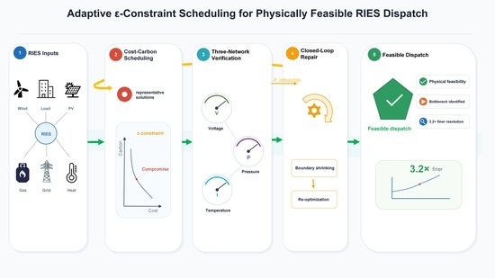
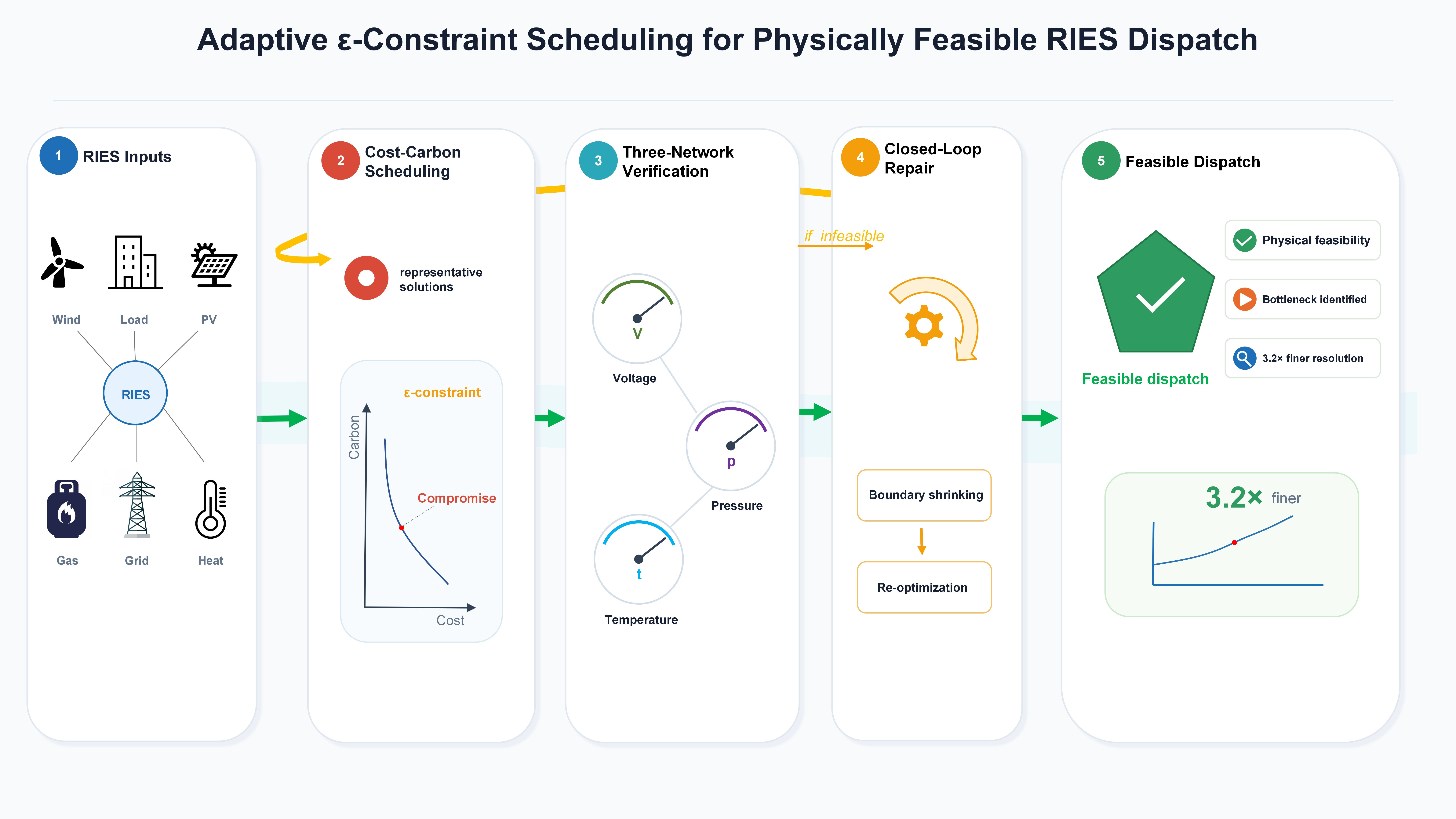
Graphical Abstract

1. Introduction

In recent years, under the continuous promotion of the “dual-carbon” goals, regional integrated energy systems (RIES) have attracted increasing attention as important carriers for low-carbon energy transition [1]. By coupling electricity, natural gas, heat, and cooling through coordinated conversion, storage, and supply devices, RIES can improve energy-utilization efficiency and provide operational flexibility for industrial parks, commercial districts, and residential communities [2,3].
Substantial progress has been made in the modeling and optimization of RIES. In terms of system representation, existing studies have developed electricity–heat coupling models considering thermal inertia [4], electricity–gas coupling models considering gas dynamic characteristics [5,6], and fully coupled multi-energy flow models integrating multiple energy carriers [7]. Graph-based methods [8], distributed modeling approaches [9], and multi-agent reinforcement learning frameworks [10] have also been introduced to improve representation accuracy, computational scalability, and coordination capability. Some studies have further incorporated physical network constraints into multi-energy flow optimization to better reflect actual operating conditions [11].
On the optimization side, exact approaches such as mixed-integer linear programming, second-order cone programming, and semidefinite programming have been widely used to handle complex operational constraints [12,13,14]. To address uncertainties in renewable generation, load demand, and energy prices, interval optimization, robust optimization, and stochastic programming have also been investigated [15,16,17]. In addition, approximate dynamic programming, deep reinforcement learning, and intelligent optimization algorithms have shown potential in alleviating dimensionality and improving real-time scheduling capability [18,19,20,21,22]. For multi-objective optimization in RIES and related multi-energy systems, ε-constraint formulations have been widely used to characterize trade-offs among economy, carbon emissions, and system security [23,24,25].
More recently, multi-objective optimization for complex energy and infrastructure systems has been extended toward hybrid evolutionary algorithms and learning-based paradigms [26,27,28], surrogate-assisted optimization [29], and quantum-inspired formulations [30,31]. These methods provide useful references for improving adaptivity, search efficiency, and representation flexibility in dynamic, uncertain, and high-dimensional decision spaces. However, the focus of this study is not to replace the optimization paradigm itself, but to improve the physical implementability of RIES scheduling solutions after optimization. When detailed distribution, gas, and heating network constraints are considered, model interpretability, constraint representation, and engineering feasibility remain critical issues. Therefore, the ε-constraint method is adopted in this study as a transparent and interpretable Pareto-front construction tool, rather than as a fundamentally new optimization algorithm. This structure allows representative scheduling solutions to be naturally connected with posterior physical verification and closed-loop repair.
Despite the above advances, the physical implementability of scheduling results still requires further attention. Many scheduling models are mainly established based on energy-balance relationships and device-level operating constraints. Although effective for system-level dispatch, such models do not necessarily guarantee that the obtained solutions remain physically feasible when mapped to distribution, gas, and heating networks. A scheduling-layer feasible solution may still cause voltage violations, pressure-limit tightening, or temperature-related risks at the physical network layer [32,33,34,35,36]. Although some studies have incorporated network constraints, reliability assessment, or physical feasibility checks, many remain at the stage of posterior assessment. Once infeasibility or insufficient margin is identified, a unified mechanism for feeding verification results back to the scheduling layer and forming a closed-loop correction process is still relatively lacking.
This issue is particularly important for RIES operation. As the system shifts among cost-oriented, carbon-oriented, and compromise-oriented dispatch, the underlying supply pattern may change accordingly. For example, a lower-carbon solution may reduce local gas-fired generation and increase dependence on external electricity purchase, thereby transferring part of the operational pressure to the grid side. Variations in gas utilization and heat supply allocation may also alter gas-network pressure and heating-network temperature margins. Therefore, the trade-off among economy, carbon reduction, and operational security cannot be adequately understood only from scheduling-layer objective values; the physical response of coupled networks must also be examined.
For multi-objective scheduling, the compromise region of the Pareto front is particularly important because it contains candidate solutions with balanced economic and environmental performance. However, conventional uniform ε-scanning may not simultaneously achieve satisfactory computational efficiency and sufficient local resolution in this region. Therefore, this paper improves the local characterization of the compromise region within the ε-constraint framework and further connects representative solutions with three-network physical verification and feedback repair.
To address these problems, this paper proposes an integrated framework for RIES that combines bi-objective scheduling, three-network posterior verification, and closed-loop repair. First, a mixed-integer linear programming scheduling model is developed with operating cost and carbon emissions as the two objectives, and a coarse-plus-refined ε-constraint scanning strategy is adopted to improve the characterization of the compromise region. Second, posterior verification models are established for the distribution, gas, and heating networks to assess the network-level feasibility of representative scheduling solutions. Third, when infeasibility or insufficient margin is identified, the verification results are fed back to the scheduling layer through a boundary-shrinking repair mechanism, forming a closed-loop process of “optimal scheduling–three-network verification–feedback repair.” In this way, the physical consistency and engineering implementability of scheduling results can be improved without directly embedding all nonlinear network models into the upper-level scheduling optimization.
Based on a typical-day case study of a northern China industrial park, this paper analyzes the trade-off relationships among operating cost, carbon emissions, and network risk under different scheduling tendencies. In addition, an effective carbon emission intensity (ECI) index is introduced to explain the carbon-attribution characteristics of gas-turbine-based generation under combined cooling, heating, and power operation, helping interpret the mechanism behind the observed cost–carbon trade-off.
The main contributions of this paper are summarized as follows.
(1)
A bi-objective MILP scheduling model for RIES is developed with operating cost and carbon emissions as the optimization objectives. Within the established ε-constraint framework, a normalized compromise metric is used to identify the local refined region, and a coarse-plus-refined scanning strategy is adopted to improve the characterization of the compromise region and provide representative scheduling solutions for subsequent physical verification.
(2)
Posterior verification models are established for the distribution, gas, and heating networks, and a boundary-shrinking closed-loop repair mechanism is designed to improve the physical feasibility and engineering implementability of scheduling solutions.
(3)
Based on a typical-day case study, the trade-off relationships among cost, carbon emissions, and network risk are analyzed, and the dominant network bottleneck and critical periods under different scheduling tendencies are identified. In addition, the ECI index is introduced to support the interpretation of emission-reduction mechanisms under different operating strategies.
The remainder of this paper is organized as follows. Section 2 introduces the system description and scheduling assumptions. Section 3 presents the bi-objective scheduling model and the adaptive ε-constraint strategy. Section 4 describes the three-network posterior verification and closed-loop repair method. Section 5 provides the case study and discussion. Finally, Section 6 concludes the paper.

2. System Description and Scheduling Assumptions

2.1. RIES Architecture and Energy Coupling Relationships

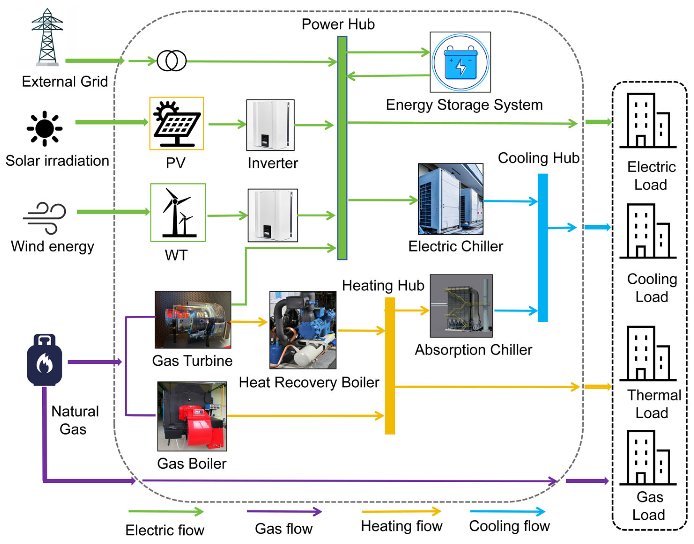
As illustrated in Figure 1, the core coupling chain of the proposed system can be summarized as natural gas–gas turbine–electricity/heat–cooling. In this structure, the energy storage system and the utility grid provide operational flexibility on the electricity side, while the gas boiler serves as a supplementary heat source on the thermal side. This coupling structure indicates that operating cost, carbon emissions, and network security do not evolve independently, but are mutually coupled through the multi-energy conversion chain.

2.2. Scheduling Assumptions

The scheduling horizon is set to 24 h with a time step of 1 h. In this study, a typical-day hourly scheduling framework is adopted to jointly optimize electric, heating, and cooling loads together with renewable energy output.
(1)
Rigid load satisfaction without load shedding
P s h e d , t = H s h e d , t = L s h e d , t = G s h e d , t = 0 , t T
Equation (1) indicates that electricity, heating, and cooling demands are all treated as rigid loads throughout the scheduling horizon, and the model does not permit load shedding as a means of restoring feasibility. Natural gas consumption is determined endogenously by the operating states of the devices, and no interruptible gas load is explicitly considered.
(2)
Renewable curtailment is allowed with penalty costs
Curtailment of wind power and photovoltaic generation is allowed, and the corresponding penalty cost is incorporated into the objective function, as detailed in Section 3.2.

3. Bi-Objective Scheduling Model

This section develops a bi-objective MILP scheduling model for RIES, in which operating cost and carbon emissions are taken as the two optimization objectives. Based on this model, the ε-constraint method is adopted to generate the Pareto front, and the resolution of the compromise region is further improved through adaptive scanning.

3.1. Objective Functions

3.1.1. Operating Cost Objective

The operating cost consists of electricity purchasing and selling, natural gas purchasing, demand charges, and renewable-curtailment penalties, and can be expressed as
min C = t T c e , t P b u y , t + c g , t V g a s , t + λ c u r t P c u r t , t t + c p e a k P p e a k 1000
Equation (2) represents the daily operating cost of the system, including electricity purchasing cost, natural gas purchasing cost, demand charges, and renewable-curtailment penalty cost. Since P p e a k is measured in MW while the demand charge is charged in kW, the factor 1000 is introduced to ensure unit consistency.

3.1.2. Carbon Emission Objective

The total carbon emissions consist of emissions from electricity purchasing and natural gas consumption, which can be written as
min E = t T μ e P b u y , t + μ g G t o t a l , t t
Equation (3) represents the total daily carbon emissions of the system, which are composed of emissions associated with purchased electricity and natural gas consumption. This is also a common accounting approach in integrated energy system studies [36].

3.1.3. Definition of Effective Carbon Emission Intensity (ECI)

In this case study, the power-generation efficiency of the gas turbine is η e = 0.26 If the total natural gas consumption of the gas turbine was entirely allocated to electricity generation, the corresponding carbon emission intensity would reach 1.72 tCO2/MWh, which is much higher than that of the utility grid (0.7035). However, under the combined cooling, heating, and power operating mode, the gas turbine generates electricity while simultaneously providing high-grade waste heat. Therefore, the effective carbon emission intensity of gas-turbine power generation at time period t, denoted by e E C I , t , is defined as follows:
E C I G T = μ g G G T , t μ g H h r b , t η g b P g t , t
Equation (4) defines the effective carbon emission intensity of gas-turbine power generation. The first term in the numerator represents the direct carbon emissions associated with the natural gas consumed by the gas turbine, while the second term represents the equivalent avoided carbon emissions due to waste-heat recovery, which can offset the heat supply otherwise provided by the gas boiler. The denominator is the gas-turbine electricity output. Therefore, ECI reflects the net attributed carbon emissions per unit of electricity generation under the combined heat and power condition, rather than the original combustion-based emission intensity of the gas turbine itself.
Under the present parameter setting, the effective carbon emission intensity of the gas turbine can be reduced from 1.72 kg/kWh to approximately 0.512 kg/kWh. When the recovered waste heat is fully utilized, e E C I , t can further decrease to about 0.48 tCO2/MWh, indicating that gas-turbine-based generation can exhibit certain emission-reduction potential when the recovered heat is effectively utilized.
It should be noted that ECI is used as an interpretive carbon-attribution index rather than an additional optimization objective or constraint. The carbon-emission objective in Equation (3) still follows the standard purchased-electricity plus natural-gas accounting form, while ECI is introduced to explain the emission-reduction mechanism of gas-turbine-based CCHP operation.

3.2. Constraint Conditions

3.2.1. Grid Interaction Constraints

To avoid physically meaningless arbitrage caused by frequent switching between electricity purchasing and selling under the time-of-use tariff mechanism, binary variables are introduced to enforce mutual exclusiveness between the two actions within the same time period.
(1)
Mutual exclusiveness between electricity purchasing and selling
0 P b u y , t P g r i d , max μ b u y , t 0 P s e l l , t P g r i d , max μ s e l l , t μ b u y , t + μ s e l l , t 1 μ b u y , t , μ s e l l , t 0 , 1
(2)
Capacity limits and peak-period purchasing limit
P b u y , t μ g r i d , t P g r i d , max P s e l l , t 1 μ g r i d , t P g r i d , max P b u y , t P p e a k , max , t T p e a k
(3)
Definition of peak demand
P p e a k P b u y , t t T , P p e a k 0
Equations (5)–(7) describe the mutual exclusiveness between electricity purchasing and selling, the upper limits of grid-interactive trading power, and the definition of the maximum demand during the scheduling horizon, respectively. Here, μ b u y , t and μ s e l l , t are binary variables indicating the electricity purchasing and selling states, respectively; μ g r i d , t is a time-period indicator used to distinguish the peak-period purchasing limit; and P g r i d , max and P p e a k , max denote the overall grid-interaction capacity limit and the peak-period purchasing limit, respectively. The numerical values of the grid-interaction limits are listed in Appendix A.

3.2.2. Renewable Generation and Curtailment Constraints

The available photovoltaic and wind power in each time period is allocated between actual utilization and curtailment, as defined below.
P p v , t + P p v , c u r t , t = P p v , a v a , t P ω t , t + P ω t , c u r t , t = P ω t , a v a , t
Equation (8) describes the allocation of the forecast available photovoltaic and wind power output between actual utilization and curtailed energy.
0 P p v , t P p v , a v a , t 0 P ω t , t P ω t , a v a , t P p v , c u r t , t , P ω t , c u r t , t 0
Equation (9) gives the non-negativity and upper-bound constraints for the actual photovoltaic and wind power outputs as well as the curtailed power. Here, P p v , c u r t , t and P ω , c u r t , t denote the curtailed photovoltaic and wind power at time period t , respectively, and their sum corresponds to the total renewable curtailment used in the cost objective. The curtailment penalty coefficient used in the objective function is given in Appendix A.

3.2.3. Device Models and Coupling Constraints

(1)
Natural gas consumption and output limit of the gas turbine
G G T , t = P g t , t η e , g t , 0 P g t , t P g t max , t T
(2)
Waste-heat recovery and output limit
H h r b , t = P g t , t η h r b , 0 H h r b , t H h r b max , t T
(3)
Heat output of the gas boiler and natural-gas conversion
H g b , t = G G B , t η g b , G t o t a l , t = G G T , t + G G B , t , V g a s , t = G t o t a l , t L H V g a s , t T
(4)
Energy conversion relationships and capacity limits of cooling devices
L a c , t = C O P a c H a c , i n , t , 0 L a c , t L a c max , t T
L e c , t = C O P e c P e c , i n , t , 0 P e c , i n , t P e c , i n max , t T
(5)
Ramp-rate constraint of the gas turbine
R a m p G T P g t , t P g t , t 1 R a m p G T , t T
(6)
Output bounds of the gas boiler
H g b , min μ g b , t H g b , t H g b , max u g b , t , μ g b , t 0 , 1
Equations (10)–(16) describe the multi-energy coupling relationships, capacity limits, and operating constraints of the gas turbine, waste-heat recovery unit, gas boiler, and cooling devices. Specifically, Equation (10) defines the natural-gas consumption and rated output limit of the gas turbine; Equation (11) describes waste-heat recovery and its upper output limit; Equation (12) gives the gas-boiler heat output, the total natural-gas energy consumption, and the conversion between natural-gas energy and volume; Equations (13) and (14) characterize the energy-conversion relationships and capacity limits of the absorption chiller and electric chiller; Equation (15) imposes the ramp-rate constraint of the gas turbine; and Equation (16) gives the operating-state-dependent output bounds of the gas boiler. Here, P g t max , H h r b max , L a c max , P e c , i n max , H g b min , H g b max , and L H V g a s are the rated capacity and energy-conversion parameters listed in Appendix A. To preserve linearity, the recovered waste heat is approximated as a linear function of gas-turbine power output.

3.2.4. Multi-Energy Balance Constraints

Electricity balance
P b u y , t + P g t , t + P p v , t + P ω t , t + P d i s , t = P l o a d , t + P c h , t + P s e l l , t + P e c , i n , t
Heat balance
H h r b , t + H g b , t = H l o a d , t + H a c , i n , t
Cooling balance
L a c , t + L e c , t = L l o a d , t
Equations (17)–(19) represent the electricity, heating, and cooling energy balance constraints of the system in each time period, respectively. Here, H a c , i n , t denotes the thermal input to the absorption chiller, and P e c , i n , t denotes the electric input to the electric chiller.

3.2.5. Energy Storage Constraints

SOC dynamics
S O C t + 1 = S O C t + η c h P c h , t t E b a t P d i s , t t η d i s E b a t
SOC bounds and cyclical consistency
S O C ¯ S O C t S O C ¯ S O C 1 = S O C T + 1
Charging/discharging power limits
0 P c h , t c P ¯ c h μ c h , t 0 P d i s , t P ¯ d i s μ d i s , t
Mutual exclusiveness between charging and discharging
μ c h , t + μ d i s , t 1 μ c h , t , μ d i s , t 0 , 1
Equations (20)–(23) describe the dynamic evolution of the state of charge, the SOC bounds, the charging/discharging power limits, and the mutual exclusiveness between charging and discharging, respectively. Here, E b a t is the rated energy capacity of the energy storage system; η c h and η d i s are the charging and discharging efficiencies; P c h max and P d i s max are the charging and discharging power limits; and μ c h , t and μ d i s , t are binary variables representing the charging and discharging states of the energy storage system. The corresponding numerical values are listed in Appendix A.

3.2.6. ε-Constraint Formulation

In the ε-constraint method, the carbon-emission objective is converted into a constraint [25]:
min C s . t . E ε
Equation (24) transforms the original bi-objective optimization problem into a single-objective problem that minimizes operating cost subject to an upper bound on carbon emissions. By scanning different values of ε, the Pareto front between operating cost and carbon emissions can be obtained.

3.3. Adaptive ε-Constraint Scanning and Compromise-Solution Identification

An adaptive ε-constraint scanning strategy is adopted in this study to identify the compromise solution on the Pareto front. The procedure is summarized as follows.
(1)
Extreme-point solution
The cost-optimal solution (Opt-Cost) and the carbon-optimal solution (Opt-Carbon) are first obtained, yielding the carbon-emission range E min , E max .
(2)
Coarse scan
A set of N c uniformly distributed ε values is selected over E min , E max , and the MILP model is solved point by point to obtain the coarse Pareto front.
(3)
Compromise metric and compromise-region identification
The operating cost and carbon emissions are first normalized as
C ^ = C C min C max C min , E ^ = E E min E max E min
Equation (25) performs dimensionless normalization of operating cost and carbon emissions, thereby eliminating the influence of differences in units and magnitudes between the two objectives.
The compromise metric, defined as the Euclidean distance to the ideal point, is given by
J = C ^ 2 + E ^ 2
Equation (26) defines the Euclidean distance to the ideal point and uses it as the compromise indicator J . The coarse-scan solution with the minimum value of J is selected as the compromise-solution candidate. If the index of this candidate is denoted by i , the refined interval is selected from the adjacent coarse ε levels around this point, i.e., [ ε i 1 , ε i + 1 ] for an interior candidate. If the candidate lies at the boundary of the coarse scan, the nearest available adjacent interval is used instead.
Therefore, the refined region is not manually specified, but is automatically determined by the normalized compromise metric.
(4)
Refined scan and merging
A refined scan is then performed by densely sampling N f ε values within the selected local interval. The resulting refined Pareto points are merged with the coarse-scan results, and duplicate points are removed to form the final Pareto front.
This coarse-plus-refined procedure is not specific to the case study. It only requires the objective values obtained from an initial coarse ε-constraint scan and a normalized compromise metric. Therefore, it can be transferred to other bi-objective scheduling problems where the local compromise region needs higher-resolution characterization. If decision-maker preferences differ, the Euclidean distance in Equation (26) can also be replaced by a weighted or preference-based metric.
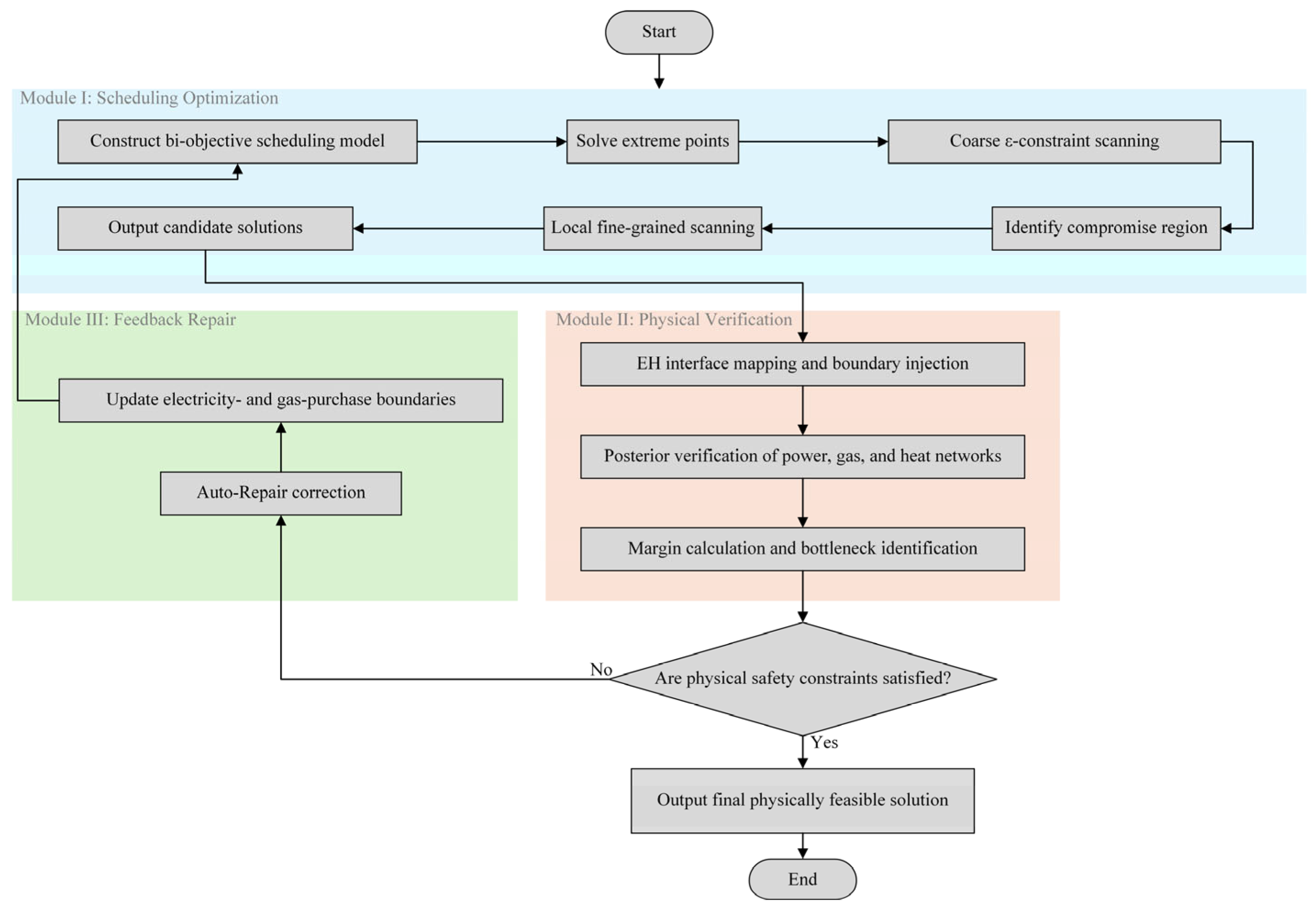
As illustrated in Figure 2, the overall workflow of the proposed method proceeds from scheduling optimization to physical verification and then to feedback repair, forming a closed-loop analysis framework of optimization–verification–repair.

4. Three-Network Posterior Verification and Closed-Loop Repair Method

Since park-level scheduling models are usually built on energy-balance relationships and simplified device characteristics, their solutions may lead to voltage violations or pipeline pressure distortions when implemented in actual physical networks. To address this issue, this paper establishes a closed-loop framework of scheduling, verification, and repair. Candidate scheduling solutions are first generated by the MILP model in the scheduling layer and then mapped to the adopted standard benchmark networks as boundary conditions for posterior verification. Specifically, the candidate solutions are examined using the nonlinear verification models of the IEEE 33-bus distribution network, the 14-node gas network, and the 17-node heating network. If physical bottlenecks are identified, the Auto-Repair mechanism shrinks the electricity-purchasing and gas-purchasing boundaries and re-solves the scheduling model until the voltage, pressure, and temperature margins all satisfy the required safety limits. As illustrated in Figure 2, this process forms a closed-loop workflow of optimization, verification, and feedback repair.

4.1. Energy Hub Interface Mapping and Spatiotemporal Alignment

To connect the scheduling layer in Section 3 with the physical-network verification layer in Section 4.2, Section 4.3 and Section 4.4, an energy-hub interface mapping model based on a coupling matrix is established. This model converts the system-level energy decision variables obtained from the scheduling layer into boundary injection conditions at the access nodes of the distribution, gas, and heating networks, as expressed by
P 25 , t I n j G 3 , t L o a d G 13 , t L o a d T 15 , t s = η t r 1 / η t r 0 0 0 0 0 1 0 0 0 0 0 1 0 0 0 0 0 1 P t , E b u y P t , E s e l l G t , G T G t , G B T s e t , t
In Equation (27), the left-hand side represents the nodal injection or equivalent load quantities in the distribution, gas, and heating networks, while the right-hand side contains the scheduling variables obtained from the optimization model in Section 3. The intermediate matrix describes the cross-network coupling relationships associated with EH1 and EH2. Here, η t r denotes transformer efficiency.
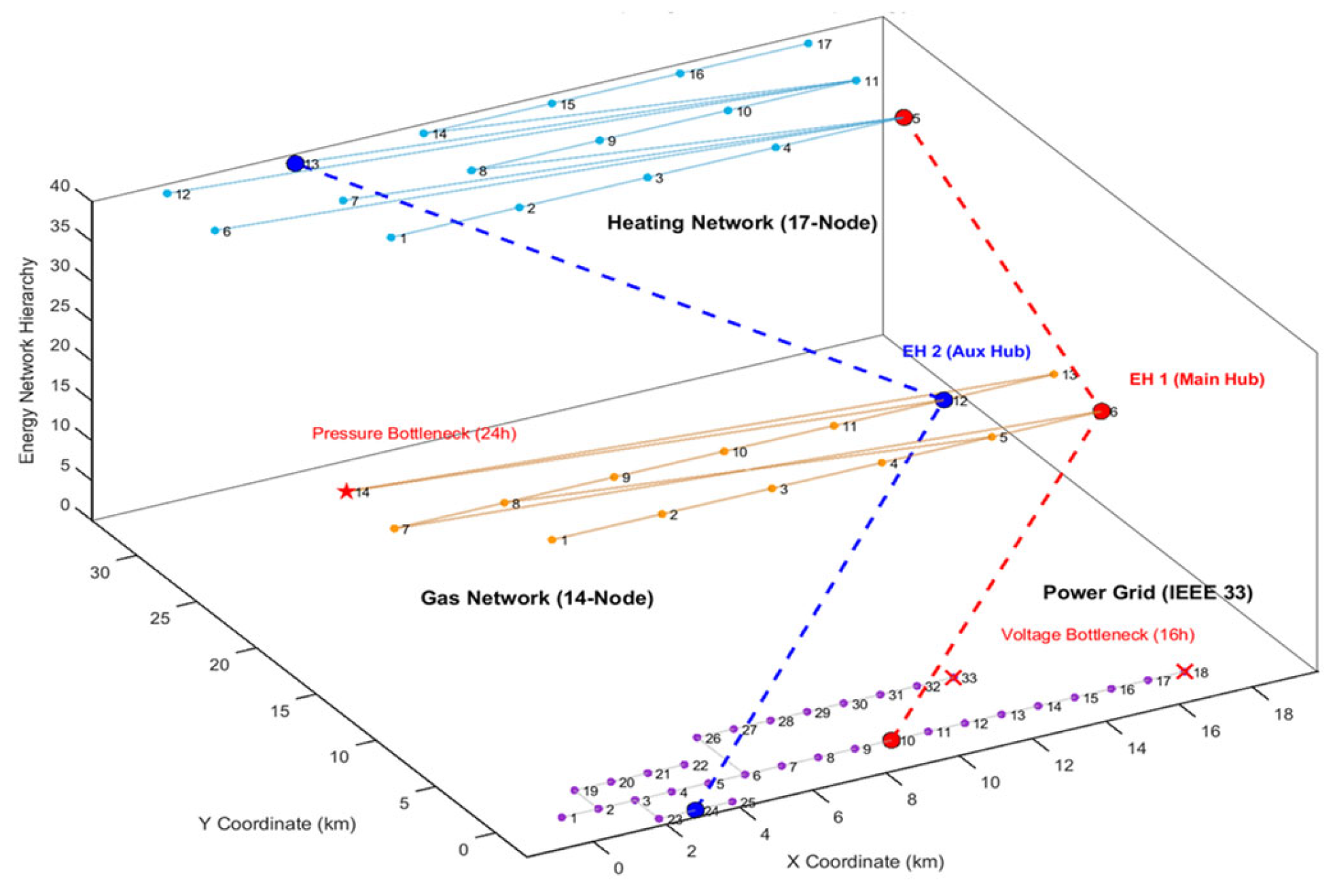
Through this mapping, the scheduling-layer results are converted into unified nodal boundary injections for the subsequent DistFlow, Weymouth, and thermo-hydraulic verification models. The hierarchical coupling topology of the energy system is illustrated in Figure 3.

4.2. Posterior Verification Model of the Distribution Network

The posterior verification of the distribution network is based on the DistFlow power-flow model, which has been widely applied in distribution network operation analysis and coupled energy-network modeling [37,38].
p j = P i r i j l i j P l o a d , j + P g e n , j Q j = Q i x i j l i j Q l o a d , j + Q g e n , j V j 2 = V i 2 2 r i j P i j + x i j Q i j + r i j 2 + x i j 2 l i j l i j = P i j 2 + Q i j 2 V i j 2
Equation (28) gives the DistFlow relationships of the distribution network, including nodal active/reactive power balance, branch voltage drop, and the coupling relationship associated with the squared branch current term.

4.3. Posterior Verification Model of the Gas Network

The posterior verification of the gas network is described using the steady-state pipeline-flow relationship and the nodal gas-flow balance equation.
F m n F m n = K m n 2 f m 2 f n 2
F i n F o u t = S n L n
Equations (29) and (30) represent the steady-state Weymouth flow relationship of gas pipelines and the nodal flow-balance equation of the gas network, respectively. Owing to the nonconvex nature of this model, its tractability in multi-energy network modeling has attracted considerable attention in the literature [39,40].

4.4. Posterior Verification Model of the Heating Network

4.4.1. Hydraulic Balance Equations

A steady-state hydraulic model is adopted for the heating network to describe the relationship among mass flow rate, nodal pressure, and branch pressure drop.
(1)
Nodal mass conservation
j A i m ˙ i j = m ˙ l o a d , i m ˙ s o u r c e , i
(2)
Branch pressure-drop equation
β i j = K h , i j m ˙ i j m ˙ i j
Equations (31) and (32) represent the nodal mass conservation relationship and the branch pressure-drop equation of the heating network, respectively. Here, A i denotes the set of branches connected to node i , and K h , i j is the pipe resistance coefficient.

4.4.2. Thermal Balance Equations

The thermal model describes heat exchange during circulation and the heat loss along the pipeline.
(1)
Load heat-exchange equation
H l o a d , i = m ˙ i C p ( T s , i T r , i )
(2)
Temperature attenuation equation
T e n d = T a m b + ( T s t a r t T a m b ) e λ L m ˙ C p
Equations (33) and (34) describe the nodal heat-exchange relationship and the temperature attenuation caused by pipeline heat loss, respectively. Here, C p is the specific heat capacity of water, T a m b is the ambient temperature, and L i j is the pipe length.
By combining graph-based topology with physical governing equations, the hydraulic balance, temperature distribution, and heat-loss characteristics of the district heating network can be represented with higher fidelity [41,42]. The hierarchical coupling network topology of the integrated energy system is shown in Figure 3.

4.5. Margin Indices and Bottleneck Identification

To quantify the distance between the operating state and the corresponding physical boundary, three margin indices are defined for voltage, pressure, and temperature constraints.
V m arg i n , t = min i N V i , t V min V max V min
p m arg i n , t = min j M f j , t f min f max f min
T m arg i n , t = min i H T s , i ( t ) T s , min T s , max T s , min , T s , max T s , i ( t ) T r , max T r , min
Equations (35)–(37) define the voltage margin of the distribution network, the pressure margin of the gas network, and the temperature margin of the heating network, respectively. All three indices are constructed from the distance between the operating state and the corresponding safety boundary. A smaller margin indicates that the corresponding network is closer to its physical bottleneck.

4.6. Closed-Loop Repair Strategy

To account for the possible mismatch between the dispatch-layer solution and the benchmark physical networks used for posterior verification, a closed-loop repair strategy is adopted. After the representative scheduling solution is obtained, it is mapped to the electricity, gas, and heating networks for posterior verification. If any network-layer constraint is violated, the corresponding outer-layer boundary is updated and the scheduling model is re-solved until all networks pass verification or the maximum repair iteration number is reached.
For power-network verification, the dispatch-layer electric demand is mapped to the benchmark feeder through a network-scale coefficient S v e r , as expressed in Equation (38). In this study, S v e r = 0.18 is adopted as the calibrated baseline setting, while S v e r = 0.16 and S v e r = 0.17 are used only for sensitivity analysis in Section 5.6.
P v e r , l o a d , t = S v e r P l o a d , t + P e c , i n , t + P c h , t P d i s , t
Equation (38) maps the dispatch-layer electric demand to the benchmark distribution-network load for posterior verification. Here, P v e r , l o a d , t is the mapped verification load, P e c , i n , t is the electric input power of the electric chiller, and P c h , t and P d i s , t are the charging and discharging powers of the energy storage system, respectively.
If posterior verification fails at iteration k, the electricity-purchasing and gas-purchasing boundaries are updated according to Equations (39) and (40), where Ω P ( k ) and Ω G ( k ) denote the violated time sets identified by the power and gas networks, respectively. The shrinking factor η r e p controls the repair intensity. In the main case, η r e p = 0.90 is used as the baseline value, while η r e p = 0.85 and η r e p = 0.95 are compared in Section 5.6.
P ¯ b u y , t ( k + 1 ) = η r e p P ¯ b u y , t ( k ) t Ω P ( k ) P ¯ b u y , t ( k ) t Ω P ( k )
G ¯ b u y , t ( k + 1 ) = η r e p G ¯ b u y , t ( k ) t Ω G ( k ) G ¯ b u y , t ( k ) t Ω G ( k )
Equations (39) and (40) update the upper bounds of electricity purchasing and natural gas purchasing, respectively. Here, P ¯ b u y , t ( k ) and G ¯ b u y , t ( k ) denote the purchasing upper bounds at repair iteration k , while Ω P k and Ω G k denote the violated time sets identified by power- and gas-network posterior verification, respectively.
The proposed Auto-Repair mechanism is a feasibility-restoration layer rather than a globally exact reformulation of the fully coupled nonlinear network-constrained scheduling problem. This decoupled design avoids embedding distribution-power-flow, gas-flow, and thermo-hydraulic constraints directly into the MILP scheduling model, but may introduce a certain loss of optimality because the feasible region is progressively tightened according to posterior verification results. Therefore, the repair process aims to improve physical implementability rather than to guarantee the global optimum of a fully integrated formulation.
F P ( k ) = F G ( k ) = F H ( k ) = 1 o r k = K r e p max
Equation (41) gives the stopping criterion of the repair loop F p ( k ) , F G ( k ) , and F H ( k ) are binary verification flags for the power, gas, and heating networks at iteration k , respectively, where a value of 1 indicates that the corresponding network passes posterior verification. The repair process stops when all three networks pass posterior verification or when k reaches K r e p max . In this study, K r e p max = 6 is adopted as the formal maximum number of repair iterations.
The method does not claim unconditional convergence under arbitrary stressed conditions; instead, its empirical convergence and parameter sensitivity are examined in Section 5.6. In the studied case, the heating-network temperature margins remain positive and the gas network does not trigger posterior infeasibility; therefore, active repair is mainly driven by the distribution-network voltage violation. For operating conditions with heating-network violations, the same feedback-repair logic can be extended by adjusting heat-source temperature or thermal boundary settings.

5. Case Study and Results Discussion

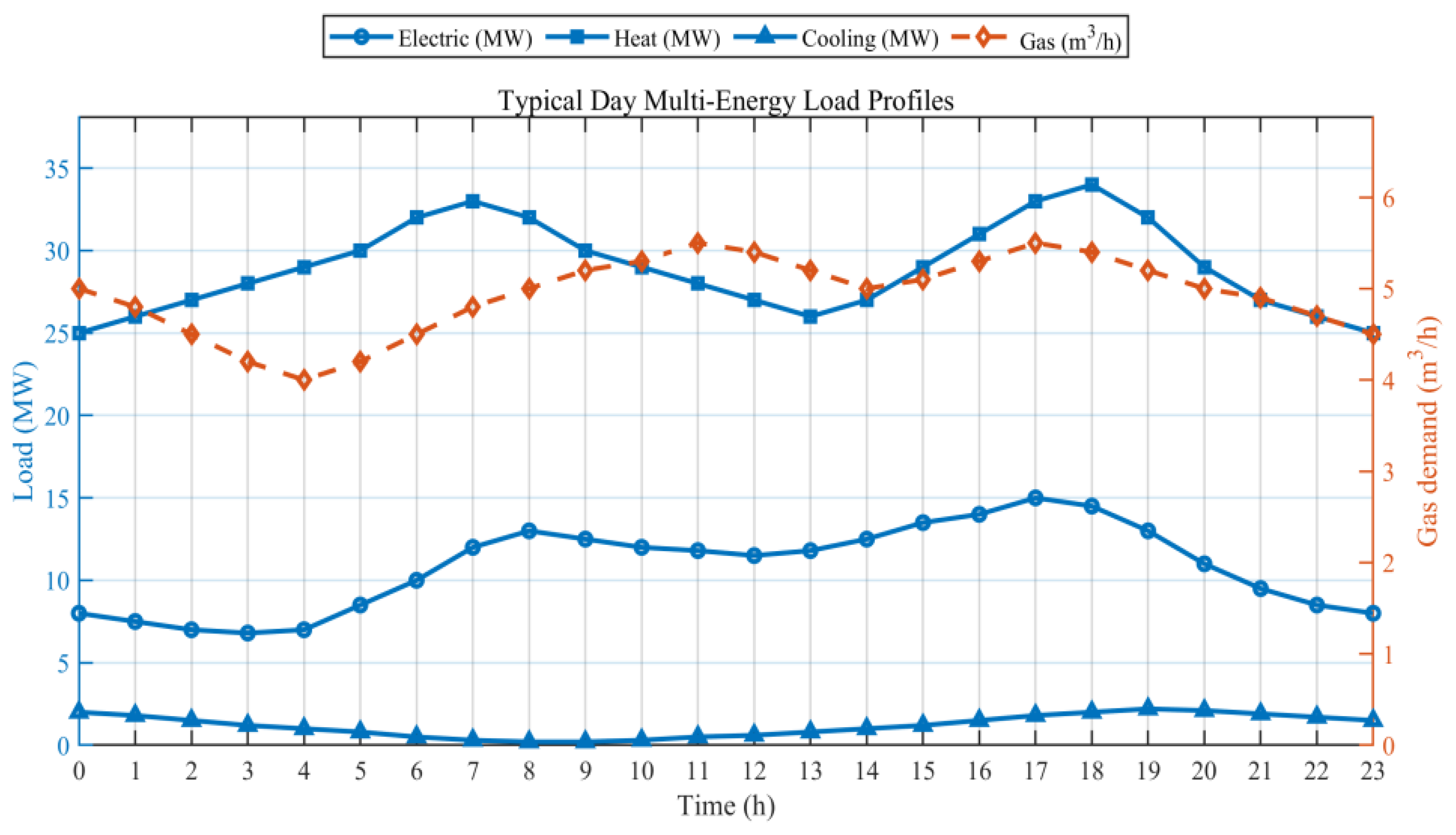
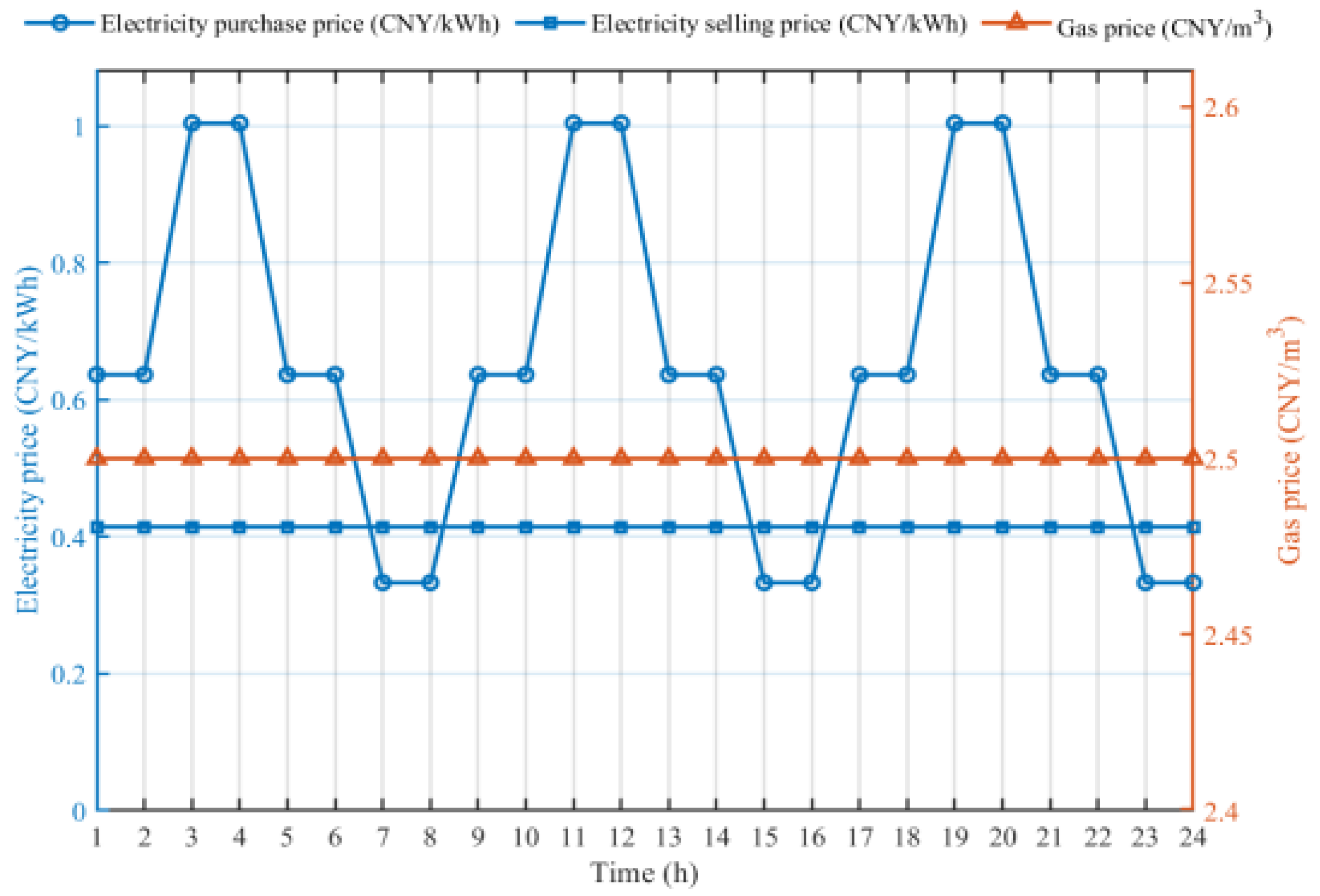
This study considers a typical-day operating scenario of an industrial park in northern China. The typical daily electricity, heating, and cooling load profiles, together with the electricity and natural gas price curves, are shown in Figure 4 and Figure 5. The detailed device parameters are given in Appendix A, the key settings for posterior verification and feedback repair are summarized in Appendix B, and the complete network data and implementation details are provided in the Supplementary Materials.

5.1. Scenario and Parameter Settings

5.1.1. Physical Network Mapping

To verify the physical feasibility of the scheduling solutions, a scenario-mapping approach is adopted to map the park-level energy-flow configuration onto standard test networks. In this framework, the typical-day data of the industrial park are used for the scheduling layer, while the standard benchmark networks are used for posterior feasibility screening. The network topology and coupling relationships are illustrated in Figure 3, and the interface correspondence is listed in Table 1. Considering voltage and pressure sensitivity, terminal nodes of the IEEE 33-bus distribution network are selected for distribution-network access verification, while for the gas network, one node close to the main gas source and another pressure-sensitive terminal node are chosen to characterize pressure-gradient variations.

5.1.2. Device and Evaluation Parameters

The parameters related to capacity, efficiency, ramp-rate limits, carbon-emission factors, and energy prices are used consistently in the scheduling, posterior verification, and sensitivity-analysis stages, and their values are listed in Appendix A.

5.2. Comparative Strategies and Evaluation Metrics

5.2.1. Two Baseline Strategies

Two baseline strategies are introduced for comparison under the same modeling framework.
(1)
Baseline-Price (price-driven):
The on/off status and output of each device are determined according to the time-of-use electricity price and device efficiencies, while satisfying the load demand and the same grid-interaction and device constraints as those used in the main model.
(2)
Baseline-Smooth (grid-smoothing):
Under the same operational constraints as the main model, this strategy takes the minimization of the peak purchased electricity power P p e a k during the scheduling horizon as the primary objective, thereby obtaining a feasible scheduling solution that tends to suppress the peak pressure imposed on the power grid.

5.2.2. Evaluation Metrics

The two baseline strategies are introduced to represent typical operational tendencies rather than competing optimization algorithms. The methodological comparison is conducted between the conventional uniformly coarse ε-constraint scan and the proposed coarse-plus-refined ε-constraint strategy, as further discussed in Section 5.3.2. The evaluation metrics include operating cost, carbon emissions, peak purchased electricity power, and the compromise indicator defined by Equation (26).

5.3. Multi-Objective Optimization Results and Pareto Front

5.3.1. Characteristics of the Pareto Front

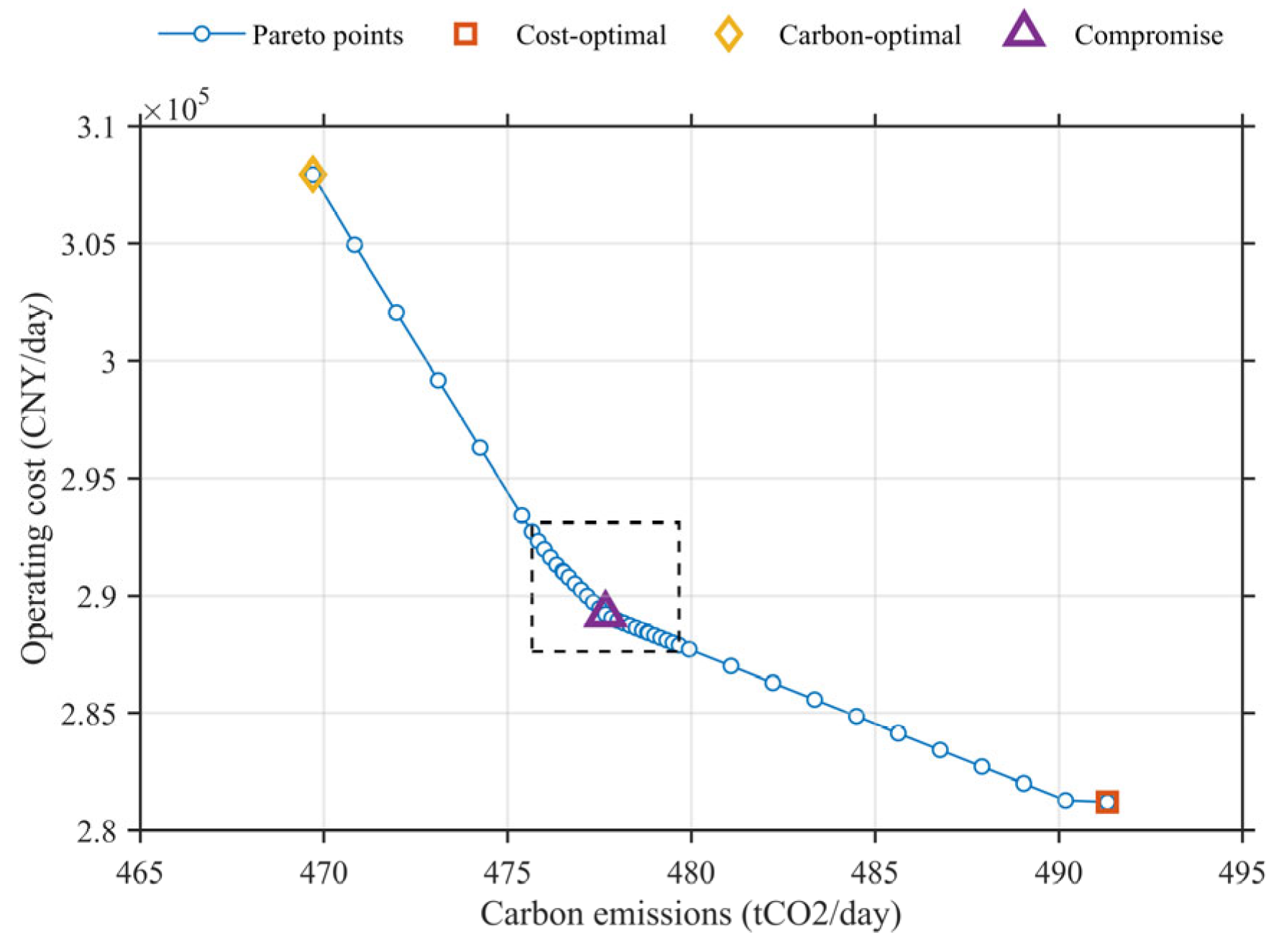
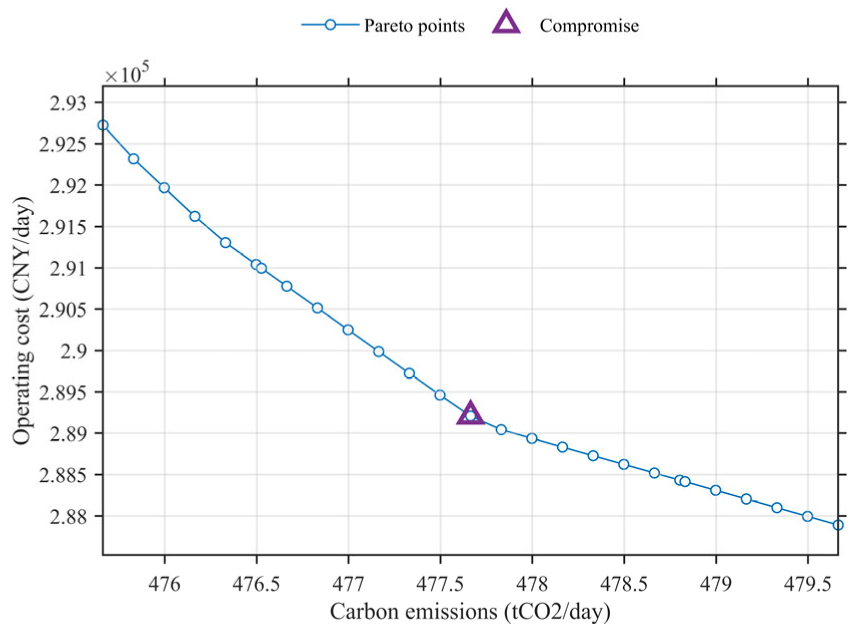
The Pareto front is generated using the adaptive ε-constraint scanning strategy. Specifically, the coarse scan contains 20 sampling points and the refined scan contains 25 sampling points, resulting in a total of 45 candidate solutions. After merging and removing duplicate points, 44 distinct Pareto solutions are obtained, denoted as the solution set P. The Pareto front and the locally refined compromise region are shown in Figure 6 and Figure 7, respectively.
Table 2 reports the operating cost, carbon emissions, and peak purchased electricity power of the representative solutions. It can be observed that, as the system gradually shifts from the cost-optimal solution toward the carbon-optimal solution, the share of local gas-fired generation decreases while the dependence on external electricity purchasing increases, leading to a higher peak purchased power. This indicates that the emission-reduction pathway is not achieved simply by lowering total energy consumption; instead, part of the operational pressure is transferred to the grid side through energy substitution. Its physical implications will be further discussed in Section 5.5.

5.3.2. Efficiency Analysis of the Adaptive Scanning Strategy

To improve the solution resolution in the compromise region, this paper adopts an adaptive ε-constraint strategy combining a coarse scan with local refined scanning. The coarse scan is first used to identify the overall shape of the Pareto front, and then additional points are inserted around the compromise region to obtain a more stable local boundary. Table 3 compares the performance of this strategy with that of the conventional uniformly coarse ε-constraint strategy.
As shown in Table 3, compared with the conventional coarse ε-constraint method, the proposed coarse-plus-refined strategy improves the resolution of the compromise region by 3.2 times while increasing the computational burden by only 20.4%. This demonstrates that local refinement can significantly improve the characterization quality of the compromise region at a relatively small additional computational cost, thereby enhancing the reliability of compromise-solution identification.

5.3.3. Trade-Off Between Carbon Reduction and Peak Purchased Electricity

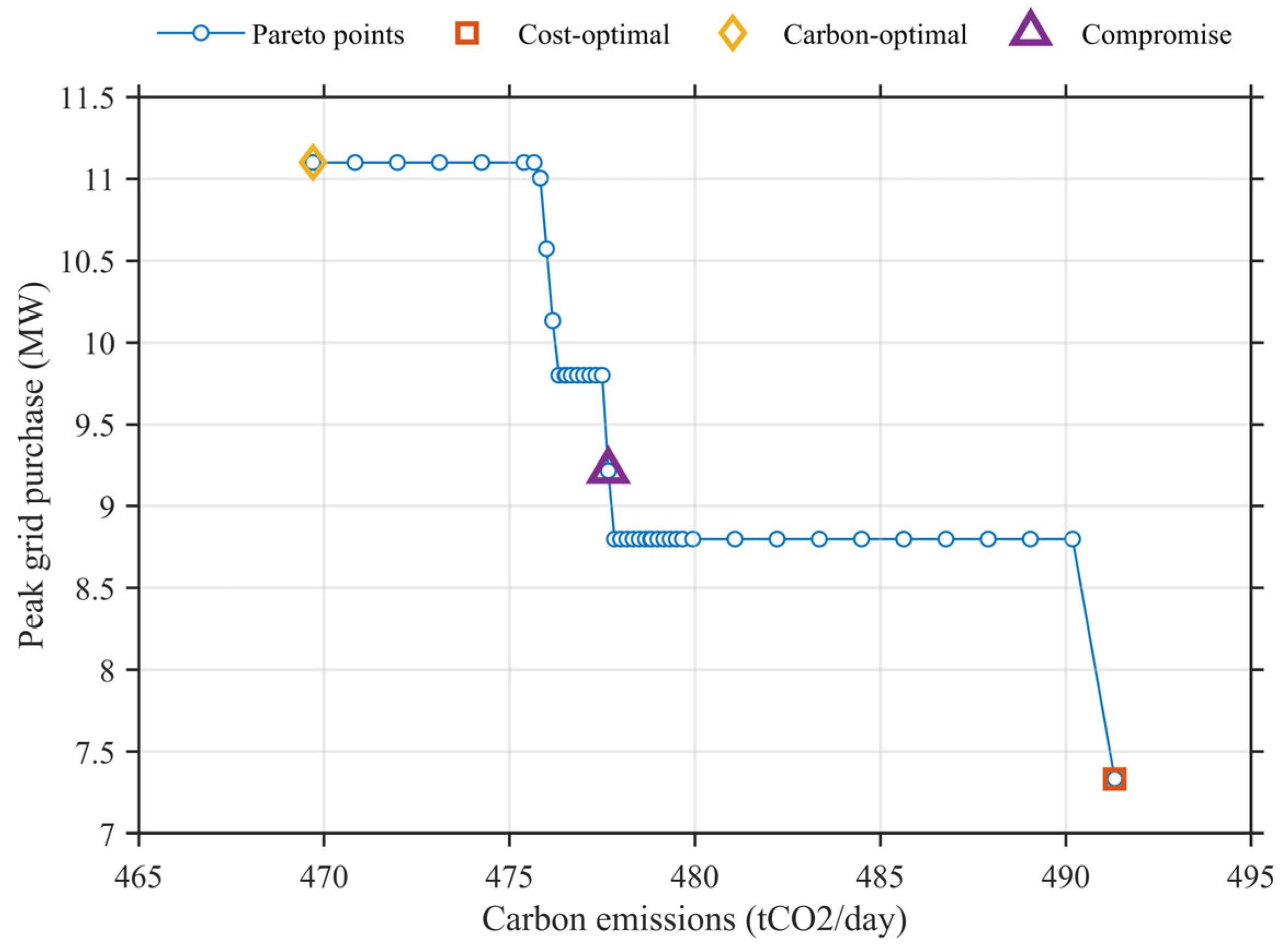
Figure 8 shows that peak purchased electricity generally increases as the scheduling solution moves from the cost-optimal end toward the carbon-optimal end of the Pareto set. Compared with the cost-optimal solution, the carbon-optimal solution increases peak purchased electricity from 7.333 MW to 11.1 MW, corresponding to a 51.4% increase. This indicates that aggressive carbon reduction may substantially intensify peak stress on the distribution network.
The step-like variation of peak purchased electricity is mainly caused by the definition of the indicator itself, since it is determined by the maximum hourly electricity purchase within the day. When the operating state crosses certain carbon-emission thresholds, the peak purchased electricity may change abruptly rather than continuously. From the ECI perspective in Section 3.1.3, when the recovered waste heat of the gas turbine is not sufficiently utilized, the marginal emission-reduction advantage of local gas-fired generation weakens, and the model becomes more inclined to use external grid electricity.
The compromise solution lies between the two extreme solutions and restrains the expansion of peak purchased electricity while still achieving considerable emission reduction. Therefore, it provides a more balanced trade-off among economic performance, carbon reduction, and grid-side security.

5.4. Strategy Comparison and Discussion

5.4.1. Comparison Between Baseline and Optimized Strategies

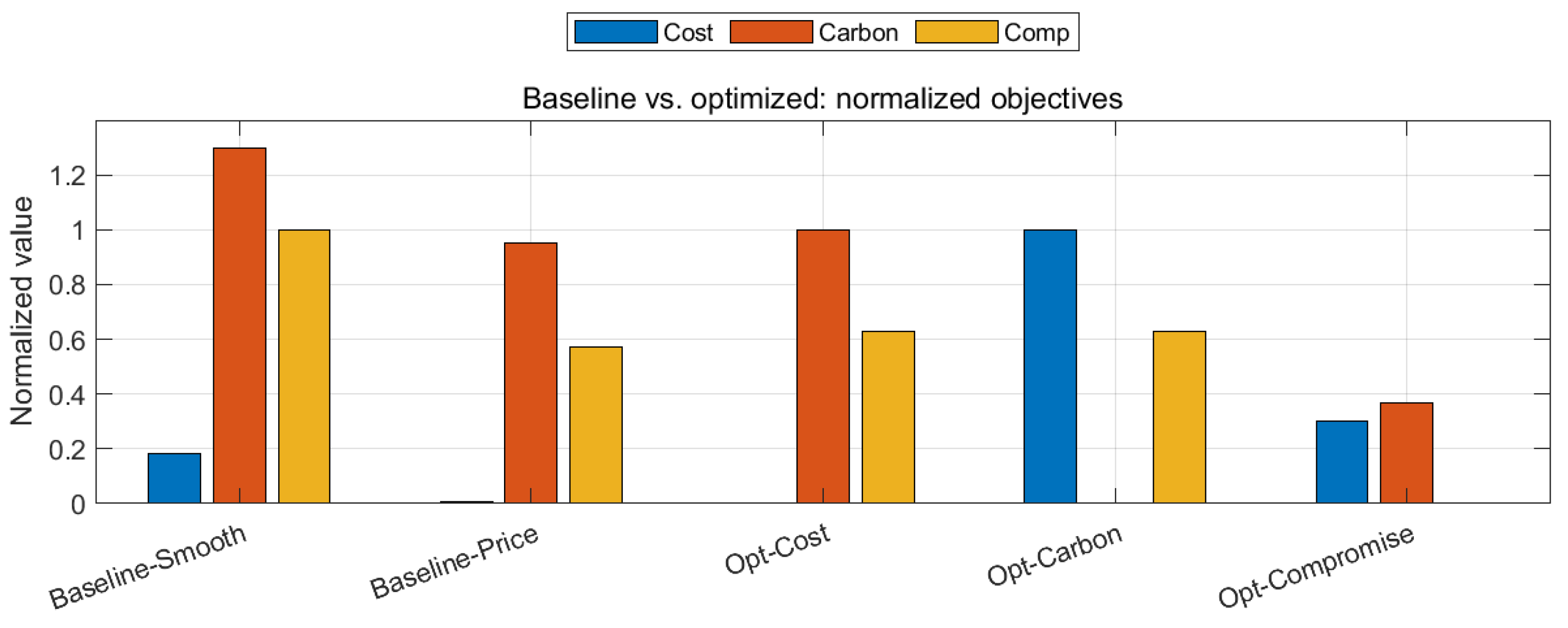
Under the unified assumption of rigid load satisfaction (Shed = 0), two baseline strategies and three representative optimized solutions are compared. As shown in Figure 9, Baseline-Smooth achieves the smoothest purchased-electricity profile but incurs a pronounced carbon penalty, whereas Opt-Compromise provides a more balanced performance in the compromise region of the Pareto front.
Compared with Baseline-Price, Opt-Compromise reduces carbon emissions by approximately 2.57% (490.26 → 477.66 t), increases operating cost by approximately 2.76% (281,454 → 289,208 CNY), and decreases peak purchased electricity by approximately 10.5% (10.3 → 9.216 MW), indicating a more balanced trade-off among economy, carbon reduction, and grid-side security.

5.4.2. Operating Characteristics of the Baseline-Smooth Strategy

The Baseline-Smooth strategy represents an extreme grid-smoothing operating mode. Under this strategy, peak purchased electricity is close to 0.00 MW because the objective strongly suppresses grid exchange. However, maintaining internal energy balance requires sustained gas-turbine output, resulting in the highest daily carbon emissions among all compared strategies. This result indicates that grid-side smoothing alone may reduce external electricity dependence but can sacrifice economic and environmental performance. By contrast, the proposed multi-objective framework provides a more balanced use of grid interaction and local energy conversion.

5.4.3. 24-H Multi-Energy Balance Under the Compromise Solution

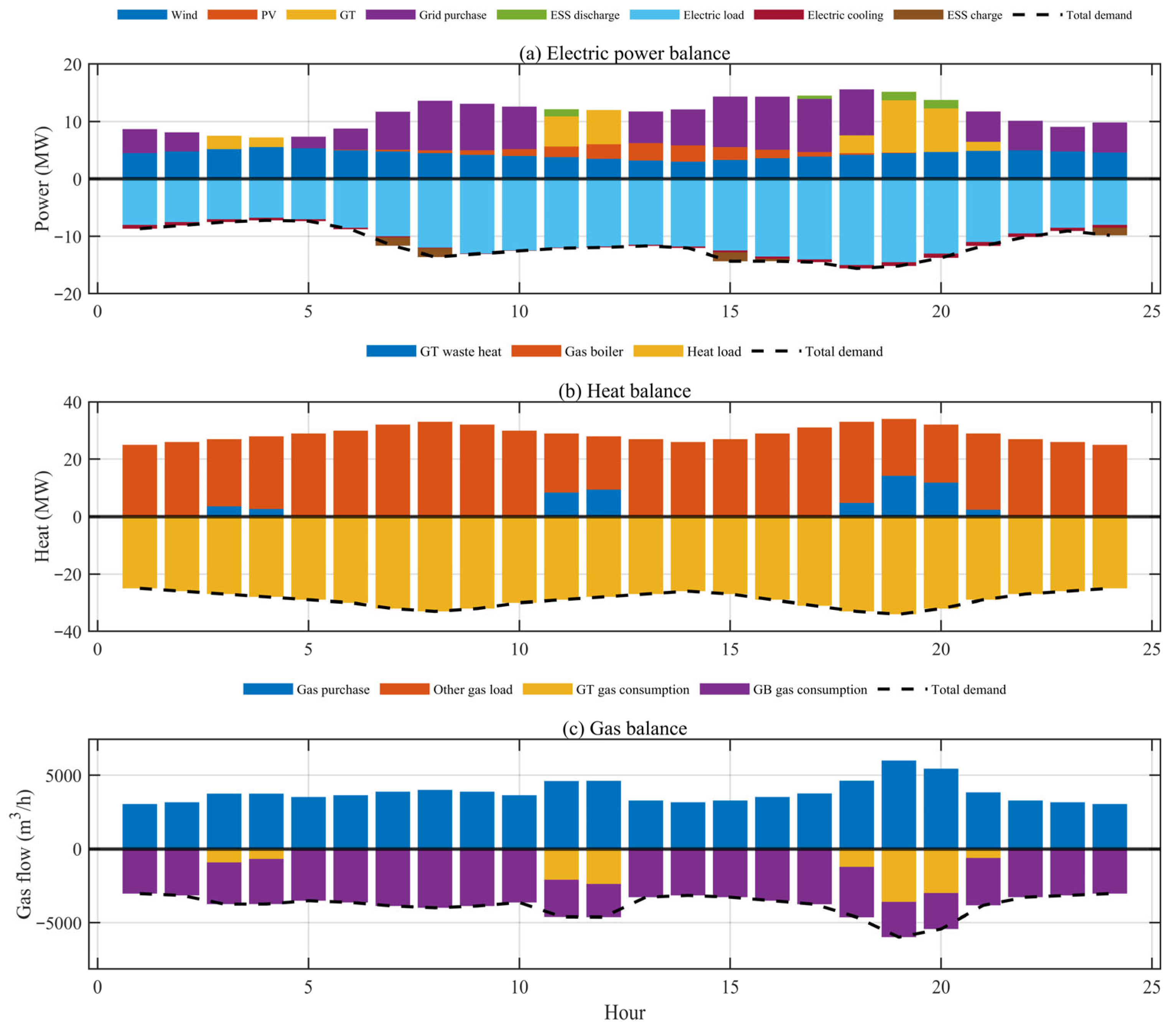
As shown in Figure 10, the compromise solution satisfies the electricity, gas, and heat demands throughout the 24 h horizon under the rigid-load assumption. The electricity supply is jointly provided by grid purchase, renewable generation, gas-turbine output, and battery discharge, while battery charging and electric cooling consume part of the available power. The gas demand is mainly allocated to the gas turbine and gas boiler, with the external base gas load acting as a background component. The heat demand is primarily met by recovered waste heat and gas-boiler output. Overall, the compromise solution exhibits a balanced multi-energy dispatch pattern and provides a time-domain interpretation of the posterior network-margin variation discussed in Section 5.5.

5.5. Three-Network Posterior Verification Results and Bottleneck Analysis

The representative solutions are further examined by calibrated posterior verification over the electricity, gas, and heating networks. Because the scheduling layer does not explicitly embed the physical network constraints, the initial solutions may violate the benchmark-network limits in some periods. Closed-loop repair is then applied to restore implementable solutions whenever possible.

5.5.1. Overall Calibrated Posterior-Verification Results

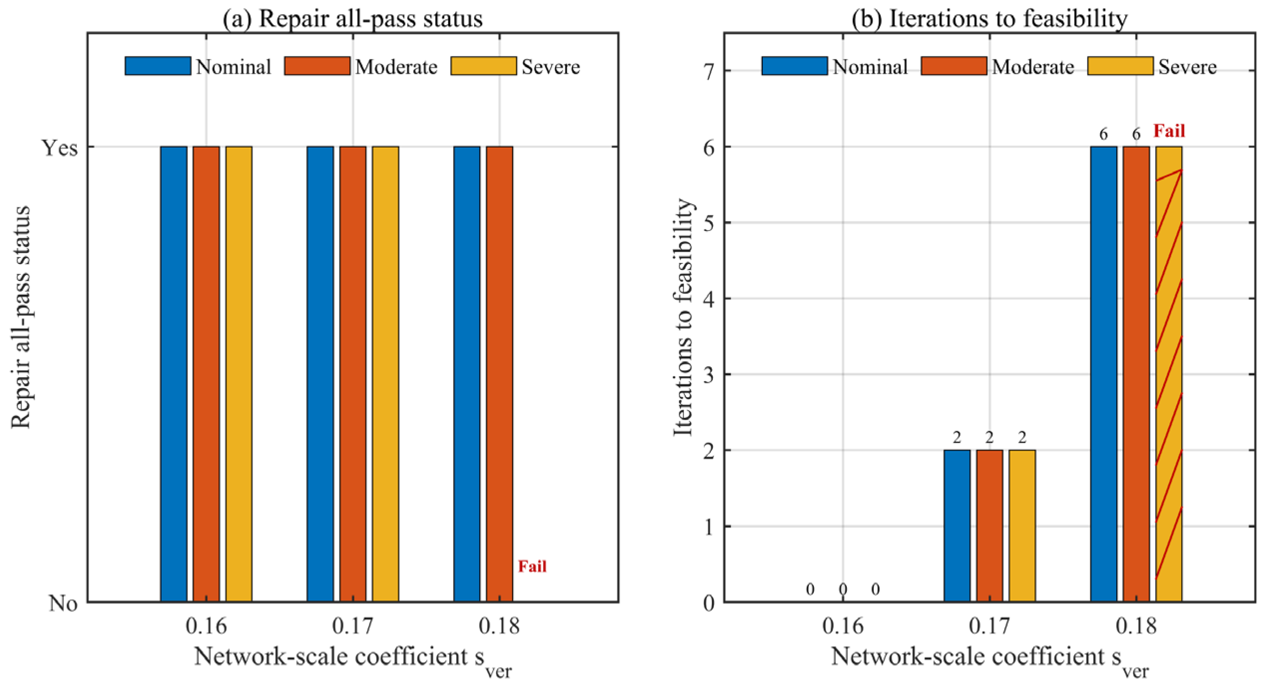
Under the calibrated posterior-verification setting with S v e r = 0.18, the three test scenarios all trigger power-network violations in the initial verification, whereas the gas and heating networks remain non-binding. The initial critical-hour minimum voltage is 0.946210 p.u. for all three scenarios, and the corresponding initial cumulative voltage violation is 0.003790. After the closed-loop repair with the baseline shrinking factor η r e p = 0.90, the nominal and moderate scenarios are restored to full feasibility within six iterations, while the severe scenario still retains a residual voltage violation. These results indicate that the distribution network is the dominant vulnerable layer in the present case, whereas the gas and heating networks mainly provide auxiliary physical screening. The calibrated posterior-verification and repair outcomes under S v e r = 0.18 are summarized in Table 4.

5.5.2. Analysis of Distribution-Network Verification Results

The distribution network is the dominant bottleneck under the calibrated baseline setting. As shown in Figure 11, the lower-voltage boundary is the main source of infeasibility, whereas the upper-voltage boundary remains non-binding. This indicates that the physical risk introduced by the compromise scheduling solution is mainly reflected in the tightening of the low-voltage margin of the benchmark feeder.
Under S v e r = 0.18 and η r e p = 0.90, the nominal scenario is repaired from an initial minimum voltage of 0.946210 p.u. to a final minimum voltage of 0.951428 p.u., with the cumulative voltage violation reduced from 0.003790 to zero. The moderate scenario is also restored to full feasibility, with the final minimum voltage reaching 0.950401 p.u. By contrast, the severe scenario remains infeasible after six repair iterations, with a final minimum voltage of 0.947306 p.u. and a residual cumulative voltage violation of 0.002694.
These results indicate that the proposed repair strategy is effective for mild-to-moderate voltage violations under the calibrated baseline setting, while a clear recovery boundary still exists under more stressed conditions. Therefore, the severe scenario is interpreted as a stress-testing case rather than as the baseline operating condition.

5.5.3. Analysis of Gas- and Heating-Network Verification Results

Compared with the distribution network, the gas and heating networks do not trigger posterior infeasibility in the present case. For the gas network, the pressure margins remain positive under all tested scenarios, although the minimum upper-pressure margin is relatively small, reaching 2.539398 kPa. This indicates that the gas network is feasible but operates relatively closer to its upper-pressure boundary.
The heating network also remains non-binding. The minimum supply-side temperature margin is 14.230307 °C, and the minimum return-side temperature margin is 9.997410 °C for all three scenarios. Both margins remain positive with negligible scenario-to-scenario variation, indicating that the thermal side retains sufficient physical redundancy throughout the day.
Taken together, the posterior-verification results show a clear hierarchy among the three physical layers: the distribution network is the dominant bottleneck, whereas the gas and heating networks mainly provide complementary physical screening. Therefore, the closed-loop repair process is primarily triggered by power-network voltage violations. The detailed margin profiles of the gas and heating networks are provided in the Supplementary Materials.

5.6. Sensitivity Analysis of Calibration and Repair Parameters

To examine the influence of posterior-verification calibration and repair-parameter selection, this section compares different values of the network-scale coefficient S v e r and the shrinking factor η r e p . The main-text baseline setting is S v e r = 0.18 and η r e p = 0.90, while S v e r = 0.16 and 0.17, as well as η r e p = 0.85 and 0.95, are used only for sensitivity analysis.

5.6.1. Network-Scale Sensitivity

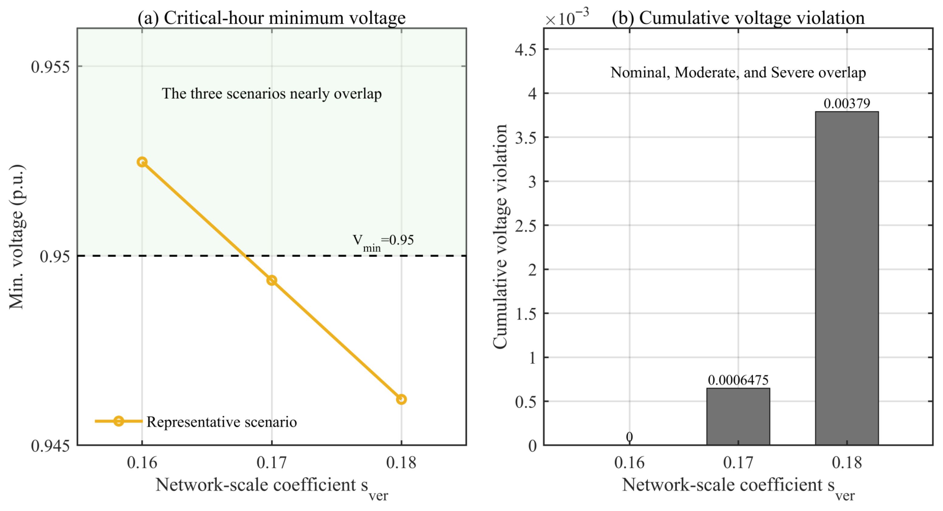
As shown in Figure 12, increasing S v e r strengthens the mapped loading level of the benchmark distribution network. The critical-hour minimum voltage decreases from 0.952475 p.u. at S v e r = 0.16 to 0.949352 p.u. at S v e r = 0.17, and further to 0.946210 p.u. at S v e r = 0.18. Meanwhile, the initial cumulative voltage violation increases from 0 to 0.000648 and then to 0.003790.
At S v e r = 0.16, all scenarios pass posterior verification directly, indicating a relatively mild verification condition. At S v e r = 0.17, the voltage violation is detectable but can be repaired within two iterations. At S v e r = 0.18, the nominal and moderate scenarios remain repairable, whereas the severe scenario cannot be fully recovered within the default repair budget. Therefore, S v e r = 0.18 is retained as the baseline setting because it reveals the voltage bottleneck while preserving repairability under mild-to-moderate stress. The red line denotes the lower-voltage safety boundary used for posterior verification.

5.6.2. Shrinking-Factor Sensitivity Under the Default Repair Limit

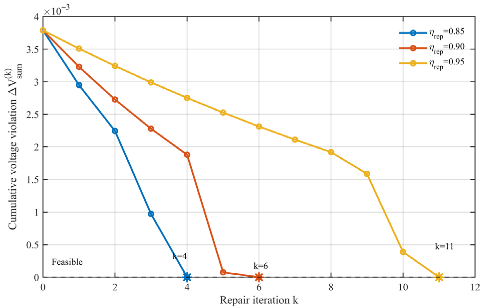
With S v e r fixed at 0.18, the influence of η r e p is compared in Table 5. A smaller η r e p gives a stronger boundary contraction and faster repair, while a larger η r e p results in a milder but slower update. Specifically, η r e p = 0.85 restores the nominal and moderate scenarios within four iterations, whereas η r e p = 0.95 cannot eliminate the voltage violation within the default six iterations. The baseline value η r e p = 0.90 provides an intermediate behavior and restores the nominal and moderate scenarios within K r e p max = 6.
The severe scenario remains infeasible within six iterations for all tested shrinking factors, indicating that the repair outcome also depends on the severity of the mapped network stress. Under more stressed conditions, additional operational flexibility, a larger repair-iteration limit, or a modified repair policy may be required.
It should be emphasized that the severe scenario is not used as the baseline operating condition, but as a stress-testing case for identifying the applicability boundary of the default repair setting. Under this condition, simply adjusting η r e p within the tested range cannot fully restore feasibility within K r e p max = 6. For more stressed operating conditions, alternative repair strategies may be required, such as increasing the repair-iteration budget, applying stronger multi-boundary contraction, coordinating storage dispatch and renewable curtailment, introducing demand-side flexibility, or embedding selected voltage-support constraints into the scheduling model. These strategies are beyond the default repair setting adopted in this study and will be further investigated in future work.

5.6.3. Extended Convergence Behavior

To illustrate the convergence trend, the moderate scenario under S v e r = 0.18 is extended beyond the default repair limit for visualization only. As shown in Figure 13, the cumulative voltage violation decreases monotonically for all three shrinking factors. The first feasible iteration occurs at k = 4 for η r e p = 0.85, at k = 6 for η r e p = 0.90, and at k = 11 for η r e p = 0.95. The corresponding minimum voltages at the feasible iteration are 0.950401, 0.950401, and 0.950746 p.u., respectively.
These results show that the closed-loop repair process exhibits a clear empirical convergence trend under the calibrated moderate scenario, while the shrinking factor mainly affects the repair speed. This extended test is used only to visualize the convergence tendency; the formal maximum repair iteration number in the manuscript remains K r e p max = 6.
Although the case study is based on a typical operating day of one industrial park, the proposed scheduling–verification–repair framework is modular and can be extended to other RIES configurations by updating device parameters, load profiles, price or emission settings, and physical network models. The sensitivity analyses under different network-scale coefficients, shrinking factors, and stress scenarios further show that the method can reflect changes in operating conditions and identify the applicability boundary of the default repair setting. Nevertheless, the quantitative results remain case-dependent, and further validation under multi-season, multi-day, and uncertain operating conditions will be considered in future work.

6. Conclusions

This paper proposes an integrated scheduling–verification–repair framework for regional integrated energy systems. A bi-objective MILP model is first established to characterize the trade-off between operating cost and carbon emissions, and an adaptive ε-constraint strategy is adopted to improve the local resolution of the compromise region. The case results show that the refined scanning strategy improves the resolution of the compromise region by 3.2 times with only a 20.4% increase in computational time, thereby improving the reliability of compromise-solution identification.
The posterior verification results show that scheduling-layer feasibility based on energy-balance constraints does not necessarily guarantee physical-network feasibility. Under the calibrated baseline setting, the dominant infeasibility is associated with the lower-voltage boundary of the distribution network, while the gas and heating networks remain feasible and mainly provide complementary physical screening. The closed-loop repair mechanism further improves the physical implementability of the representative scheduling solution. Under S v e r = 0.18 and η r e p = 0.90, the nominal and moderate scenarios are restored to feasibility within six iterations, whereas the severe scenario still retains a residual voltage violation after the default repair budget is exhausted. This indicates the applicability boundary of the current repair setting under more stressed operating conditions.
Sensitivity analysis shows that S v e r affects the triggering intensity of posterior verification, while η r e p influences the repair speed and boundary-contraction intensity. The extended convergence results further show a monotonic reduction in cumulative voltage violation under the calibrated moderate scenario, supporting the empirical stability of the proposed repair procedure. Although the present validation is based on a typical-day case study, the modular scheduling–verification–repair framework can be extended to other RIES configurations by updating device parameters, operating scenarios, and network models. Future work will further validate the method under multi-season, multi-day, and uncertain operating conditions, and develop advanced repair strategies, such as multi-boundary repair, demand-side flexibility, and selected network-constrained re-optimization, to better balance feasibility restoration and scheduling optimality.


Supplementary Materials

The following supporting information can be downloaded at https://www.mdpi.com/article/10.3390/en19102381/s1. The supplementary package includes Supplementary Material, which contains detailed network data, interface-mapping information, supplementary verification results, and additional tables and figures; and Supplementary_Data, which contains the README file, input data, output tables, and original output figures used in this study.

Author Contributions

Conceptualization, M.Z.; methodology, Q.W.; software, Q.W.; validation, Q.W., H.W. and Y.Z.; formal analysis, Q.W.; investigation, Q.W., H.W. and Y.Z.; resources, M.Z.; data curation, H.W. and Y.Z.; writing—original draft preparation, Q.W.; writing—review and editing, M.Z., Q.W., H.W. and Y.Z.; visualization, Q.W.; supervision, M.Z.; project administration, M.Z.; funding acquisition, M.Z. All authors have read and agreed to the published version of the manuscript.

Funding

This research was funded by the National Natural Science Foundation of China, grant number 72464020.

Data Availability Statement

The data supporting the findings of this study are available in the Supplementary Materials. Additional materials are available from the corresponding author upon reasonable request. The source code is not publicly available in this submission.

Conflicts of Interest

Author Hao Wang was employed by Huanxian Power Supply Company, State Grid Gansu Electric Power Company. Author Yinyin Zhao was employed by Xifeng District Power Supply Company, State Grid Gansu Electric Power Company. The authors declare that this employment relationship did not influence the study design, data analysis, interpretation of results, or conclusions of the manuscript. The remaining authors declare that the research was conducted in the absence of any commercial or financial relationships that could be construed as a potential conflict of interest.

Nomenclature

Indices
SymbolMeaningUnit
t scheduling time index
i , j indices of distribution network nodes
m , n indices of gas network nodes
Main scheduling variables
P b u y , t purchased electricity power MW
P s e l l , t sold electricity power MW
P p e a k maximum purchased electricity power during the scheduling horizon MW
V g a s , t natural gas consumption volume m 3
G t o t a l , t total natural gas energy consumption of the system MWh
P g t , t power output of the gas turbine MW
G G T , t natural gas energy consumption of the gas turbine MWh
H h r b , t recovered thermal power of the heat recovery boiler MW
H g b , t heat output of the gas boiler MW
G G B , t natural gas energy consumption of the gas boiler MWh
L a c , t cooling output of the absorption chiller MW
L e c , t cooling output of the electric chiller MW
P p v , t actual photovoltaic output MW
P ω t , t actual wind power output MW
P c h , t , P d i s , t charging/discharging power of the energy storage system MW
S O C t state of charge of the energy storage system
Economic and emission parameters
C e , t electricity purchase price at time period t CNY / kWh
C g , t natural gas purchase price at time period t CNY / m 3
C s e l l , t electricity selling price at time period t CNY / kWh
C p e a k demand charge CNY / ( kW day )
λ c u r t penalty coefficient for renewable curtailment CNY / kWh
μ e carbon emission factor of grid electricity tC O 2 / MWh
μ g carbon emission factor of natural gas tC O 2 / MWh
e E C I , t effective carbon emission intensity of gas turbine power generation at time period t tC O 2 / MWh
η r e p outer-layer boundary shrinking factor
K r e p max maximum number of repair iterations
S v e r network-scale coefficient for posterior power-network verification
Load and renewable variables
P l o a d , t electric load MW
H l o a d , t thermal load MW
L l o a d , t cooling load MW
P p v , a v a , t available photovoltaic output MW
P ω t , a v a , t available wind power output MW
Main device parameters
η e , g t power generation efficiency of the gas turbine
η h r b heat recovery coefficient of the heat recovery boiler
η g b thermal efficiency of the gas boiler
C O P a c coefficient of performance of the absorption chiller
C O P e c coefficient of performance of the electric chiller
R a m p G T ramp-rate limit of the gas turbine MW / h
S O C ¯ , S O C ¯ lower and upper bounds of energy storage state of charge
Physical validation variables
V i voltage magnitude at distribution network node i   p . u . p . u .
P i j , Q i j active and reactive power flows of branch i j   MW , Mvar MW , Mvar
f m , f n gas pressure at gas network nodes kPa kPa
F m n gas flow rate in pipeline m n   kg / s kg / s
m ˙ i j mass flow rate in heating pipeline ij kg / s kg / s
T s , i , T r , i supply and return water temperatures at heating network node i °C°C

Abbreviations

SymbolMeaning
RIESregional integrated energy system
GTgas turbine
HRBheat recovery boiler
GBgas boiler
ACabsorption chiller
ECelectric chiller
ESSenergy storage system
ECIeffective carbon emission intensity

Appendix A. Summary of System Device, Price, and Evaluation Parameters

Table A1. Summary of major system devices, prices, and evaluation parameters.
CategoryParameter (Symbol)ValueUnitDescription
Gas turbine (GT)Rated power output ( P g t max )18 M W Main local power-generation unit
Electrical efficiency ( η e , g t )0.26GT power-generation efficiency
Heat-recovery coefficient ( η h r b )0.68Fraction of recoverable waste heat
Ramp-rate limit ( R a m p G T )6MW/hMaximum hourly ramping capability
Heat recovery boiler (HRB)Maximum recovered heat output ( H h r b max )43 MW Upper limit of recovered thermal power
Gas boiler (GB)Minimum heat output ( H g b min )9 MW Lower operating limit
Maximum heat output ( H g b max )36 MW Upper operating limit
Thermal efficiency ( η g b )0.85Gas-to-heat conversion efficiency
Absorption chiller (AC)Maximum cooling output ( L a c max )20 MW Heat-driven cooling
Absorption chiller COP ( C O P a c )0.80Performance coefficient of AC
Electric chiller (EC)Maximum electric input ( P e c , i n max )30 MW Electric-driven cooling
Electric chiller COP ( C O P e c )3.0Performance coefficient of EC
Energy storage system (ESS)Energy capacity ( E b a t )6 MWh Installed storage capacity
Charging/discharging power limit1.5 MW Power upper bound
Charging efficiency ( η c h )0.90Charging efficiency
Discharging efficiency ( η d i s )0.85Discharging efficiency
Initial state of charge ( S O C 0 )0.30Initial SOC
SOC lower/upper bounds ( S O C ¯ , S O C ¯ )[0.10,0.90]Safe operating interval
Electricity priceOff-peak/Flat-period/Peak-period purchase price ( C e , t )0.333/0.6368/1.0041 CNY / kWh TOU tariff
Selling price ( C s e l l , t )0.4146 CNY / kWh Feed-in tariff
Demand charge ( C p e a k )0.2 CNY / ( kW day ) Daily maximum-demand charge
Peak-period purchase upper bound ( P g r i d , p e a k max )10 MW Peak-period purchase limit
Grid-interaction upper bound ( P g r i d , max )15 MW Grid-interaction capacity limit
Natural gasGas purchase price ( C g , t )2.5 CNY / m 3 Fixed gas price
Lower heating value ( L H V )0.0097 MWh / m 3 Energy–volume conversion coefficient
Carbon-emission factorsGrid electricity carbon factor ( μ e )0.7035 tC O 2 / MWh Grid-side carbon intensity
Natural-gas carbon factor ( μ g )0.4483 tC O 2 / MWh Gas-side carbon intensity
Repair settingCurtailment penalty coefficient ( λ c u r t )1.2 CNY / kWh Penalty on wind/PV curtailment
Gas-purchase upper bound ( G b u y , max )(106) m 3 / h Large upper bound used in repair
These parameters are used consistently in the scheduling model and provide the operating inputs for posterior verification. The calibration and repair settings used in posterior verification and Auto-Repair are summarized separately in Appendix B.

Appendix B. Key Settings for Posterior Verification and Feedback Repair

For brevity, only the key settings required for interpreting the posterior verification and feedback repair results are summarized in this appendix. Detailed network data, nodal and branch parameters, interface-mapping details, and full implementation settings are provided in the Supplementary Material.
Table A2. Main posterior-verification and feedback-repair settings.
ItemSetting/ValueRemark
Distribution benchmark modelIEEE 33-bus systemUsed for posterior power-flow verification
Gas benchmark model14-node gas networkUsed for gas-pressure verification
Heating benchmark model17-node heating networkUsed for thermo-hydraulic verification
Coupling interfacesAs listed in Table 1EH-based interface mapping between scheduling and physical networks
Margin indicesVoltage margin, pressure margin, and temperature marginDefined by Equations (35)–(37)
Coarse ε-scan samples20Used for global Pareto-front screening
Refined ε-scan samples25Used for local refinement in the compromise region
Main network-scale coefficient0.18Baseline setting used for main-text posterior power network verification
Calibration sensitivity coefficients0.16, 0.17Used only for calibration sensitivity analysis
Baseline shrinking factor0.90Baseline boundary-shrinking factor used in Auto-Repair
Shrinking-factor comparison0.85, 0.95Used only for repair parameter sensitivity analysis
Maximum repair iterations6Upper bound of the Auto-Repair process
Main repair targetsElectricity-purchasing and gas-purchasing boundariesIn the studied case, the heating network does not constitute the dominant bottleneck
Heating-network repair statusNot activated in the reported caseHeating-network temperature margins remain positive; heat-boundary repair can be extended for other operating conditions

References

  1. Shao, C.C.; Wang, X.F.; Wang, X.L.; Wang, B.Y. A first look at multi-energy system analysis and planning. Proc. CSEE 2016, 36, 3817–3829. [Google Scholar] [CrossRef]
  2. Liu, D.C.; Peng, S.C.; Liao, Q.F.; Tang, F.; Chen, W.; Chen, Y. Outlook for the future shape of integrated power distribution system for energy internet. Power Syst. Technol. 2015, 39, 3023–3034. [Google Scholar] [CrossRef]
  3. Liu, Z.-F.; Liu, Y.-Y.; Jia, H.-J.; Jin, X.-L.; Liu, T.-H.; Wu, Y.-Z. Bi-level energy co-optimization of regional integrated energy system with electric vehicle to generalized-energy conversion framework and flexible hydrogen-blended gas strategy. Appl. Energy 2025, 390, 125868. [Google Scholar] [CrossRef]
  4. Li, Z.; Xu, Y.; Wang, P.; Xiao, G. Coordinated preparation and recovery of a post-disaster multi-energy distribution system considering thermal inertia and diverse uncertainties. Appl. Energy 2023, 336, 120736. [Google Scholar] [CrossRef]
  5. Li, B.; Li, X.; Su, Q. A system and game strategy for the isolated island electric-gas deeply coupled energy network. Appl. Energy 2022, 306, 118013. [Google Scholar] [CrossRef]
  6. Kang, L.; Wang, J.; Yuan, X.; Cao, Z.; Yang, Y.; Deng, S.; Zhao, J.; Wang, Y. Research on energy management of integrated energy system coupled with organic Rankine cycle and power to gas. Energy Convers. Manag. 2023, 287, 117117. [Google Scholar] [CrossRef]
  7. Zhang, B.; Li, J.; Zhang, L.; Tang, W.; Sun, Y. Reliability evaluation of electric-gas-thermal coupling systems considering the post-fault operation modes of user-level integrated energy system. iScience 2024, 27, 110922. [Google Scholar] [CrossRef]
  8. Yilmaz, C.; Arslan, M.; Ozdemir, S.N.; Tokgoz, N. Thermal design and genetic algorithm optimization of geothermal and solar-assisted multi-energy and hydrogen production using artificial neural networks. Energy 2025, 324, 135941. [Google Scholar] [CrossRef]
  9. Chen, J.; Li, K.; Wang, H.; Zhao, D.; Jiang, C.; Zhang, C. Distributed parallel optimal operation for shared energy storage system-multiple park integrated energy system based on ADMM. Energy 2025, 317, 134677. [Google Scholar] [CrossRef]
  10. Yang, D.; Wang, X.; Sun, Y.; Yang, J.; Liu, X.; Jiang, C. Optimised configuration of multi-energy systems considering the adjusting capacity of communication base stations and risk of network congestion. Energy 2024, 313, 133873. [Google Scholar] [CrossRef]
  11. Xu, X.; Xu, K.; Zeng, Z.; Tang, J.; He, Y.; Shi, G.; Zhang, T. Collaborative optimization of multi-energy multi-microgrid system: A hierarchical trust-region multi-agent reinforcement learning approach. Appl. Energy 2024, 375, 123923. [Google Scholar] [CrossRef]
  12. Liu, J.; Tang, Z.; Liu, Y.; Zhou, Y.; Zeng, P.P.; Wu, Q. Region-inspired distributed optimal dispatch of flexibility providers in coordinated transmission-distribution framework. Energy 2025, 319, 134985. [Google Scholar] [CrossRef]
  13. Yue, W.; Yu, S.; Xu, M.; Rong, Q.; Xu, C.; Su, M. A Copula-based interval linear programming model for water resources allocation under uncertainty. J. Environ. Manag. 2022, 317, 115318. [Google Scholar] [CrossRef]
  14. Esfahani, M.; Alizadeh, A.; Amjady, N.; Kamwa, I. A distributed VPP-integrated co-optimization framework for energy scheduling, frequency regulation, and voltage support using data-driven distributionally robust optimization with Wasserstein metric. Appl. Energy 2024, 361, 122883. [Google Scholar] [CrossRef]
  15. Ahmadi, A.; Charwand, M.; Siano, P.; Nezhad, A.E.; Sarno, D.; Gitizadeh, M.; Raeisi, F. A novel two-stage stochastic programming model for uncertainty characterization in short-term optimal strategy for a distribution company. Energy 2016, 117, 1–9. [Google Scholar] [CrossRef]
  16. Siface, D.; Vespucci, M.T.; Gelmini, A. Solution of the mixed integer large scale unit commitment problem by means of a continuous stochastic linear programming model. Energy Syst. 2014, 5, 269–284. [Google Scholar] [CrossRef]
  17. Xiang, L. A large-scale equilibrium model of energy emergency production: Embedding social choice rules into Nash Q-learning automatically achieving consensus of urgent recovery behaviors. Energy 2022, 259, 125023. [Google Scholar] [CrossRef]
  18. Zheng, J.; Zhou, Z.; Zhao, J.; Wang, J. Effects of the operation regulation modes of district heating system on an integrated heat and power dispatch system for wind power integration. Appl. Energy 2018, 230, 1126–1139. [Google Scholar] [CrossRef]
  19. Deng, Z.; Wang, X.; Dong, B. Integrating quantum computing into building-to-grid control framework: Application of benders decomposition in mixed-integer nonlinear programming. Build. Simul. 2025, 18, 1163–1178. [Google Scholar] [CrossRef]
  20. Teymoori, H.F.; Safari, A.; Kamalinasab, M. Augmented ε-constraint algorithm applied to multi-objective optimization programs of residential micro-CHP systems. Process Integr. Optim. Sustain. 2022, 6, 1143–1161. [Google Scholar] [CrossRef]
  21. Ajith, J.; Nanda, S.J.; Maddila, R.K. A multi-objective natural aggregation algorithm for optimizing user allocation matrix in visible light communication. Optik 2022, 267, 169692. [Google Scholar] [CrossRef]
  22. Ren, X.; Wang, M.; Dai, G.; Peng, L.; Chen, X.; Song, Z. Multi-objective evolutionary algorithm based on transfer learning and neural networks: Dual operator feature fusion and weight vector adaptation. Inf. Sci. 2025, 686, 121364. [Google Scholar] [CrossRef]
  23. Oh, B.C.; Son, Y.G.; Acquah, M.A.; Kim, S.Y. A new framework for hierarchical multi-objective energy hub planning considering reliability. Energy 2024, 303, 131889. [Google Scholar] [CrossRef]
  24. Xu, G.; Yang, Z. Risk-aware low carbon optimization of hydrogen-oriented multi-energy system with linear approximation of bi-product fuel cell. Energy 2025, 334, 137581. [Google Scholar] [CrossRef]
  25. Mavrotas, G.; Florios, K. An improved version of the augmented ε-constraint method (AUGMECON2) for finding the exact pareto set in multi-objective integer programming problems. Appl. Math. Comput. 2013, 219, 9652–9669. [Google Scholar] [CrossRef]
  26. Shahbazian, R.; Ciacco, A.; Macrina, G.; Guerriero, F. Knowledge-guided hybrid deep reinforcement learning for the dynamic multi-depot electric vehicle routing problem. Comput. Oper. Res. 2025, 184, 107217. [Google Scholar] [CrossRef]
  27. Lv, Z.; Liao, Z.; Liu, Y.; Zhao, J. Meta-learning-based multi-objective PSO model for dynamic scheduling optimization. Energy Rep. 2023, 9, 1227–1236. [Google Scholar] [CrossRef]
  28. Liu, C.; Wang, Y.; Xie, K. Multi-Objective Reinforcement Learning for Optimal Scheduling of Electricity-Hydrogen-Thermal Multi-Energy Microgrids. In Proceedings of the 2024 IEEE/IAS Industrial and Commercial Power System Asia (I&CPS Asia), Pattaya, Thailand, 9–12 July 2024. [Google Scholar] [CrossRef]
  29. Deng, B.; Xu, X.; Li, M.; Ji, T.; Wu, Q.H. Two-stage multi-objective optimization and decision-making method for integrated energy system under wind generation disturbances. CSEE J. Power Energy Syst. 2024, 10, 2564–2576. [Google Scholar] [CrossRef]
  30. Ciacco, A.; Guerriero, F.; Osaba, E. Steiner Traveling Salesman Problem with Quantum Annealing. In Proceedings of the Genetic and Evolutionary Computation Conference Companion (GECCO ’25 Companion), Malaga, Spain, 14–18 July 2025; Association for Computing Machinery: New York, NY, USA, 2025; pp. 2412–2418. [Google Scholar] [CrossRef]
  31. Lucas, A. Ising formulations of many NP problems. Front. Phys. 2014, 2, 5. [Google Scholar] [CrossRef]
  32. Xu, X.; Hou, K.; Jia, H.; Yu, X. A reliability assessment approach for the urban energy system and its application in energy hub planning. In Proceedings of the 2015 IEEE Power & Energy Society General Meeting, Denver, CO, USA, 26–30 July 2015; pp. 1–5. [Google Scholar] [CrossRef]
  33. Wang, S.; Ding, Y.; Ye, C.; Wan, C.; Mo, Y. Reliability evaluation of integrated electricity-gas system utilizing network equivalent and integrated optimal power flow techniques. J. Mod. Power Syst. Clean Energy 2019, 7, 1523–1535. [Google Scholar] [CrossRef]
  34. Yan, C.; Bie, Z.; Liu, S.; Urgun, D.; Singh, C.; Xie, L. A reliability model for integrated energy system considering multi-energy correlation. J. Mod. Power Syst. Clean Energy 2021, 9, 811–825. [Google Scholar] [CrossRef]
  35. Paterakis, N.G.; Mazza, A.; Santos, S.F.; Erdinç, O.; Chicco, G.; Bakirtzis, A.G.; Catalão, J.P.S. Multi-Objective Reconfiguration of Radial Distribution Systems Using Reliability Indices. IEEE Trans. Power Syst. 2016, 31, 1048–1062. [Google Scholar] [CrossRef]
  36. Wang, C.; Huang, Y.; Zhang, B.; Rong, X.; E, L.; Ning, D.; Li, G. Carbon Emission Accounting for Integrated Energy Systems Considering Network Interconnection. In Proceedings of the 2024 IEEE 8th Conference on Energy Internet and Energy System Integration (EI2), Shenyang, China, 29 November–2 December 2024; pp. 567–572. [Google Scholar] [CrossRef]
  37. Long, T.; Bie, Z.; Jiang, L.; Wang, X.; Li, G. Multi-scenario planning of integrated energy distribution network based on DistFlow model. In Proceedings of the 2022 4th Asia Energy and Electrical Engineering Symposium (AEEES), Chengdu, China, 25–28 March 2022; pp. 773–779. [Google Scholar] [CrossRef]
  38. Liu, G.; Li, Z. Chance-constrained optimal power flow for an integrated transmission and distribution network. In Proceedings of the 2023 International Conference on Power Energy Systems and Applications (ICoPESA), Nanjing, China, 24–26 February 2023; pp. 382–387. [Google Scholar] [CrossRef]
  39. Blanco-Martínez, C.A.; Álvarez-Meza, A.M.; Castellanos-Dominguez, G.; Cárdenas-Peña, D.A.; Orozco-Gutiérrez, Á.A. Optimization of interconnected natural gas and power systems using mathematical programs with complementarity constraints. Mathematics 2024, 12, 2224. [Google Scholar] [CrossRef]
  40. Zhang, S.; Chen, S.; Gu, W.; Lu, S.; Chung, C.Y. Dynamic optimal energy flow of integrated electricity and gas systems in continuous space. Appl. Energy 2024, 375, 124052. [Google Scholar] [CrossRef]
  41. Pałka, P.; Malec, M.; Kaszyński, P.; Kamiński, J.; Saługa, P. District heating system optimisation: A three-phase thermo-hydraulic linear model. Energies 2023, 16, 3316. [Google Scholar] [CrossRef]
  42. Wang, Z.; Zhang, N.; Zhang, Y.; Lin, X.; Qin, F. A study on hydraulic balance optimization of district heating system based on data-mechanism fused model. In Proceedings of the 2021 IEEE 5th Conference on Energy Internet and Energy System Integration (EI2), Taiyuan, China, 22–24 October 2021; pp. 4046–4050. [Google Scholar] [CrossRef]
Figure 1. Architecture of the regional integrated energy system (RIES).
Energies 19 02381 g001
Figure 2. Closed-loop scheduling framework with posterior physical verification and feedback repair for RIES.
Energies 19 02381 g002
Figure 3. Hierarchical Coupling Network Topology of RIES.
Energies 19 02381 g003
Figure 4. Typical daily load profile.
Energies 19 02381 g004
Figure 5. Electricity and natural gas price curves.
Energies 19 02381 g005
Figure 6. Cost–carbon Pareto front. The dotted box highlights the locally refined compromise region enlarged in Figure 7.
Energies 19 02381 g006
Figure 7. Locally refined compromise region of the cost–carbon Pareto front.
Energies 19 02381 g007
Figure 8. Relationship between peak purchased electricity power and carbon-emission constraint.
Energies 19 02381 g008
Figure 9. Normalized comparison between baseline and optimized strategies.
Energies 19 02381 g009
Figure 10. Total 24 h multi-energy balance under the compromise solution.
Energies 19 02381 g010
Figure 11. Power-network posterior verification under calibrated scales.
Energies 19 02381 g011
Figure 12. Network-scale sensitivity of posterior verification and repair outcomes.
Energies 19 02381 g012
Figure 13. Extended convergence behavior of the closed-loop repair process under different shrinking factors.
Energies 19 02381 g013
Table 1. Configuration of system networks and coupling interfaces.
Energy LayerDistribution NetworkGas NetworkHeating Network
Benchmark modelIEEE 33-bus system14-node gas network17-node heating network
Core node configurationEH1 connected to Node 25EH1 connected to Node 3;
EH2 connected to Node 13
EH2 connected to Node 15
Table 2. Summary of representative solutions (Cost/Carbon/Peak Grid).
SolutionCost (CNY)Carbon (t)Peak Grid (MW)Index_J
Baseline-Price281,453.78490.2610.30.9511
Baseline-Smooth286,149.55497.730.001.3095
Opt-Cost281,211.492491.3207.3331.0000
Opt-Carbon307,944.084469.69811.11.0000
Opt-Compromise289,208.46477.6649.2160.4746
Table 3. Performance comparison of different scanning strategies.
Scanning StrategyNumber of SamplesCandidate/Effective SolutionsResolution in Compromise RegionComputational Time Increase
Conventional ε-constraint method (coarse scan)2020Baseline (1.0×)
Adaptive ε-constraint method (coarse + refined scan)45443.2×+20.4%
Table 4. Calibrated posterior-verification and repair outcomes under S v e r = 0.18.
ScenarioInitial All-PassDominant Violated NetworkInitial Minimum Voltage (p.u.)Initial Cumulative Voltage ViolationViolation Duration (h)Repair All-Pass ( η r e p   =   0.90 )Repair IterationsFinal Minimum Voltage (p.u.)Final Cumulative Voltage Violation
NominalFAILPower0.9462100.0037901PASS60.9514280.000000
ModerateFAILPower0.9462100.0037901PASS60.9504010.000000
SevereFAILPower0.9462100.0037901FAIL60.9473060.002694
Table 5. Shrinking-factor sensitivity under the default repair limit ( S v e r = 0.18 ).
η r e p ScenarioInitial Cumulative Voltage ViolationFinal Cumulative Voltage ViolationRepair IterationsFinal All-Pass
0.95Nominal0.0037900.0023136FAIL
0.90Nominal0.0037900.0000006PASS
0.85Nominal0.0037900.0000004PASS
0.95Moderate0.0037900.0023136FAIL
0.90Moderate0.0037900.0000006PASS
0.85Moderate0.0037900.0000004PASS
0.95Severe0.0037900.0023136FAIL
0.90Severe0.0037900.0026946FAIL
0.85Severe0.0037900.0026946FAIL
Disclaimer/Publisher’s Note: The statements, opinions and data contained in all publications are solely those of the individual author(s) and contributor(s) and not of MDPI and/or the editor(s). MDPI and/or the editor(s) disclaim responsibility for any injury to people or property resulting from any ideas, methods, instructions or products referred to in the content.