Article

Development and Validation of a Physical Model Optimized by Evolutionary Algorithms for the Accurate Estimation of Cell Temperature in Photovoltaic Systems


by
Doroteya Dimitrova-Angelova
1,
Diego Carmona Fernández
1,
Manuel Calderón Godoy
1,
Juan Antonio Álvarez Moreno
1 and
Juan Félix González González
2,*
1
Department of Electrical Engineering, Electronics and Automation, Industrial Engineering School, University of Extremadura, Avenida de Elvas s/n, 06006 Badajoz, Spain
2
Department of Applied Physics, Industrial Engineering School, University of Extremadura, Avenida de Elvas s/n, 06006 Badajoz, Spain
*
Author to whom correspondence should be addressed.
Energies 2026, 19(10), 2286; https://doi.org/10.3390/en19102286
Submission received: 17 April 2026 / Revised: 1 May 2026 / Accepted: 6 May 2026 / Published: 9 May 2026
(This article belongs to the Topic Sustainable Energy Systems)

Abstract

Accurate photovoltaic cell temperature estimation is critical for maximizing energy management and improving digital twin fidelity in building-integrated solar systems. Classical models, NOCT (Nominal Operating Cell Temperature), King, Skoplaki, and PVsyst/Faiman, provide a practical baseline but exhibit significant limitations when applied to complex, real-world scenarios. These static and linear approaches fail to capture dynamic thermal phenomena such as thermal inertia, nonlinear irradiance effects, and wind-temperature interactions. This paper presents an advanced physical model that incorporates thermal memory effects, sophisticated wind modeling, transient cloud-response mechanisms, and non-linear thermal dependencies. Parameter calibration was performed using a differential evolution algorithm, automatically optimizing the model fit to one year of experimental data from a 2.79 kW pilot installation at the University of Extremadura. The validation results demonstrate consistent improvements across all seasons: RMSE reductions of up to 4.9% and MAE reductions of up to 14.4% compared to classical approaches, with particularly pronounced gains during the summer and autumn. The methodology is readily transferable to diverse installations and climatic contexts, providing a robust framework for developing high-accuracy PV digital twins and enabling early fault detection and operational optimization.

1. Introduction

Reducing CO2 emissions in buildings is a priority for achieving the European Union’s targets: 55% reduction by 2030 and climate neutrality by 2050 [1]. Buildings account for approximately 36% of greenhouse gas emissions and 40% of total EU energy consumption [2], driving the need for widespread adoption of sustainable technologies and advanced energy management systems [3]. In this context, photovoltaic systems in buildings emerge as a key strategy for decarbonization and energy self-sufficiency [4].
Solar photovoltaic systems are essential for sustainable buildings, as they reduce fossil fuel consumption and increase energy self-sufficiency [5]. Recent growth has been remarkable: global installed PV capacity exceeded 2.2 TWp in 2024, with almost 600 GWp added that year, doubling in less than three years [6].
However, this rapid expansion brings new operational challenges. To maximize installation performance and ensure reliable energy delivery, advanced digital twins have become fundamental tools, enabling continuous monitoring, predictive analysis, and dynamic optimization [7]. However, their effectiveness essentially depends on the accurate estimation of the PV cell temperature, as temperature increases significantly reduce conversion efficiency and power output [8].
Direct temperature measurement in building-integrated modules presents challenges: the cells are encapsulated, preventing access to the actual operating temperature [9], and temperature distribution is not uniform across all modules [10]. While thermocouples and fiber optic sensors provide accuracy [11], they are expensive and require custom designs; distributed sensor networks are limited to specific applications [9]. Consequently, indirect estimation from meteorological and electrical variables offers greater practicality [12].
Beyond temperature, the nonlinearity of irradiance and spectral composition critically affect the modeling accuracy for building-integrated modules [13]. At low irradiance, temperature coefficients change nonlinearly [14], and spectral effects can reach variations of approximately 15% in winter, depending on the module technology and location [15]. Researchers have also explored alternatives such as spectral pyrometers, which eliminate emissive uncertainty by measuring infrared radiation across multiple wavelengths [16].
The most widely used temperature estimation models (NOCT, King, Skoplaki, and PVsyst/Faiman) employ different variables and assumptions [17]. The NOCT model prioritizes simplicity, considering only irradiance and ambient temperature [18]. However, wind speed plays a crucial role in thermal regulation, reducing the photovoltaic module temperature by up to 12 °C under strong wind conditions (especially with southerly/upwind winds) and improving efficiency by 6.5% to 7.2% [19]. Models incorporating wind speed (King and Skoplaki) demonstrate superior accuracy, particularly in warm climates [20]. Skoplaki allows for the calibration of coefficients for specific conditions, while PVsyst/Faiman implements modified formulations with convection and heat transfer parameters, facilitating adaptation to different installations [21]. However, despite their formal equivalence and widespread use under standard conditions, these classical models present critical limitations in complex real-world scenarios [22].
Building-integrated PV systems, environments with limited ventilation, and dynamic climatic conditions highlight fundamental shortcomings in classical models [23]: they rely on constant coefficients and linear relationships, failing to capture cloud cover, rapid irradiance transients, thermal inertia, and nonlinear interactions [24]. This inflexibility can lead to temperature estimation errors exceeding 10% in peak power prediction, directly compromising operational efficiency and decision-making in applications requiring high-fidelity monitoring [25]. Overcoming these limitations requires more advanced approaches that incorporate improved physical descriptions and dynamic parameter adaptation [26].
To address this gap, this work employs evolutionary algorithms for automated model calibration and parameter optimization. Evolutionary algorithms are particularly well-suited for this application because they excel at complex [27] and nonlinear [28] optimization problems, explore the solution space globally to avoid local optima, handle multiple variables and constraints efficiently [29], and enable knowledge transfer between similar problems for faster convergence and a superior solution [30]. Recent studies confirm their effectiveness in calibrating photovoltaic models, consistently outperforming traditional and metaheuristic techniques in accuracy [31], robustness, and convergence speed, even under complex and nonlinear conditions [32].
The main objective of this work is to analyze and compare the effectiveness of several mathematical models for estimating the temperature of photovoltaic cells, in order to identify and validate the most appropriate approach for building a digital twin of a 2.79 kW pilot installation located at the School of Industrial Engineering of the University of Extremadura. This installation, representative of photovoltaic systems in buildings, falls within the average range of contracted power in the Spanish residential sector (2.45–4.6 kW) [33], which reinforces the applicability and practical relevance of the results.
As an innovative contribution, this work develops and calibrates an advanced model for estimating PV cell temperature using evolutionary algorithms for automated parameterization. This approach efficiently identifies optimal combinations of coefficients that maximize the agreement between model predictions and experimental data, overcoming the limitations of classical methods and achieving robust and accurate estimates under varying environmental conditions. The model has been calibrated using real experimental data from the pilot installation, covering a full year and all seasons, ensuring its validity and adaptability to real-world operating scenarios. Furthermore, this methodology facilitates model recalibration with data from other installations, enabling flexible and transferable application in diverse climatic contexts. The proposed approach thus improves the fidelity of the digital twin for the analyzed installation, while providing a versatile tool for researchers and professionals to optimize energy management in various photovoltaic environments.

2. Materials and Methods

2.1. Data and Experimental Scenario

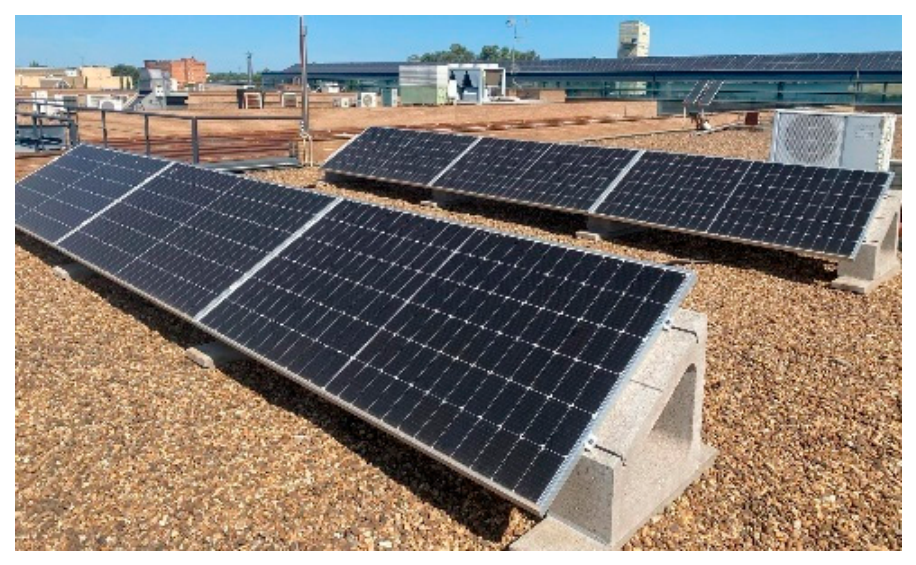
The methodology employed in this work consisted of the selection, sizing, and installation of a 2.79 kWp photovoltaic pilot system on the rooftop of the School of Industrial Engineering (latitude 38.884° N, longitude −7.004° E) at the University of Extremadura (see Figure 1). This south-facing installation, with a 30° tilt and 0° azimuth, comprises six monocrystalline panels JA Solar (Shanghai, China), connected in series and a three-phase inverter (Shenzhen, China), which supplies renewable energy to the Thermodynamics Laboratory and allows for grid injection. To monitor relevant environmental variables, a Vantage Pro2™ wireless weather station with Weatherlink Live [34] was used, capable of measuring irradiance, outdoor temperature, and wind speed. Additionally, a 3D-printed support was designed to hold the DAVIS 6450 pyranometer on the same tilted plane as the panels, thus ensuring accurate solar radiation measurements [35].
Table 1 shows the technical specifications of the measuring equipment. Meteorological data were recorded using a Davis Vantage Pro2 weather station. Regarding the direct current (DC) power obtained using the Huawei app, and considering the accuracy specified for Huawei ecosystem measuring equipment, on the order of ±1% for power and energy, the power displayed in the app should be interpreted as a monitoring value that may exhibit a similar or greater deviation, depending on the measurement point and operating conditions. Table 1 also summarizes the range, resolution, and nominal accuracy of the main sensors used: solar irradiance, ambient temperature, and wind speed.
Data acquisition was performed using two independent platforms, each recording data at 5 min intervals (Excel format): (1) meteorological data (temperature, irradiance, wind speed) from the Vantage Pro2 weather station via the WeatherLink Live platform, and (2) electrical power data from the Huawei FusionSolar inverter. Time synchronization between the two asynchronous sources was achieved by establishing a common UTC reference timestamp with linear interpolation for small time deviations (<30 s), allowing for direct comparison between measured and simulated power across 9316 observations over a full year.
Records with missing values for ambient temperature, irradiance, wind speed, and actual power were removed. Zero wind speed values were retained as valid measurements, and photovoltaic panel-specific parameters were extracted from the manufacturer’s datasheets.
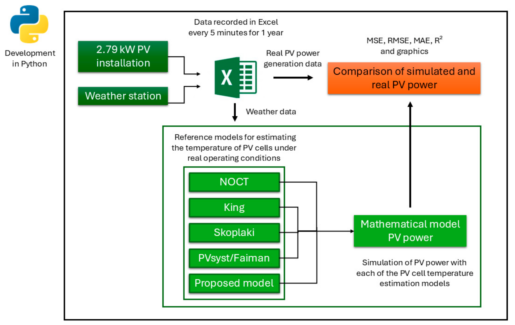
The complete processing, calibration, and validation were implemented in Python 3.11, utilizing NumPy (v1.24) for array operations, Pandas (v2.0) for data management, SciPy (v1.10) for optimization, and Scikit-learn (v1.3) for evaluation metrics. Computational hardware: Intel Core i7-9700K (8 cores, 3.6 GHz), 32 GB DDR4 RAM, and NVIDIA RTX 2060. Code developed in Visual Studio Code v.1.117 and available on GitHub 2026 https://github.com/Dorotea93/Physical-model-optimized-by-evolutionary-algorithms-for-the-accurate-estimation-of-cell-temperature- (accessed on 31 July 2025). Figure 2 shows an outline of the working methodology developed in this article.

2.2. Reference Models

The four reference models were implemented in Python using the exact mathematical formulations from the scientific literature shown below. The parameters of each model were extracted from the manufacturer’s specifications and standard literature values, without applying local recalibration to site-specific conditions. In contrast, the proposed model was specifically calibrated to the local climatic conditions of Badajoz by means of the differential evolution algorithm, allowing a rigorous comparison between a classical approach (fixed parameters) and an adaptive approach (optimized parameters). All models were evaluated on identical data sets (9316 records, uniform pre-processing, identical metrics: R2, RMSE, MSE and MAE), guaranteeing an unbiased and fair comparative analysis.
This section briefly describes the classic NOCT, King, Skoplaki, and PVsyst/Faiman models analyzed in this study to estimate the photovoltaic cell temperature (see Table 2). To determine the installation’s PV power output based on these temperature estimates, we use the calculation model described in [36].
  • NOCT model (Nominal Operating Cell Temperature): This model estimates the cell temperature (Tc) from the ambient temperature, irradiance and the NOCT value provided by the manufacturer. Standard wind conditions (generally 1 m/s) and a reference irradiance of 800 W/m2 are assumed. Where NOCT is the nominal operating temperature of the cell, depending on the panel technology specified in the panel’s data sheet (in our case study, it is 45 °C), Tamb is the ambient temperature, and G is the irradiance value measured on the same inclined plane as the PV panel [20].
  • King model: In the equation proposed by King, the parameters a and b represent the influence of solar radiation and wind speed on the panel temperature, respectively. The TSR0 variable corresponds to the solar radiation received on the inclined surface of the panel, adjusted for the model as normalized inclined radiation. In the specific case of a flat plate array, the values assigned to these coefficients are a equal to 3.473 and b equal to 0.0594 s m−1 and w is the wind speed [37].
  • Skoplaki model: The direct solar irradiance on the inclined surface of the panel is expressed as G. For standard operating conditions (NOCT), the reference irradiance is TSRNOCT = 800 W/m2, the nominal operating temperature of the cell is TNOCT = 45 °C, and the ambient temperature under these conditions is Tamb,NOCT = 20 °C. The convective heat transfer coefficient under NOCT conditions is hw,NOCT = 10.91 W/m2K. Regarding the optical and electrical parameters of the module, an absorbed radiation fraction (τα) of 0.9, an efficiency (η) of 0.12 and a temperature coefficient of efficiency (μ) of 0.00048 °C were used. Finally, the wind convection heat transfer coefficient, hw, was calculated based on wind speed according to the expression, hw = 8.91 + 2.0 [37].
  • PVsyst/Faiman model: PVsyst software, widely used for modelling the performance of photovoltaic systems, uses a temperature model based on Faiman’s formulation. This model estimates the cell temperature from the ambient temperature, solar irradiance, solar absorptance of the module (α), reference efficiency of the module ηref and two heat transfer coefficients, U0 and U1, which represent heat dissipation by convection and radiation. The values for outdoor installations are 29 W/m2 and 0 W/m3sK, respectively [38].
  • Model for calculating PV power: The model described in [36] (see Equation (1)) allows the calculation of the photovoltaic power generated by a module as a function of the solar irradiance incident on the same inclined plane of the panel, ID, and the photovoltaic cell temperature, TC. Where PMPP is the maximum power of the panel under STC (Standard Test Conditions), and the power loss coefficient due to temperature is represented by β. Finally, to obtain the photovoltaic power of the installation, the power generated by a module, PS’, must be multiplied by the final number of panels installed. It is assumed that the installation company has correctly calculated the cross-section of the photovoltaic cable and that the voltage drop is less than 1.5% according to Spanish instruction ITC-BT 40 [39].
P s = P M P P I D I D r e f   1 β T c T r e f  
The model has been adopted for power estimation due to its extensive validation in real PV systems and its proven accuracy with well-calibrated input variables, such as cell temperature. Its simple formulation allows for rapid computational simulations without compromising the accuracy required for building energy management applications, in line with standard practice in PV software [36].
While it is recognized that the temperature coefficient β may exhibit non-linear behavior under low irradiance conditions, this study adopts the standard linear approach to maintain consistency with existing literature and focuses specifically on the improvements provided by the proposed thermal model.

2.3. Proposed Model

The advanced proposed model for estimating photovoltaic cell temperature (see Equation (2)) is based on a physical model inspired by the NOCT model, but it adds a much more complete and versatile mathematical formula, capable of capturing the thermal dynamics of the modules under real operating conditions with greater realism.
Mathematically, the cell temperature TC[i] at each instant, i, is calculated as the sum of several terms that represent different physical phenomena and environmental effects.
T c i = M o d e l   N O C T i + T h e r m a l   i n e r t i a i + E f f e c t   o f   w i n d i   + C l o u d y   a n d   t r a n s i e n t i + N o n   l i n e a r   t e r m   i + C m e d
The first term corresponds to the classic NOCT structure, which relates the ambient temperature and irradiance to the thermal increase of the cell. However, the model introduces key innovations.
1. Thermal inertia (∆Tiner[i]) is modelled as a weighted sum of the differences between past cell temperatures and the current ambient temperature, allowing the system to have thermal “memory” and respond more realistically to rapid changes in environmental conditions (see Equation (3)). In practice, this mechanism is mathematically represented as a weighted sum of the differences between the cell temperatures recorded at the three previous time points and the current ambient temperature. Each of these differences is multiplied by a specific coefficient (α1, α2 and α3), which determines the relative weight of each past moment in the module’s overall thermal response. In this way, the model can reflect the module’s ability to retain heat and the slow dissipation of accumulated thermal energy, aspects that are particularly relevant in situations of rapid changes in irradiance or wind.
T i n e r i = α 1 T c , i 1 T a m b , i + α 2 T c , i 2 T a m b , i + α 3 T c , i 3 T a m b , i
where ∆Tiner[i] is the thermal inertia correction to be applied at the current moment, and Tc,i−1, Tc,i−2 and Tc,i−3 are the cell temperatures at the three previous moments.
Each term represents the influence of the difference between the cell’s previous temperature and the current ambient temperature on the module’s thermal response. The weighted sum of these terms allows us to model the system’s thermal “memory,” reflecting its inertia in the face of rapid environmental changes.
In the computational formulation of the model, realistic physical limits were imposed on the thermal inertia term for the Badajoz region, restricting it to the range of −50 °C to 50 °C at each calculation. This restriction was implemented using the np.clip function in Python and aims to prevent the propagation of extreme values that do not correspond to the physical reality of the system, thus ensuring the robustness and interpretability of the predictions.
2. The effect of wind (see Equation (4)) is modelled in an advanced way, not only as a linear term, but also including interactions between ambient temperature, wind speed and irradiance variability. In this way, it incorporates terms proportional to the product of wind speed and the temperature difference with respect to the reference, the derivative of irradiance and the square of wind speed, which allows capturing both direct convective cooling and more subtle effects of meteorological variability.
W i n d   e f f e c t   [ i ] = β 1 T a m b [ i ] T r e f w [ i ] + β 2 d G [ i ] w [ i ] + β 3 w [ i ] 2 ( T a m b [ i ] T r e f )
where β1, β2, β3 are automatically calibrated coefficients, and dG[i] is the time derivative of the irradiance at time i.
The physical interpretation of each term is as follows: the first term, β1 multiplied by the difference between the ambient temperature at time i and the reference temperature, and by the wind speed at that same time, reflects the cooling by direct convection. This term modulates the effect of wind according to the temperature difference between the environment and the reference. The second term, β2 multiplied by the time derivative of the irradiance at time i and the wind speed, introduces the interaction between rapid changes in irradiance, such as passing clouds, and the wind, allowing the model to react to unexpected weather variations. Finally, the third term, β3, by the square of the wind speed and the temperature difference between the ambient and reference temperatures, adds a quadratic wind component. This allows capturing the nonlinear and higher-order effects on convective cooling, which are particularly relevant in situations of strong winds.
This advanced formulation allows the model to represent both the direct effect of wind on the module’s thermal dissipation and the more complex interactions between wind, temperature and irradiance variability, providing a more realistic and accurate estimate of the cell temperature under changing environmental conditions.
3. Cloudiness and transients (see Equation (5)) are modelled using advanced variables: the time derivatives of irradiance (first and second), the standard deviation of irradiance in a moving window, and a binary cloud cover indicator that detects situations of high variability and potential cloud passages. These terms, weighted by the coefficients γ1, γ2, and γ3, allow the model to react to rapid changes in irradiance, which are usually the most difficult to capture with traditional models.
C l o u d i n e s s   a n d   t r a n s i e n t i = γ 1 d G [ i ] + γ 2 σ G , 5 [ i ] c l o u d i n d [ i ] + γ 3 d 2 G [ i ] c l o u d i n d
The equation for determining cloudiness and transients is expressed as the weighted sum of three terms: the first corresponds to the product of the calibratable coefficient γ1 and the absolute value of the first temporal derivative of the irradiance at time i, which represents the change in irradiance with respect to the previous time. The second term is the result of multiplying the coefficient γ2 by the standard deviation of the irradiance calculated in a moving window of five samples around time i, by a binary indicator called cloudind[i], which takes the value of one if a cloudiness situation is detected, characterized by high variability and sudden changes in irradiance, and zero otherwise. Finally, the third term consists of the product of γ3, the second time derivative of irradiance representing the acceleration or change in irradiance variation, and the binary indicator cloudind[i]. The coefficients γ1, γ2 and γ3 are calibratable parameters that allow adjusting the relative importance of each component within the equation.
The physical meaning of the terms considered in the model is as follows: the first term, which involves the product of γ1 by the absolute value of the temporal derivative of the irradiance, allows the model to be sensitive to sudden changes in irradiance, such as those that often occur during cloud passage. The second term, represented by γ2 multiplied by the standard deviation of irradiance and a cloud cover indicator, reinforces the model’s response in situations of high variability, emphasizing periods when irradiance fluctuates rapidly. The third term, which involves γ3 and the second time derivative of irradiance together with the same cloud indicator, introduces sensitivity to the acceleration of irradiance changes, allowing the capture of complex transient phenomena.
In the proposed model, the binary indicator cloudind[i] is used to detect moments when solar irradiance experiences sudden variations, a phenomenon generally linked to the passage of clouds or to variable cloudiness conditions. This indicator takes the value of one when a situation of high variability and abrupt change in irradiance is identified, and zero in stable conditions where no significant alterations are observed. For practical calculation, the first-time derivative of irradiance, dG[i], which represents the change from the previous value, is evaluated at each instant, as well as the standard deviation of irradiance in a moving window of five samples, σG,5[i], which quantifies local variability. The indicator is activated, that is, it takes the value of one, only when the absolute change in irradiance exceeds 50 W/m2 and the local standard deviation is greater than 100 W/m2, which allows distinguishing relevant cloudy situations from stable conditions. This logic, implemented in Python code, facilitates the automatic identification of transient cloud events in irradiance time series, improving the model’s sensitivity to rapid and complex fluctuations.
Experimental validation shows that cloud_indicator is activated 14.60% of the time (1360 of 9316 observations). These thresholds are located at the 75th percentile of their respective distributions, guaranteeing the detection of essentially significant transient events. The parameters γ2 and γ3 contribute significantly to the model’s accuracy during cloudy periods.
Taken together, these terms give the model the ability to react to rapid and difficult-to-predict meteorological events, improving cell temperature estimation compared to traditional models that only consider averages or linear relationships.
4. The non-linear term (see Equation (6)), based on the square root of the irradiance multiplied by the temperature difference between ambient and the reference temperatures, introduces additional flexibility to adjust the thermal response under high irradiance conditions, where non-linear effects can be relevant.
δ G i ( T a m b [ i ] T r e f )
where δ is the coefficient that adjusts the weight or importance of the non-linear term in the model, and its value is automatically adjusted during the model optimization process so that the cell temperature prediction is as close as possible to the actual data from the installation.
The inclusion of this non-linear term responds to the need to capture physical phenomena that cannot be adequately described by strict linear relationships, especially under conditions of high irradiance and extreme temperatures.
Physically, heat transfer to the photovoltaic module and its dissipation do not always show a linear dependence on irradiance. In situations of high irradiance, the thermal behavior of the module can be influenced by effects such as convection saturation, non-linear radiative emission and variability in thermal dissipation efficiency, factors that tend to smooth the thermal response to additional increases in irradiance [40]. Therefore, the use of the square root of irradiance in the model reflects this attenuated dependence, avoiding the overestimation of cell temperature that would result from a purely linear term.
On the other hand, multiplication by the temperature difference allows the non-linear effect to be more relevant when the ambient temperature deviates from the reference, i.e., in conditions of extreme heat or cold. In this way, the model can adapt to both very hot days and mild days, adjusting the thermal sensitivity according to the context.
In practice, purely linear models tend to underestimate or overestimate the cell temperature under certain combinations of irradiance and ambient temperature. The non-linear term acts as an “adaptive corrector” that allows the model to learn from actual data and improve the fit in scenarios where physical effects are not strictly proportional.
5. The parameter Cmed is a global correction term that is added to the final equation to adjust the cell temperature prediction, compensating for systematic biases and minimizing errors due to uncertainties or specific conditions. In addition, it improves the statistical fit of the model during calibration, allowing it to adapt to unmodelled factors such as microclimate or module ageing.

2.4. Model Calibration and Validation

For the calibration and evaluation of the proposed model for estimating photovoltaic cell temperature, an approach based on evolutionary optimization, standard statistical metrics and a seasonal comparative procedure was used.
Evolutionary algorithm and objective function
The automatic calibration of the model parameters was carried out using the differential evolution algorithm, implemented using the Python scipy.optimize library: configured with population size (popsize) = 40, maximum iterations (maxiter) = 1000, adaptive mutation factor F in [0.5, 1.0], crossover probability Cr = 0.80, and random seed = 42 to ensure result reproducibility. This evolutionary technique is recognized for its robustness and effectiveness in optimizing non-linear and high-dimensional functions, which are common characteristics of complex physical models [41]. The algorithm explores the parameter search space stochastically, allowing it to avoid local minima and increase the probability of finding the optimal combination of parameters that maximizes the fit of the model to the experimental data.
During the calibration process, all model coefficients (such as α1, α2 and α3 for thermal inertia, β1, β2 and β3 for wind effect, γ1, γ2 and γ3 for cloudiness and transients, as well as the non-linear and global correction terms) allow the model to adapt flexibly to actual operating conditions.
The objective function employed was to maximize the coefficient of determination R2 between the simulated power and the actual measured power. To achieve this, the algorithm minimizes the negative value of R2, directing the calibration towards obtaining the highest possible degree of statistical correlation between the model’s prediction and the observed data. This strategy ensures that the calibration not only seeks to reduce the absolute error but also maximizes the model’s explanatory power with respect to the variability of the actual data.
Convergence was achieved in 400–600 iterations (45–90 s per calibration run) on the specified hardware. K-Fold cross-validation with k = 5 required approximately 7–10 min of real time, representing a negligible computational overhead for the annual calibration cycle.
Evaluation metrics
To evaluate the performance of each model, various statistical metrics were used to quantify the accuracy and predictive power of the simulations with respect to the actual data. Among these, the mean squared error (MSE) is used to measure the average of the squared errors between the estimated power and the actual power, giving greater weight to larger errors. The root mean squared error (RMSE), which is the square root of the MSE and is expressed in the same units as the variable of interest, facilitates the physical interpretation of discrepancies between the model and reality.
For its part, the mean absolute error (MAE) provides a direct measure of accuracy, as it calculates the average of the absolute errors without excessively penalizing outliers, making it particularly useful for comparing the robustness of different approaches. Finally, the coefficient of determination (R2) indicates what proportion of the variability present in the actual data is explained by the model; results close to one reflect an excellent fit between the simulation and reality. The combined use of these metrics allows for an objective and rigorous comparison of the different models analyzed.
Seasonal comparison procedure
To evaluate the adaptability of the different models to the specific conditions of each season, the data were divided according to the four seasons of the year: winter, spring, summer and autumn. For our own model, individual calibration of the parameters was carried out, and the corresponding evaluation metrics were calculated for each season. This approach allowed us to analyze in detail how each model responds to the climatic particularities of each season in the Badajoz region, thus facilitating a more precise and demonstrative comparison of their performance in variable environmental conditions.
Validation Methodology
Model validation was performed using K-Fold cross-validation (K = 5) and temporal validation strategies. K-Fold results demonstrate excellent model generalization: training R2 = 0.8599 ± 0.0021 vs. validation R2 = 0.8572 ± 0.0073 (difference of 0.27%). Temporal validation across seasons yields comparable performance: spring/autumn training R2 = 0.8615 vs. winter validation R2 = 0.8551. The consistency of validation metrics across different datasets confirms that the model generalizes well to unseen data without overfitting. The greater accuracy during summer and autumn reflects lower atmospheric variability in these seasons, resulting in more predictable cell temperature behavior.

3. Results

3.1. Calibration and Optimal Parameters

The calibration of the model developed was carried out through an automatic optimization process using the differential evolution algorithm, which allowed all the model coefficients to be simultaneously adjusted to the experimental data of the photovoltaic installation. This procedure was applied to each season independently, with the aim of capturing seasonal variability and maximizing predictive capacity under different environmental conditions. During calibration, the parameters associated with the different modelled physical phenomena were optimized: thermal inertia α1, α2 and α3, wind effect β1, β2 and β3, cloudiness and transients (γ1, γ2 and γ3), the non-linear term (δ) and the global correction term (Cmed). The objective function used was the maximization of the coefficient of determination (R2) between the simulated and measured power, which guarantees an optimal statistical fit.
Table 3 shows the optimal values obtained for each parameter after seasonal calibration. These results allow us to analyze the relative influence of each phenomenon on the thermal behavior of the system, as well as to identify possible differences in the model’s response depending on the season of the year. It should be noted that some parameters have zero values in certain seasons, indicating that the optimizer considered their contribution to be insignificant under those conditions. The variability observed in the parameters between seasons reflects the model’s ability to adapt to the climatic particularities of each period.

3.2. Interpretation of Seasonal Variability in Optimal Parameters

The presence of zero or practically negligible parameters in certain stations, such as α2 and α3 in most periods, β3 in summer, γ1 and γ2 in autumn, or δ in spring and summer, demonstrates that the physical phenomena they represent do not significantly improve the model’s fit under those specific climatic conditions. This situation can be explained by several reasons. First, it could be due to redundancy; that is, the corresponding physical effect is already adequately accounted for in other terms of the model, making its explicit contribution unnecessary. Second, in summer, since irradiance barely varies, the phenomena associated with rapid fluctuations in solar radiation have very little influence on cell temperature. Therefore, the model does not need to consider these effects to make accurate predictions. Finally, by automatically adjusting the model, this process eliminates terms that do not provide useful information for improving predictions and, consequently, avoids unnecessary complications. As a result, the model remains simple and robust, adapting to the conditions of each season and using only the physical factors that actually influence each situation.
Next, we analyze in detail the behavior and relevance of each of the parameters calculated in the model, delving into their physical interpretation and the influence they exert under different seasonal conditions.
  • Thermal inertia
The analysis of the thermal inertia coefficients (α1, α2 and α3) reveals that the parameter α1 reaches high values in spring (0.61) and summer (0.62), highlighting the importance of the thermal memory of the photovoltaic module during these seasons, which are characterized by greater variability in both irradiance and temperature. In winter, α1 also has a significant value (0.50), although notably lower than in spring and summer, while in autumn it drops sharply to 0.17, reflecting a lower influence of thermal inertia under more stable conditions. On the other hand, the coefficients α2 and α3 are zero or practically negligible in most seasons, with the sole exception of α2 in autumn (0.035), suggesting that the contribution of second- and third-order thermal memories is, in general, irrelevant or redundant. Only in autumn, when thermal transitions are smoother, is a slight additional influence of these terms detected.
The analysis of the parameters associated with the wind effect shows clear seasonal variability in its influence on the thermal dissipation of the photovoltaic system. The coefficient β1 reaches its maximum value in spring (0.12), followed by autumn (0.08), indicating that wind-induced convective cooling is particularly relevant in these periods, characterized by higher wind frequency and intensity. Conversely, in summer and winter, the value of β1 decreases significantly, reflecting the lower incidence of wind on thermal dissipation under conditions of extreme heat or atmospheric stability. It is important to note that in regions like Badajoz, during the summer, the average wind speed is usually considerably low, which further limits the effect of wind on cell temperature and explains the reduced or even zero values of the coefficients related to this phenomenon in that season.
  • Effect of wind
As for β2, it is observed that it maintains positive and similar values during winter, spring and summer, suggesting a constant contribution of the interaction between wind and irradiance variability in the thermal response of the module. However, in autumn this coefficient becomes negative (−0.007), which could be interpreted as a compensatory effect or a lower relevance of this interaction under the weather conditions typical of that season.
Finally, the β3 parameter is zero in summer and becomes more relevant in spring and autumn. In summer, atmospheric stability and low wind speeds reduce their impact on the thermal behavior of the system, making these terms irrelevant in the modelling for that season.
  • Cloudiness and transients
The analysis of the coefficients associated with cloudiness and transient phenomena reveals a clear seasonal behavior in the model’s sensitivity to rapid variations in irradiance. The parameter γ1 is relevant in winter and summer, while it is zero in spring and autumn. This indicates that sensitivity to the first derivative of irradiance, i.e., to rapid changes in solar radiation, is particularly important under extreme conditions, such as those prevailing in the coldest and hottest months of the year, but loses significance during the transition seasons, when the atmosphere is usually more stable.
For its part, γ2 reaches its maximum value in spring (0.046) and remains significant in summer, highlighting the influence of local irradiance variability in these periods, characterized by a higher frequency of meteorological events that generate short-term fluctuations in solar radiation.
As for γ3, it is practically zero in summer, low in spring and winter, and reaches its maximum in autumn (0.06). This behavior suggests that the model’s sensitivity to the second derivative of irradiation, i.e., to rapid or sudden changes, only becomes relevant under variable cloud cover conditions typical of autumn, when rapid transitions in solar radiation are more frequent and mark the thermal dynamics of the photovoltaic system.
  • Non-linear term and global correction term
The analysis of the coefficients associated with the non-linear term and the global correction of the model reveals interesting patterns depending on the season. The parameter δ is significant only in winter (0.04) and autumn (0.007), indicating that the non-linear effects derived from the interaction between irradiance and ambient temperature become more important for adjusting the thermal response of the system under cold or transitional conditions. In these seasons, the presence of extreme phenomena or greater atmospheric variability makes it necessary to introduce this term to improve the accuracy of the model, while in spring and summer its contribution is negligible due to greater climatic stability.
The global correction coefficient Cmed, on the other hand, exhibits negative values in all seasons, reaching its maximum magnitude in summer and spring. This behavior can be interpreted as systematic compensation implemented by the model to correct possible biases associated with extreme irradiance or temperature conditions, especially in the warmest and sunniest periods of the year. Thus, Cmed acts as an additional adjustment that allows for refining the prediction of cell temperature in the face of factors not explicitly modelled, ensuring greater robustness and reliability in the estimates under diverse environmental scenarios.

3.3. Seasonal Performance Comparison

This section presents and analyses the results of the seasonal comparison between the proposed ultra-enhanced model and the classic reference models (NOCT, King, Skoplaki and PVsyst/Faiman), using the RMSE, MAE and R2 determination coefficient error metrics as the main criteria. The objective is to evaluate the predictive capacity of each model under different climatic conditions and highlight the advantages of the proposed approach over traditional alternatives.
Recent literature validates the superiority of models that integrate dynamic variables. For example, ref. [42] demonstrates that the inclusion of wind speed and thermal inertia in Sandia-type models significantly improves predictive accuracy (RMSE < 3 K), systematically outperforming static models based solely on irradiance and ambient temperature. Advanced approaches, such as transient temperature models incorporating thermal mass as proposed by [43], achieve RMSE of approximately 1.63 K under general conditions and 3.33 K under rapid transient conditions, representing significant improvements over the standard Faiman model. In comparison, empirical steady-state models exhibit maximum errors of 27 K during rapid irradiance changes, while dynamic models reduce this error to approximately 9 K by capturing the effects of thermal inertia [44].
Table 4 presents the performance metrics obtained by each model in the different seasons of the year, considering the characteristic climate variability of Badajoz.
Throughout all seasons of the year, the proposed model stands out for consistently offering the highest R2 values and the lowest RMSE and MAE values compared to classic models. This superiority is clearly reflected in the direct comparison with the best classic model for each season. For example, in winter, the model achieves an R2 of 0.8628, which is an improvement of 0.86% over the King model, which is the best-performing classic model for that season. In spring, the R2 obtained is 0.7743, exceeding the NOCT model by 0.25%. During summer, the proposed model achieves an R2 of 0.9055, representing an improvement of 1.11% over the King model. Finally, in autumn, the proposed model achieves an R2 of 0.9236, improving on the King model by 0.51%.
In terms of errors, it should be noted that the proposed model manages to reduce the RMSE in all seasons. For example, in summer, the RMSE decreases by 4.9% compared to the King model (0.2773 vs. 0.2915), while in autumn the reduction is 2.9% (0.2172 vs. 0.2237). Similarly, the MAE is consistently lower with the proposed model: in summer, there is a reduction of 14.4% compared to the King model (0.1223 vs. 0.1429), and in autumn, the decrease reaches 4.6% (0.0996 vs. 0.1045).
The experimental reliability of the comparative analysis was assessed by calculating the combined standard uncertainty (uc) according to the ISO/IEC Guide 98-3 (GUM) [45]. This approach employs the Root Sum of Squares (RSS) method to propagate the individual Type B uncertainties of the measuring equipment. This value integrates the individual accuracies identified in Table 1: solar radiation, DC power monitoring, and the secondary influence of ambient temperature and wind speed sensors. The resulting combined uncertainty of 5.2% (shown in Table 4) serves as a benchmark for the model validation. A model’s performance is considered high-fidelity when its Root Mean Square Error (RMSE) remains within or close to this instrumental uncertainty threshold, indicating that the remaining error is primarily limited by the physical constraints of the sensors.
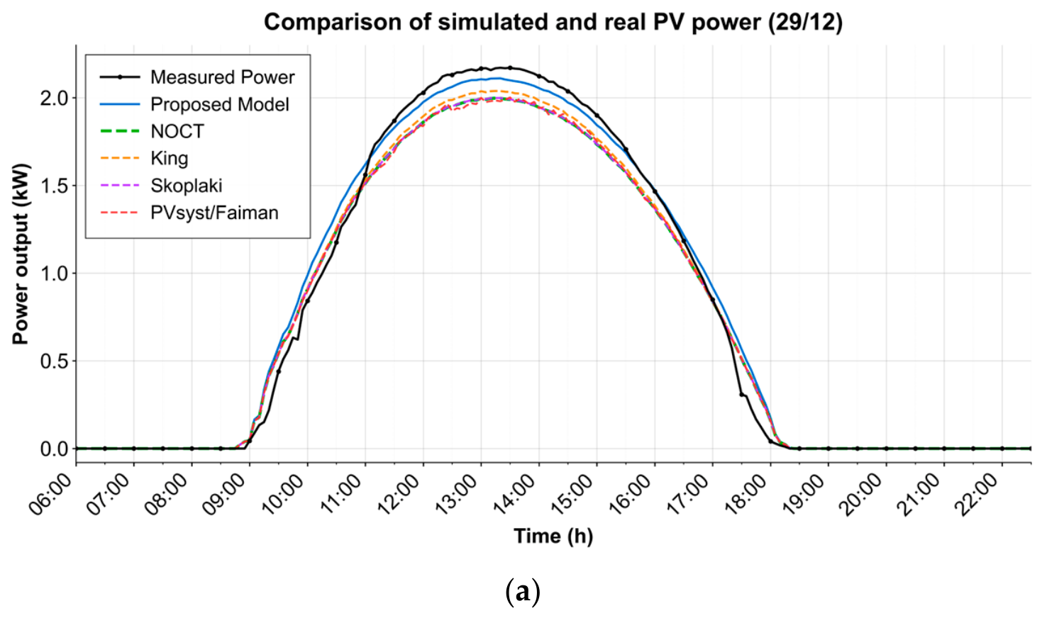
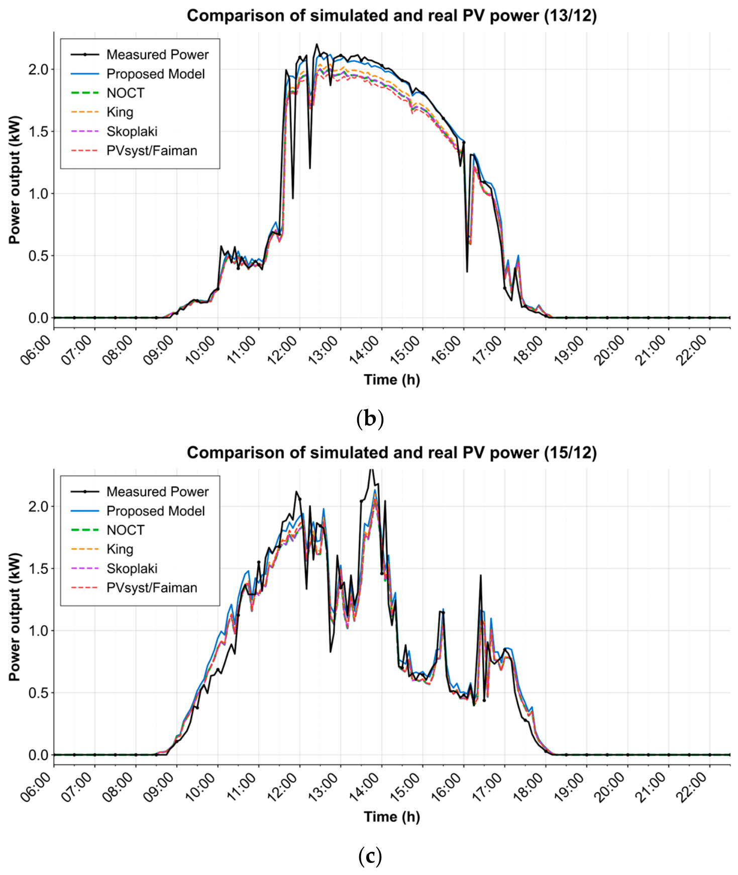
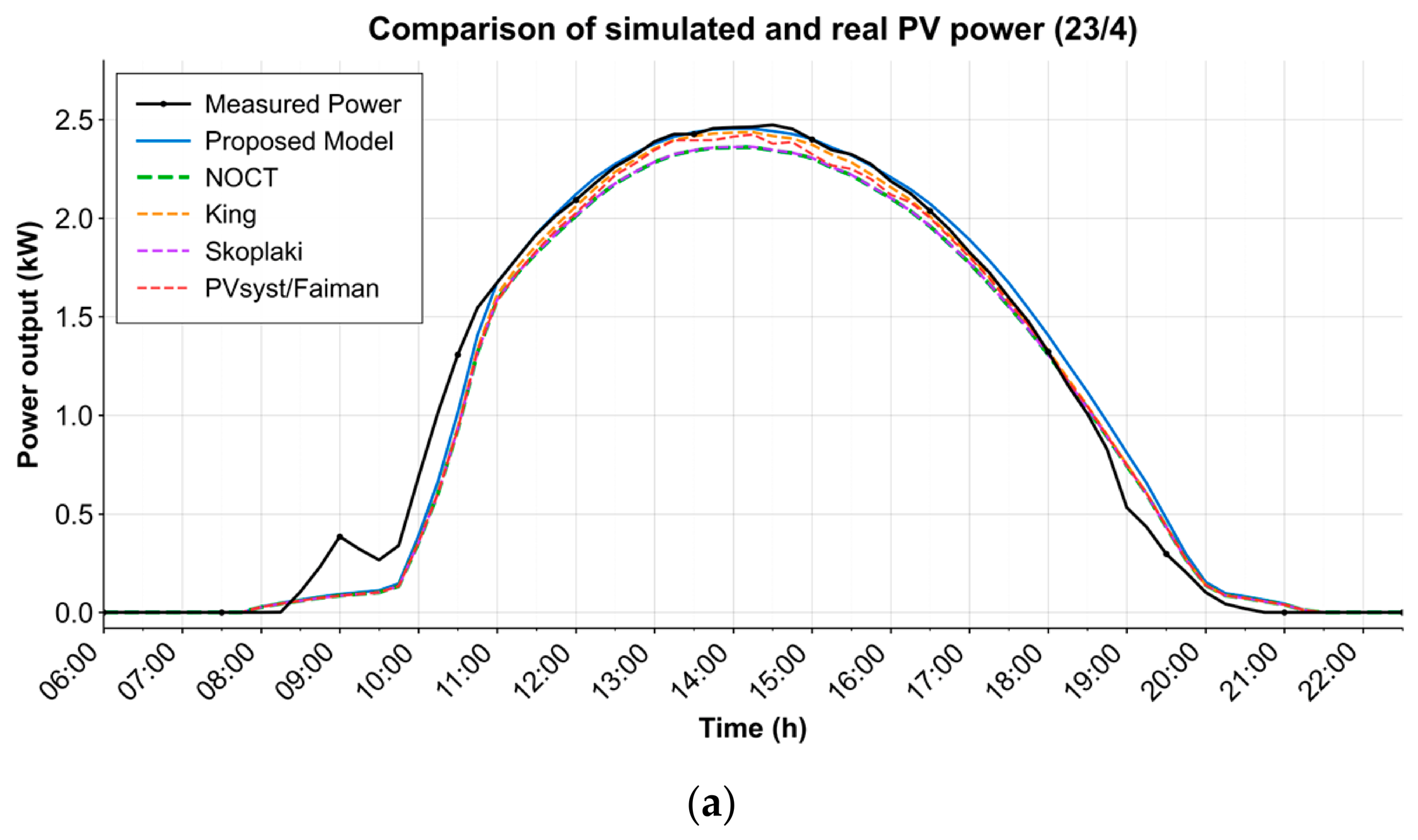
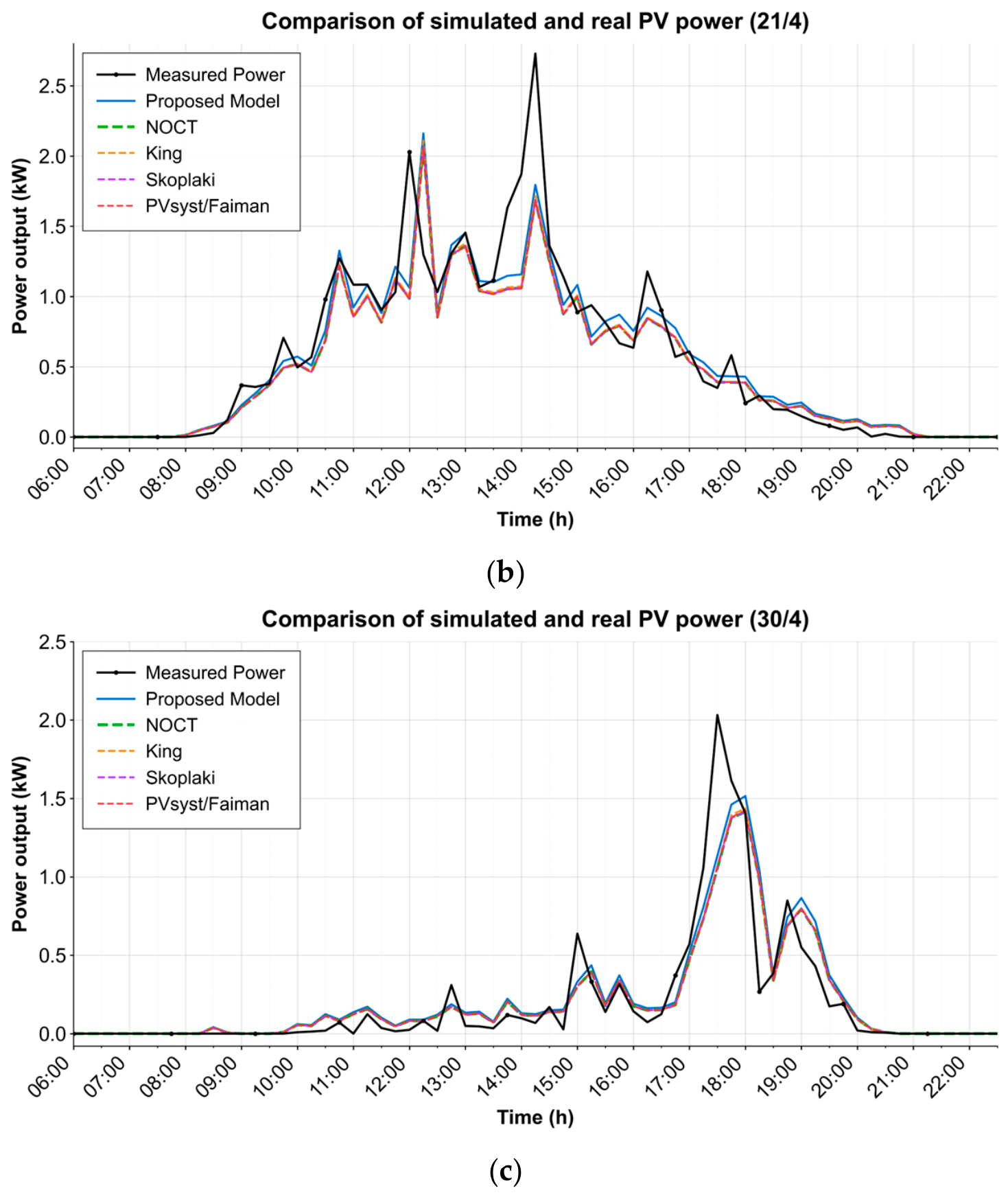
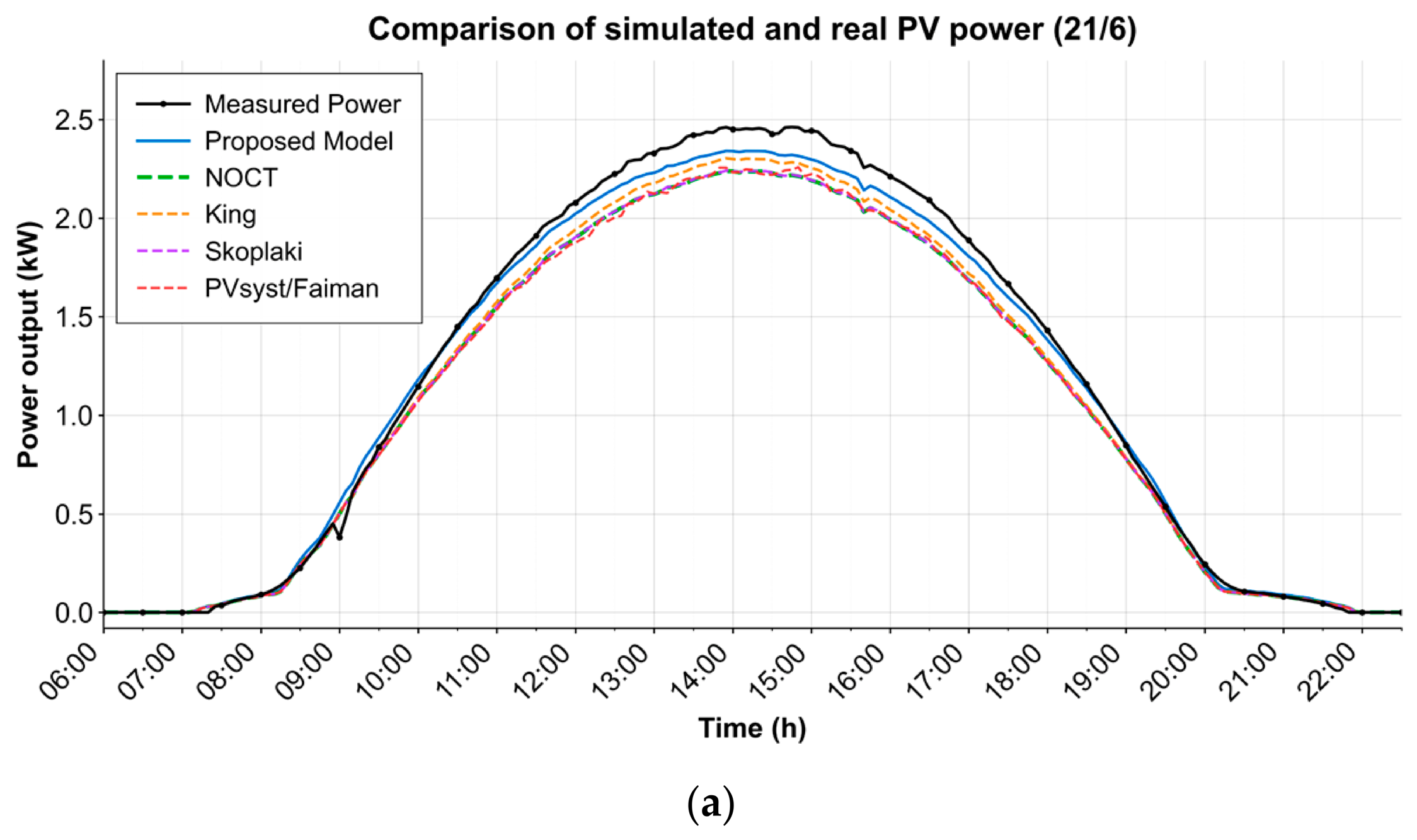
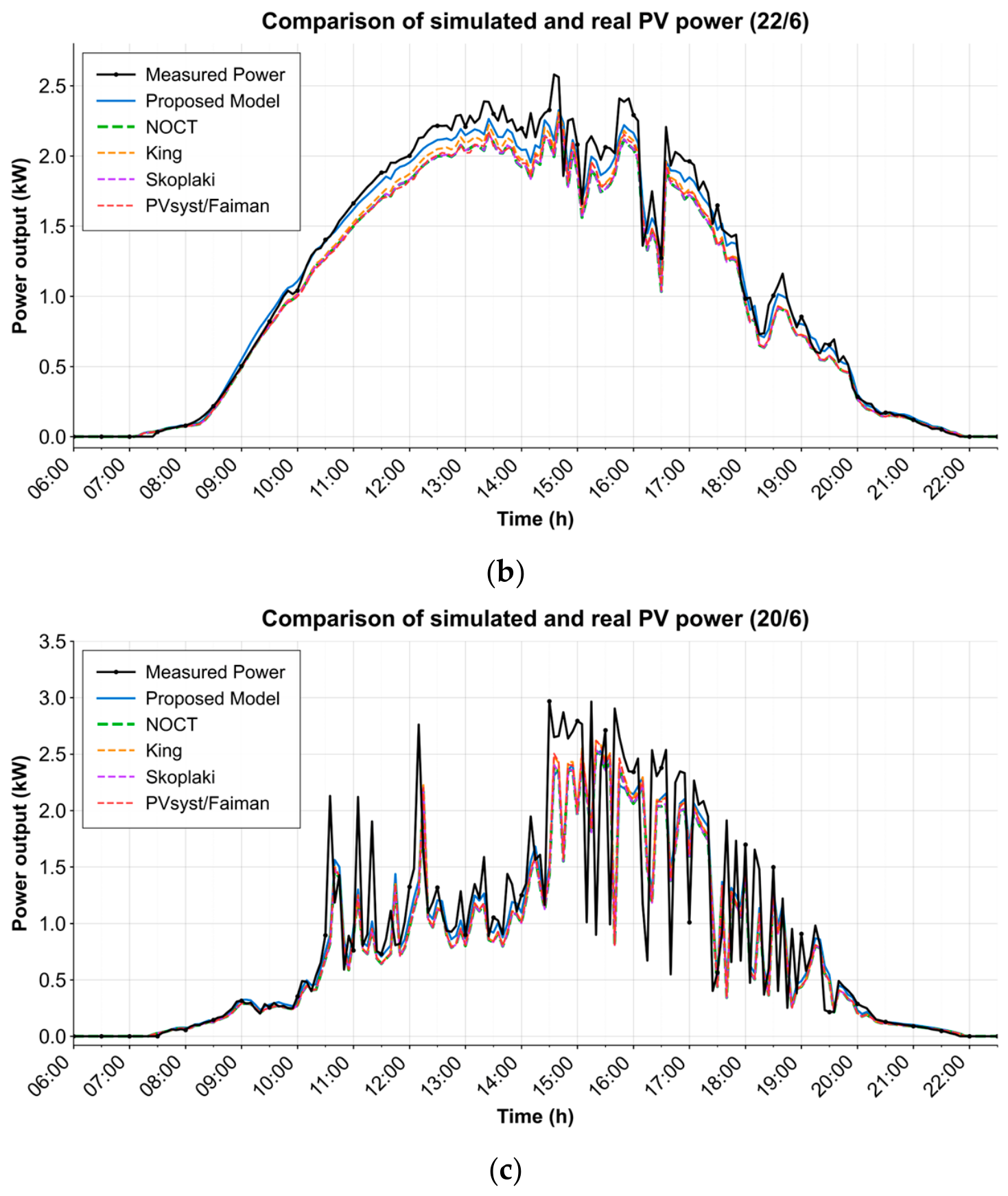
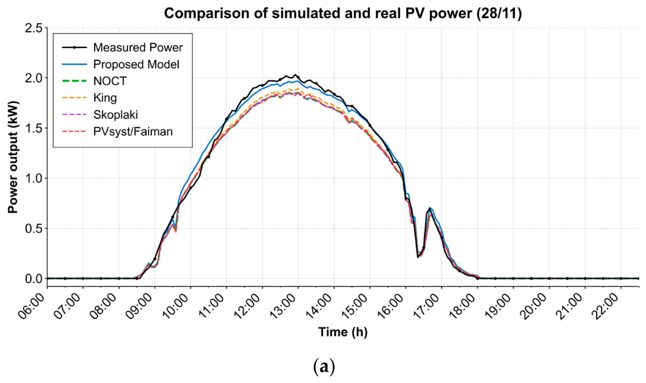
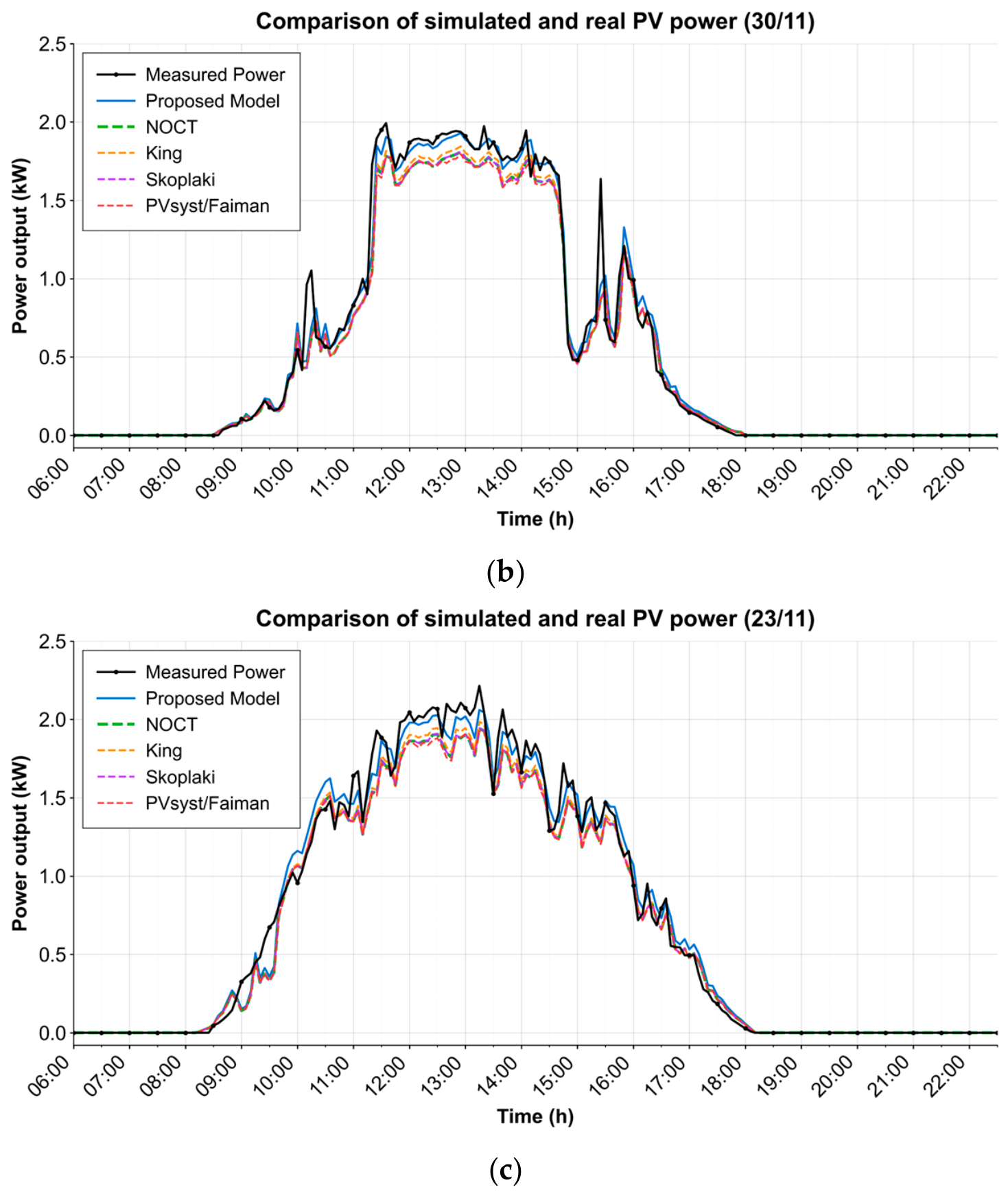
Figure 3, Figure 4, Figure 5 and Figure 6 show the temporal comparison between the actual power and the power simulated by the own model and the reference models (NOCT, King, Skoplaki and PVsyst/Faiman) for different representative days (clear, partly cloudy and cloudy days) in winter, spring, summer and autumn, respectively.
In the visual analysis of the power curves presented in Figure 3, Figure 4, Figure 5 and Figure 6, characteristic patterns can be observed according to the type of day (clear, partly cloudy and cloudy) and the season of the year. On clear days, all models accurately reproduce the general power profile, with a gradual increase until midday, followed by a decrease. However, the proposed model stands out for its greater accuracy during the middle of the day, better matching peak power values and showing less dispersion compared to the actual measurement.
On partly cloudy and cloudy days, the difference between models becomes more evident. Classic models tend to smooth out the response to rapid irradiance variations, resulting in an underestimation of power peaks and a delay in recovery after clouds cover. For example, in Figure 3b (winter and partly cloudy day), it can be seen how the classical models fail to adequately capture the sudden increases and decreases in power that occur between 12:00 and 14:00, while the proposed model more accurately reproduces the actual dynamics, correcting both the magnitude and timing of the peaks.
Similarly, in Figure 4c (spring and cloudy day), meteorological events where irradiance varies rapidly are identified. In these cases, the model responds with greater sensitivity and speed, avoiding the time lag exhibited by classical models. This behavior is repeated in summer and autumn, where the advanced model maintains a greater capacity to adapt to atmospheric variability, especially in the early afternoon, when the most abrupt changes in irradiance tend to occur.
These results demonstrate that incorporating specific terms for thermal inertia and irradiance variability in the proposed model allows for a more realistic and robust response to high variability situations, improving the prediction of power generated in complex scenarios.

4. Discussion

Practical applicability of the proposed model
The implementation of the advanced photovoltaic cell temperature estimation model developed in this work offers tangible advantages for the energy management of solar systems in buildings. The greater accuracy achieved in cell temperature prediction translates directly into a more reliable estimate of the power generated, allowing for more accurate anticipation of the daily and seasonal production of the photovoltaic system. This improvement in predictive capability facilitates the optimization of self-consumption strategies, as it enables more efficient programming of energy demand and the use of storage systems, maximizing the use of available solar energy.
Furthermore, the model’s robustness and sensitivity to rapid variations in irradiance and changes in weather conditions allow for the early detection of potential system anomalies, such as performance losses due to dirt, shading, or module failures. This early diagnostic capability contributes to proactive maintenance management and reduced downtime, improving the reliability and profitability of the photovoltaic installation.
In a broader context, the integration of this model into digital twin platforms or advanced monitoring systems can provide significant added value by offering accurate, real-time information for decision-making regarding the operation, maintenance and energy planning of smart buildings.
Statistical significance and practical value of improvements
While the improvements observed in R2 (0.25–1.11%) might seem marginal from a global statistical perspective, their practical impact is significant when analyzing the reduction in residual errors during critical operating periods. A comparative analysis of residuals between the proposed model and the best classical alternative reveals that the largest deviations in the classical models occur during rapid irradiance transients and periods of high thermal stress (summer). In these specific scenarios, our model reduces peak errors by up to 4.9% (RMSE).
From a practical and economic standpoint, this reduction in error is non-negligible for Digital Twin applications. It is widely recognized that a temperature estimation error of 1 °C can lead to a power prediction error of approximately 0.4% to 0.5%. This is consistent with the typical temperature coefficients β for crystalline silicon modules reported in the literature [46]. Therefore, the 14.4% reduction in MAE achieved in summer translates directly into a more accurate power forecast. This accuracy is crucial for:
  • Minimizing imbalance penalties in intraday electricity markets, where deviations between scheduled and actual delivery are penalized [47].
  • Early fault detection, as the model effectively distinguishes between normal thermal transients and current anomalies (e.g., hotspots or dirt), reducing false positives in maintenance alerts [48].
Therefore, the value of the proposed model lies not only in the average annual improvement but in its superior reliability during the most demanding and financially sensitive operating periods.
Limitations and possible areas for improvement
Despite the satisfactory results obtained, the model has certain limitations that should be considered. Its performance depends largely on the quality and representativeness of the data used during calibration. Thus, extreme weather conditions, such as heat waves, intense storms, or episodes of Saharan dust, may not be adequately reflected in the current database, which could affect the accuracy of the model under these less frequent scenarios.
Furthermore, although the model incorporates advanced terms to capture rapid variability in irradiance and non-linear effects, there are other external factors that are not explicitly modelled, such as module ageing, dirt accumulation and the impact of partial shading, which can also influence cell temperature and power output.
Regarding future lines of work, it would be of particular interest to apply and validate the model in other facilities located in different climatic contexts, especially in regions with extreme or highly variable conditions. Expanding the experimental database to include records from additional years and exceptional weather events would strengthen the results and allow for analysis of the model’s behavior in even more complex scenarios. Furthermore, exploring the integration of complementary sensors (for example, to quantify soiling or shading) and analyzing the model’s adaptation to different photovoltaic technologies and geographical locations will be key steps to increasing its versatility and applicability. Finally, combining the model with machine learning techniques to optimize real-time calibration could open new avenues for improvement, enabling greater robustness and reliability in prediction under diverse operating conditions.

5. Conclusions

This work presents the development, calibration, and validation of an advanced physical model for estimating photovoltaic cell temperature, optimized via evolutionary algorithms (Differential Evolution). By incorporating terms for thermal inertia, non-linear wind interactions, and rapid irradiance transients, the proposed model successfully addresses the limitations of classical static approaches.
The experimental validation, conducted over a full year in a pilot installation, quantitatively demonstrates the superiority of the proposed model over standard reference models (NOCT, King, Skoplaki, and PVsyst/Faiman) across all seasons. The most significant improvements were observed during periods of high thermal stress and variability:
  • In Summer, the model achieved a reduction in Root Mean Square Error (RMSE) of 4.9% and a decrease in Mean Absolute Error (MAE) of 14.4% compared to the best-performing classical model (King). The coefficient of determination (R2) reached 0.9055, representing an improvement of 1.11%.
  • In Autumn, the model maintained its robustness with a 2.9% reduction in RMSE and a 4.6% reduction in MAE, achieving the highest accuracy of the year with an R2 of 0.9236.
  • In Winter and Spring, the model consistently outperformed the references, improving R2 by 0.86% and 0.25%, respectively, compared to the best alternatives for those seasons.
These quantitative results confirm that the automatic calibration of physical parameters (specifically those governing thermal memory and transient responses) significantly reduces prediction errors. This accuracy is fundamental for the development of high-fidelity Digital Twins, enabling more precise power generation forecasting and the early detection of operational anomalies (such as soiling or shading) that static models might misinterpret as normal thermal variations.
Consequently, the proposed methodology offers a versatile and transferable tool for researchers and engineers. Future work will focus on validating this approach in diverse climatic zones and integrating machine learning techniques to further refine real-time adaptability.

Author Contributions

Conceptualization, J.F.G.G., D.D.-A. and D.C.F.; methodology, D.D.-A. and D.C.F.; software, J.A.Á.M.; validation, J.F.G.G., D.D.-A. and D.C.F.; formal analysis, M.C.G.; investigation, D.D.-A. and D.C.F.; resources, J.F.G.G. and D.C.F.; data curation, J.F.G.G., D.D.-A. and D.C.F.; writing—original draft preparation, J.F.G.G. and D.D.-A.; writing—review and editing, J.A.Á.M. and M.C.G.; visualization, D.D.-A. and D.C.F.; supervision, J.F.G.G. and D.C.F.; project administration, J.F.G.G.; funding acquisition, J.F.G.G. and D.C.F. All authors have read and agreed to the published version of the manuscript.

Funding

This research was funded by Project TED2021-132326B-I00, Strategic Projects Oriented to the “Ecological Transition and Digital Transition”, funded by MCIN/AEI/10.13039/501100011033 and by the European Union NextGenerationEU/PRTR.

Data Availability Statement

Acknowledgments

The authors thank the RIMSGES network (RED for Research in Sustainable Energy Management Models) of the CYTED programme for the support received in the doctoral thesis of the author D.D.-A. This work was (partially) supported by Programa Iberoamericano de Ciencia y Tecnología para el Desarrollo—CYTED (through Red RIMSGES).

Conflicts of Interest

The authors declare no conflicts of interest.

Abbreviations

The following abbreviations are used in this manuscript:
Tc[i]Cell temperature at time i.
CmedGlobal correction term to adjust the temperature prediction.
α1, α2, α3Weighting coefficients for thermal inertia.
β1, β2, β3Calibrated coefficients for wind effect.
γ1, γ2, γ3Calibrated coefficients for cloudiness and transients.
δCoefficient for the non-linear term.
Tamb [i]Ambient temperature at time i.
TrefReference temperature established in the datasheet, below which the electrical parameters of the photovoltaic panel are determined.
w[i]Wind speed at time i.
dG[i]Temporal derivative of irradiance at time i.
cloudind[i]Binary cloud indicator at time i.
σG,5[i]Standard deviation of irradiance in a moving window of 5 samples at time i.
G[i]Solar irradiance at time i.
PMPPMaximum power of the module under standard conditions.
IDSolar irradiance incident on the inclined plane of the panel.
IDrefReference solar irradiance.
βPower loss coefficient due to temperature.
TambAmbient temperature.
αSolar absorptance of the module.
ηrefReference efficiency of the module.
U0Convective heat transfer coefficient.
U1Radiation heat transfer coefficient.

References

  1. European Parliament European Green Pact: Key to a Climate-Neutral and Sustainable EU. Available online: https://www.europarl.europa.eu/topics/es/article/20200618STO81513/pacto-verde-europeo-clave-para-una-ue-climaticamente-neutral-y-sostenible (accessed on 22 April 2025).
  2. European Parliament Energy Efficiency of Buildings: New Law to Decarbonise the Sector. Available online: https://www.europarl.europa.eu/news/es/press-room/20240308IPR19003/eficiencia-energetica-de-los-edificios-nueva-ley-para-descarbonizar-el-sector (accessed on 22 April 2025).
  3. Hong, J.; Wu, H.; Wu, H.; Li, K.; Wang, D.; Shrestha, A. How Technology Convergence Drives the Invention of Carbon-Neutral Building Technologies? Investigation through the Lens of Binary Innovation Theory. Build. Environ. 2025, 271, 112623. [Google Scholar] [CrossRef]
  4. Wirtz, W.; Meyer, K.; Brendel, R.; Schulte-Huxel, H. Improved Robustness Against Thermal Stress for Building-Integrated PV Modules Built on Aluminum Façade Elements. Prog. Photovolt. Res. Appl. 2025, 33, 717–725. [Google Scholar] [CrossRef]
  5. Stolz, P.; Frischknecht, R.; Kessler, T.; Züger, Y. Life Cycle Assessment of PV-Battery Systems for a Cloakroom and Club Building in Zurich. Prog. Photovolt. Res. Appl. 2019, 27, 926–933. [Google Scholar] [CrossRef]
  6. Mollineda, L.G.F.; García, J.R.A. Digital twin of a photovoltaic system. J. Eng. Technol. Ind. Appl. 2024, 10, 159–171. [Google Scholar] [CrossRef]
  7. Hohm, D.P.; Ropp, M.E. Comparative Study of Maximum Power Point Tracking Algorithms. Prog. Photovolt. Res. Appl. 2003, 11, 47–62. [Google Scholar] [CrossRef]
  8. Ebhota, W.S.; Tabakov, P.Y. Influence of Photovoltaic Cell Technologies and Elevated Temperature on Photovoltaic System Performance. Ain Shams Eng. J. 2023, 14, 101984. [Google Scholar] [CrossRef]
  9. Yu, T.; Ren, C.; Jia, Y.; Li, J.; Zhang, J.; Xu, Y.; Yan, B.; Zhang, M.; Qiao, L.; Wang, T.; et al. Photovoltaic Panel Temperature Monitoring and Prediction by Raman Distributed Temperature Sensor with Fuzzy Temperature Difference Threshold Method. IEEE Sens. J. 2021, 21, 373–380. [Google Scholar] [CrossRef]
  10. Santiago, I.; Trillo-Montero, D.; Moreno-Garcia, I.M.; Pallarés-López, V.; Luna-Rodríguez, J.J. Modeling of Photovoltaic Cell Temperature Losses: A Review and a Practice Case in South Spain. Renew. Sustain. Energy Rev. 2018, 90, 70–89. [Google Scholar] [CrossRef]
  11. Quest, H.; Fairbrother, A.; Ballif, C.; Virtuani, A. Towards a Quantification of Thermal and Thermomechanical Stress for Modules in Building-Integrated Photovoltaics Configurations. Prog. Photovolt. Res. Appl. 2025, 33, 64–75. [Google Scholar] [CrossRef]
  12. Li, G.; Feng, F.; Wang, F.; Wei, B. Temperature Field Measurement of Photovoltaic Module Based on Fiber Bragg Grating Sensor Array. Materials 2022, 15, 5324. [Google Scholar] [CrossRef]
  13. Mavromatakis, F.; Vignola, F.; Marion, B. Low Irradiance Losses of Photovoltaic Modules. Sol. Energy 2017, 157, 496–506. [Google Scholar] [CrossRef]
  14. Perin Gasparin, F.; Detzel Kipper, F.; Schuck de Oliveira, F.; Krenzinger, A. Assessment on the Variation of Temperature Coefficients of Photovoltaic Modules with Solar Irradiance. Sol. Energy 2022, 244, 126–133. [Google Scholar] [CrossRef]
  15. Louwen, A.; de Waal, A.C.; Schropp, R.E.I.; Faaij, A.P.C.; van Sark, W.G.J.H.M. Comprehensive Characterisation and Analysis of PV Module Performance under Real Operating Conditions. Prog. Photovolt. Res. Appl. 2017, 25, 218–232. [Google Scholar] [CrossRef]
  16. Magunov, A.N.; Pylnev, M.A.; Lapshinov, B.A. Spectral Pyrometry of Objects with Unknown Emissivities in a Temperature Range of 400–1200 K. Instrum. Exp. Tech. 2014, 57, 86–90. [Google Scholar] [CrossRef]
  17. Idzkowski, A.; Karasowska, K.; Walendziuk, W. Analysis of Three Small-Scale Photovoltaic Systems Based on Simulation and Measurement Data. Proceedings 2020, 51, 19. [Google Scholar] [CrossRef]
  18. Sun, V.; Asanakham, A.; Deethayat, T.; Kiatsiriroat, T. A New Method for Evaluating Nominal Operating Cell Temperature (NOCT) of Unglazed Photovoltaic Thermal Module. Energy Rep. 2020, 6, 1029–1042. [Google Scholar] [CrossRef]
  19. Mehdi, M.; Ammari, N.; Alami Merrouni, A.; Benazzouz, A.; Dahmani, M. Experimental Investigation on the Effect of Wind as a Natural Cooling Agent for Photovoltaic Power Plants in Desert Locations. Case Stud. Therm. Eng. 2023, 47, 103038. [Google Scholar] [CrossRef]
  20. Idzkowski, A.; Karasowska, K.; Walendziuk, W. Temperature Analysis of the Stand-Alone and Building Integrated Photovoltaic Systems Based on Simulation and Measurement Data. Energies 2020, 13, 4274. [Google Scholar] [CrossRef]
  21. Umoette, A.T.; Ubom, E.A.; Akpan, I.E. Comparative Analysis of Three NOCT-Based Cell Temperature Models. Int. J. Syst. Sci. Appl. Math. 2016, 1, 69–75. [Google Scholar] [CrossRef]
  22. Tahir, Z.R.; Kanwal, A.; Asim, M.; Bilal, M.; Abdullah, M.; Saleem, S.; Mujtaba, M.A.; Veza, I.; Mousa, M.; Kalam, M.A. Effect of Temperature and Wind Speed on Efficiency of Five Photovoltaic Module Technologies for Different Climatic Zones. Sustainability 2022, 14, 15810. [Google Scholar] [CrossRef]
  23. Martín-Chivelet, N.; Polo, J.; Sanz-Saiz, C.; Núñez Benítez, L.T.; Alonso-Abella, M.; Cuenca, J. Assessment of PV Module Temperature Models for Building-Integrated Photovoltaics (BIPV). Sustainability 2022, 14, 1500. [Google Scholar] [CrossRef]
  24. Barry, J.; Böttcher, D.; Pfeilsticker, K.; Herman-Czezuch, A.; Kimiaie, N.; Meilinger, S.; Schirrmeister, C.; Deneke, H.; Witthuhn, J.; Gödde, F. Dynamic Model of Photovoltaic Module Temperature as a Function of Atmospheric Conditions. Proc. Adv. Sci. Res. 2020, 17, 165–173. [Google Scholar] [CrossRef]
  25. Driesse, A.; Theristis, M.; Stein, J.S. PV Module Operating Temperature Model Equivalence and Parameter Translation. In Proceedings of the Conference Record of the IEEE Photovoltaic Specialists Conference; IEEE: New York, NY, USA, 2022; pp. 172–177. [Google Scholar]
  26. Prilliman, M.; Stein, J.S.; Riley, D.; Tamizhmani, G. Transient Weighted Moving-Average Model of Photovoltaic Module Back-Surface Temperature. IEEE J. Photovolt. 2020, 10, 1053–1060. [Google Scholar] [CrossRef]
  27. Zhan, Z.H.; Shi, L.; Tan, K.C.; Zhang, J. A Survey on Evolutionary Computation for Complex Continuous Optimization. Artif. Intell. Rev. 2022, 55, 59–110. [Google Scholar] [CrossRef]
  28. Maier, H.R.; Razavi, S.; Kapelan, Z.; Matott, L.S.; Kasprzyk, J.; Tolson, B.A. Introductory Overview: Optimization Using Evolutionary Algorithms and Other Metaheuristics. Environ. Model. Softw. 2019, 114, 195–213. [Google Scholar] [CrossRef]
  29. Farfán-Durán, J.F.; Heidari, A.; Dhaene, T.; Couckuyt, I.; Cea, L. Surrogate-Assisted Evolutionary Algorithm for the Calibration of Distributed Hydrological Models Based on Two-Dimensional Shallow Water Equations. Water 2024, 16, 652. [Google Scholar] [CrossRef]
  30. Yang, X.S. A Generalized Evolutionary Metaheuristic (GEM) Algorithm for Engineering Optimization. Cogent Eng. 2024, 11, 2364041. [Google Scholar] [CrossRef]
  31. Abd El-Mageed, A.A.; Abohany, A.A.; Saad, H.M.H.; Sallam, K.M. Parameter Extraction of Solar Photovoltaic Models Using Queuing Search Optimization and Differential Evolution. Appl. Soft Comput. 2023, 134, 110032. [Google Scholar] [CrossRef]
  32. Alanazi, M.; Alanazi, A.; Almadhor, A.; Rauf, H.T. Photovoltaic Models’ Parameter Extraction Using New Artificial Parameterless Optimization Algorithm. Mathematics 2022, 10, 4617. [Google Scholar] [CrossRef]
  33. eniplenitude.es Find out What the Recommended Light Output Is for Your Home. Available online: https://eniplenitude.es/blog/energia/potencia-electrica-contratada/ (accessed on 5 October 2024).
  34. Davis Instruments User Manual. Vantage Pro2TM, Vantage Pro2 GroWeather Vantage Pro2 Plus.TM, Hayward, USA. 2024. Available online: https://www.lulin.ncu.edu.tw/download/document/instrument/Misc/07395.333_VP2_ISS_Manual_RevM_web.pdf (accessed on 31 December 2025).
  35. Davis Instruments User Manual. UV & Solar Radiation Sensors, Hayward, USA. 2024. Available online: https://cdn.shopify.com/s/files/1/0515/5992/3873/files/07395-292_IM_06450_6490_6673.pdf (accessed on 31 December 2025).
  36. Hong, Y.Y.; Pula, R.A. Diagnosis of PV Faults Using Digital Twin and Convolutional Mixer with LoRa Notification System. Energy Rep. 2023, 9, 1963–1976. [Google Scholar] [CrossRef]
  37. Montecinos, S.; Rodríguez, C.; Torrejón, A.; Cortez, J.; Jaque, M. Panel Temperature Dependence on Atmospheric Parameters of an Operative Photovoltaic Park in Semi-Arid Zones Using Artificial Neural Networks. Energies 2024, 17, 5844. [Google Scholar] [CrossRef]
  38. Mukisa Analysis of Solar Cell Temperature Models Used in Solar Photovoltaic Softwares. In Proceedings of the 2019 IEEE PES GTD Grand International Conference and Exposition Asia (GTD Asia); IEEE: New York, NY, USA, 2019. [CrossRef]
  39. Ministry of Science and Technology. BOE-A-2002-18099-Consolidated. In State Agency Boletín Oficial del Estado; Boletín Oficial del Estado (BOE): Madrid, Spain, 2002. [Google Scholar]
  40. Cavalcante, V.M.; Fernandes, T.A.; Freitas, R.A.; Bradaschia, F.; Cavalcanti, M.C.; Limongi, L.R. A Global Nonlinear Model for Photovoltaic Modules Based on 3-D Surface Fitting. IEEE J. Photovolt. 2024, 14, 815–823. [Google Scholar] [CrossRef]
  41. Tian, Y.; Zhang, Y.; Su, Y.; Zhang, X.; Tan, K.C.; Jin, Y. Balancing Objective Optimization and Constraint Satisfaction in Constrained Evolutionary Multiobjective Optimization. IEEE Trans. Cybern. 2022, 52, 9559–9572. [Google Scholar] [CrossRef] [PubMed]
  42. Nguyen, D.P.N.; Neyts, K.; Lauwaert, J. Proposed Models to Improve Predicting the Operating Temperature of Different Photovoltaic Module Technologies under Various Climatic Conditions. Appl. Sci. 2021, 11, 7064. [Google Scholar] [CrossRef]
  43. Goodfriend, W.; Pieters, E.B.; Tsvetelina, M.; Solomon, A.; Ezema, F.; Rau, U. Development and Improvement of a Transient Temperature Model of PV Modules: Concept of Trailing Data. Prog. Photovolt. Res. Appl. 2024, 32, 399–405. [Google Scholar] [CrossRef]
  44. Korab, R.; Połomski, M.; Naczyński, T.; Kandzia, T. A Dynamic Thermal Model for a Photovoltaic Module under Varying Atmospheric Conditions. Energy Convers. Manag. 2023, 280, 116773. [Google Scholar] [CrossRef]
  45. ISO/IEC Guide 98-3:2008; Uncertainty of Measurement—Part 3: Guide to the Expression of Uncertainty in Measurement. ISO: Geneva, Switzerland, 2008.
  46. Skoplaki, E.; Palyvos, J.A. On the Temperature Dependence of Photovoltaic Module Electrical Performance: A Review of Efficiency/Power Correlations. Sol. Energy 2009, 83, 614–624. [Google Scholar] [CrossRef]
  47. Ventura, C.; Tina, G.M.; Rizzo, S.A. Imbalance Charge Reduction in the Italian Intra-Day Market Using Short-Term Forecasting of Photovoltaic Generation. Energies 2025, 18, 4161. [Google Scholar] [CrossRef]
  48. Ibrahim, M.; Alsheikh, A.; Awaysheh, F.M.; Alshehri, M.D. Machine Learning Schemes for Anomaly Detection in Solar Power Plants. Energies 2022, 15, 1082. [Google Scholar] [CrossRef]
Figure 1. Real PV installation located on the rooftop of the School of Industrial Engineering of Badajoz (University of Extremadura).
Energies 19 02286 g001
Figure 2. Methodology for developing and validating optimized models using evolutionary algorithms.
Energies 19 02286 g002
Figure 3. PV power curves: comparison between real data and model simulations (winter); (a) PV power curves: real data vs. model simulations on a clear sky day (29 December 2024); (b) PV power curves: real data vs. model simulations on partly cloudy days (13 December 2024); (c) PV power curves: real data vs. model simulations on cloudy days (15 December 2024).
Energies 19 02286 g003aEnergies 19 02286 g003b
Figure 4. PV power curves: comparison between real data and model simulations (spring); (a) PV power curves: real data vs. model simulations on a clear sky day (23 April 2025); (b) PV power curves: real data vs. model simulations on partly cloudy days (21 April 2025); (c) PV power curves: real data vs. model simulations on cloudy days (30 April 2025).
Energies 19 02286 g004aEnergies 19 02286 g004b
Figure 5. PV power curves: comparison between real data and model simulations (summer); (a) PV power curves: real data vs. model simulations on a clear sky day (21 June 2024); (b) PV power curves: real data vs. model simulations on partly cloudy days (22 June 2024); (c) PV power curves: real data vs. model simulations on cloudy days (20 June 2024).
Energies 19 02286 g005aEnergies 19 02286 g005b
Figure 6. PV power curves: comparison between real data and model simulations (autumn); (a) PV power curves: real data vs. model simulations on a clear sky day (28 November 2024); (b) PV power curves: real data vs. model simulations on partly cloudy days (30 November 2024); (c) PV power curves: real data vs. model simulations on cloudy days (23 November 2024).
Energies 19 02286 g006aEnergies 19 02286 g006b
Table 1. Technical specifications and uncertainty of the monitoring system and meteorological sensors.
VariableResolutionRangeAccuracy
(Nominal)
Solar radiation1 W/m20 to 1800 W/m2(+/−) 5% Full scale
Air temperature0.1 °C−40 °C to +65 °C0.5 °C
Wind speed0.5 m/s1 m/s to 68 m/s(+/−) 1 m/s or (+/−) 5%
PV DC power (Huawei FusionSolar 2025, Shenzhen, China)------(+/−) 1%
Table 2. Mathematical models were analyzed to estimate the temperature of the PV cell.
ModelEquationRef.
NOCT T c = T a m b + N O C T 20 800 G [20]
King T c = T a m b + T S R 0 e ( a + b w ) [37]
Skoplaki T c = T a m b + G T S R N O C T h w ,   N O C T h w ( T N O C T T a m b ,   N O C T ) 1 η τ α ( 1 + μ η T 0 ) [37]
PVsyst/Faiman T c = T a m b + α G ( 1 η r e f ) U 0 + U 1 w [12]
Table 3. Optimal values of the proposed model parameters for each season after automatic calibration.
ParameterWinterSpringSummerAutumn
α10.5005080.6106830.6208100.168959
α20.0000000.0000000.0000000.035406
α30.0000000.0000000.0000000.000000
β10.0046000.1244150.0108710.076779
β20.0194470.0127180.014449−0.007668
β30.0158470.0258130.0000000.035290
γ10.0158380.0000000.0141800.000000
γ20.0101820.0464870.0277450.000000
γ3−0.0082320.0059300.0008930.060537
Δ 0.0417250.0000000.0000000.006635
Cmed−5.791832−20.790424−25.120272−17.405866
Table 4. Comparison of performance metrics (MSE, RMSE, MAE and R2) for all models in each season.
SeasonModelMSERMSEMAER2Combined Experimental Uncertainty
WinterNOCT0.0900900.3001500.1671700.852810±5.2%
King0.0891800.2986200.1467200.854310±5.2%
Skoplaki0.0900900.3001400.1623200.852820±5.2%
PVsyst/Faiman0.0910000.3018700.1721300.851120±5.2%
Proposed model0.0840070.2898400.1471300.862800±5.2%
SpringNOCT0.1856400.4308600.2310100.772400±5.2%
King0.1921500.4383400.2346900.764430±5.2%
Skoplaki0.1866100.4319800.2255200.771220±5.2%
PVsyst/Faiman0.1858900.4311500.2358800.772100±5.2%
Proposed model0.1840700.4290400.2443100.774300±5.2%
SummerNOCT0.0970700.3115500.1903600.880760±5.2%
King0.0849600.2914700.1429100.895640±5.2%
Skoplaki0.0924400.3040400.1759400.886440±5.2%
PVsyst/Faiman0.1006600.3172800.1995700.876340±5.2%
Proposed model0.0769100.2773300.1222500.905500±5.2%
AutumnNOCT0.0559800.2365900.1286400.909350±5.2%
King0.0500300.2236700.1044500.918990±5.2%
Skoplaki0.0540700.2325400.1230300.912430±5.2%
PVsyst/Faiman0.0574500.2396800.1328400.906970±5.2%
Proposed model0.0471600.2171700.0996200.923600±5.2%
Disclaimer/Publisher’s Note: The statements, opinions and data contained in all publications are solely those of the individual author(s) and contributor(s) and not of MDPI and/or the editor(s). MDPI and/or the editor(s) disclaim responsibility for any injury to people or property resulting from any ideas, methods, instructions or products referred to in the content.