Investigating the Inductive Bias of Visual Convolutional Backbones for Multi-Step Photovoltaic Forecasting: A ConvNeXt–LSTM Approach

Abstract

Accurate ultra-short-term forecasting of photovoltaic (PV) power is critical for maintaining grid stability and facilitating renewable energy integration. Although convolutional neural networks have demonstrated strong performance in computer vision, their effectiveness in time-series forecasting remains insufficiently validated. This study systematically evaluates a ConvNeXt–LSTM hybrid model for 15 min-resolution, 16-step-ahead (4 h) PV power forecasting. The results indicate that the proposed model outperforms the baseline LSTM, achieving reductions of 6.6% in MAE and 5.8% in RMSE, with statistical significance confirmed by the Wilcoxon signed-rank test (p < 0.05). However, the performance gains are highly dependent on architectural design, exhibiting sensitivity to kernel size and channel width, and showing diminishing returns under excessive scaling. These findings suggest a structural mismatch between vision-oriented convolutional inductive biases and temporal sequence characteristics. Furthermore, analyses of loss functions and feature degradation demonstrate consistent model ranking and enhanced robustness under reduced feature conditions. Overall, this study delineates the applicability boundaries of modern vision backbones in PV forecasting and provides practical guidance for model selection.

1. Introduction

With the continuous increase in the penetration of renewable energy sources such as photovoltaic (PV) systems, power grid operation paradigms are gradually shifting from dispatchable energy-dominated regimes to systems characterized by high proportions of stochastic generation. In this context, short-term fine-grained forecasting of PV output has become a critical enabling technology for secure grid dispatch, optimal reserve capacity allocation, and microgrid energy management. Particularly in high-temporal-resolution settings (e.g., 15 min intervals) and multi-step-ahead forecasting scenarios (e.g., 4-h-ahead prediction), forecasting errors directly affect dispatch safety margins, system stability, and operational economics [1,2].

In recent years, deep learning methods have achieved substantial progress in time-series forecasting. Models such as Long Short-Term Memory (LSTM), Temporal Convolutional Networks (TCNs), and Transformer architectures have demonstrated a robust capability to capture temporal dependencies, diurnal periodic structures, and non-stationary fluctuations induced by meteorological disturbances. Consequently, these approaches have gradually become mainstream technical pathways for short-term PV forecasting [3,4]. Among them, one-dimensional recurrent temporal modeling methods, represented by LSTM, explicitly encode causal temporal dependencies, thereby exhibiting favorable physical consistency and engineering interpretability. As a result, they remain widely adopted in practical power system applications [5].

Meanwhile, deep convolutional neural networks (CNNs), originally developed for computer vision, have increasingly been introduced into time-series modeling tasks [6]. Several studies have attempted to transform multivariate time series into “pseudo-2D images” or to incorporate deep convolutional structures directly along the temporal dimension to leverage the superior feature abstraction and representation capacity of modern vision backbones [7]. The emergence of next-generation convolutional architectures, spearheaded by ConvNeXt [8], has revitalized the field by integrating the design wisdom of Vision Transformers into pure convolutional frameworks. This lineage has rapidly expanded through critical architectural refinements: ConvNeXt v2 [9] introduced self-supervised learning via masked autoencoders, while InceptionNeXt [10] and Conv2NeXt [11] further optimized computational efficiency and feature representation. The robustness of these models is underscored in recent benchmarking studies [12] and comprehensive reviews [13] that highlight their superior performance. Beyond standard benchmarks, the versatility of the ConvNeXt paradigm is demonstrated in diverse specialized domains, ranging from medical image segmentation with ConvUNeXt [14] to complex tasks such as image captioning [15] and multi-modal facial age estimation [16]. Given this extensive evolution and the broadening application landscape of such high-performance ConvNets, a critical question naturally arises:

Can inductive biases derived from 2D spatial domains—specifically, the hierarchical extraction of local features and the assumption of spatial translation invariance—be effectively transferred to 1D PV power time series to achieve stable and reproducible improvements in multi-step forecasting?

However, PV power time series differ fundamentally from natural images in both statistical structure and generative mechanisms. In the visual domain, convolutions rely on spatial translation invariance, where a feature is assumed to retain its identity regardless of its position. In contrast, temporal sequences are governed by strong causality and exhibit time-dependent semantic meaning. PV output is jointly influenced by astronomical factors (e.g., solar elevation angle) and meteorological variability (e.g., cloud cover), resulting in pronounced non-stationarity.

As a result, similar local patterns along the temporal axis (e.g., a sudden drop in power output) may correspond to different underlying physical conditions depending on when they occur, which weakens the strict applicability of translation invariance in this context [17]. In this study, the notion of “inductive bias” is used as an empirical perspective to interpret model behavior and structural compatibility, rather than as a formal theoretical characterization. Therefore, the transfer of spatially oriented convolutional architectures to PV forecasting requires careful empirical evaluation regarding its suitability and the validity of observed performance gains.

Although prior studies have attempted to enhance forecasting accuracy by introducing deeper convolutional structures or hybrid architectures, the existing literature still exhibits several limitations:

• A lack of systematic comparative evaluation under a unified experimental framework;
• Limited structural-level understanding of the sources of performance improvement;
• Insufficient analysis of the applicability boundaries of vision-model inductive bias from the perspective of temporal physical consistency.

To address these research gaps, this study focuses on an ultra-short-term PV power forecasting task with a 15 min temporal resolution and 16-step-ahead (4 h) horizon.

ConvNeXt, a name synthesized from ‘Convolutional’ and the ‘Next’ generation of architectures (building upon the legacy of ResNeXt), was proposed to modernize standard Convolutional Neural Networks (CNNs) in the era of Vision Transformers. By integrating the advanced design principles of Transformers—such as larger kernels, inverted bottlenecks, and layer normalization—into a pure convolutional framework, ConvNeXt re-establishes the competitiveness of CNNs in high-level feature abstraction.

A ConvNeXt–LSTM hybrid model is constructed and systematically evaluated, where ConvNeXt serves as a feature encoder to extract high-dimensional temporal representations, subsequently modeled by an LSTM to capture sequential dependencies. Under a unified dataset, training protocol, and evaluation metrics, the proposed model is compared with several representative architectures, including standalone LSTM, TCN, CNN–LSTM, and Transformer-based models [18].

The experimental results indicate that, under strictly independent test-set conditions, ConvNeXt–LSTM consistently outperforms conventional LSTM and CNN–LSTM across multiple error metrics, validating the effectiveness of deep convolutional feature encoders within a recurrent temporal modeling framework [19]. Furthermore, ablation studies and robustness analyses demonstrate that the observed performance gains cannot be attributed merely to increased model scale; instead, clear diminishing marginal returns are observed with respect to receptive field size, channel width, and overall complexity [20].

These findings suggest that while ConvNeXt enhances the abstraction of local temporal features, a certain degree of structural tension exists between its convolutional inductive bias and the inherent absolute-time semantics of PV sequences. This study demonstrates that through appropriate hybrid design, the representational advantages of vision-based feature extraction can be leveraged while preserving temporal physical constraints, thereby achieving more robust performance under complex meteorological disturbances.

The main contributions of this study are summarized as follows:

Rather than focusing solely on identifying a single optimal forecasting model, this study provides a rigorous empirical analysis of how a vision-derived backbone enhances temporal modeling while revealing its inherent limitations. Within a unified experimental framework, we systematically evaluate the performance of the ConvNeXt–LSTM model for ultra-short-term multi-step PV forecasting. This analysis delineates its applicability range and specifies the conditions under which performance gains are achieved or become limited [21].

To ensure the statistical reliability of the observed improvements, we employ the Wilcoxon signed-rank test to assess their significance. In addition, we validate the robustness of the conclusions across multiple widely used loss functions, including MSE, Huber, MSLE, and a weighted loss. This comprehensive evaluation mitigates the influence of specific optimization objectives and stochastic variability on model ranking [22].

To further investigate the internal mechanisms of the proposed architecture, we conduct a series of ablation experiments on kernel size, channel width, and network variants within the ConvNeXt framework. These analyses provide insight into the roles of receptive field and model complexity. We interpret the sources of performance gains and their diminishing marginal effects from both temporal structural characteristics and underlying physical mechanisms [23].

To assess robustness under constrained information scenarios, we perform feature-dimension degradation experiments to systematically evaluate predictive resilience. The results show that the ConvNeXt–LSTM model maintains a clear performance advantage even when the input feature space is substantially reduced, demonstrating its structural robustness and effectiveness in data-limited practical applications [23].

2. Materials and Methods

2.1. Formalization of the Forecasting Task

Let the observed feature vector of the photovoltaic (PV) plant at time step t be defined as

$$x_t\in {\mathbb{R}}^F,$$

(1)

where F denotes the dimensionality of the input features, including meteorological variables and historical power measurements. The corresponding normalized active power output is given by

$$y_t\in \mathbb{R}.$$

(2)

Supervised learning samples are constructed using a sliding window strategy. Given a historical window of length L and a multi-step forecasting horizon H, the model input and output are defined as

$${\mathbf{X}}_t=\left[x_{t-L+1},x_{t-L+2},\dots ,x_t\right]\in {\mathbb{R}}^{L\times F},$$

(3)

$${\mathbf{Y}}_t=\left[y_{t+1},y_{t+2},\dots ,y_{t+H}\right]\in {\mathbb{R}}^H.$$

(4)

Accordingly, the forecasting task can be formalized as learning a nonlinear mapping function

$$f_{\theta }:{\mathbb{R}}^{L\times F}\to {\mathbb{R}}^H,{\hat{\mathbf{Y}}}_t=f_{\theta }\left({\mathbf{X}}_t\right).$$

(5)

where θ represents the model parameters. In this study, the temporal resolution is set to 15 min, the historical window length is fixed at L = 96 (corresponding to 24 h), and the forecasting horizon is H = 16, representing a 4 h-ahead direct multi-step prediction task.

2.2. Unified Temporal Modeling Framework

All models are implemented under a unified architecture consisting of

$$\mathbf{H}=\mathsf{\Phi }\left({\mathbf{X}}_t\right),\mathbf{Z}=\mathsf{\Psi }(\mathbf{H}),{\hat{\mathbf{Y}}}_t=\mathsf{\Gamma }(\mathbf{Z}),$$

(6)

where

Φ(·): denotes the local feature extraction module (convolutional layers or linear embedding);

Ψ(·): denotes the temporal dependency modeling module (LSTM, TCN, or Transformer);

Γ(·): denotes the multi-step regression head.

This unified framework ensures that different models differ only in the structural design of Φ and Ψ, while the forecasting formulation and output dimensionality remain identical, thereby providing a fair and rigorous basis for comparative evaluation.

2.3. Proposed Model: ConvNeXt–LSTM

The primary contribution of this study is the adaptation and systematic evaluation of the ConvNeXt architecture in the context of PV power forecasting. Specifically, we aim to bridge the gap between advanced visual representation learning and multi-scale temporal modeling, thereby offering new insights into cross-domain architectural transferability.

In this framework, ConvNeXt, originally developed for visual representation learning, is integrated with an LSTM-based temporal modeling module to construct the ConvNeXt–LSTM model. Rather than emphasizing architectural novelty, this study focuses on systematically investigating the cross-domain transferability of modern vision backbones to photovoltaic (PV) power forecasting.

To rigorously evaluate the proposed approach, we implement several representative baseline models, including LSTM, TCN, Transformer, and CNN–LSTM, based on established studies. These models serve as benchmarks to facilitate a comprehensive comparison across different temporal modeling paradigms.

To further examine the applicability of vision-based convolutional structures in time-series forecasting, ConvNeXt [24,25] is employed as the feature encoder. The temporal sequence is first transformed into a pseudo-2D representation:

$${\mathbf{X}}_t\in {\mathbb{R}}^{L\times F}\to {\mathbf{I}}_t\in {\mathbb{R}}^{1\times L\times W},$$

(7)

where W denotes the channel width after linear projection. Spatial features are then extracted using ConvNeXt:

$$\mathbf{F}=\mathrm{C}\mathrm{o}\mathrm{n}\mathrm{v}\mathrm{N}\mathrm{e}\mathrm{X}\mathrm{t}\left({\mathbf{I}}_t\right)\in {\mathbb{R}}^{C\times H\times W},$$

(8)

The resulting representation is reshaped along the temporal dimension into a sequential form:

$$\mathbf{Z}=\mathrm{r}\mathrm{e}\mathrm{s}\mathrm{h}\mathrm{a}\mathrm{p}\mathrm{e}(\mathbf{F})\in {\mathbb{R}}^{H\times (C\cdot W)},$$

(9)

and subsequently fed into an LSTM module to model temporal dependencies:

$$\mathbf{S}=\mathrm{L}\mathrm{S}\mathrm{T}\mathrm{M}(\mathbf{Z}),{\hat{\mathbf{Y}}}_t=\mathsf{\Gamma }\left({\mathbf{S}}_H\right).$$

(10)

This model is designed to evaluate the validity of the spatial translation-invariance assumption when applied to PV time-series forecasting tasks.

2.4. Baseline Models for Comparison

2.4.1. LSTM Baseline Model [26]

The LSTM baseline directly models the temporal sequence as

$$h_t=\mathrm{L}\mathrm{S}\mathrm{T}\mathrm{M}\left(x_t,h_{t-1}\right),$$

(11)

The hidden state at the final time step $h_L$ is extracted and passed through a fully connected layer to generate the multi-step forecasting outputs:

$${\hat{\mathbf{Y}}}_t={\mathbf{W}}_o{h}_L+{\mathrm{b}}_o.$$

(12)

2.4.2. TCN Model [27]

The Temporal Convolutional Network (TCN) employs causal dilated convolutions to extract multi-scale temporal features:

$$\mathbf{H}=\mathrm{T}\mathrm{C}\mathrm{N}\left(x_t\right),$$

(13)

Each convolutional layer satisfies the causality constraint, and the receptive field increases exponentially with network depth. The final prediction vector is obtained via a fully connected layer.

2.4.3. Transformer Model [28]

The input sequence is first linearly embedded and augmented with positional encoding:

$$\mathbf{E}={\mathbf{X}}_t{\mathbf{W}}_e+\mathbf{P},$$

(14)

Multi-head self-attention is then applied to model global temporal dependencies:

$$\mathrm{A}\mathrm{t}\mathrm{t}\mathrm{e}\mathrm{n}\mathrm{t}\mathrm{i}\mathrm{o}\mathrm{n}(\mathbf{Q},\mathbf{K},\mathbf{V})=\mathrm{s}\mathrm{o}\mathrm{f}\mathrm{t}\mathrm{m}\mathrm{a}\mathrm{x}\left({\displaystyle \frac{\mathbf{Q}{\mathbf{K}}^{\mathrm{\top }}}{\sqrt{d_k}}}\right)\mathbf{V}.$$

(15)

After stacking multiple encoder layers, the representation at the final time step is utilized for regression.

2.4.4. CNN–LSTM [29,30]

In this hybrid architecture, one-dimensional convolutions are first employed to extract local temporal patterns:

$${\mathbf{H}}_c=\mathrm{C}\mathrm{o}\mathrm{n}\mathrm{v}1\mathrm{D}\left({\mathbf{X}}_t\right),$$

(16)

Multi-scale convolutional kernels are adopted to enhance receptive field diversity:

$${\mathbf{H}}_c=\sigma \left({\mathrm{C}\mathrm{o}\mathrm{n}\mathrm{v}}_{k=7}\to {\mathrm{C}\mathrm{o}\mathrm{n}\mathrm{v}}_{k=5}\to {\mathrm{C}\mathrm{o}\mathrm{n}\mathrm{v}}_{k=3}\right),$$

(17)

The resulting convolutional feature sequence is subsequently fed into an LSTM module:

$$\mathbf{Z}=\mathrm{L}\mathrm{S}\mathrm{T}\mathrm{M}\left({\mathbf{H}}_c\right),$$

(18)

Finally, a fully connected layer performs the multi-step regression:

$${\hat{\mathbf{Y}}}_t=\mathsf{\Gamma }\left({\mathbf{Z}}_L\right).$$

(19)

This structure conforms to the classical temporal modeling paradigm of “local pattern extraction + long-term dependency modeling”.

2.5. Loss Function

To balance robustness to outliers and the capability to characterize relative errors, a relative-error loss based on the Huber function is adopted:

$$e_i={\displaystyle \frac{{\hat{y}}_i-y_i}{y_i+\epsilon }},$$

(20)

$$\mathcal{L}={\displaystyle \frac{1}{H}}{\displaystyle {\sum }_{i=1}^H} \mathrm{H}\mathrm{u}\mathrm{b}\mathrm{e}\mathrm{r}\left(e_i\right).$$

(21)

where

$$\mathrm{H}\mathrm{u}\mathrm{b}\mathrm{e}\mathrm{r}(e)=\left\{\begin{array}{ll}{\displaystyle \frac{1}{2}}{e}^2,& \left|e\right|\le \delta \\ \delta \left(|e|-{\displaystyle \frac{1}{2}}\delta \right),& \left|e\right|>\delta \end{array}\right.$$

(22)

To further enhance forecasting accuracy during high-power daytime periods, a power-amplitude weighting coefficient w_i is introduced:

$${\mathcal{L}}_{\mathrm{final}}={\displaystyle \frac{1}{H}}{\displaystyle \sum _{i=1}^H} w_i\cdot \mathrm{H}\mathrm{u}\mathrm{b}\mathrm{e}\mathrm{r}\left(e_i\right).$$

(23)

In Section 3.6, alternative loss functions are additionally introduced for the CNN–LSTM and ConvNeXt–LSTM models to conduct robustness analysis with respect to different optimization objectives. Except for that section, all numerical experiments in this study employ the Huber-based relative-error loss described above.

3. Results

3.1. Dataset and Forecasting Task

Real operational power records from a large-scale grid-connected PV power station in Inner Mongolia, China, covering a continuous 14-month period, are employed as the primary dataset. The dataset consists of plant-level active power measurements recorded at a 15 min resolution.

Due to the unavailability of on-site meteorological measurements, exogenous weather variables—including irradiance, temperature, wind speed, and humidity—are extracted from the ERA5 reanalysis dataset (ECMWF). To align with the forecasting granularity, these meteorological data are temporally synchronized with the power measurements and upsampled from an hourly resolution to a 15 min interval using cubic spline interpolation, which ensures the continuity and smoothness of the weather trajectories.

The study area, Ordos in Inner Mongolia, is located in a region classified as a cold semi-arid climate (BSk) under the Köppen–Geiger climate classification system. This region exhibits highly variable meteorological conditions, including frequent irradiance fluctuations, strong winds, and large diurnal temperature variations. These factors introduce significant non-stationarity into the PV power output series, thereby creating a challenging forecasting scenario.

Let the rated capacity of the PV plant be $P_{\mathrm{rated}}=13 \mathrm{M}\mathrm{W}$, all power measurements are normalized as:

$${\tilde{y}}_t={\displaystyle \frac{y_t}{P_{\mathrm{rated} }}}.$$

(24)

The forecasting task is defined with the following settings:

• Look-back window size: L = 96 (24 h historical window);
• Forecasting horizon: H = 16 (4 h forecasting horizon);
• 15 min resolution.

To ensure a fair evaluation, model predictions are compared against the recorded plant-level active power measurements without any smoothing or post-processing applied to the ground truth. The dataset is chronologically divided into training, validation, and test sets in an approximate 7:2:1 ratio to mimic real-world forward forecasting and prevent temporal information leakage.

3.2. Experimental Settings

All models are trained and evaluated under identical data splits and input-output formats to ensure a fair comparison. The input sample shape is defined as:

$$\mathbf{X}\in {\mathbb{R}}^{B\times F\times L},\mathbf{Y}\in {\mathbb{R}}^{B\times H},$$

(25)

where B, F, L = 96, H = 16 denote batch size, feature dimension, historical window, and forecasting horizon, respectively. Unified training configurations are summarized in

Table 1. Unified training configurations.

Parameter	Configuration/Value
Optimizer	AdamW
Training Strategy	Automatic Mixed Precision
Hardware Environment	Single NVIDIA GPU
Initial Learning Rate	$3\times {10}^{-4}$
Batch Size	512
Training Epochs	100
Regularization	Weight Decay ($1\times {10}^{-4}$)

.

3.3. Evaluation Metrics [31]

To comprehensively assess multi-step forecasting performance, the following metrics are adopted:

• MAE:

$$\mathrm{MAE} ={\displaystyle \frac{1}{N}}{\displaystyle \sum _{i=1}^N} \left|y_i-{\hat{y}}_i\right|.$$

(26)

2.

RMSE:

$$\mathrm{R}\mathrm{M}\mathrm{S}\mathrm{E}=\sqrt{{\displaystyle \frac{1}{N}}{\displaystyle \sum _{i=1}^N} {\left(y_i-{\hat{y}}_i\right)}^2}.$$

(27)

where N denotes the total number of predicted points in the test set (including all 16 forecasting steps).

Additionally, to emphasize engineering relevance during peak-generation periods, a weighted MAE calculated over daylight intervals (${\tilde{y}}_t>0.1$) is reported as an auxiliary metric.

3.4. Comparative Models and Implementation Details

3.4.1. Comparative Models

To systematically evaluate temporal modeling paradigms for ultra-short-term PV power forecasting, this study develops and compares four representative deep learning models alongside an ablation model. All models are evaluated under uniform data preprocessing, input–output configurations, and training protocols to ensure a fair comparison.

• Model A: LSTM

$$h_t=\mathrm{L}\mathrm{S}\mathrm{T}\mathrm{M}\left({\mathbf{X}}_{t-L+1:t}\right),{\hat{\mathbf{Y}}}_t=f_{\mathrm{f}\mathrm{c}}\left(h_t\right).$$

(28)

No convolutional feature extraction module is employed. Temporal dependencies are learned directly from the raw multivariate time series, serving as a baseline to assess the contribution of convolution-based local structure modeling.

2.

Model B: TCN

The TCN constructs a deep temporal receptive field using causal and dilated convolutions, and its output is expressed as

$${\hat{\mathbf{Y}}}_t=\mathrm{T}\mathrm{C}\mathrm{N}\left({\mathbf{X}}_{t-L+1:t}\right),$$

(29)

The network consists of multiple stacked residual blocks. The kernel size is set to $k\in \{3,5,7\}$ and the dilation rate increases exponentially to capture long-range temporal dependencies. The TCN represents a pure one-dimensional convolutional temporal modeling paradigm.

3.

Model C: Transformer

A self-attention-based sequence prediction model is constructed. Positional encoding is added to the input sequence before it is fed into multiple Transformer encoder layers:

$$\mathbf{H}=\mathrm{T}\mathrm{r}\mathrm{a}\mathrm{n}\mathrm{s}\mathrm{f}\mathrm{o}\mathrm{r}\mathrm{m}\mathrm{e}\mathrm{r}\mathrm{E}\mathrm{n}\mathrm{c}\left({\mathbf{X}}_{t-L+1:t}\right),{\hat{\mathbf{Y}}}_t=f_{\mathrm{f}\mathrm{c}}\left({\mathbf{H}}_L\right),$$

(30)

Multi-head attention is used to model global temporal correlations. The hidden state at the final time step is then utilized for multi-step regression. This model represents a global dependency modeling paradigm.

4.

Model D: CNN–LSTM

This hybrid model first employs a one-dimensional temporal CNN to extract local temporal patterns, followed by an LSTM to model long-term dependencies. The structure can be described as:

$${\mathbf{Z}}_t=\mathrm{C}\mathrm{N}\mathrm{N}\left({\mathbf{X}}_{t-L+1:t}\right),h_t=\mathrm{L}\mathrm{S}\mathrm{T}\mathrm{M}\left({\mathbf{Z}}_t\right),{\hat{\mathbf{Y}}}_t=f_{\mathrm{f}\mathrm{c}}\left(h_t\right),$$

(31)

The CNN consists of cascaded multi-scale convolutional kernels (7, 5, 3) to capture local variations at different temporal scales. The LSTM has two layers with a hidden dimension of 256. A fully connected layer outputs the future $H=16$ power predictions.

This model integrates local pattern extraction and long-term dependency modeling within PV time-series forecasting.

5.

Ablation Model: ConvNeXt–LSTM

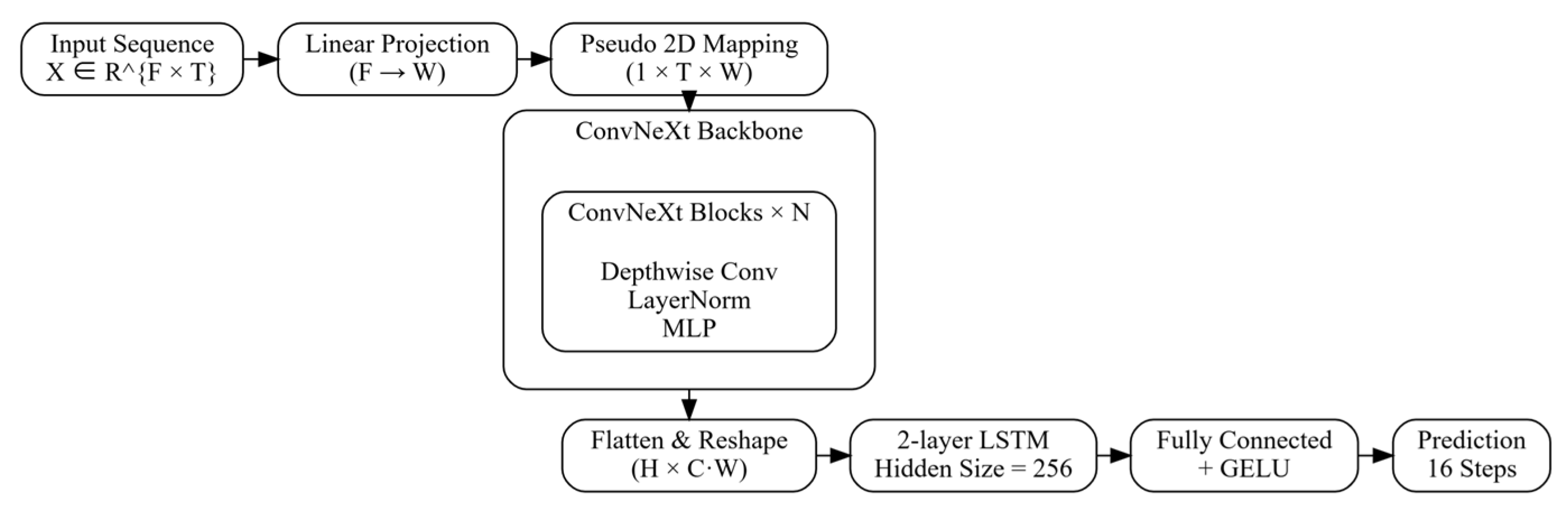
To investigate the applicability of two-dimensional spatial convolutions to time-series modeling, an ablation model is constructed in which the temporal CNN encoder is replaced with a ConvNeXt backbone. The procedure is as follows:

• The time series $\mathbf{X}\in {\mathbb{R}}^{F\times L}$ is projected into a pseudo-two-dimensional representation;
• ConvNeXt is applied to extract “temporal–feature image” representations;
• The spatial dimensions are flattened and subsequently fed into an LSTM module to model temporal evolution.

The overall structure is expressed as:

$$\mathbf{Z}=\mathrm{C}\mathrm{o}\mathrm{n}\mathrm{v}\mathrm{N}\mathrm{e}\mathrm{X}\mathrm{t}(\varphi (\mathbf{X})),h_t=\mathrm{L}\mathrm{S}\mathrm{T}\mathrm{M}(\mathbf{Z}),{\hat{\mathbf{Y}}}_t=f_{\mathrm{f}\mathrm{c}}\left(h_t\right).$$

(32)

This model is designed to examine whether the translation-invariant convolutional inductive bias that has proven successful in computer vision remains suitable for PV power time series characterized by strong periodicity and non-stationarity.

The overall pipeline of the ConvNeXt–LSTM ablation model is presented in Figure 1, which visualizes the data flow from pseudo-two-dimensional projection to spatial feature extraction with ConvNeXt, and finally to temporal modeling using LSTM.

3.4.2. Unified Training and Hyperparameter Settings

To ensure fair comparison, all models are trained under identical data splits, number of training epochs, optimizer type, initial learning rate, and batch size. The random seed is fixed to eliminate stochastic fluctuations during training. The main structural parameters are summarized in

Table 2. Main structural parameters of all models.

Model	Layers Depth	Hidden Dimension	Kernel/Heads
LSTM	2-layer LSTM	256	N/A
TCN	4 Residual Blocks (Causal)	128	K = 3, D = {1, 2, 4, 8}
Transformer	3-layer Encoder	128	4 Heads
CNN–LSTM	3 Conv1d + 2 LSTM layers	128 (CNN)/256 (LSTM)	K = {7, 5, 3}
ConvNeXt–LSTM	Atto-scale CNN + 2 LSTM layers	256 (LSTM)	7 × 7 (Large Kernel)

.

As shown in Table 2, the models differ in depth, hidden dimensions, and convolutional structures, resulting in variations in parameter scale. Because strict parameter matching is not enforced, the comparative results should be interpreted primarily as reflecting how different architectural designs perform under a unified experimental setting, rather than as a fully capacity-controlled comparison.

Although no clear monotonic relationship is observed between parameter count and forecasting error, the potential influence of model capacity cannot be excluded. Therefore, the robustness and ablation results presented in the following sections should be interpreted with caution, as part of the observed performance gains may be attributable to differences in model capacity rather than architectural suitability alone.

3.5. Multi-Model Multi-Step Forecasting Performance Comparison

The selected PV plant in Inner Mongolia is located in a region characterized by highly volatile meteorological conditions. This setting introduces significant challenges for forecasting, as multi-step prediction must remain robust under frequent weather-induced power fluctuations. The forecasting task involves a long input window (96 steps) and a 4 h (16-step) multi-step-ahead prediction. Compared with single-step forecasting, multi-step prediction suffers from error accumulation effects. Furthermore, the test set contains numerous cloudy and rainy samples, increasing modeling difficulty.

Therefore, this study focuses on the relative performance of different structural inductive biases rather than on pursuing the absolute minimum error under specific hyperparameter configurations.

Under a unified dataset (maximum power 12,503.37 kW; mean power 3165.66 kW), input window length (L = 96), and forecasting horizon (H = 16), four mainstream time-series models and the ablation model are quantitatively evaluated. MAE and RMSE are computed after inverse normalization to the actual plant-level power scale (kW), considering only daytime samples (power > 100 kW), to ensure that the evaluation is conducted in a physically meaningful operating range.

3.5.1. Quantitative Results

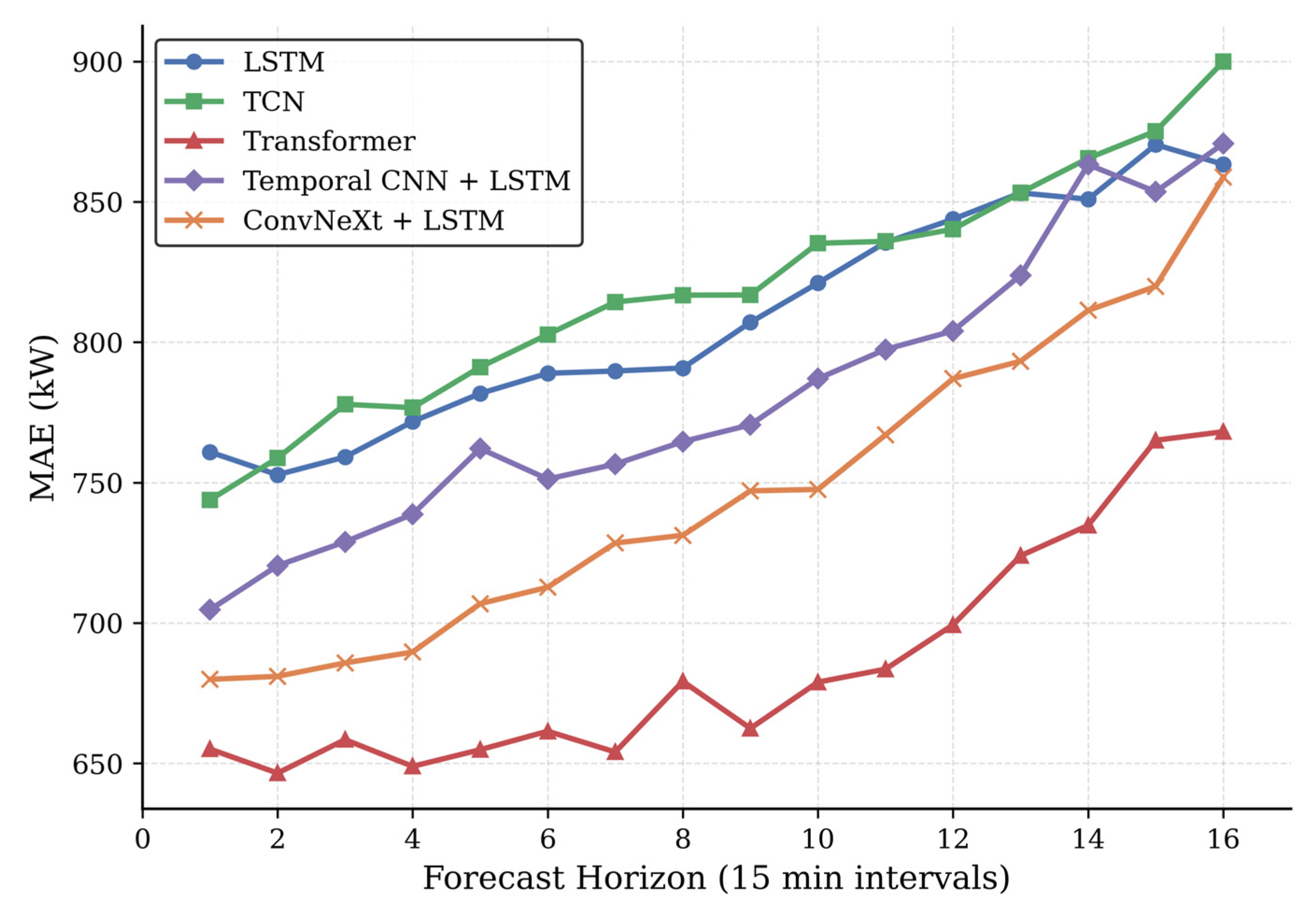
Figure 2 illustrates the evolution of step-wise MAE for all evaluated models over the 16-step (4 h) forecasting horizon.

Under the unified experimental setting, the multi-step forecasting errors on the validation set are listed in

Table 3. Validation-set performance of different models for 16-step ultra-short-term PV forecasting.

Model	Parameter	RMSE (kW)
LSTM	1440.26	2109.98
TCN	1443.70	2112.48
Transformer	1229.49	1814.07
CNN–LSTM	1407.78	2073.23
ConvNeXt–LSTM	1345.35	1988.34

.

Table 3 shows that the Transformer achieves the best overall accuracy under the current 16-step forecasting setting, with the lowest MAE and RMSE. ConvNeXt–LSTM ranks second and performs better than LSTM, TCN, and CNN–LSTM in the same experiment. Therefore, the relevance of ConvNeXt–LSTM in this study lies not in being the best overall forecasting model, but in providing a competitive hybrid alternative whose behavior remains relatively stable in the subsequent robustness analyses. Within the present single-site, fixed-horizon setting, these results indicate that introducing a vision-derived convolutional encoder can improve performance over conventional recurrent or temporal convolution baselines, while still remaining below the Transformer benchmark.

3.5.2. Ablation Study: Replacing Temporal CNN with ConvNeXt

To analyze the suitability of deep vision-based convolutional structures for time-series tasks, the temporal CNN encoder is replaced with a ConvNeXt backbone while keeping all other training settings unchanged.

The results show that under identical conditions:

$${ \mathrm{MAE} }_{\mathrm{ConvNeXt}+\mathrm{LSTM} }<{ \mathrm{MAE} }_{\mathrm{TemporalCNN}+\mathrm{LSTM} }.$$

(33)

MAE decreases from 1407.78 kW to 1345.35 kW; RMSE decreases from 2073.23 kW to 1988.34 kW. Both metrics exhibit consistent reductions.

This finding suggests that the large receptive field and grouped convolution design of ConvNeXt enable more comprehensive extraction of multi-scale features within intra-day power evolution.

However, it should be noted that ConvNeXt remains fundamentally based on the translation invariance assumption, whereas PV time series possess strong time-position semantics and non-stationary characteristics. Therefore, the performance improvement is more likely attributable to receptive field expansion and enhanced channel representation capacity, rather than to the intrinsic physical appropriateness of the convolutional inductive bias itself.

This phenomenon is further discussed in subsequent robustness and structural analyses.

3.5.3. Statistical Significance and Error Distribution Analysis

To validate the statistical reliability of performance differences among models, non-parametric significance tests are conducted on step-wise forecasting errors in the test set. Considering that error distributions may deviate from normality, the Wilcoxon signed-rank test is employed for paired MAE comparisons between models.

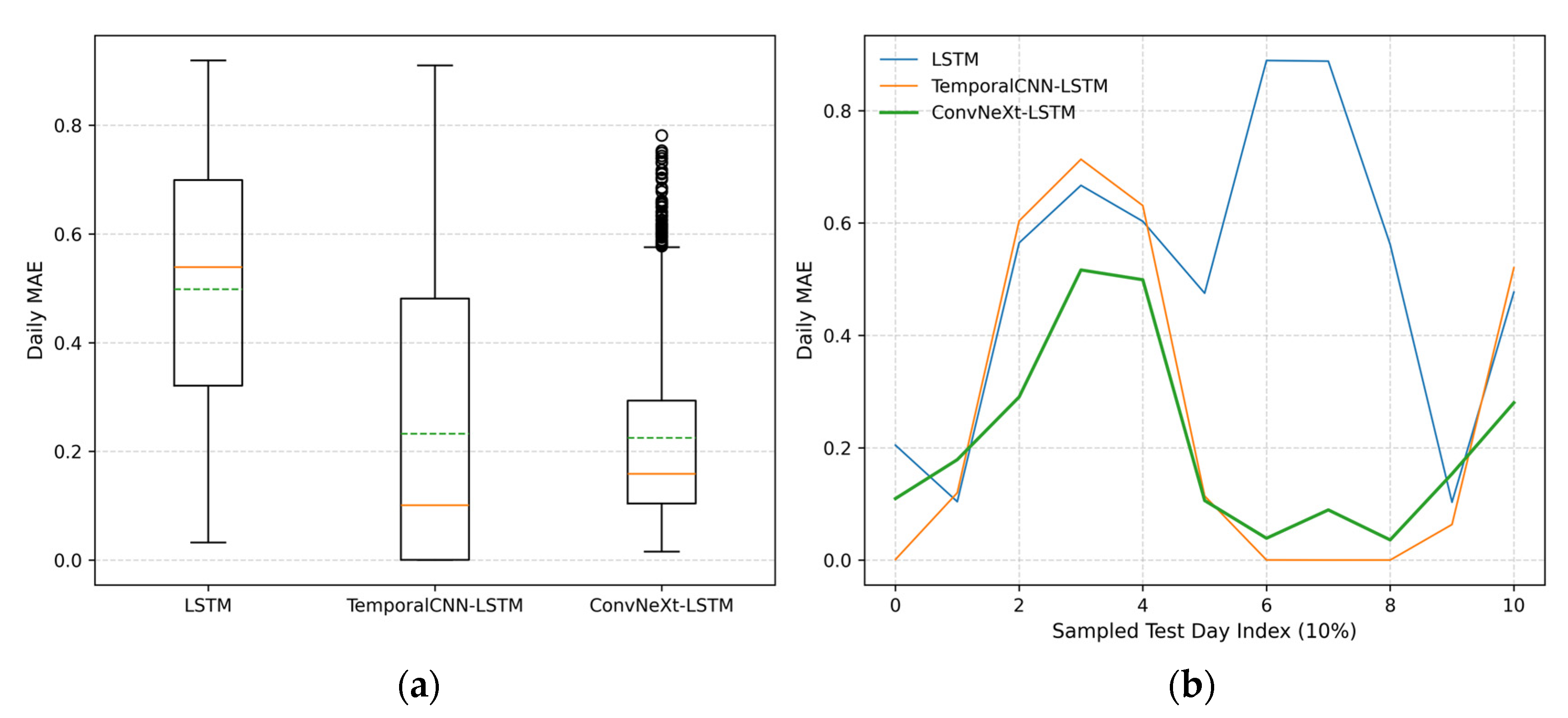
Figure 3 presents a comparative analysis of daily forecasting errors across the three models. Specifically, Figure 3a displays the distribution of daily MAE, where it is evident that the ConvNeXt–LSTM model (represented by the green distribution) exhibits a more concentrated error density in the lower range compared to the standard LSTM and CNN–LSTM models. This indicates superior stability in daily performance. Figure 3b illustrates the daily MAE variation over the test period. The temporal trend shows that while all models experience performance fluctuations due to varying weather conditions, the ConvNeXt–LSTM architecture consistently maintains lower error peaks, particularly during periods of high solar volatility. These results confirm that the integration of the ConvNeXt backbone effectively enhances the model’s robustness in capturing complex daily power patterns.

First, the prediction errors of ConvNeXt–LSTM and the conventional LSTM are compared. The results indicate that p < 0.001, demonstrating statistical significance at the 95% confidence level. This confirms that the error reduction achieved by introducing a deep convolutional encoder is not attributable to random fluctuations but reflects a stable statistical advantage.

Subsequently, ConvNeXt–LSTM is compared with CNN–LSTM. The test yields p = 0.7176, which exceeds 0.05, indicating that the difference does not reach statistical significance. This suggests that, under the current data scale and forecasting configuration, the two convolutional encoding structures exhibit statistically comparable performance.

These results indicate that deep convolutional encoders consistently outperform traditional recurrent structures. However, the performance differences among hybrid architectures (e.g., temporal CNN vs. ConvNeXt) remain relatively small, suggesting that increased structural complexity does not necessarily yield statistically significant improvements in forecasting accuracy.

Furthermore, analysis of the MAE distributions shows that ConvNeXt–LSTM exhibits a lower standard deviation (173.26 kW) than CNN–LSTM (270.17 kW), indicating reduced prediction variability and enhanced stability.

Overall, the statistical results strengthen the reliability of the experimental conclusions.

3.6. Robustness Analysis of Prediction Performance Under Different Loss Functions

Photovoltaic (PV) power time series exhibit significant non-stationarity and strong amplitude fluctuations. Different loss functions vary in their sensitivity to outliers, peak intervals, and low-power periods, which may substantially affect training stability and final prediction performance.

To examine the dependency of model conclusions on the choice of error metric, five mainstream regression loss functions were introduced under a unified network architecture and training strategy:

• Huber Loss (abbreviated as Huber)

$${\mathcal{L}}_{\mathrm{Huber} }=\left\{\begin{array}{ll}{\displaystyle \frac{1}{2}}(y-\hat{y}{)}^2,& |y-\hat{y}|\le \delta \\ \delta |y-\hat{y}|-{\displaystyle \frac{1}{2}}{\delta }^2.& \mathrm{otherwise} \end{array}\right.$$

(34)

2.

Mean Squared Error (abbreviated as MSE)

$${\mathcal{L}}_{\mathrm{M}\mathrm{S}\mathrm{E}}={\displaystyle \frac{1}{N}}{\displaystyle {\sum }_{i=1}^N} {\left(y_i-{\hat{y}}_i\right)}^2.$$

(35)

3.

Relative Smooth L1 Loss (abbreviated as RSL1)

$${\mathcal{L}}_{\mathrm{RelHuber} }=\mathrm{S}\mathrm{m}\mathrm{o}\mathrm{o}\mathrm{t}\mathrm{h}\mathrm{L}1\left({\displaystyle \frac{\hat{y}-y}{y+\epsilon }},0\right).$$

(36)

4.

Daytime Weighted Relative Error Loss (abbreviated as Weighted-Rel)

$${\mathcal{L}}_{\mathrm{Weighted} }={\displaystyle \frac{1}{N}}{\displaystyle {\sum }_{i=1}^N} w\left(y_i\right)\cdot \mathrm{S}\mathrm{m}\mathrm{o}\mathrm{o}\mathrm{t}\mathrm{h}\mathrm{L}1\left({\displaystyle \frac{{\hat{y}}_i-y_i}{y_i+\epsilon }},0\right).$$

(37)

Here, the weighting function $w$(·) increases with power magnitude to emphasize prediction accuracy during high-generation daytime periods.

5.

Mean Squared Logarithmic Error (abbreviated as MSLE)

$$L={\displaystyle \frac{1}{n}}{\displaystyle {\sum }_{i=1}^n} {\left(\mathrm{l}\mathrm{n}\left(y_i+ϵ+1\right)-\mathrm{l}\mathrm{n}\left({\hat{y}}_i+ϵ+1\right)\right)}^2.$$

(38)

Variable Definitions:

• L: computed loss value (Loss);
• n: number of samples (total elements in pred or target);
• ${\hat{y}}_i$: model prediction;
• $y_i$: ground-truth label;
• $ϵ$: hyperparameter eps to prevent numerical instability caused by ln(0) (default value 10⁻⁶);
• $ln$: natural logarithm;

Under the five loss functions above, Model D (CNN–LSTM) and the ablation model (ConvNeXt–LSTM) were trained separately. To reduce the impact of random initialization, experiments were repeated using three different random seeds (42, 2026, 123). Daytime MAE and RMSE were calculated on the same validation set after inverse normalization.

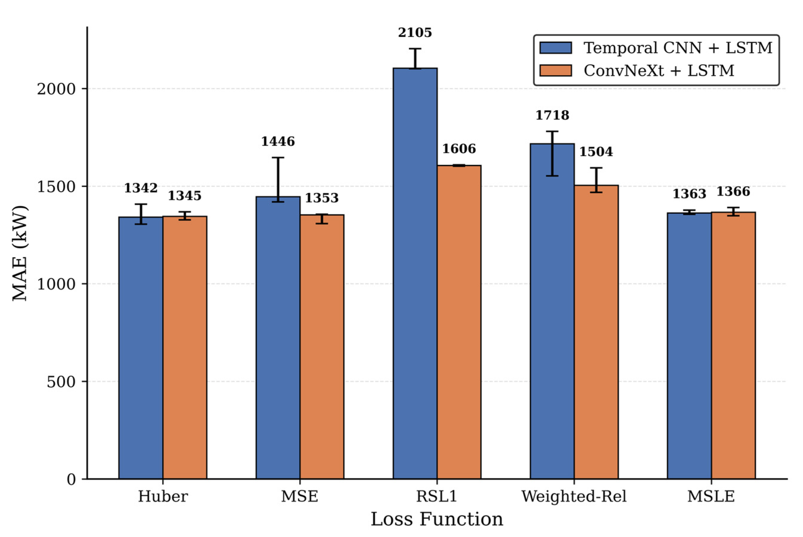
To evaluate the sensitivity of the models to different training objectives and initialization states, Figure 4 illustrates the median MAE performance and the corresponding min-max range across five distinct loss functions. By repeating experiments with three different random seeds (42, 2026, and 123), we observe that the ConvNeXt–LSTM model (the ablation model) consistently achieves lower median daytime MAE and RMSE values compared to the standard CNN–LSTM (Model D) under all tested loss functions. Furthermore, the narrower min-max range (indicated by the shaded areas) for the ConvNeXt–LSTM architecture suggests that the proposed model is more stable and less susceptible to the variations caused by random weight initialization. This comparative analysis demonstrates that the structural advantages of the ConvNeXt backbone are robust across different optimization criteria, reinforcing its suitability for reliable solar power forecasting.

To reduce the potential bias introduced by specific optimization objectives, the predictive performance under various loss function configurations is summarized in

Table 4. Performance comparison of different models for 16-step ultra-short-term PV forecasting.

Model	Loss	MAE (kW)	RMSE (kW)
CNN–LSTM	Huber	1351.56 ± 51.96	2023.53 ± 50.54
CNN–LSTM	MSE	1503.81 ± 124.64	2158.68 ± 61.16
CNN–LSTM	RSL1	2136.91 ± 58.10	2860.86 ± 84.49
CNN–LSTM	Weighted-Rel	1683.71 ± 117.51	2361.54 ± 151.27
CNN–LSTM	MSLE	1365.45 ± 11.01	1994.81 ± 24.03
ConvNeXt–LSTM	Huber	1346.93 ± 20.76	2002.96 ± 25.95
ConvNeXt–LSTM	MSE	1339.18 ± 26.68	1969.92 ± 46.72
ConvNeXt–LSTM	RSL1	1605.77 ± 3.53	2223.20 ± 50.15
ConvNeXt–LSTM	Weighted-Rel	1521.96 ± 64.67	2199.57 ± 73.10
ConvNeXt–LSTM	MSLE	1368.34 ± 20.82	1995.21 ± 19.44

. The experimental results show that ConvNeXt–LSTM maintains competitive forecasting accuracy across different settings, indicating that its performance ranking remains relatively stable under the studied loss designs. However, because strict parameter matching was not enforced, these results should be interpreted as evidence of comparative robustness within the present experimental setting, rather than definitive proof that the observed advantage arises solely from architectural superiority. Detailed results obtained using three random seeds (42, 123, and 2026) are provided in Appendix A (

Table A1. Detailed prediction errors under different loss functions (seed = 42).

Model	Loss	MAE (kW)	RMSE (kW)
CNN–LSTM	Huber	1407.78	2073.23
CNN–LSTM	MSE	1646.12	2228.71
CNN–LSTM	RSL1	2105.03	2846.28
CNN–LSTM	Weighted-Rel	1717.85	2442.11
CNN–LSTM	MSLE	1355.95	1987.09
ConvNeXt–LSTM	Huber	1345.35	1988.34
ConvNeXt–LSTM	MSE	1308.49	1920.96
ConvNeXt–LSTM	RSL1	1608.93	2275.54
ConvNeXt–LSTM	Weighted-Rel	1468.06	2142.74
ConvNeXt–LSTM	MSLE	1348.61	2006.70

,

Table A2. Detailed prediction errors under different loss functions (seed = 2026).

Model	Loss	MAE (kW)	RMSE (kW)
CNN–LSTM	Huber	1341.60	2025.16
CNN–LSTM	MSE	1446.50	2133.11
CNN–LSTM	RSL1	2203.93	2951.70
CNN–LSTM	Weighted-Rel	1552.94	2187.09
CNN–LSTM	MSLE	1377.53	1975.59
ConvNeXt–LSTM	Huber	1368.43	2032.92
ConvNeXt–LSTM	MSE	1352.93	1974.80
ConvNeXt–LSTM	RSL1	1606.41	2176.24
ConvNeXt–LSTM	Weighted-Rel	1593.68	2282.00
ConvNeXt–LSTM	MSLE	1390.10	2006.17

and

Table A3. Detailed prediction errors under different loss functions (seed = 123).

Model	Loss	MAE (kW)	RMSE (kW)
CNN–LSTM	Huber	1305.30	1972.19
CNN–LSTM	MSE	1418.81	2114.22
CNN–LSTM	RSL1	2101.78	2784.61
CNN–LSTM	Weighted-Rel	1780.35	2455.43
CNN–LSTM	MSLE	1362.87	2021.76
ConvNeXt–LSTM	Huber	1327.00	1987.63
ConvNeXt–LSTM	MSE	1356.12	2014.00
ConvNeXt–LSTM	RSL1	1601.96	2217.82
ConvNeXt–LSTM	Weighted-Rel	1504.15	2173.97
ConvNeXt–LSTM	MSLE	1366.32	1972.77

).

3.6.1. Overall Trends Across Loss Functions

Across three random seeds, ConvNeXt–LSTM consistently outperformed CNN–LSTM under Huber, MSE, and MSLE losses, with larger gains under MSE and Huber, indicating robust reproducibility beyond random initialization. While different loss functions altered error scale and sensitivity—MSE emphasizing outliers, MSLE reducing fluctuations, and RSL1 amplifying low-power errors—the overall model ranking remained unchanged. Notably, ConvNeXt–LSTM still achieved an approximately 24.8% MAE reduction under RSL1, demonstrating strong cross-loss robustness.

3.6.2. Sensitivity Analysis of Hybrid Models to Loss Function Selection

Overall, altering the loss function influences the scale of MAE and RMSE more substantially than it alters the relative performance ranking of the two hybrid models. ConvNeXt–LSTM remains competitive across the evaluated loss functions; however, the magnitude of its advantage varies depending on the optimization objective and should not be interpreted as uniformly large under all conditions. As parameter matching was not enforced, the findings in this section should be interpreted as evidence of comparative robustness within the current experimental setup, rather than conclusive proof that the observed differences stem solely from differences in model architecture. Detailed results for random seeds 42, 123, and 2026 are provided in Appendix A.

3.7. Temporal Adaptation and Receptive Field Sensitivity of ConvNeXt

This section focuses on three questions: whether larger receptive fields improve short-horizon PV forecasting, how much additional channel width helps under the current dataset, and whether deeper variants provide accuracy gains commensurate with their added complexity.

Using a controlled-variable approach, while keeping the LSTM structure, training epochs, optimizer, and Huber loss fixed, three structural dimensions were investigated:

• Kernel size $k$: to examine the ability of local receptive fields to capture PV power fluctuation patterns.

$$k\in \{3,5,7\}.$$

(39)

2.

Network depth d: modified through backbone variants (Atto and Nano) to evaluate the gain from deeper hierarchical feature abstraction.

3.

Channel width W: feature projection width (pseudo-image width), determining the representational capacity of spatiotemporal encoding.

$$W\in \{32,64,128\}.$$

(40)

All parameter combinations were systematically explored, and prediction errors under the optimal configurations were recorded.

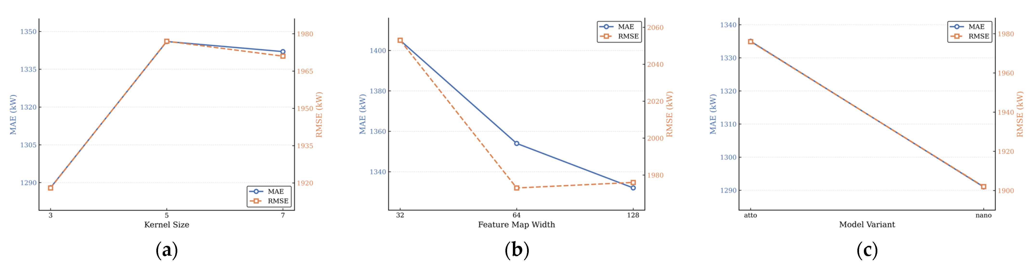
To systematically investigate the influence of structural parameters on the model performance, an extensive ablation study was conducted. Figure 5 presents the forecasting errors (MAE and RMSE) under different configurations. Specifically, Figure 5a examines the effect of various kernel sizes, while Figure 5b and Figure 5c illustrate the sensitivity of the model to channel width and architectural complexity, respectively.

To further quantify the trade-off between predictive accuracy and computational cost, the detailed numerical results and model parameters (M) for the ablation study are consolidated in

Table 5. Sensitivity analysis of ConvNeXt–LSTM performance and computational complexity across different structural hyperparameter configurations.

Dimension	Parameter	Setting	RMSE (kW)	MAE (kW)	Parameters (M)
Kernel Size (k)	Kernel Size	3	1917.97	1288.03	0.85
		5	1977.58	1345.91	0.92
		7	1972.65	1332.79	1.01
Channel Width (w)	Project Width	32	2052.96	1403.13	0.42
		64	1970.24	1353.96	0.76
		128	1972.65	1332.79	1.01
Network Depth (d)	Model Variant	Atto	1972.65	1332.79	1.01
		Nano	1905.04	1291.08	2.54

. While Figure 2 visualizes the error trends, Table 5 provides a precise record of MAE, RMSE, and the corresponding model scale for each configuration, facilitating a deeper analysis of structural efficiency.

3.7.1. Impact of Receptive Field Scale

From Table 5, under the current dataset and forecasting setup, the smallest kernel size (k = 3) achieved the lowest MAE (1288.03 kW), outperforming k = 5 and k = 7.

This indicates that in ultra-short-term forecasting tasks, small-scale convolution kernels (k = 3) are more effective at capturing abrupt short-term fluctuations in PV output. In contrast, larger kernels expand the receptive field but introduce a smoothing effect that may obscure high-frequency local variations, leading to slight performance degradation.

The relatively limited error differences among kernel sizes suggest diminishing marginal returns from receptive field expansion at this task scale.

3.7.2. Feature Width and Model Capacity

As the feature projection width increased from 32 to 128, the MAE exhibited a consistent decline, falling from 1403 kW to 1332 kW. This trend suggests that under a fixed network depth, expanding channel dimensions enhances the model’s capability to represent complex multivariate meteorological information. However, the performance gain is non-linear; specifically, the rate of error reduction diminishes as the width increases. This indicates the existence of a representation capacity saturation point for the specific PV dataset, where excessive channel expansion yields diminishing marginal gains in forecasting accuracy.

3.7.3. Network Depth and Hierarchical Feature Abstraction

The Nano variant (2.54 M parameters) achieved lower prediction error (1291 vs. 1332 kW) compared to the Atto variant (1.01 M parameters).

This demonstrates that increasing network depth facilitates higher-level abstract feature extraction.

However, although Nano achieved the lowest error, its parameter count is approximately 2.5 times that of Atto. From an engineering deployment and computational efficiency perspective, the marginal accuracy improvement may not justify the substantial increase in computational cost. Thus, a trade-off between complexity and accuracy remains necessary.

3.7.4. Structural Insights

The ablation results suggest that the benefit of ConvNeXt-style design in this task is conditional rather than monotonic. Smaller kernels are more suitable for capturing short-term local fluctuations, while wider and deeper backbones can reduce error but with diminishing returns and higher model cost. Taken together, the results indicate that performance depends on how well the structural design matches the temporal characteristics of the present forecasting task, not simply on increasing parameter count.

3.8. Feature Degradation Robustness Analysis

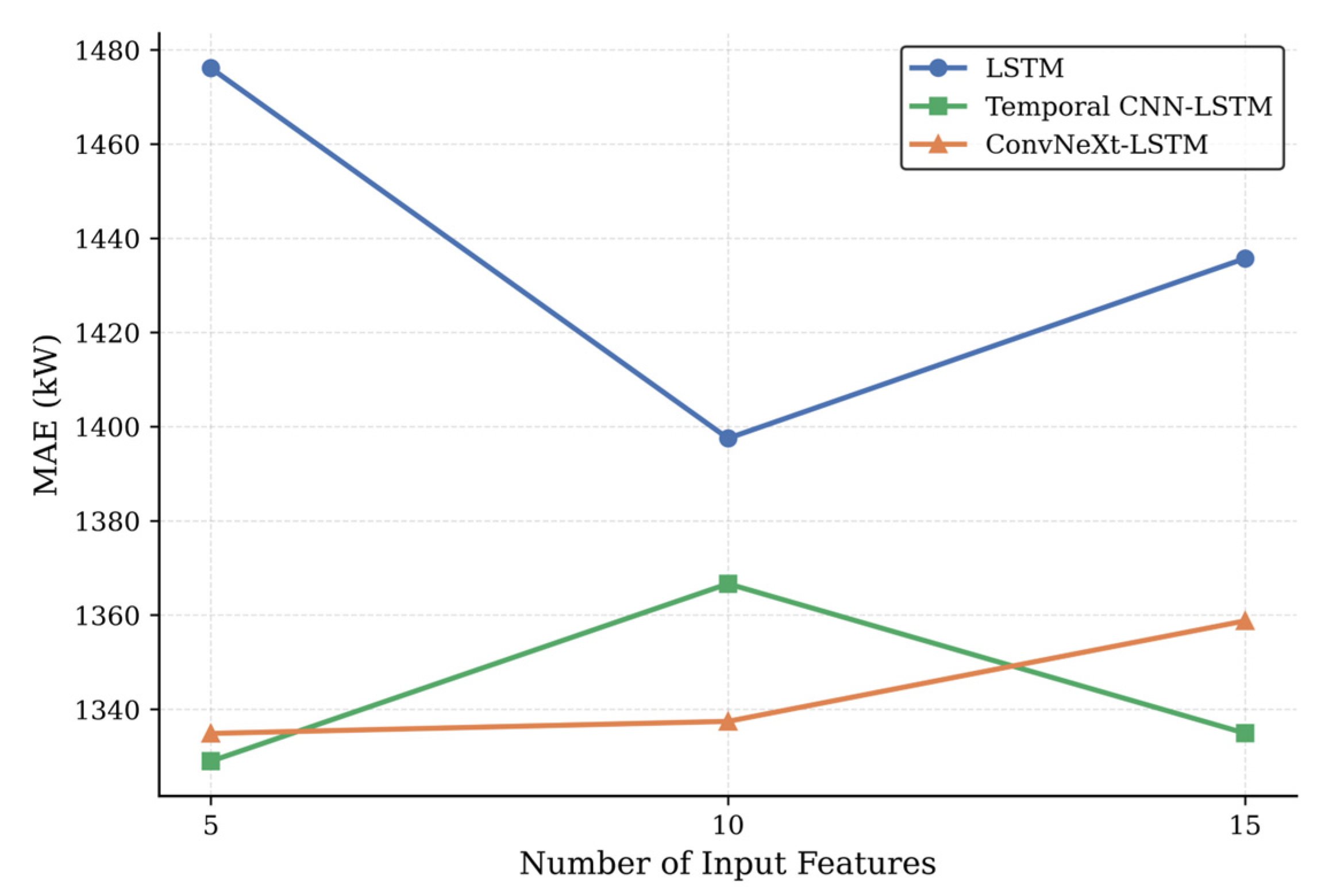
To evaluate model sensitivity to changes in input feature dimensionality, a feature degradation experiment was conducted. Three representative structures were evaluated under identical training strategies, preprocessing pipelines, and random seed settings: LSTM, CNN–LSTM, and ConvNeXt–LSTM.

As shown in Figure 6, the number of input features was progressively reduced from 15 to 10 and 5 to assess performance under limited information conditions. All experiments used Huber loss, and inverse-normalized daytime MAE was computed.

3.8.1. Performance Trends

The performance trends of the models under varying input feature dimensions exhibit distinct characteristics. The LSTM model displays noticeable fluctuations as the number of input features changes. Specifically, it achieves relatively better performance with 10 features, whereas higher errors occur in both the 15- and 5-dimensional settings. This behavior indicates that conventional recurrent architectures depend heavily on exogenous meteorological variables and possess limited ability to filter redundant information from high-dimensional inputs. Consequently, they are more susceptible to noise interference and exhibit performance deterioration when critical features are absent.

In contrast, the CNN–LSTM model performs strongly under the full-feature (15-dimensional) condition. However, its error increases markedly when the feature dimension is reduced to 10 and fluctuates further in the 5-dimensional setting. These results suggest that the model is sensitive to specific combinations of meteorological features and that its convolutional encoding process relies heavily on the availability and ordering of input variables.

The ConvNeXt–LSTM model, by comparison, maintains relatively stable MAE values as the feature dimension decreases from 15 to 5, showing substantially smaller fluctuations than the other two models. This stability underscores its superior robustness to feature degradation. The deep convolutional architecture enables effective extraction of spatiotemporal correlations even from limited input data, thereby compensating for the loss of exogenous features and supporting consistent predictive performance.

3.8.2. Structural Interpretation

PV power sequences exhibit clear periodicity and temporal semantic patterns (e.g., morning ramp-up, noon plateau, evening decay). If a model maintains stable prediction performance under reduced features, it implies stronger intrinsic temporal pattern modeling capability.

The stability of ConvNeXt–LSTM under feature degradation further supports the academic hypothesis of this study: in PV forecasting, the alignment between architectural inductive bias and intrinsic physical characteristics of time series contributes more to prediction accuracy than simple feature engineering stacking.

3.8.3. Feature Composition

The 15 selected features include:

• Time encoding features (hour_sin, hour_cos);
• Irradiation-related variables (IRRADIATION, surface_ssrd);
• Temperature and humidity variables (surface_skt, rh, surface_vpd);
• Wind field variables (surface_u10m, wd10m, etc.);
• Energy flux variables (sshf, slhf, str, etc.);

The 10-feature and 5-feature configurations were obtained through progressive feature elimination. The 5-feature set is a subset of the 10-feature set, and the 10-feature set is a subset of the 15-feature set.

The specific configurations of the reduced feature sets (F10 and F5) are summarized in

Table A4. Detailed description of input features and subset compositions.

Category	Feature Name	Variable Description	F15	F10	F5
Temporal Encoding	hour_sin	Sine component of the hour angle	●	●	●
	hour_cos	Cosine component of the hour angle	●	●	●
Solar Radiation	IRRADIATION	Ground-measured solar irradiance	●	●	●
	surface_ssrd	Surface solar radiation downwards	●	●	●
	str	Surface net thermal radiation	●	●
Atmospheric State	surface_tcc	Total cloud cover	●	●	●
	surface_skt	Skin temperature	●	●
	surface_vpd	Vapor pressure deficit	●	●
	rh	Relative humidity	●	●
Wind Field	surface_u10m	10 m u-component of wind	●	●
	wd10m	10 m wind direction	●
	surface_wd10m	Surface wind direction (10 m)	●
	surface_wd100m	Surface wind direction (100 m)	●
Energy Fluxes	sshf	Surface sensible heat flux	●
	slhf	Surface latent heat flux	●
Total Features			15	10	5

Note: ● indicates that the feature is included in the corresponding subset. The subsets follow a hierarchical structure: $F5\subset F10\subset F15$.

of Appendix B.

All models removed exactly the same features to ensure rigorous comparison. Time encoding and core irradiation variables were prioritized for retention.

4. Discussion

4.1. Conditional Performance Gains and Structural Boundaries of ConvNeXt-LSTM

Test set results show that ConvNeXt–LSTM exhibits more competitive performance under strict evaluation conditions compared with conclusions drawn from the validation set. Under specific loss functions and model configurations, its MAE and RMSE are lower than those of CNN–LSTM. These findings suggest that deep convolutional structures can effectively extract beneficial local variation patterns for photovoltaic power forecasting, particularly during daytime periods with intense power fluctuations.

However, this advantage is neither inherent to the model architecture nor universally guaranteed. Ablation experiments demonstrate that the predictive accuracy of ConvNeXt–LSTM is highly sensitive to convolution kernel size, channel width, and overall model scale. When the kernel size becomes excessively large or the channel width increases substantially, prediction error rises rather than declines. This indicates that simply enlarging the receptive field or increasing the parameter count does not continuously improve performance in time-series forecasting. The results highlight a clear diminishing marginal return when applying visual convolutional architectures to temporal prediction tasks.

4.2. Temporal Structural Mismatch and the Impact of Convolutional Inductive Bias

From a modeling perspective, the depthwise separable convolution and Layer Normalization adopted in ConvNeXt are fundamentally based on the translation invariance assumption of two-dimensional spatial convolution. While this assumption is highly effective in image tasks, it does not naturally align with photovoltaic time series, where different temporal positions (e.g., morning ramp-up, noon plateau, evening decay) correspond to distinct physical processes and statistical distributions.

In contrast, one-dimensional temporal convolution structures such as temporal CNN and TCN preserve temporal order and positional semantics more effectively through causal constraints and directional receptive field expansion. As a result, they exhibit more stable error degradation under longer forecasting horizons. This observation is consistent with the experimental results showing step-wise error growth in multi-step forecasting, providing additional evidence of temporal structural mismatch.

4.3. Loss Function Robustness and Stability of Conclusions

Across multiple loss function settings, the overall ranking of model performance remains consistent, indicating that the study’s conclusions are not dominated by the choice of a specific loss function.

Relative-error-based losses and weighted relative Huber losses demonstrate improved stability during high-power daytime intervals, effectively mitigating systematic peak-period bias. However, they do not alter the relative superiority among different model structures.

This further confirms that architectural design and temporal modeling mechanisms remain the primary determinants of forecasting performance [32].

4.4. Feature Degradation Robustness

An important observation from the feature ablation study is that increasing the number of input features does not necessarily yield monotonic improvements in forecasting accuracy. This finding suggests that photovoltaic power forecasting is predominantly governed by the inherent variability and uncertainty of solar generation, rather than by model capacity or feature richness alone [33].

Compared with conventional LSTM-based models, ConvNeXt–LSTM demonstrates superior robustness under reduced-feature conditions. This robustness can be attributed to the convolutional inductive bias introduced by the ConvNeXt backbone, which facilitates effective temporal aggregation and local pattern extraction prior to sequence modeling. Consequently, the model depends less on individual meteorological variables and is better suited to scenarios involving incomplete or noisy sensor data.

Furthermore, the consistent performance gains achieved with the Huber loss function indicate that robust loss formulations are more suitable for photovoltaic power forecasting tasks, in which occasional extreme errors may arise from sudden weather changes or measurement noise.

Overall, these results suggest that architectural robustness plays a significant role under feature-limited conditions in photovoltaic power forecasting. Nevertheless, because this study did not include a controlled comparison of training cost, inference latency, or deployment complexity across models, the current findings should not be interpreted as evidence of deployment superiority.

5. Conclusions and Future Work

5.1. Conclusions

This study proposed a hybrid modeling framework that integrates the visual convolutional backbone ConvNeXt with LSTM for ultra-short-term photovoltaic (PV) power forecasting. The model performs 16-step-ahead predictions (4 h ahead) at 15 min temporal resolution. Within a unified experimental setup, we conducted benchmark comparisons, structural ablation studies, statistical significance tests, and multidimensional robustness analyses. The main findings are summarized as follows:

First, the ConvNeXt–LSTM model significantly outperformed the conventional LSTM baseline in multi-step forecasting. Under the 16-step prediction horizon, MAE and RMSE decreased by approximately 6.6% and 5.8%, respectively. The Wilcoxon signed-rank test (p < 0.05) confirmed that these improvements were statistically significant, indicating that deep convolutional feature encoding effectively captures locally non-stationary temporal patterns in PV power time series.

Second, compared with the CNN–LSTM model, ConvNeXt–LSTM exhibited numerical improvements in forecasting accuracy; however, statistical tests showed that these differences were not significant. This result suggests that, at the current forecasting scale, ConvNeXt represents an optimized evolution of temporal convolutional architectures rather than a disruptive innovation. Its performance gains appear to be conditioned on specific structural characteristics.

Third, cross-loss experiments using MSE, Huber, MSLE, and weighted relative error demonstrated consistent performance rankings across models. Although robust loss functions such as Huber provided better convergence stability in high-power intervals, the architectural inductive bias remained the dominant factor influencing forecasting accuracy, rather than the choice of loss function.

Fourth, hyperparameter grid search results indicated that forecasting accuracy is not linearly correlated with receptive field size or channel width. Moderate structural expansion reduced prediction error, whereas excessive model scaling resulted in diminishing returns and, in some cases, performance degradation. These findings highlight that structural adaptation to the physical characteristics of PV time series is more critical than simple parameter scaling under the present task setting. However, because strict parameter matching was not performed, the isolated contribution of model capacity cannot be entirely ruled out.

Fifth, feature degradation experiments revealed that ConvNeXt–LSTM maintained strong performance resilience when the number of input features was reduced from 15 to 5 dimensions. Its sensitivity to feature completeness was markedly lower than that of the traditional LSTM model. This robustness arises from the convolutional encoding stage, which enables spatial aggregation and feature reconstruction across multivariate inputs, thereby improving practical applicability under sensor failures or missing data conditions.

In summary, this study demonstrates the effectiveness of integrating the ConvNeXt backbone into an LSTM-based framework for ultra-short-term multi-step PV power forecasting (15 min resolution, 16-step horizon) at a single PV plant. The ConvNeXt–LSTM model preserves the physical continuity of recurrent modeling while incorporating visual-domain inductive bias, achieving a favorable balance between prediction accuracy and computational robustness. Nevertheless, the findings are specific to the experimental conditions examined. Further validation across diverse datasets and operating conditions is required to assess the broader applicability of the proposed framework.

5.2. Future Work

Although this study employed a systematic experimental framework, several limitations remain.

First, the findings are based on a single PV power station dataset collected from one climate zone and a fixed forecasting task (15 min resolution, 4 h horizon). This restricts the generalizability of the proposed ConvNeXt–LSTM model. Future research should therefore evaluate its performance across multiple benchmark datasets that encompass diverse geographical locations, climate conditions, and seasonal variations to establish broader applicability.

Second, although non-parametric statistical significance testing was conducted, the robustness of the results could be further strengthened through repeated experiments and multiple random data splits.

Third, visual convolutional architectures inherently introduce a temporal semantic mismatch when applied to time-series forecasting tasks. Future studies could investigate explicit temporal positional encoding or lightweight attention mechanisms to better align convolutional inductive bias with the non-stationary dynamics of PV power time series.

Finally, from a practical deployment perspective, this work lacks a unified quantitative comparison of training cost, inference latency, and deployment complexity across models. Such controlled evaluations are essential before claiming practical superiority for real-time dispatching and embedded energy management applications.