


Abstract
To address the issue of inaccurate load forecasting affecting the effectiveness of minimum demand scheduling in railway traction stations, this study introduces a multi-objective grey wolf optimizer (MOGWO) to jointly optimize the parameters of variational mode decomposition (VMD) and long short-term memory network (LSTM) within the forecasting framework. The proposed MOGWO-VMD-LSTM model enhances the data decomposition capability of VMD and improves LSTM training, prediction accuracy, and inverse normalization reconstruction. Using a 10-day load dataset from a traction station, the model’s performance is compared against LSTM and VMD-LSTM baselines. Simulation results demonstrate superior performance in terms of mean absolute error (MAE), root mean squared error (RMSE), and mean absolute percentage error (MAPE) metrics. Application of the forecasting results to traction station scheduling reduces the single-peak power purchase from 22.279 MW to 20.052 MW, achieving a 9.995% reduction, indicating strong practical potential.
1. Introduction
With the development of modern railway systems, the minimum demand control method of traction substations has become a key technology to ensure both economic efficiency and stable operation of the power system [1,2]. Among the influencing factors, inaccurate load forecasting is the dominant issue that hinders the optimization of minimum demand scheduling strategies. To address this challenge, this paper proposes a load forecasting algorithm framework based on the multi-objective grey wolf optimizer (MOGWO) for jointly optimizing the parameters of variational mode decomposition (VMD) and long short-term memory (LSTM) networks, aiming to enhance forecasting accuracy.
In traditional load forecasting, signal decomposition techniques are typically applied to preprocess raw load data [3]. The data are decomposed into multiple physically meaningful intrinsic mode functions (IMFs), and separate prediction models are built for each mode, followed by reconstruction to obtain the final forecast [4]. To further improve prediction accuracy, researchers have focused on optimizing both the sequence preprocessing methods and the model parameters during reconstruction.
Hu et al. [5] introduced the sparrow search algorithm (SSA) to optimize VMD parameters and selected optimal feature subsets using the minimum redundancy maximum relevance (mRMR) method, combined with LSTM for prediction. In [6], the whale optimization algorithm (WOA) was used to determine VMD parameters and reconstruct the prediction model via a dual-mode economic mechanism. Luo et al. [7] also adopted a VMD+LSTM model and optimized LSTM hyperparameters such as the number of units, training epochs, and learning rate using an improved osprey algorithm.
Xiao et al. [8] improved the arithmetic optimization algorithm to find the best VMD decomposition parameters. In [9], a two-level optimization framework was proposed: SSA optimized the VMD parameters at the first level, while the improved salp swarm algorithm optimized LSTM parameters at the second level. The decomposed modal components were input into the second-stage model and superimposed for final predictions. Reference [10] combined WOA to optimize VMD’s decomposition parameters and used SSA to fine-tune LSTM parameters.
Although these methods improve the prediction accuracy of VMD-LSTM models and are of great practical value [11], the coupling relationship between preprocessing and prediction parameters still requires further investigation. Therefore, this paper proposes a VMD-LSTM collaborative optimization framework that simultaneously tunes VMD parameters (K and α) and LSTM parameters (hidden units and learning rate), balancing both prediction accuracy and decomposition quality. Because the VMD parameters and LSTM hyperparameters are interdependent, and adjusting one set directly affects the performance of the other. Simply combining all objectives into a weighted single objective cannot capture these coupled effects or guarantee balanced solutions. By treating the VMD-LSTM parameter set as a unified decision space and optimizing multiple targets simultaneously, the algorithm can search for parameter combinations that achieve a better trade-off. Due to MOGWO’s strong global search capability, fast and stable convergence, and its ability to naturally handle multiple conflicting objectives such as prediction accuracy and decomposition quality, it is simpler, more robust, and more effective at finding balanced parameter combinations suitable for complex nonlinear models compared to algorithms like particle swarm optimization (PSO), genetic algorithm (GA), or non-dominated sorting genetic algorithm II (NSGA-II). Therefore, the MOGWO algorithm is employed to optimize three objectives: maximize forecasting accuracy, minimize modal reconstruction error, and constrain model complexity. This approach prevents overfitting and information loss caused by imbalanced parameters. Based on this forecasting model, a minimum demand control strategy for traction substations is developed.
2. Parameter Coupling Between VMD and LSTM
The number of modes K and the penalty factor α in VMD mainly affect signal decomposition [12], while the number of hidden layer units and the learning rate in LSTM mainly affect prediction errors [13]. When performing collaborative multi-objective optimization, it is necessary to pay attention to the coupling relationship between these two types of parameters.
2.1. Effect of the Number of VMD Modes on LSTM Input Dimensions
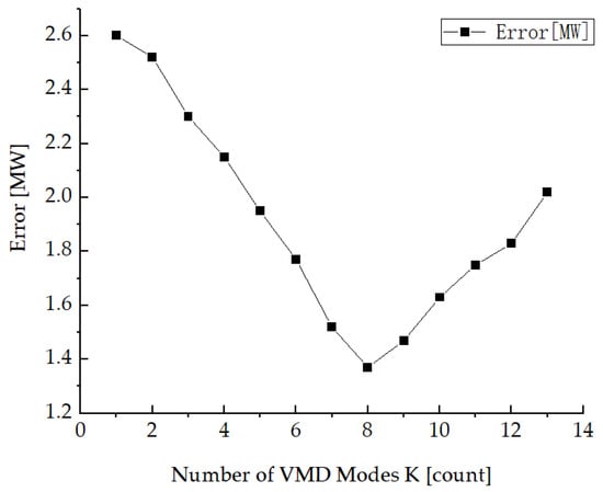
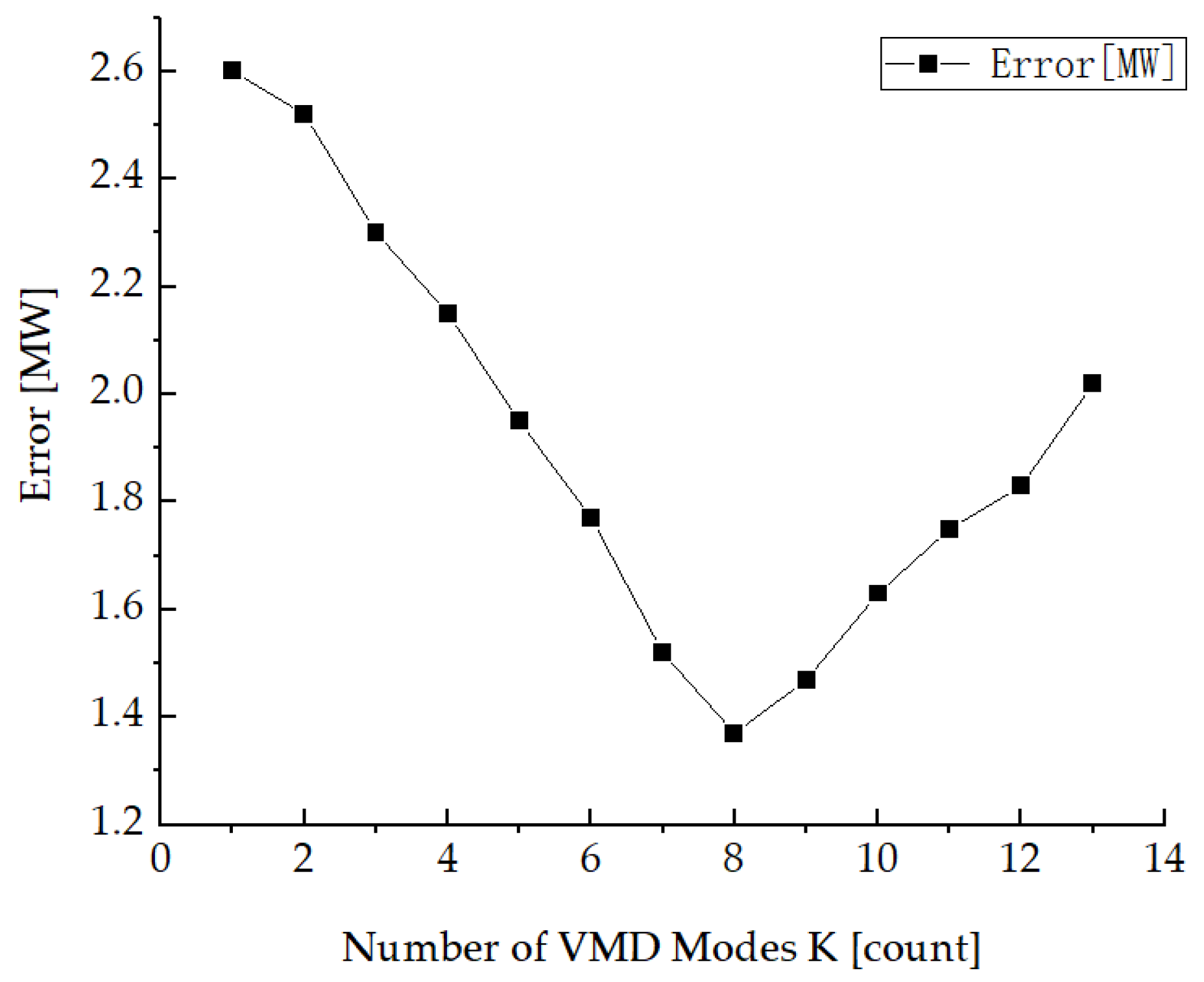
K determines the number of modes after decomposition [14], affecting the input feature dimension of the LSTM and directly influencing the model error. Fix the α and LSTM hyperparameters of VMD, only adjust the number of VMD modes K (1–13), repeat decomposition and training prediction, draw a curve based on the average error on the validation set to isolate the impact of K, ensuring that the error ‘first decreases and then increases’ is caused by changes in K. The relationship between the number of VMD modes K and the prediction error is shown in Figure 1.
Figure 1.
Relationship between VMD modal number K and prediction error.
A too-small K results in insufficient decomposition, noise residue, and information loss; the input feature dimension is low and of poor quality, causing higher errors. Increasing K expands the input feature dimension, helping the model capture patterns and reduce errors. However, if K exceeds a threshold, the input feature dimension becomes too high, leading to LSTM overfitting, reduced generalization ability, and a rise in errors.
2.2. Correlation Between VMD Penalty Factor and LSTM Temporal Modeling Capability
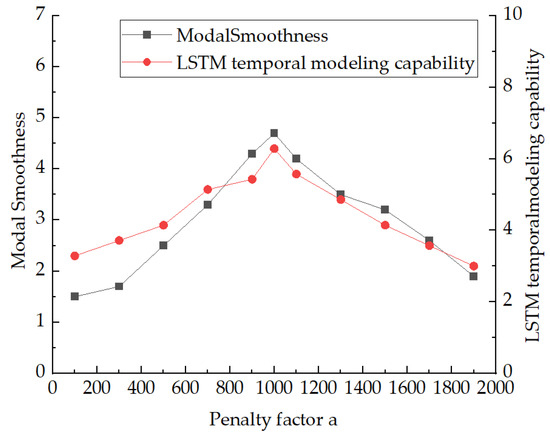
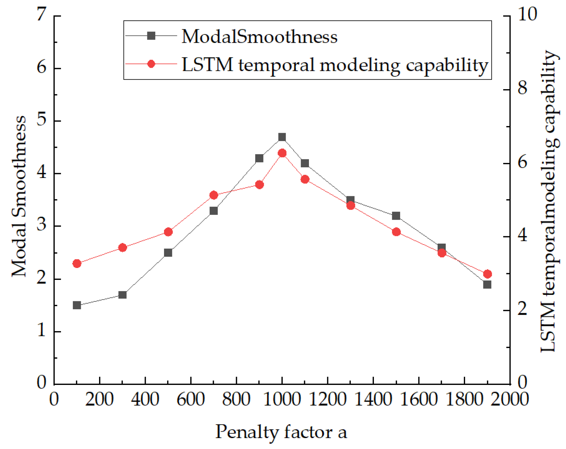
The penalty factor α of VMD indirectly affects the sequential modeling ability of LSTM by adjusting the smoothness and frequency distribution of the sub-signals [15]. With the VMD mode number K and LSTM hyperparameters fixed, only adjust the VMD penalty factor α (0–2000), repeatedly perform VMD decomposition and LSTM training, quantify and compare the modal smoothness and LSTM sequence modeling ability under different α values, isolating the effect of α to ensure that the variation trends in both are caused by changes in α. The impact of the penalty factor α on LSTM’s sequential modeling ability is shown in Figure 2.
Figure 2.
Effect of VMD penalty factor α on LSTM timing modeling ability.
α controls the bandwidth and smoothness of the VMD modes, influencing the modeling performance of LSTM. If α is too small, the mode bandwidth is wide and the smoothness is low [16], which is not conducive to LSTM feature extraction; moderately increasing α can narrow the bandwidth and improve smoothness, which benefits modeling; if α is too large, the modes become overly smooth, leading to loss of key information and reduced prediction accuracy. Here, both the VMD mode smoothness and the LSTM sequential modeling ability are dimensionless indices.
2.3. Synergistic Relationship Between the Number of LSTM Hidden Units and the Number of VMD Modes
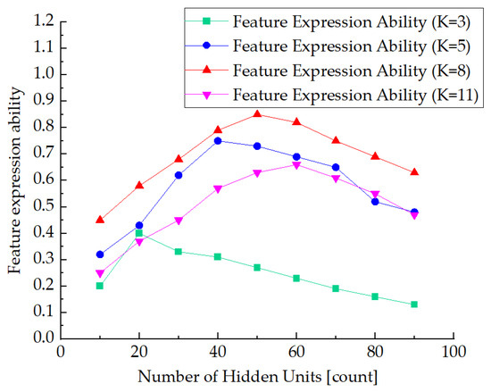
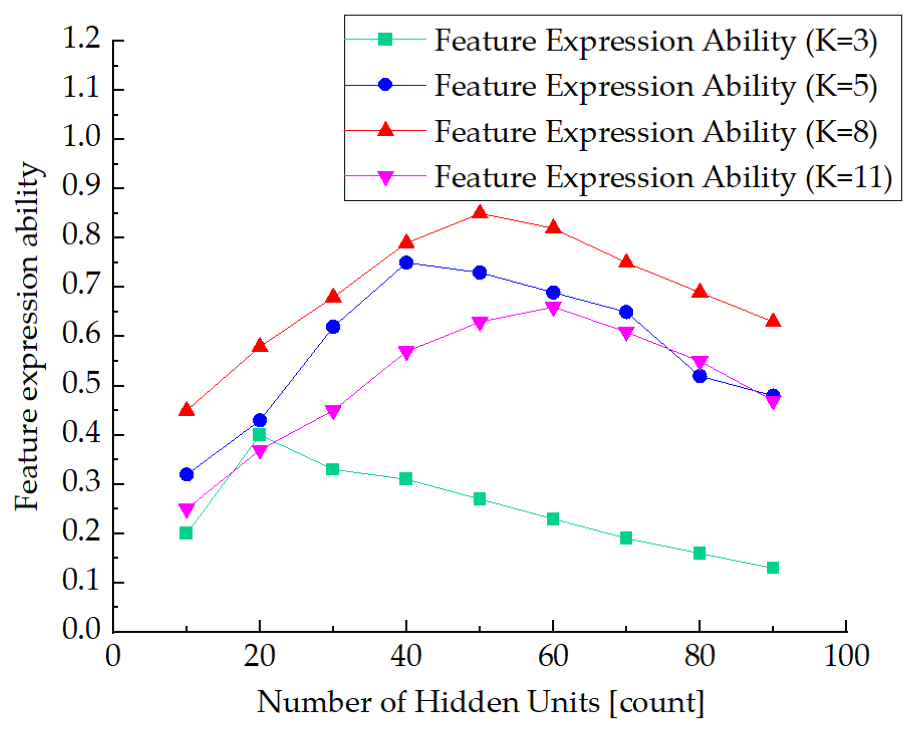
The number of LSTM hidden units directly determines the model capacity [17], and together with the VMD mode number K, it influences the model’s ability to represent multimodal features. Fix the VMD penalty factor α, only adjust the number of VMD modes K (3, 5, 8, 11) and the number of LSTM hidden units (0–100), repeat VMD decomposition and LSTM training, quantify the feature representation capability under different combinations, isolate the effects of K and the number of hidden units, and ensure that changes in feature representation capability are caused by the adjustments of these two parameters. The effects of the number of LSTM hidden units and the VMD mode number K on feature representation ability are shown in Figure 3.
Figure 3.
Effect of LSTM hidden cell number and VMD modal number K on feature expressiveness.
By adjusting the number of hidden units and K, the feature representation ability (dimensionless) first increases and then decreases. If K is too small, the modal complexity is low, and too many hidden units lead to redundant model capacity, amplifying data noise interference; if K is too large, the input modal features are rich, and too few hidden units make it difficult to capture complex nonlinear relationships among multimodal data, resulting in the loss of high-frequency modal features.
2.4. Overview of Parameter Co-Optimization Strategy
The parameters of VMD and LSTM are interdependent, and optimizing them in isolation can easily lead to parameter mismatch and performance degradation. Therefore, it is necessary to optimize both types of parameters collaboratively as a whole to determine the optimal parameter combination, ensuring efficient coordination between signal decomposition and predictive modeling.
3. A Load Forecasting Model Based on MOGWO for Cooperative Optimization of VMD–LSTM Parameters
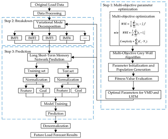
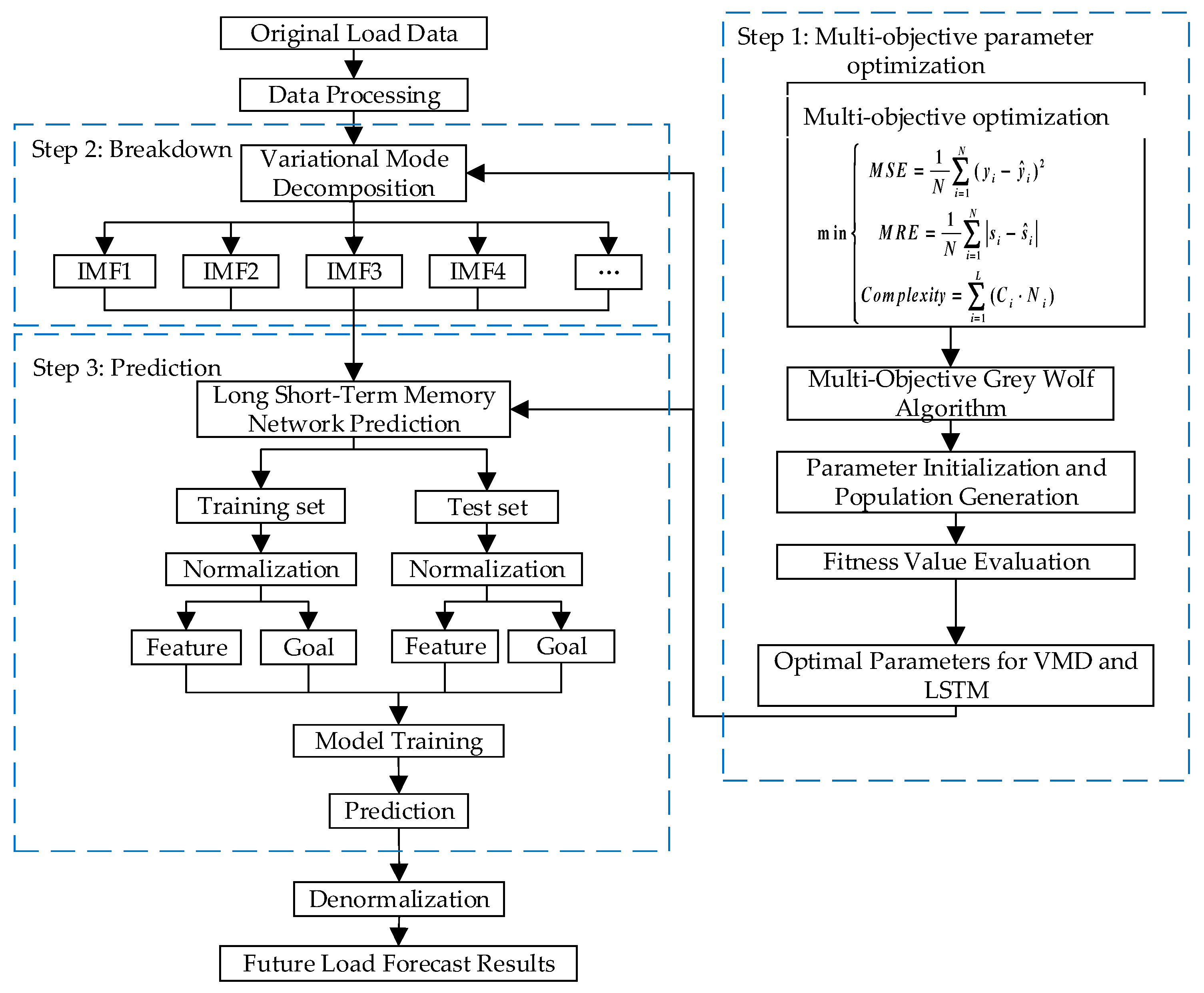
The MOGWO-VMD-LSTM prediction model is shown in Figure 4.
Figure 4.
MOGWO-VMD-LSTM flowchart.
In the algorithm, MOGWO optimizes by maximizing prediction accuracy, minimizing modal reconstruction error, and limiting network complexity. VMD decomposition parameters and LSTM network parameters are encoded into a unified solution vector and optimized simultaneously. This ensures that VMD produces high-quality feature sequences while constraining the complexity of the LSTM network to avoid overfitting. The code snippet is shown in Table 1.
Table 1.
Code snippet for joint parameter optimization of VMD–LSTM based on MOGWO.
In this study, the dataset was divided into training and testing sets using a time-based split. Specifically, the first 80% of the chronological data was used for model training, while the remaining 20% was reserved for testing. This strategy prevents future information leakage and is consistent with practical short-term load forecasting applications.
The specific steps for collaborative load forecasting using MOGWO-based VMD-LSTM are as follows:
- Step 1: The MOGWO algorithm obtains the optimal parameters for VMD and LSTM through multi-objective collaborative optimization.
- Step 2: The optimal parameters are input into the VMD model to decompose historical load data.
- Step 3: Each IMF component is input into the LSTM network for processing, followed by inverse normalization to obtain the final future load forecast results.
3.1. Parameter Synergy Optimization Strategy
MOGWO draws on the social hierarchy of gray wolf packs, dividing individuals into four main ranks: alpha, beta, delta, and omega wolves [18].
3.1.1. Predation Behavior Simulation
In VMD and LSTM parameter optimization, the ‘prey’ represents the position of the parameter combination that optimizes multiple objective functions, and the position can be updated using formulas as follows:
where refers to the position vector of the VMD and LSTM parameter combination in the t-th generation; is the position vector of the t-th generation prey (optimal solution); and are coefficient vectors, , , is the convergence factor, which decreases linearly with the number of iterations, , t is the current iteration number, T is the maximum number of iterations, and are random vectors uniformly distributed in the [0, 1] interval.
The process of α, β, and δ wolves leading omega wolves to hunt prey corresponds to guiding other parameter combinations toward better solutions. The specific formula is as follows:
where , , are the position difference vectors between the current individual and the three-tiered alpha wolf; , , represent the position vectors of the VMD and LSTM parameter combinations corresponding to the α, β, and δ wolves in the t-th generation. The final position of the ω wolf is obtained by averaging the three intermediate solutions, thereby achieving iterative optimization of the parameter combinations under multi-objective guidance, gradually approaching the global optimal parameter configuration.
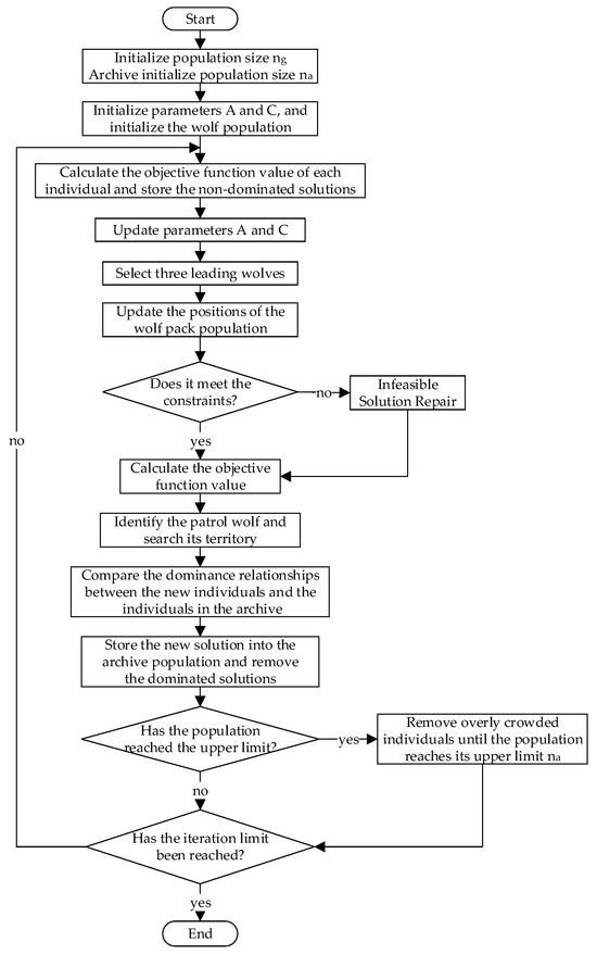
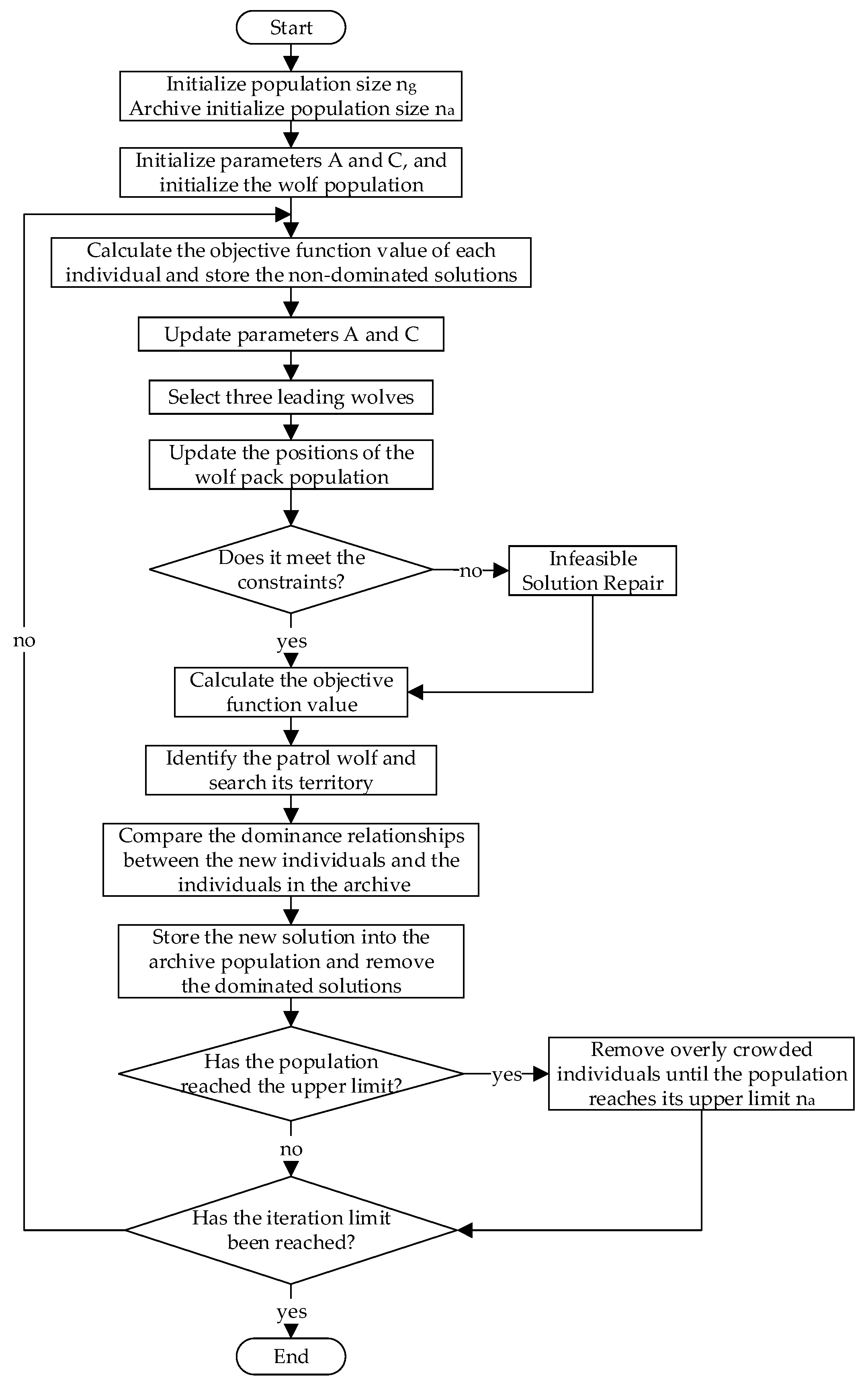
The specific implementation process of MOGWO is shown in Figure 5.
Figure 5.
MOGWO flowchart.
3.1.2. Crowd Distance Calculation
During the optimization process, the combination of parameters behaves differently across multiple objective functions. To ensure the diversity of parameter combinations, it is necessary to calculate the crowding distance, which is expressed as:
where, and are the function values at the i-th and i−1-th time steps in dimension j, respectively; and are the maximum and minimum values of the function f in dimension j. The total crowding distance of individual i di is the sum of the crowding distances of all objective functions. When selecting parameter combinations, individuals with larger crowding distances are given priority.
3.1.3. Multi-Objective Fitness Evaluation
When performing multi-objective optimization of VMD and LSTM parameters, each parameter combination corresponds to multiple objective function values:
- (1)
- Maximizing prediction accuracy
Minimizing the mean squared error (MSE) measures the predictive accuracy of a combination of parameters, and its expression is
where is the actual value of the i-th sample; is the predicted value of the i-th sample; N is the number of samples.
- (2)
- Modal reconstruction error minimization
Modal reconstruction error (MRE) mainly characterizes the accuracy of VMD signal decomposition, and its expression is
where si is the original signal of the i-th sample; is the reconstructed signal of the i-th sample; N is the total number of samples.
- (3)
- Network complexity minimization
To avoid prolonged training and excessive resource consumption from over-complex networks, we define the complexity of our LSTM-based model by first formalizing the parameter count of the i-th layer:
where Din,t is the i-th layer’s input dimension; Ni is the number of LSTM hidden units (nodes) in layer i; 4 is LSTM’s four gates; is the weight parameter of each gate; the final Ni represents bias terms.
The network complexity (total parameters) is
where L is the total number of layers.
Network complexity upper limit is defined as the minimum value of the total number of trainable parameters of the LSTM network. For multi-combination scenarios of network structure parameters, network complexity optimization uses a multi-objective constrained efficient search strategy. it balances the priority of prediction accuracy and parameter count through weighting coefficients, sets maximum parameter constraints to control resource consumption, and, with the help of Bayesian optimization’s probabilistic modeling and expected improvement criterion, can quickly find the optimal configuration that balances accuracy and complexity without the need for brute-force search.
3.1.4. Multi-Objective Grey Wolf Optimizer (MOGWO) Configuration and Final Solution Selection
To clarity of the optimization framework, this subsection presents the detailed configuration of the MOGWO. MOGWO is used to explore the coupled parameter space and generate a Pareto-optimal set of solutions, which reflects various trade-offs among accuracy, decomposition quality, and model complexity.
Table 2 summarizes the key configuration settings of the MOGWO. The listed hyperparameters—including population size, maximum iterations, number of objectives, and the α–β–δ leadership update strategy—define the search behavior and convergence characteristics of the optimizer. An adaptive external archive is used to store non-dominated solutions throughout the iterative process, ensuring that the entire Pareto front is effectively preserved without imposing rigid size constraints.
Table 2.
MOGWO Hyperparameters and Final Solution Selection Strategy.
In addition, the table specifies the criterion used to select the final solution from the generated Pareto front. Because MOGWO produces multiple trade-off solutions rather than a single optimum, the knee-point method is applied to identify the solution with the best balance among prediction accuracy, decomposition quality, and model complexity. This strategy ensures that the final VMD-LSTM parameter configuration achieves high forecasting performance without unnecessarily increasing model size.
3.2. Decomposition of Historical Load Data Using Optimal Parameter VMD
To effectively extract data features and improve the accuracy and efficiency of data processing, VMD is used for adaptive decomposition of the data. By constructing a variational optimization problem to recursively extract finite-bandwidth modal components [19], the original load signal is decomposed into K intrinsic mode functions, each having a specific central frequency, expressed as:
where is the reciprocal of time; is the Dirac function; j is the imaginary unit; * denotes the convolution operation; is the transformation of the frequency modulation of the signal.
Introducing the Lagrange multiplier λ(t) and the bandwidth parameter α, an augmented Lagrangian function is constructed to achieve constrained optimization. The Alternating Direction Method of Multipliers (ADMM) is used to iteratively update uk(t) and until the convergence threshold ε = 10−7 is met, at which point the iteration stops. The function is:
Lagrange multiplier λ(t) used to introduce signal reconstruction constraints is not a preset fixed value, but a variable that is automatically updated during the alternating direction method of multipliers (ADMM) iteration process.
Specifically, in each iteration, it is updated according to the following formula:
where n is number of iterations; τ is step size parameter; f(t) is original signal; is the sum of all modes at the current iteration.
3.3. Parallel LSTM Simulation for IMF Component Load Forecasting
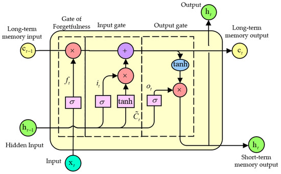
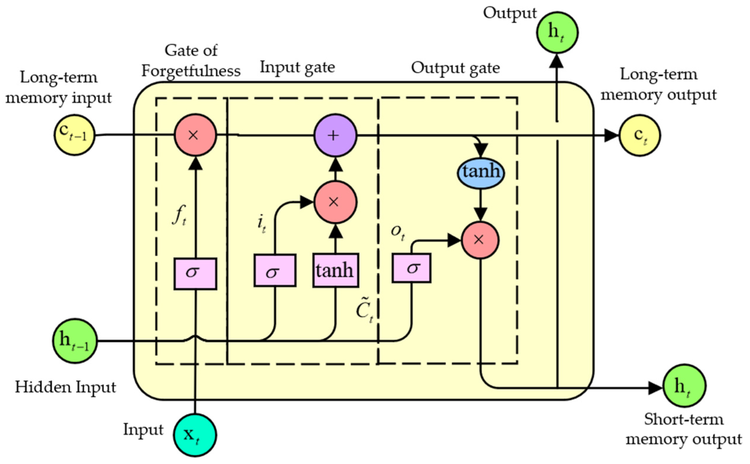
To address the nonlinear temporal characteristics of traction substation loads, an LSTM is used with a gating mechanism composed of a forget gate, input gate, and output gate to dynamically regulate information flow. The model structure is shown in Figure 6.
Figure 6.
LSTM model diagram.
The forget gate controls the extent to which historical memory is retained, while the input gate regulates the strength of updates to new features; together, they update the cell state Ct. The output gate generates the final output ht based on the current state. This mechanism effectively solves the vanishing gradient problem of recurrent neural networks(RNNs), and its core computation process is
where ft, it, ot are the outputs of the forget gate, input gate, and output gate; Ct is the cell state; ht is the hidden state; W and b are the weight matrices and bias terms corresponding to each gate; σ and tanh are the activation functions; ht−1 and xt are the concatenated vectors of the previous state and the current input; is the cell state of the current input.
3.4. Minimum Demand Control Strategy Based on Predictive Results
To validate the load forecasting algorithm, it was applied to the minimum demand control strategy of the traction substation. This strategy sequentially schedules the microgrid of the traction substation according to photovoltaic, wind power, energy storage, and the main grid [20]. When there is an excess of solar and wind power, the storage is charged, and when insufficient, it discharges, thereby reducing peak electricity purchases and lowering the substation’s demand on the grid.
During peak shaving, the system determines the high and low peak lines based on the mean and 1.5 times the standard deviation of the load forecast. When the load exceeds the ultra-peak line, the storage discharges until the state of charge (SOC) reaches 0.2; between the high and low peak lines, it discharges slightly to maintain the SOC at 0.6; below the low peak line, no discharge occurs. This strategy guides energy storage scheduling to reduce individual peak electricity purchases [21].
3.4.1. Objective Function
3.4.2. Constraint
During the optimization process, this model sets the following constraints to ensure the safety and stability of the energy storage system:
- (1)
- Charge and discharge power constraints
- (2)
- Charge and discharge mutual exclusion constraint
The charging and discharging power of the energy storage system is limited by its rated capacity, as shown in Equation (14), and it is subject to mutually exclusive conditions, as shown in Equation (15). This ensures that charging or discharging operations can only occur at one time. In addition, the SOC of the energy storage dynamically updates according to the actual energy conversion relationship, and its update process follows the equation:
where P is the charge/discharge power; is the duration of charge/discharge; is the charge/discharge efficiency; is the rated capacity of the energy storage system.
Meanwhile, the SOC is constrained by the lifespan protection boundary . Taking a 10 MWh energy storage system as an example, if the system discharges at 1 MW for 15 min, the SOC will drop by approximately 2.63%. Based on the above constraints, the minimum demand control strategy discharges at the maximum allowable operating power to shave peaks when the load exceeds the threshold, maintains SOC ≈ 0.6 between peak periods, and does not discharge during low-demand periods. This ensures the safe operation of the energy storage system while reducing the peak electricity purchases of the traction substation.
4. Case Analysis
4.1. Load Dataset
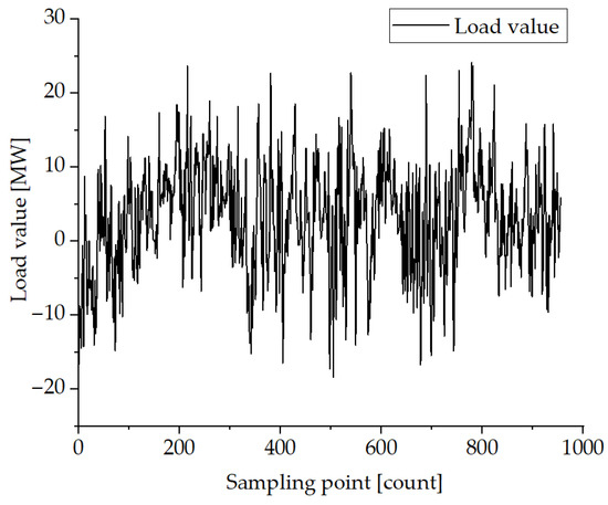
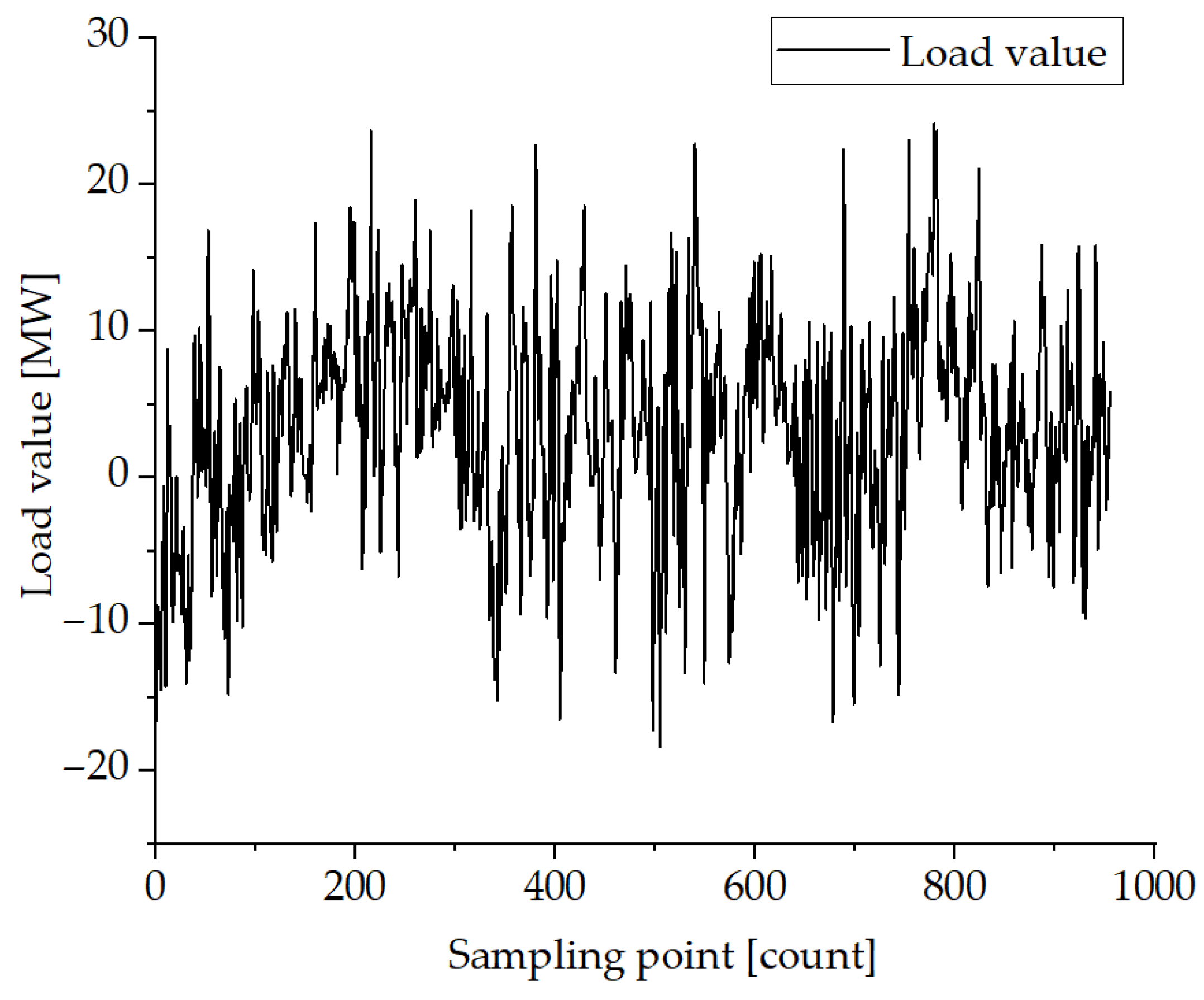
This study selected actual load data from a certain traction substation as the sample dataset, with data continuously collected at 15 min intervals over 10 days, resulting in 960 valid samples, as shown in Figure 7. Although the data duration is relatively limited, its high temporal resolution can clearly reflect the rapid fluctuations and short-term characteristics of traction loads, providing sufficient dynamic information for short-term forecasting models. In addition, this dataset meets the requirement of comparing the performance of different prediction models under consistent conditions, making it suitable as the benchmark data for this study.
Figure 7.
Towing station historical load sequence.
The positive and negative load of the traction substation is the sum of the train’s traction/braking power; positive load corresponds to the train’s overall braking and regenerative energy (which can be stored); and negative load corresponds to the train’s overall traction demand and additional power required. This is the net power flow between the substation and the train.
4.2. MOGWO-VMD-LSTM Prediction Simulation
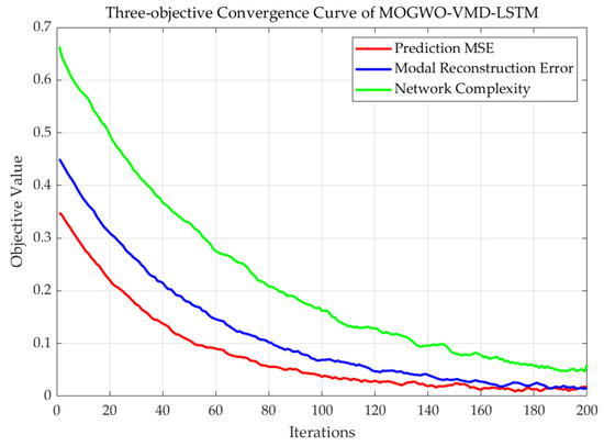
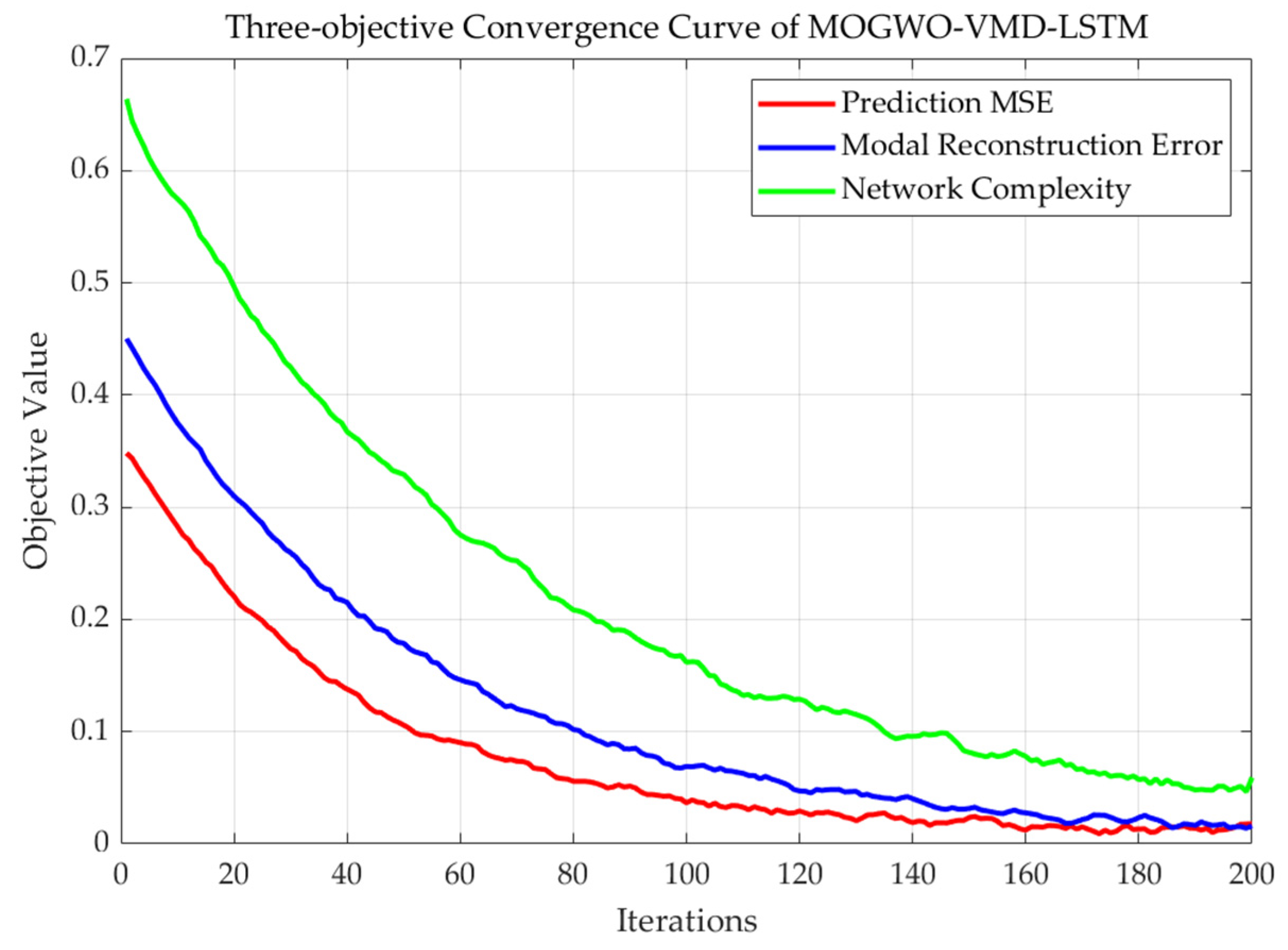
Figure 8 illustrates the convergence behavior of the multi-objective grey wolf optimizer during the joint optimization of VMD and LSTM parameters. The three objectives—prediction MSE, modal reconstruction error (MRE), and network complexity—are all minimized simultaneously. As the iteration progresses, all three objective values gradually decrease and stabilize, indicating that MOGWO successfully balances forecasting accuracy, decomposition quality, and model complexity.
Figure 8.
Convergence curves of the three-objective MOGWO.
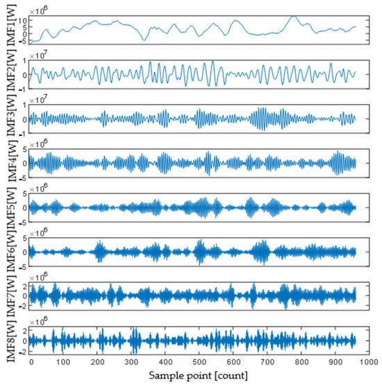
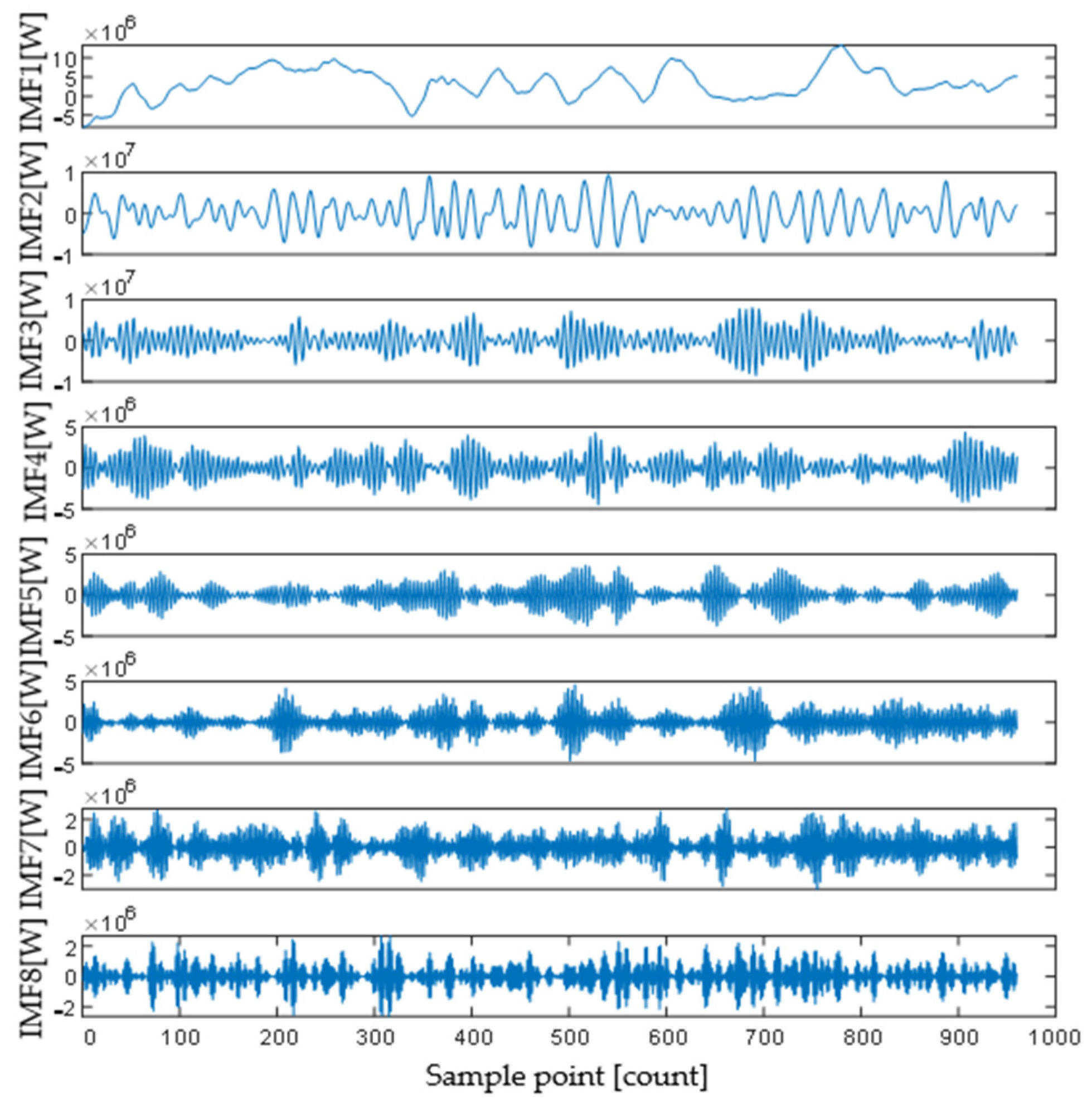
The optimal VMD key parameters obtained by MOGWO are as follows: the number of modal components K is 8, the bandwidth constraint penalty factor α is 1000 (the search ranges—VMD modal number K [8, 15] and penalty factor α [200, 2000]), there is no DC component (DC = 0), the initial center frequencies are uniformly distributed (init = 1), the convergence criterion tolerance tol is 10 × 10−9, and the noise tolerance τ is 0.02. The VMD decomposed modal components are shown in Figure 9.
Figure 9.
VMD load decomposition graph.
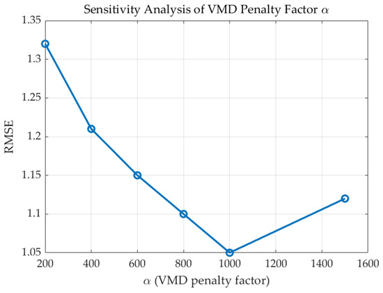
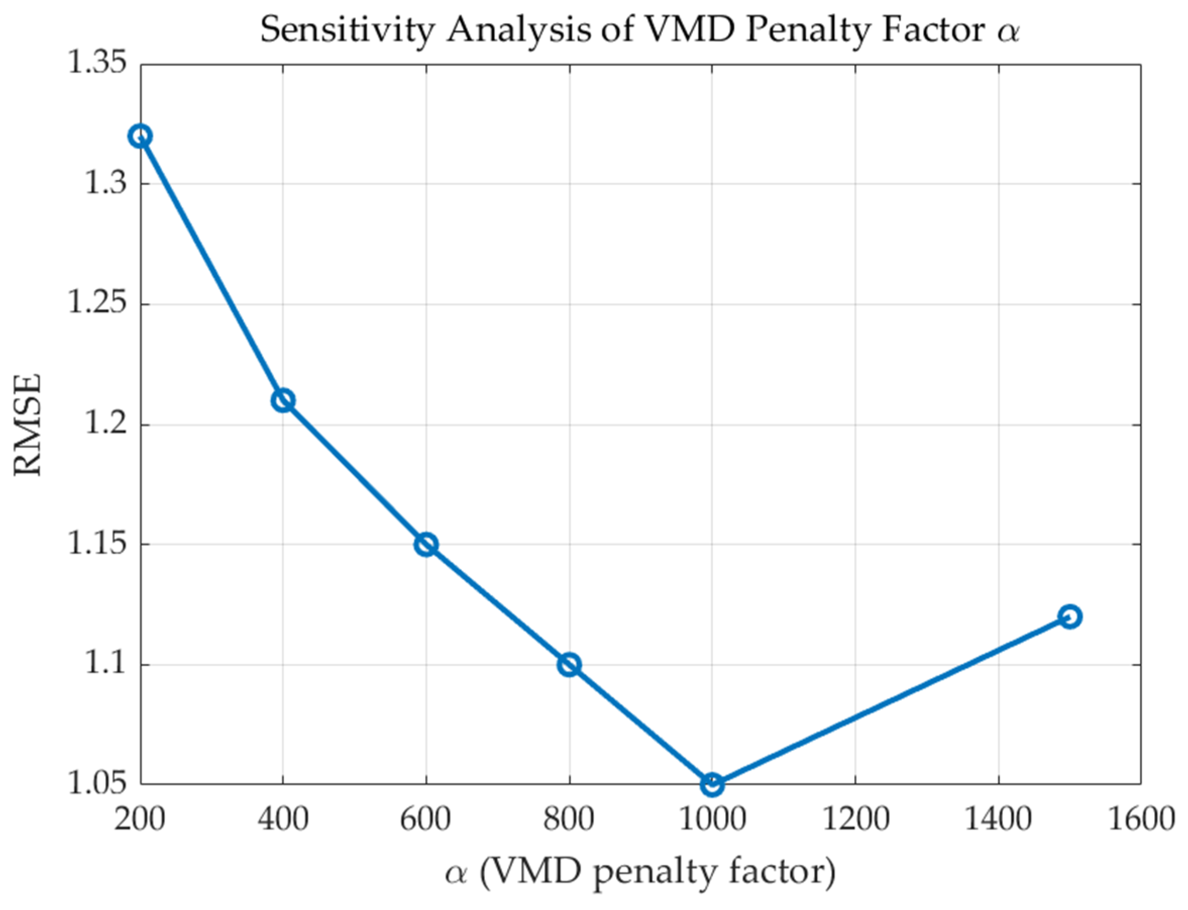
A lightweight sensitivity analysis was conducted on the penalty factor α of VMD. Using different α values, the root mean square error (RMSE) curve exhibited a clear convex shape, with the minimum occurring at approximately α ≈ 1000, indicating that the selected parameter is robust and not overly sensitive to minor perturbations. Sensitivity analysis of α is shown in Figure 10.
Figure 10.
Sensitivity analysis of α.
The hyperparameters obtained using the MOGWO optimization algorithm for this study are a 2-layer LSTM, 90 hidden neurons per layer, a dropout of 0.2, a learning rate of 0.005, a batch size of 64, a time window of 30 time steps, and a weight decay of 1 × 10⁻⁴. The search ranges for the parameters are set as follows: the number of hidden neurons between [80, 100], the learning rate between [0.001, 0.01], the maximum number of iterations between [500, 1000], the dropout rate between [0.1, 0.5], the batch size between [32, 128], the weight decay between [1 × 10⁻⁵, 1 × 10⁻³], and the time window between [20, 50]. These ranges are set based on constraints from similar studies to ensure a balance between model optimization efficiency and prediction performance.
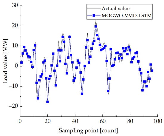
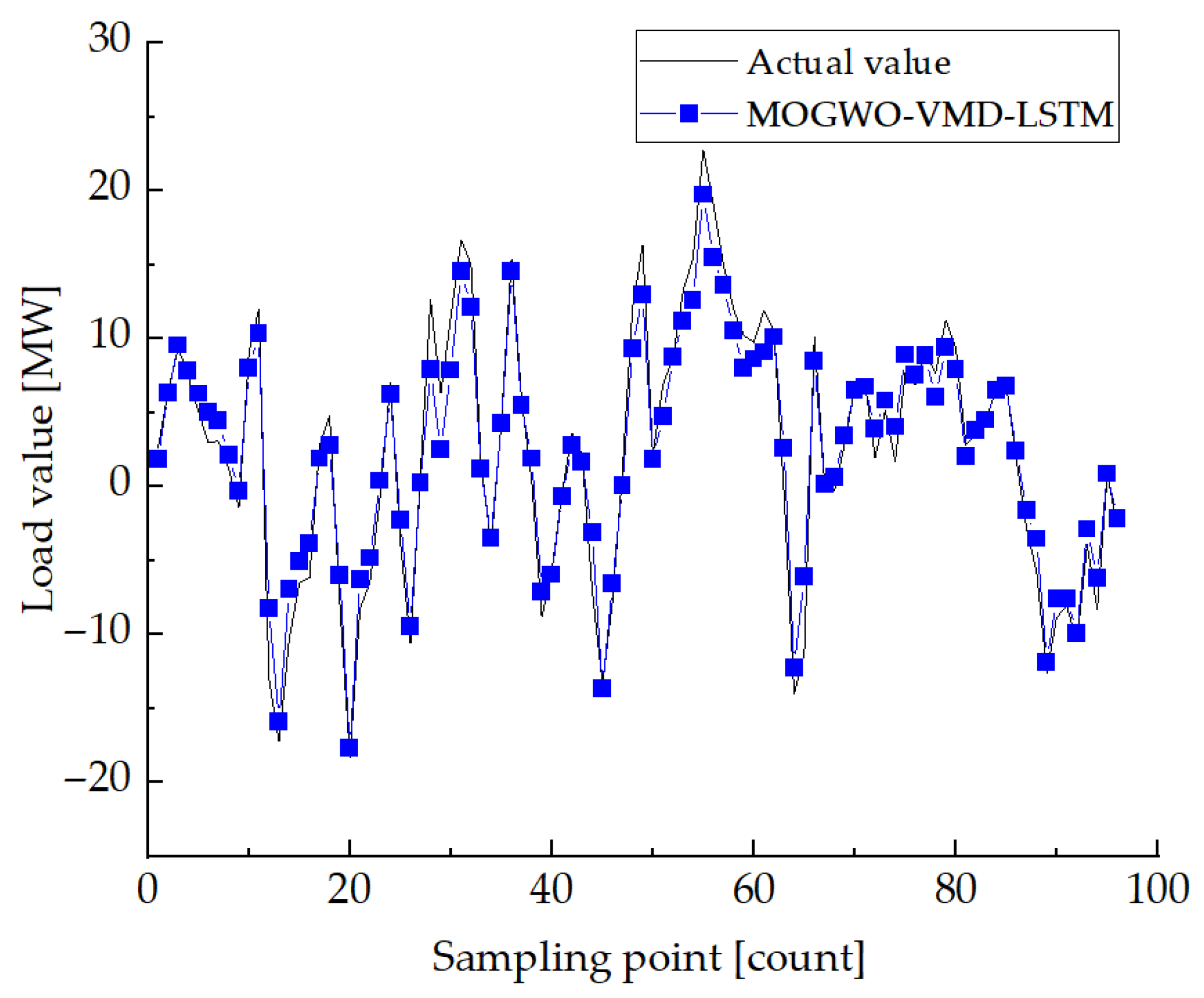
As shown in Figure 11, its overall prediction trend is highly consistent with the actual values, accurately capturing the load peaks and troughs.
Figure 11.
MOGWO-VMD-LSTM prediction results.
Table 3 shows a comparison of all selected parameters for the prediction models, including the number of layers, the number of units per layer, the optimizer, and the learning rate. These parameters come from empirical values and optimization.
Table 3.
Comparison of Parameter Settings of Various Prediction Models.
The number of LSTM layers in the proposed MOGWO-VMD-LSTM model is determined through the optimization process, while the other prior-model configurations—using only one layer—are mainly due to considerations of simplicity, computational efficiency, avoidance of overfitting, and consistency with commonly used benchmark settings.
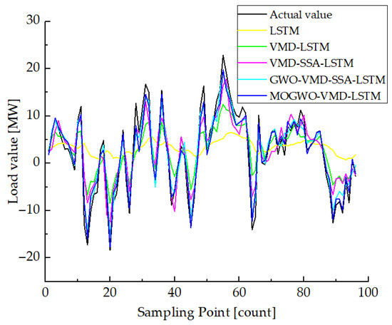
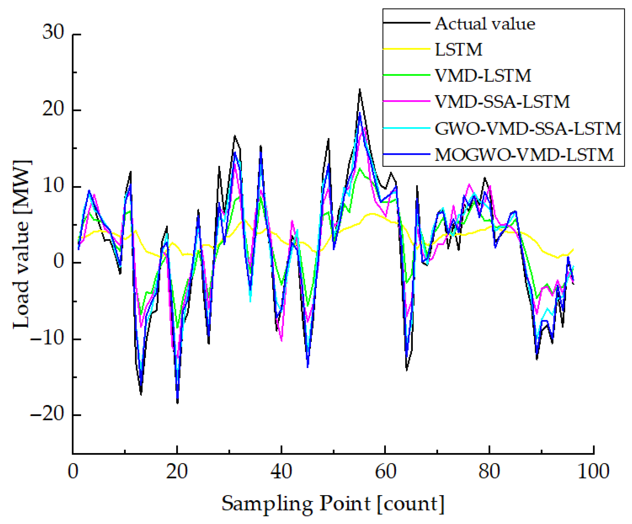
Figure 12 presents a comparison of the proposed algorithm with prediction algorithms such as LSTM, VMD-LSTM, VMD-SSA-LSTM, and GWO-VMD-SSA-LSTM. The results show that LSTM has low accuracy, while the MOGWO-VMD-LSTM predictions are closest to the actual values.
Figure 12.
Comparison of prediction results of different models.
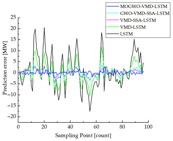
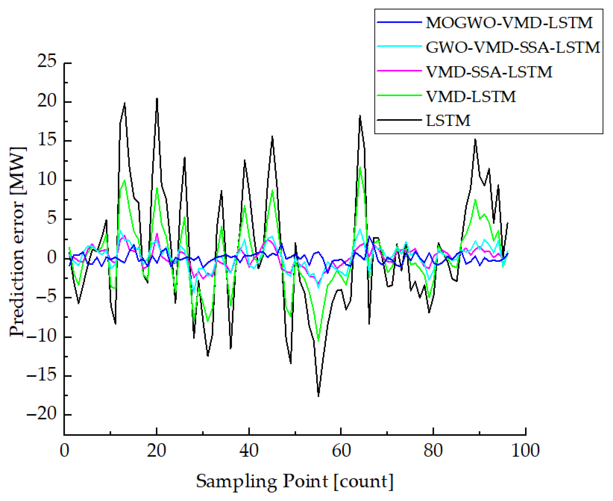
Figure 13 shows the comparison of model errors. The single LSTM has large and widely fluctuating errors, while the MOGWO-VMD-LSTM has the smallest and most stable errors, indicating that the proposed algorithm has higher load forecasting accuracy.
Figure 13.
Comparison of model prediction errors.
4.3. Evaluation Criteria
Forecast error analysis is a straightforward way to compare the prediction accuracy of different models. The following common indicators are often used in electric load forecasting.
- (1)
- Mean Absolute Error (MAE):
- (2)
- Root Mean Square Error (RMSE):
- (3)
- Mean Absolute Percentage Error (MAPE):
Table 4 shows the specific evaluation results of different models.
Table 4.
Model Evaluation Form.
Analysis shows that the performance of VMD-LSTM is significantly improved compared to a single LSTM, with RMSE, MAE, and MAPE significantly reduced, while the various errors of MOGWO-VMD-LSTM further decreased by 2.31%, 2.78%, and 7.52% compared to the suboptimal model GWO-VMD-SSA-LSTM, highlighting the advantage of MOGWO in collaboratively optimizing parameters.
As shown in Table 4, the proposed MOGWO-VMD-LSTM achieves the best overall accuracy. To ensure that this improvement is not due to randomness, ten independent runs were performed and the Wilcoxon signed-rank test confirmed that all p-values were below 0.05, indicating statistically significant gains (Detailed data can be found in Appendix A). In addition, the ablation analysis shows a consistent performance improvement from LSTM → VMD-LSTM → VMD-SSA-LSTM → GWO-VMD-SSA-LSTM → MOGWO-VMD-LSTM, demonstrating that VMD decomposition and MOGWO optimization contribute effectively to the final model performance.
4.4. Simulation of the Application of Load Forecasting Algorithms in Minimum Demand Control Strategies for Traction Stations
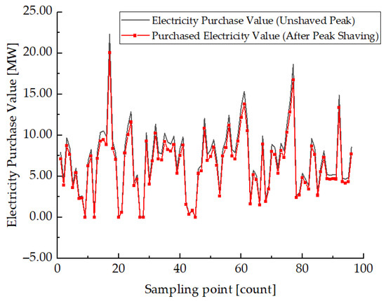
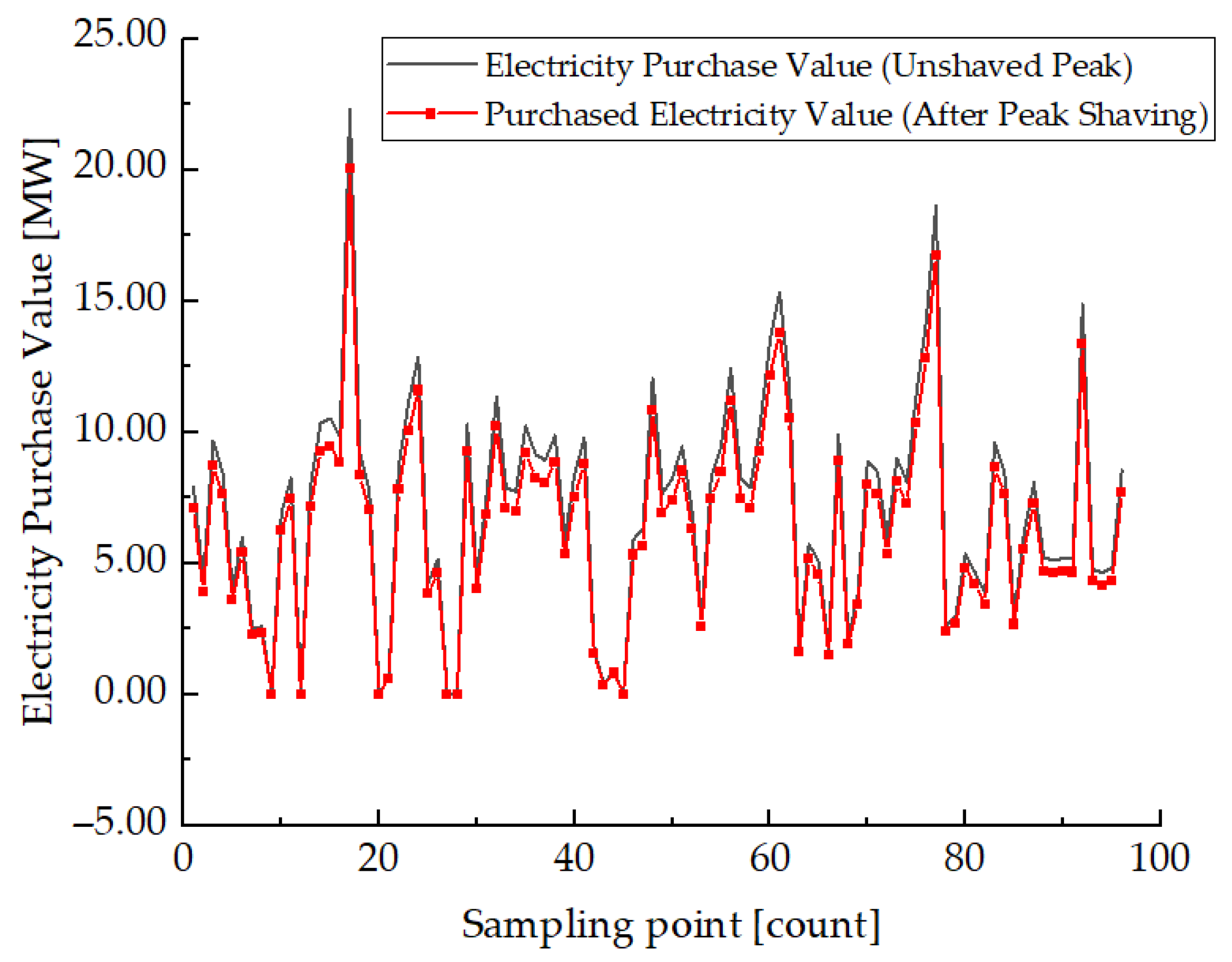
The minimum demand control strategy for the traction station divides the high and low peak lines based on the mean and 1.5 times the standard deviation of the load forecast results. When the load exceeds the high peak line, the energy storage discharges until the SOC reaches 20% and then stops; between the high and low peak lines, a slight discharge maintains the SOC at around 60%; no discharge occurs below the low valley line. Where SOC = 20% is usually considered the lower limit to avoid deep discharge and protect battery life, while SOC = 60% serves as the upper limit of the intermediate range that is safe and flexible for dispatch in many energy storage scheduling scenarios, ensuring there is still enough charge and discharge capacity to perform peak shaving tasks. The peak-valley boundary is set according to the statistical distribution of the load curves in this study’s dataset to ensure that the strategy can be effectively triggered within the actual load fluctuation range. The comparison of peak shaving results under this strategy is shown in Figure 14.
Figure 14.
Comparison chart of peak power purchase based on the forecast results.
This discharge strategy reduces the peak power purchase in a single instance from 22.279 MW to 20.052 MW, a decrease of 9.995%. It is evident that accurate load forecasting and reasonable energy storage scheduling can effectively alleviate the electricity purchasing pressure on the grid and improve the economic efficiency and reliability of energy management.
5. Conclusions
This study focuses on the minimum demand scheduling strategy of traction substations and constructs a MOGWO-VMD-LSTM collaborative prediction framework. Based on the load forecasting results, an energy storage charging and discharging strategy is implemented, leading to the following conclusions:
- (1)
- This study proposes a novel MOGWO-VMD-LSTM framework for load forecasting, in which the parameters of variational mode decomposition and long short-term memory networks are jointly optimized using a multi-objective strategy. By integrating decomposition and prediction parameters within a unified search space, the proposed method effectively mitigates the mismatch between single-module optimization and overall model performance. Experimental results in load forecasting scenarios demonstrate that the proposed coupling framework achieves higher accuracy than existing prediction models in terms of RMSE, MAE, and MAPE, thereby providing a new technical path for accurate time-series load prediction.
- (2)
- Applying the load forecasting results to guide practical energy storage charging and discharging reduces the peak power purchase from 22.279 MW to 20.052 MW, a decrease of 9.995%, effectively alleviating the power grid’s electricity purchase pressure.
- (3)
- While the proposed method demonstrates improved forecasting accuracy and peak-shaving performance, it does not fully address seasonal variations or anomalous conditions such as holidays or maintenance periods. Future research will aim to extend the framework to handle these scenarios, further enhancing its robustness and practical applicability.
Author Contributions
Conceptualization, X.L.; Methodology, X.L.; Software, X.L.; Validation, X.L., J.L. and T.Z.; Formal analysis, X.L.; Investigation, X.L., J.L. and T.Z.; Resources, X.L., Y.S. and C.D.; Data curation, X.L.; Writing—original draft, X.L.; Writing—review & editing, X.L., Y.S. and C.D.; Visualization, X.L.; Supervision, Y.S.; Project administration, X.L. and C.D.; Funding acquisition, X.L., Y.S. and C.D. All authors have read and agreed to the published version of the manuscript.
Funding
This research received no external funding.
Data Availability Statement
The original contributions presented in this study are included in the article. Further inquiries can be directed to the corresponding author.
Conflicts of Interest
The authors declare no conflict of interest.
Appendix A
This appendix provides supplementary experimental results to support the statistical analysis presented in the main text. Specifically, all experiments were conducted independently ten times using different random seeds. The performance metrics reported in Table 4 of the main text correspond to the average values of these ten independent runs.
The tables presented in this appendix are constructed based on the results of the ten runs and are used to perform the Wilcoxon signed-rank test, aiming to further evaluate the statistical significance of the performance differences between the proposed method and the comparison models. These supplementary results enhance the transparency and robustness of the experimental analysis. The Wilcoxon signed-rank test results indicate statistically significant differences (p < 0.05) between the proposed method and all comparison models across all evaluation metrics.
Table A1.
Wilcoxon Signed-Rank Test Results of MOGWO-VMD-LSTM and Other Comparison Models.
References
- Song, F.; Wang, L.; Zhang, X.Q.; Wang, Y.Z. Prediction of recurrent neural network and optimization of nash game behavior for multi-agent micro-grids. Trans. Electrotech. Soc. Power Syst. Autom. 2023, 35, 136–142. [Google Scholar]
- Tian, X.; Chen, L.J.; Li, X.Z.; Yuan, W.K. Optimal operation strategy for shared energy storage in distributed photovoltaic communities based on stackelberg game and improved shapley value. Power Syst. Technol. 2023, 47, 2252–2261. [Google Scholar]
- Guo, Y.X.; Li, Y.; Qiao, X.B.; Zhang, Z.; Zhou, W.; Mei, Y. BiLSTM multitask learning-based combined load forecasting considering the loads coupling relationship for multienergy system. Smart Grid 2022, 13, 3481–3492. [Google Scholar] [CrossRef] [Scilit]
- Cheng, L.L.; Zang, H.X.; Xu, Y.; Wei, Z.; Sun, G. Probabilistic residential load forecasting based on micrometeorological data and customer consumption pattern. Power Syst. 2021, 3, 3762–3775. [Google Scholar] [CrossRef] [Scilit]
- Hu, W.; Zhang, X.Y.; Li, Z.N. Short-term load forecasting based on the optimized VMD-mRMR-LSTM model. Power Syst. Prot. Control 2022, 50, 88–97. [Google Scholar]
- Yu, Y.; Wen, B.; Wang, Z.Y.; Mi, Z.Q.; Yuan, Y.B.; Chang, S.Q. Optimal scheduling of virtual power plants with uncertain sources and loads based on VMD and dual-mode EMPC. Acta Energ. Sol. Sin. 2023, 44, 130–138. [Google Scholar]
- Luo, X.Y.; Liu, J.; Yang, B.; Tan, T.; Chen, C.S.; Yang, J. Ultra-short-term wind power prediction based on improved osprey optimization algorithm and VMD-LSTM. Acta Energ. Sol. Sin. 2025, 46, 652–660. [Google Scholar]
- Xiao, L.X.; Zhang, Y.; Zhou, H.; Zhao, G.H. Ultra-short-term wind power forecasting based on IAOA-VMD-LSTM. Acta Energ. Sol. Sin. 2023, 44, 239–246. [Google Scholar]
- Wang, J.; Wang, J.H.; Cheng, K.; Fang, J.; Ju, D.Y. Rural ultra-short-term power load forecasting based on double-layer optimized VMD-LSTM. J. Shenyang Agric. Univ. 2024, 55, 92–102. [Google Scholar]
- Hu, R.; Qiao, J.F.; Li, Y.H.; Sun, Y.P.; Wang, B.B. Medium and long-term wind power forecasting based on WOA-VMD-SSA-LSTM. Acta Energ. Sol. Sin. 2024, 45, 549–556. [Google Scholar]
- Zhang, L.; Liu, J.C. Short-term load interval prediction method based on EEMD-SE and PSO-KELM. China Power 2021, 54, 132–140. [Google Scholar]
- Li, X.S.; Fang, Z.J.; Li, F.; Jie, S.J.; Cheng, S. Optimal scheduling of distribution network game with multi-microgrid leasing and shared energy storage. Proc. CSEE 2022, 42, 6611–6624. [Google Scholar]
- Xiao, J.W.; Liu, P.; Fang, H.L.; Liu, X.-K.; Wang, Y.-W. Short-term residential load forecasting with baseline-refinement profiles and bi-attention mechanism. Smart Grid 2024, 15, 1052–1062. [Google Scholar] [CrossRef] [Scilit]
- Wang, Z.; Zhang, H.; Yang, R.; Chen, Y. Improving model generalization for short-term customer load forecasting with causal inference. Smart Grid 2025, 16, 424–436. [Google Scholar] [CrossRef] [Scilit]
- Liu, W.Y.; Zhou, Y.S.; Zhou, W.Q.; Su, S.; Li, B.; Deng, K.J. Prediction of electric vehicle charging load in urban power grids considering heteroskedasticity. Autom. Electr. Power Syst. 2024, 48, 54–63. [Google Scholar]
- Tan, M.; Yuan, S.P.; Li, S.; Su, Y.; Li, H.; He, F. Ultra-short-term industrial power demand forecasting using LSTM based hybrid ensemble learning. Power Syst. 2020, 35, 2937–2948. [Google Scholar] [CrossRef] [Scilit]
- Neeraj; Mathew, J.; Behera, R.K. EMD-Att-LSTM: A data-driven strategy combined with deep learning for short-term load forecasting. J. Mod. Power Syst. Clean Energy 2021, 10, 1229–1240. [Google Scholar] [CrossRef] [Scilit]
- Qi, Y.X.; Fan, J.Y.; Wu, D.H.; Wang, J. Short-term power load forecasting based on a combination of similar days and BiLSTM. Control Theory Appl. 2024, 41, 2304–2314. [Google Scholar]
- Ren, J.J.; Wei, H.H.; Zou, Z.L.; Hou, T.T.; Yuan, Y.L.; Shen, J.Q.; Wang, X.M. Ultra-short-term power load forecasting based on CNN-BiLSTM-Attention. Power Syst. Prot. Control 2022, 50, 108–116. [Google Scholar]
- Du, C.; Yang, S.; Qiu, L.; Ma, J.; Fang, Y.; Rodriguez, J. A Cross-decoupled Current Harmonics Suppression Method for IPMSM Based on Notch Filter and Second-order Generalized Integrator. IEEE Trans. Power Electron. 2025, 40, 5715–5730. [Google Scholar] [CrossRef] [Scilit]
- Du, C.; Yang, S.; Qiu, L.; Wang, Y.; Feng, J.; Ma, J. A Deadbeat Predictive Current Harmonics Suppression Method for IPMSM Based on Quasi Proportional Resonant Control. IEEE Trans. Power Electron. 2024, 39, 14909–14922. [Google Scholar] [CrossRef] [Scilit]

Disclaimer/Publisher’s Note: The statements, opinions and data contained in all publications are solely those of the individual author(s) and contributor(s) and not of MDPI and/or the editor(s). MDPI and/or the editor(s) disclaim responsibility for any injury to people or property resulting from any ideas, methods, instructions or products referred to in the content. |
© 2025 by the authors. Licensee MDPI, Basel, Switzerland. This article is an open access article distributed under the terms and conditions of the Creative Commons Attribution (CC BY) license.