Short-Term Load Forecasting Based on Similar Day Theory and BWO-VMD

Abstract

Short-term power load forecasting at the regional level is essential for maintaining grid stability and optimizing power generation, consumption, and maintenance scheduling. Considering the temporal, periodic, and nonlinear characteristics of power load, a novel short-term load forecasting method is proposed in this paper. First, Random Forest importance ranking is applied to select similar days and a weighted eigenspace coordinate system is established to measure similarity. The daily load sequence is then decomposed into high-, medium-, and low-frequency components using Variational Mode Decomposition (VMD). The high-frequency component is predicted using the similar day averaging method, while neural networks are employed for the medium and low-frequency components, leveraging historical and similar-day data, respectively. This multi-faceted approach enhances the accuracy and granularity of load pattern analysis. The final forecast is obtained by summing the predictions of these components. The case study demonstrates that the proposed model outperforms LSTM, GRU, CNN, TCN and Transformer, with an RMSE of 660.54 MW and a MAPE of 7.81%, while also exhibiting fast computational speed and low CPU usage.

1. Introduction

Power load forecasting at the regional level is crucial for departments involved in power dispatch, consumption, and planning, as it significantly impacts the operation, planning, and dispatch of power grids across the entire region [1]. Power load forecasting is typically categorized into long-term, medium-term, and short-term forecasting, based on the different periods [2]. Short-term Load Forecasting (STLF) typically covers the next few minutes to a week. Accurate STLF aids in the optimal scheduling of generating units, consumption planning, and maintenance, thereby ensuring the grid’s safety and stability.

The integration of a large-scale renewable energy source adds complexity to the system, increasing the demand for precise STLF at both system and regional levels [3,4]. Power loads, influenced by human activities, weather, and other factors, exhibit temporality, periodicity, and nonlinearity, challenging accurate predictions [5]. Numerous studies have been conducted on regional-level STLF, with methods mainly including traditional and machine learning approaches [6,7]. Traditional forecasting methods like multivariate linear regression [8], Support Vector Regression (SVR) [9], autoregression [10] and exponential smoothing [11], though simple and quick, struggle with nonlinear relationships. In recent years, machine learning methods have gained increasing application due to their ability to handle nonlinearity. Reference [12] employs Random Forest (RF) Regression to predict groundwater, demonstrating excellent forecasting performance compared to other regression models. In the application of neural networks for load forecasting, Convolutional Neural Networks (CNNs) can extract features from data and accurately handle nonlinear sequences [13] but may compromise the continuity of power load as a time series [14]. Advanced models like Long Short-Term Memory (LSTM) [15] and Gate Recurrent Units (GRU) [16] are widely used due to their temporal structure-based design. Recently, Transformer has been introduced into load forecasting as a sequence-to-sequence deep model architecture [17].

In recent years, hybrid methods have been increasingly applied to short-term forecasting. Reference [18] combines CNN and LSTM and applies this model to the power system in Bangladesh. The results confirm higher accuracy in load forecasting compared to non-hybrid models. Reference [19] combines CNN and Transformer for load forecasting, demonstrating its superiority over individual models. However, neural networks have the drawbacks of high computational complexity, slow convergence, and having local minima [20,21]. Therefore, the combination of time-series analysis and neural networks has been introduced.

References [22,23] propose the combination of similar day theory and neural network for STLF. The similar day theory selects historical days with similar characteristics to the forecasted day, which can help the model to find days that are more similar to the load sequence of the forecasted day thus improving the prediction accuracy [24,25]. Notably, extracting key features and identifying links between features are the focus of similar day theory. Reference [26] notes that similar days have the same weekday index and weather similar to the forecasted day. Reference [27] highlights the impact of renewable energy on the power grid. In load forecasting, incorporating the generation of renewable energy as features can also improve prediction accuracy. Reference [28] identifies similar days using Euclidean distance. Reference [29] integrates K-means clustering with the similar day theory, employing a weighted Euclidean distance to identify similar days. Reference [30] proposes a machine learning-based approach for similar day selection. In some studies, combining RF with weighted Euclidean distance has been shown to enhance the interpretability of similar day selection [31,32].

However, similar day theory may not be suitable for all load sequences under varying frequencies. Some other models introduce signal decomposition methods to extract key features and reduce model complexity [33]. Empirical Mode Decomposition (EMD) [34] is utilized to decompose and reconstruct the load sequence to capture the characteristics. Similar methods are Ensemble Empirical Mode Decomposition (EEMD) [35] and Variational Mode Decomposition (VMD) [36]. They can all be used in combination with ANNs. Among them, VMD is superior to other methods in dealing with signal non-stationarity [37]. Since VMD requires manual parameter setting, it is necessary to optimize these parameters. Reference [38] proposes the Greylag Goose Optimization (GGO) algorithm inspired by the V-formation flight of geese and demonstrates superior accuracy over other algorithms in both benchmark tests and engineering applications. Similarly, the Grey Wolf and Dingo Optimization (GWDTO) algorithm combines the cooperative hunting strategy of Grey Wolf Optimization (GWO) with the dynamic search behavior of Dingo Optimization (DTO), effectively balancing exploration and exploitation [39]. The hybrid approach of Particle Swarm Optimization and Al-Biruni Earth Radius (PSO-BER) optimization leverages the fast convergence of PSO and the local refinement ability of BER, achieving competitive results in high-dimensional spaces [40]. However, the Beluga Whale Optimization (BWO) algorithm, inspired by the behaviors of beluga whales, demonstrates outstanding performance across 30 benchmark functions, surpassing 15 other metaheuristic algorithms in scalability and optimization accuracy [41]. Given its strong exploration and exploitation balance, as well as its global convergence capabilities, BWO shows great potential for optimizing Variational Mode Decomposition (VMD) in complex real-world applications [42].

Although hybrid models often improve prediction accuracy, they also introduce challenges related to computational efficiency. STLF is typically applied in real-time scheduling and management of power systems. To make timely adjustments, the model must be able to complete computations within a short time frame [43]. Reference [44] compares the computation time and CPU usage of various hybrid models to select the ones with higher computational efficiency.

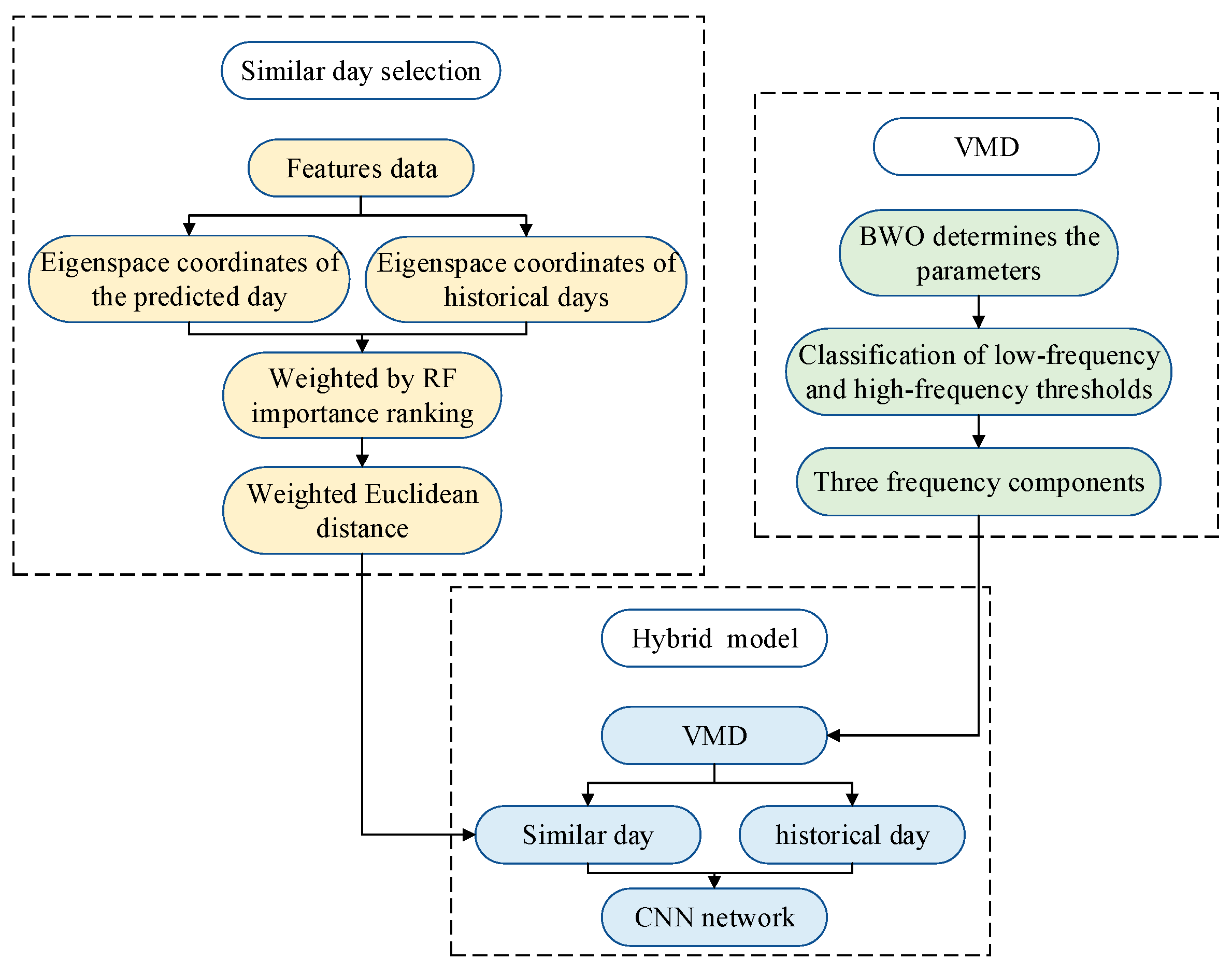
In this paper, a novel, efficient short-term load forecasting model based on similar day theory and VMD is proposed, which analyzes the 96-point load data of historical days and predicts the load sequence at 96 points for the next day. The contributions are summarized as follows:

(1) A weighted eigenspace coordinate system is proposed to select similar days. It uses Euclidean space and RF importance ranking to calculate similarity, which is then used to determine similar days. This similar day selection method improves the prediction accuracy of both medium-frequency and high-frequency components compared to the historical day-based method;

(2) The load sequence is decomposed using VMD algorithm, which is optimized by BWO. This is achieved by ensuring that the Intrinsic Mode Functions (IMFs) exhibit the lowest level of complexity, thereby making the trend and period of the decomposed sequence more distinct and recognizable by the forecasting model.

(3) A novel short-term load forecasting model combining similar day theory and VMD is proposed. By applying the similar day averaging method for high-frequency components and neural networks for medium- and low-frequency components, the model improves accuracy. Case studies demonstrate its superior performance compared to traditional methods.

The rest of this paper is organized as follows: Section 2 describes the methodology for similar day selection. Section 3 is the general flow of the proposed short-term load forecasting model combining similar day theory and VMD. In Section 4, a case study confirms the utility of the model. Section 5 concludes the paper. The general framework of this paper is shown in Figure 1.

2. Similar Day Selection

Traditional forecasting methods often use 1 day before, 2 days before, and 7 days before the forecasted day as inputs, but they are not necessarily the day closest to the forecasted day [45]. It is found that similar temperature, humidity, and tariff conditions produce similar load sequences. Therefore, this section describes the method of selecting similar days for the forecasting models.

2.1. Feature Processing

Due to the different resolutions of load data, this section considers daily features to accommodate inputs from various datasets. Since the units of the features differ, they must first be normalized to ensure consistency. The normalization process employs min–max normalization to achieve this:

$$x_j={\displaystyle \frac{{\widehat{x}}_j-{\widehat{x}}_{j\min }}{{\widehat{x}}_{j\max }-{\widehat{x}}_{j\min }}}$$

(1)

where ${\widehat{x}}_j$ is the value of feature j. Features can include maximum temperature, average temperature, humidity, electricity prices, atmospheric pressure, weekday index, etc., depending on the dataset. Also, the last moment load, first moment load and peak load of the historical day can be selected as features.

2.2. Feature Weight Determination

In order to analyze the effect of each feature on the similarity of daily load sequences, the RF importance ranking method is adapted.

RF first selects samples from the sample set to form a training set using bootstrap sampling and then constructs a decision tree based on the training set obtained through this sampling process. At each node of the tree, h features are selected randomly and without repetition. These h features are used to partition the training set in order to identify the optimal splitting feature, which can be evaluated using the Gini coefficient, gain ratio, or information gain. The Gini coefficient is defined as:

$$G{I}_q={\displaystyle \sum _{s=1}^S{\widehat{p}}_{qs}(1-{\widehat{p}}_{qs})}$$

(2)

where S is the number of categories in the training set and ${\widehat{p}}_{qs}$ is an estimate of the probability that a sample of node q belongs to class s.

The above steps are then repeated k times, where k represents the number of decision trees in RF. The test samples are predicted using the trained RF, and the final result is determined through a majority voting method.

In this paper, the Gini coefficient is used to evaluate the importance scores of features, and the change in the Gini coefficient before and after the ith decision tree node q is branched by feature j is as follows:

$$VI{M}_{jq}^{(Gini)(i)}=G{I}_q^{(i)}-G{I}_l^{(i)}-G{I}_r^{(i)}$$

(3)

where $G{I}_q^{(i)}$ denotes the Gini coefficient of the pre-branching node q. $G{I}_l^{(i)}$ and $G{I}_r^{(i)}$ denote the Gini coefficient of the two new nodes l and r after branching. If the nodes where feature j appears in the decision tree and i are collectively referred to as set Q, then the importance score at tree i is

$$VI{M}_j^{(Gini)(i)}={\displaystyle \sum _{q\in Q}VI{M}_{jq}^{(Gini)(i)}}$$

(4)

Since there are k trees in the RF, the final importance score of the feature j is

$$w_j={\displaystyle \frac{1}{k}}{\displaystyle \sum _{i=1}^{k}VI{M}_j^{(Gini)(i)}}$$

(5)

The normalized importance scores are considered as the feature weights.

2.3. Weighted Eigenspace Coordinate System Construction

Once the values and weights of features have been determined, the weighted Euclidean distance can be calculated as follows:

$$di{s}_{mn}=\sqrt{{\displaystyle \sum _{j=1}^d{w}_j{(x_{mj}-x_{nj})}^2}}$$

(6)

It is defined as similarity and when it is smaller, it means that two days are more similar.

The similarity is represented in the spatial coordinate system as shown in Figure 2. The black dashed line corresponds to the eigenspace coordinate system and d coordinate axes are established for d features, respectively. The coordinate on the feature j axis is $x_j$. The daily feature coordinate points corresponding to all features on day m and day n are $b_m^{\prime }(x_{m1},x_{m2},\dots ,x_{md})$ and $b_n^{\prime }(x_{n1},x_{n2},\dots ,x_{nd})$. The orange dashed line is the weighted eigenspace coordinate system with weights of w_j, corresponding to the daily feature coordinate points $b_m\left(w_1{x}_{m1},w_2{x}_{m2},\dots ,w_d{x}_{md}\right)$ and $b_n\left(w_1{x}_{n1},w_2{x}_{n2},\dots ,w_d{x}_{nd}\right)$. The distance between two points measures the similarity of features between two days.

3. Short-Term Load Forecasting Based on Similar Day Theory and BWO-VMD

3.1. BWO Algorithm

The BWO algorithm is an optimization algorithm inspired by the population behavior of beluga whales. The algorithm contains three phases: exploration, exploitation, and whale fall.

A population consisting of beluga whales can be represented as follows:

$$X=\left[\begin{array}{cccc}{x}_{1,1}& x_{1,2}& \dots & x_{1,t}\\ x_{2,1}& x_{2,2}& \dots & x_{2,t}\\ ⋮& ⋮& ⋮& ⋮\\ x_{n,1}& x_{n,1}& \dots & x_{n,t}\end{array}\right]$$

(7)

where n is the population size of beluga whales and t is the dimension of the variable to be optimized. The fitness function of beluga whales can be expressed as follows:

$$F_X=\left[\begin{array}{c}f[\begin{array}{cccc}{x}_{1,1}& x_{1,2}& \dots & x_{1,t}\end{array}]\\ f[\begin{array}{cccc}{x}_{2,1}& x_{2,2}& \dots & x_{2,t}\end{array}]\\ ⋮\\ f[\begin{array}{cccc}{x}_{n,1}& x_{n,2}& \dots & x_{n,t}\end{array}]\end{array}\right]$$

(8)

The location of the beluga whale can be considered as a search agent, which follows a random initialization approach:

$$X_{i,j}=l_{bj}+(u_{bj}-l_{bj})\times r$$

(9)

where u_bj and l_bj are upper and lower bounds on the variable, and are random numbers in the range (0, 1). In addition, beluga whales transition from the exploration phase to the exploitation phase by balancing factors $B_f$.

$$B_f=B_0(1-{\displaystyle \frac{g}{2G_{\max }}})$$

(10)

where B₀ is a random number between (0, 1), g is the current iteration number, and G_max is the maximum iteration number. When B_f > 0.5, the beluga whale is in the exploration phase, it swims in mirror image; when B_f < 0.5, it is in the exploitation phase, it engages in predatory behavior.

(1) Exploration phase: The position of the search agent is determined by the swimming of a pair of beluga whales, whose positions are updated as follows:

$$\left\{\begin{array}{c}{X}_{i,j}^{g+1}=X_{i,p_j}^g+(X_{i,p_1}^g-X_{i,p_j}^g)(1+r_1)\sin (2\pi r_2),j=even\\ X_{i,j}^{g+1}=X_{i,p_j}^g+(X_{i,p_1}^g-X_{i,p_j}^g)(1+r_1)\cos (2\pi r_2),j=odd\end{array}\right.$$

(11)

where $X_{i,j}^{g+1}$ is the new position of the ith beluga whale in the jth dimension, $X_{r,p_1}^g$ and $X_{i,p_j}^g$ are the current position of the rth and ith beluga whale (r is random), r₁ and r₂ are random numbers in the range (0, 1), and $\sin (2\pi r_2)$ and $\cos (2\pi r_2)$ are the random numbers used for averaging the fins across.

(2) Exploitation phase: The Levy flight strategy is introduced in the exploitation phase of BWO to capture prey, and its mathematical model of predation is represented as follows:

$$X_i^{g+1}=r_3{X}_{best}^g-r_4{X}_i^g+C_1\cdot L_F(X_r^g-X_i^g)$$

(12)

where $X_i^g$ and $X_r^g$ are the current position of the ith and rth beluga whale (r is random), $X_i^{g+1}$ is the new position of the ith beluga whale, $X_{best}^g$ is the best position among the beluga whales, and r₃ and r₄ are random numbers in the range (0, 1). $C_1=2r_4(1-g/G_{\max })$ is used to measure the strength of random jumps in the intensity of Levy flight. The computation of $L_F$ is as follows:

$$\left\{\begin{array}{c}{L}_F=0.05\times {\displaystyle \frac{u\times \sigma }{|v{|}^{1/\beta }}}\\ \sigma ={\left({\displaystyle \frac{\Gamma (1+\beta )\times \sin (\pi \beta /2)}{\Gamma [(1+\beta )/2]\times \beta \times 2^{(\beta -1)/2}}}\right)}^{1/\beta }\end{array}\right.$$

(13)

where $u$ and $v$ are normally distributed random numbers and $\beta$ is a constant that defaults to 1.5.

(3) Whale fall phase: The location of the beluga whale is updated as:

$$X_i^{g+1}=r_5{X}_i^g-r_6{X}_i^g+r_7{X}_{step}$$

(14)

where r₅, r₆ and r₇ are random numbers in the range (0, 1), $X_{step}=(u_b-l_b)\exp (-C_{2}g/G_{\max })$ is the step size of the whale fall, $C_2=2W_f\times n$ is the step factor, and u_b and l_b are upper and lower bounds on the variables. The probability of a whale fall is designed as a linear function:

$$W_f=0.1-0.05{\displaystyle \frac{g}{G_{\max }}}$$

(15)

The probability of a whale fall decreases from 0.1 in the initial iteration to 0.05 in the last iteration.

3.2. VMD

VMD is an adaptive signal decomposition method that effectively handles non-smooth and nonlinear signals. By iteratively identifying variational modes, the original time series is decomposed into several IMFs with limited bandwidth. The algorithm mainly includes the construction of the variational problem and the solution of the variational problem. The solution process of VMD mainly contains two constraints: (1) the sum of the bandwidths of the center frequencies of each IMF is required to be minimized; (2) the sum of all IMFs is equal to the original signal.

The VMD algorithm defines the IMF for a finite bandwidth with stringent constraints, which is shown in (16).

$$u_k(t)=A_k(t)\cos ({\varphi }_k(t))$$

(16)

where k is the number of IMFs set in advance.

(1)

Construction of the variational problem

To construct the variational problem, the transient zero-sequence current signal $[\delta (t)+j/\pi t]\ast u_k(t)$ is Hilbert transformed to obtain an analyzed signal with k IMFs and a one-sided spectrum:

$$\left\{[\delta (t)+{\displaystyle \frac{j}{\pi t}}]\ast u_k(t)\right\}{e}^{-j{w}_{k}t}$$

(17)

where $\delta (t)$ is the impulse function and $\ast$ denotes the convolution operation.

After computing the squared paradigm of (16) and estimating the bandwidth of each IMF, the variational problem is constructed as follows:

$$\left\{\begin{array}{c}\min \left\{{{\displaystyle \sum _{k=1}^K‖{\partial }_t\{[\delta (t)+\frac{j}{\pi t}]\ast u_k(t)\}{e}^{-j{w}_{k}t}‖}}_2^2\right\}\\ s.t.{\displaystyle \sum _{k=1}^K{u}_k=f}\end{array}\right.$$

(18)

(2)

Solution of the variational problem

In order to transform the above constrained variational problem into an unconstrained variational problem, a quadratic penalty factor $\alpha$ and a Lagrange multiplier operator $\lambda$ are introduced in (17), and the extended Lagrange expression is:

$$\begin{array}{l}L(\{u_k\},\{w_k\},\lambda )=\\ \alpha {{\displaystyle \sum _{k=1}^K‖{\partial }_t\{[\delta (t)+\frac{j}{\pi t}]\ast u_k(t)\}{e}^{-j{w}_{k}t}‖}}_2^2+\\ {‖f(t)-{\displaystyle \sum _{k=1}^K{u}_k(t)}‖}_2^2+〈\lambda (t),f(t)-{\displaystyle \sum _{k=1}^K{u}_k(t)}〉\end{array}$$

(19)

It is solved by Alternate Direction Method of Multipliers (ADMM) using multiplicative operators:

$$\begin{array}{l}{\widehat{u}}_k^{n+1}(w)={\displaystyle \frac{\frac{{\widehat{\lambda }}^n(w)}{2}+\widehat{f}(w)-{\displaystyle \sum _{i=1}^k{\widehat{u}}_i^{n+1}(w)}-{\displaystyle \sum _{i=k+1}^K{u}_i^n(w)}}{1+2\alpha {(w-w_k^n)}^2}}\\ w_k^{n+1}={\displaystyle \frac{{\displaystyle {\int }_0^{\infty }w|{\widehat{u}}_k^{n+1}(w){|}^{2}dw}}{{\displaystyle {\int }_0^{\infty }|{\widehat{u}}_k^{n+1}(w){|}^{2}dw}}}\end{array}$$

(20)

where ${\widehat{u}}_k^{n+1}(w)$ is the wiener filter of the current signal, $^$ is the Fourier transform, $w_k^{n+1}$ is the center of gravity of the power spectrum of the current IMF, and n is the number of iterations.

In VMD, the number of decomposed components k and the quadratic penalty factor α are two important parameters optimized by BWO. An excessively large value of k can cause over-decomposition, while a value that is too small may lead to under-decomposition. Likewise, setting α too high can result in the loss of frequency band information, whereas setting it too low may introduce information redundancy.

To find the optimal values of k and α, the fitness function is defined as the minimum envelope entropy. Minimizing envelope entropy improves the separability and regularity of the decomposed modes, as lower entropy indicates less mode mixing and more concentrated intrinsic features in the signal. The envelope entropy $E_p$ of a zero-mean signal $x(j)$ can be expressed as:

$$\begin{array}{l}{E}_p=-{\displaystyle \sum _{j=1}^N{p}_j}\lg p_j\hfill \\ p_j=a(j)/{\displaystyle \sum _{j=1}^{N}a}(j)\hfill \end{array}$$

(21)

where $p_j$ is the normalized form of $a(j)$ and $a(j)$ is the envelope signal obtained by Hilbert demodulation of the signal $x(j)$.

3.3. Signal Reconstructing

When reconstructing the signal, in order to divide the signal into three components, high-frequency, medium-frequency, and low-frequency, it is necessary to calculate the center frequency of each IMF as well as to set the high-frequency threshold and the low-frequency threshold.

(1) Center frequency calculation: Considering that the samples collect data every 15 min, there are a total of 96 data points in a day. The sampling frequency should be 96 times a day, i.e., 1/900 Hz, and this value should be multiplied with the dimensionless center frequency in the VMD solving process, i.e., to achieve the center frequency in units of Hz.

(2) High-frequency threshold setting: The high frequency component usually corresponds to short-term fluctuations within a day. The high-frequency threshold may be set to correspond to fluctuations over a period of hours. The data show significant fluctuations every 2 h, so the high-frequency threshold can be set to correspond to a 2 h frequency, which can be calculated as follows:

$$f_{\max }={\displaystyle \frac{1}{2\times 3600}}=1.389\times {10}^{-4}\mathrm{Hz}$$

(22)

(3) Low-frequency threshold setting: The low frequency component usually corresponds to the long-term trend over the course of a day. In order to extract the main trend of the daily load sequence, then the low frequency threshold can be set to correspond to a 24 h frequency:

$$f_{\min }={\displaystyle \frac{1}{24\times 3600}}=1.157\times {10}^{-5}\mathrm{Hz}$$

(23)

3.4. CNN

The forecasting model uses CNN.

As shown in Figure 3, CNN mainly consists of input layer, convolutional layer, ReLU layer, pooling layer and full-connectivity layer. The model takes historical load data and features as inputs, extracts the features of the load through convolutional operation, and then reduces the computational complexity through a pooling layer. Finally, the full-connectivity layer converts the features into a one-dimensional structure, and finally outputs the predicted values. The core of CNN is the convolutional layer, which extracts the features of load through the convolutional kernel by performing the convolutional operation. The formula for the convolution kernel to extract features is:

$$c=f(X\ast W^n+b^n)$$

(24)

where n denotes the convolution kernel size, f denotes the activation function, X denotes the input sequence, * denotes the convolution operation, W denotes the weights, and b denotes the bias vector.

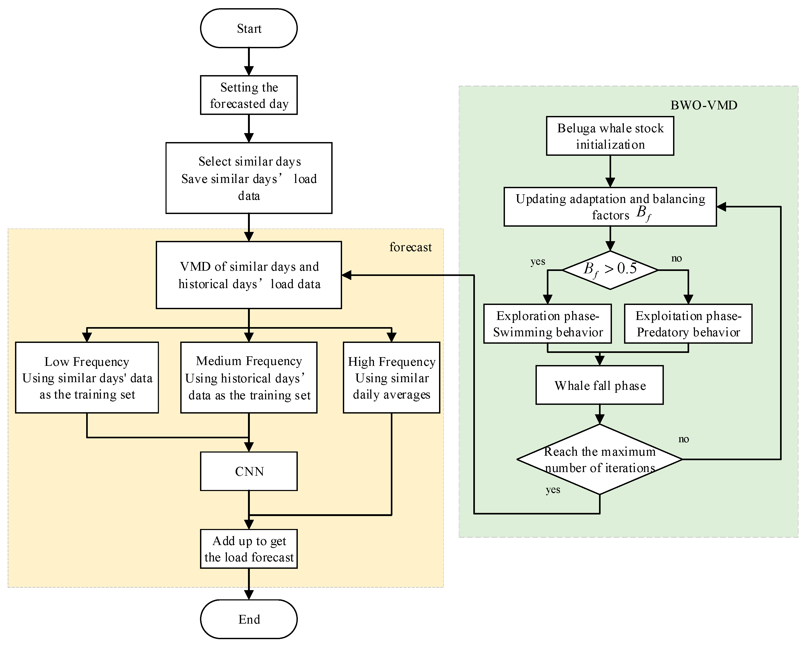
By integrating the aforementioned processes, the workflow of the short-term load forecasting model based on the similar-day theory and VMD is obtained, as illustrated in Figure 4.

The load forecasting model developed in this section first decomposes the daily load sequences using the VMD method. Two parameters of VMD, namely the number of decomposed components k and the quadratic penalty factor $\alpha$, are determined by BWO algorithm. Subsequently, the decomposed signals are categorized into high-frequency, medium-frequency, and low-frequency components based on their respective frequency ranges.

The low-frequency component captures the long-term trend. Power loads with similar climatic conditions and weekday indices exhibit comparable trends within a day, so the training set uses data from similar days. The medium-frequency component mainly reflects fluctuations and is strongly correlated with historical days. Therefore, the training set utilizes data from historical days. The high-frequency component is primarily composed of noise and interference, which is difficult to predict, so a similar day averaging method is employed.

Finally, the three components are summed to obtain the predicted load.

4. Case Study

In this paper, the daily 96-point load of a region in China from 1 January 2012 to 31 December 2014 is selected to be analyzed and predicted [46]. Additional experimental details can be found in the Supplementary Materials.

4.1. Evaluation Criteria

The indicators for evaluating the forecasting model are usually selected as MSE, RMSE, MAE, MAPE, etc. Using a variety of forecasting models, the goodness of the forecasting model can be evaluated by using these indicators as the evaluation criteria. RMSE focuses on the impact of large errors, while MAPE provides a normalized and easily interpretable error measure. Therefore, using these two indicators together helps to comprehensively evaluate the model’s performance.

RMSE is the Root Mean Square Error, which increases as the error becomes larger. It is defined as follows:

$$RMSE=\sqrt{{\displaystyle \frac{1}{n}}{{\displaystyle \sum _{i=1}^n\left({\widehat{y}}_i-y_i\right)}}^2}$$

(25)

RMSE’s range is $[0,+\infty ]$, when the error is larger, the value is larger.

MAPE is the Mean Absolute Percentage Error, as shown in (25).

MAPE’s range is $[0,+\infty ]$. A MAPE of 0% indicates a perfect model, and the larger the error, the larger the value.

$$MAPE={\displaystyle \frac{100\%}{n}}{\displaystyle \sum _{i=1}^n\left|\frac{{\widehat{y}}_i-y_i}{y_i}\right|}$$

(26)

In addition to MAPE and RMSE, this study incorporates computation time and CPU usage as additional evaluation criteria. These indicators provide a more comprehensive assessment of model performance, especially when dealing with large datasets or real-time forecasting applications. While accuracy is critical, the computational efficiency of a model is equally important for practical deployment, particularly in power systems where timely adjustments need to be made.

4.2. Data Preprocessing

The data includes load data and feature data. First, the weekday indexes are obtained from the official website of perpetual calendar. And then the weights of the features are determined according to the existing data. The results are shown in

Table 1. The importance of features.

Features	Importance
Maximum temperature (°C)	0.12
Minimum temperature (°C)	0.26
Average temperatures (°C)	0.34
Relative humidity (%)	0.09
Precipitation (mm)	0.03
Weekday index	0.15

.

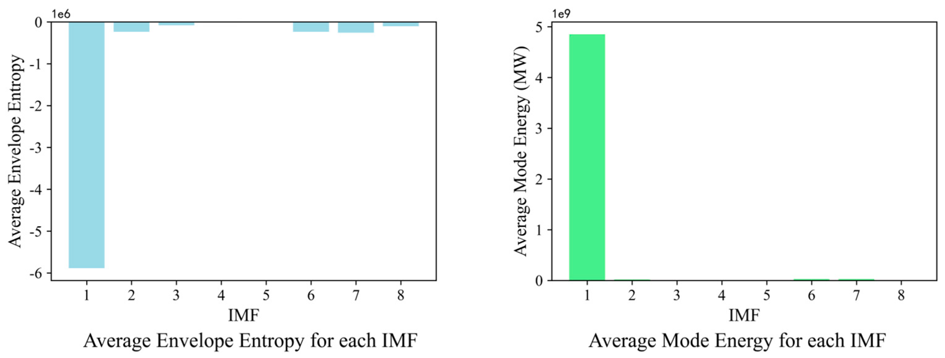
The 96-point load data of all days are decomposed with the BWO-VMD. The optimized number of decomposed sequences is 8, and the penalty coefficient is 50. To verify the validity of the parameters selected by BWO, a sliding window method is used to calculate the average envelope entropy and average energy for each IMF, as shown in Figure 5. From Figure 5, it can be observed that the low-frequency components exhibit lower envelope entropy and higher energy, indicating that these modes effectively capture the main trend components of the signal. In contrast, the high-frequency components show higher envelope entropy and lower energy, suggesting that they primarily capture the high-frequency fluctuations or noise in the signal. Overall, the VMD effectively extracts different frequency band information from the signal, validating the reasonableness of the VMD parameters optimized by BWO.

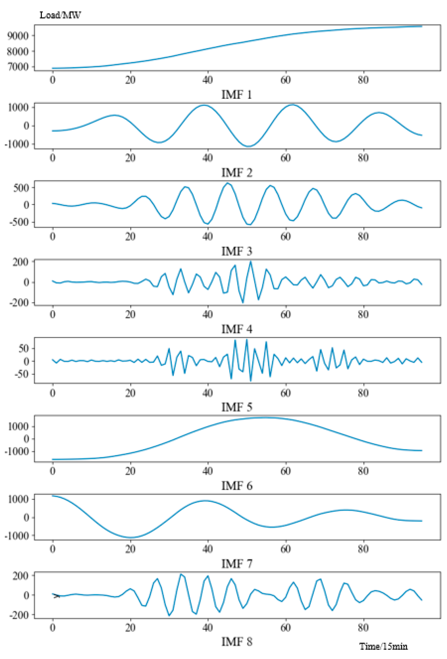
The VMD results of the forecasted day, taking 6 August 2013, as a case, are shown in Figure 6.

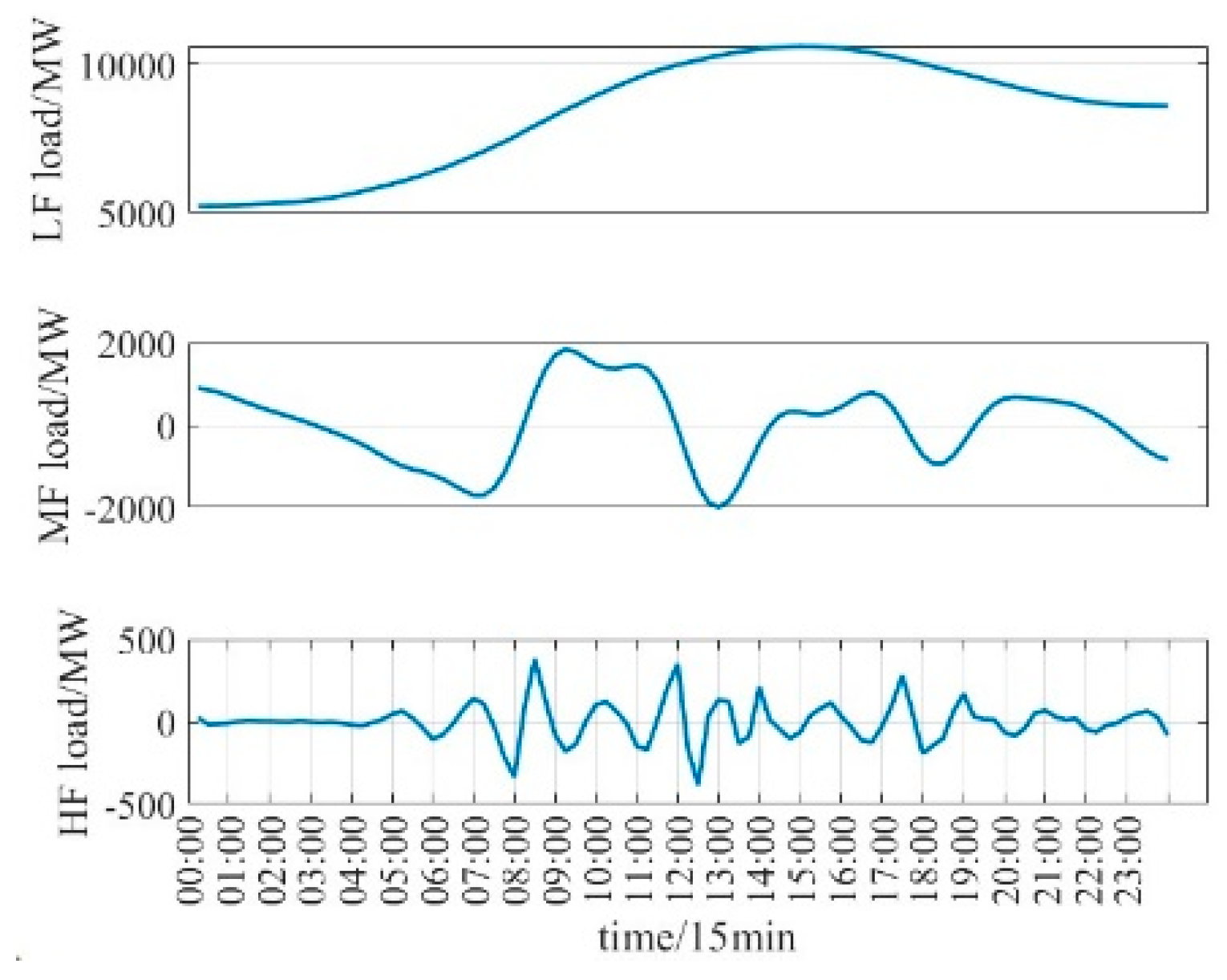
As shown in Figure 7, The eight IMFs are sorted according to the spectrogram, and the IMFs are classified into high-frequency, medium-frequency, and low-frequency components according to the set of high-frequency threshold and low frequency threshold. The decomposed curves of high-, medium-, and low-frequency components reveal distinct patterns that contribute differently to the overall prediction accuracy. The low-frequency component clearly captures the long-term trend of the daily load, offering stable and smooth variations that are critical for accurate baseline prediction. The medium-frequency component reflects more localized fluctuations, which align well with historical daily patterns and enhance the model’s ability to track dynamic changes. In contrast, the high-frequency component exhibits irregular and noisy behavior, suggesting limited predictive value. Nevertheless, applying a similar day averaging method to this component helps to mitigate residual noise. These observations confirm that the decomposition not only improves interpretability but also plays a vital role in enhancing prediction performance, particularly through the contributions of the low- and medium-frequency components.

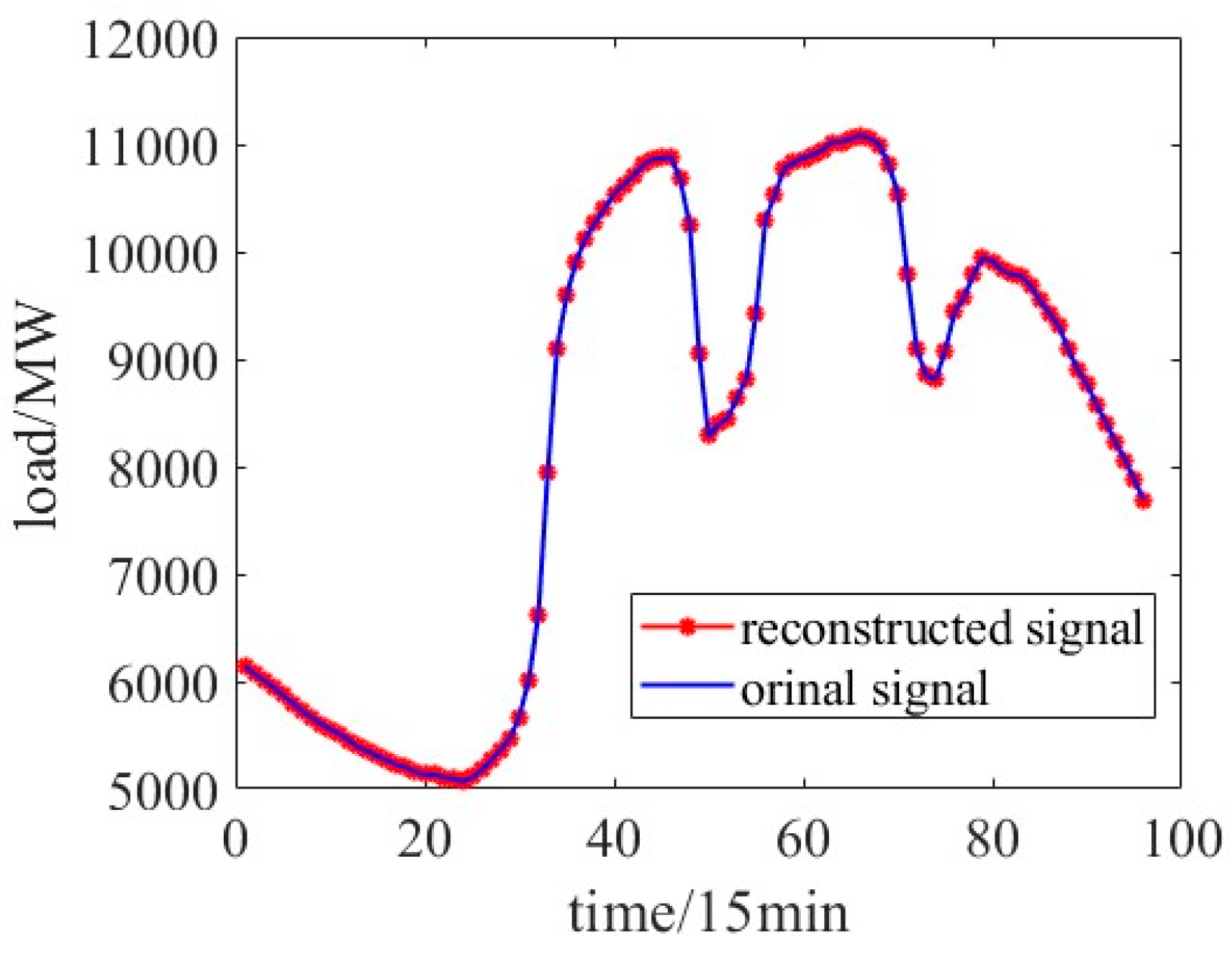
As seen in Figure 8, the VMD has residuals, and by calculation, the residuals are all below 0.1%, so they are not considered. All load sequences are reconstructed and saved as three data files.

4.3. Model Parameter Setting

(1)

Low frequency

The number of days used in the training set is denoted by q, the number of days to find similar days before the forecasted day is denoted by r, and the number of similar days to take is denoted by s. After an initial screening, q is selected as 60 or 90, r is selected as 10 or 20, and s is selected as 3 or 5. The test results are shown in

Table 2. Low-frequency training set’s parameters.

Parameters (q,r,s)	RMSE	MAPE
60, 10, 3	191.00	47.31
90, 10, 3	192.53	48.55
60, 20, 3	464.22	133.79
60, 10, 5	232.07	68.04

.

Finally, the training set is determined to be 60 days before the forecasted day, and three similar days are taken from the first 10 days of the day to be tested. The forecasting model is studied in terms of moment. In the training set, the input is the current moment load of similar days, and the output is the current moment of the forecasted day. In the test set, the input is the current moment load of similar days, and the output is the current moment of the forecasted day. A total of 96 forecasts are made to obtain a final 96-point load sequence of the forecasted day.

(2)

Medium frequency

The medium-frequency training set is empirically tested by taking 60, 90, and 120 days before the forecasted day. The number of days used in the training set is denoted by n, and the final results are shown in

Table 3. Medium-frequency training set’s parameters.

Parameter (n)	RMSE	MAPE
60	992.96	16.18
90	237.77	3.28
120	455.92	6.31

.

Based on the above results, it is finalized that the training set is 90 days before the forecasted day and the first 3 days before those forecasted are historical days. In the training set, the input is the current moment load of the historical day as well as the data of features of the historical day and the forecasted day, and the output is the current moment of the forecasted day. In the test set, the input is the current moment load of the historical day and the feature data of the historical day and the forecasted day, and the output is the current moment of the forecasted day.

(3)

High frequency

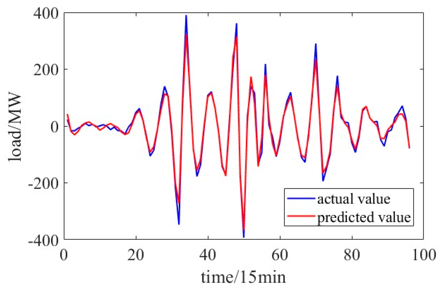
The high-frequency component averages the high-frequency components of the similar days according to the corresponding moments, and it finally adds them to the low frequency component as well as the medium frequency component to obtain the final prediction. In this case, the predicted and actual comparison of the high-frequency component using the similar day averaging method is shown in Figure 9.

As shown in Figure 9, the RMSE of the error between the predicted value and the true value in the high-frequency component is 20.08 MW, the error is relatively small, so the method is applicable.

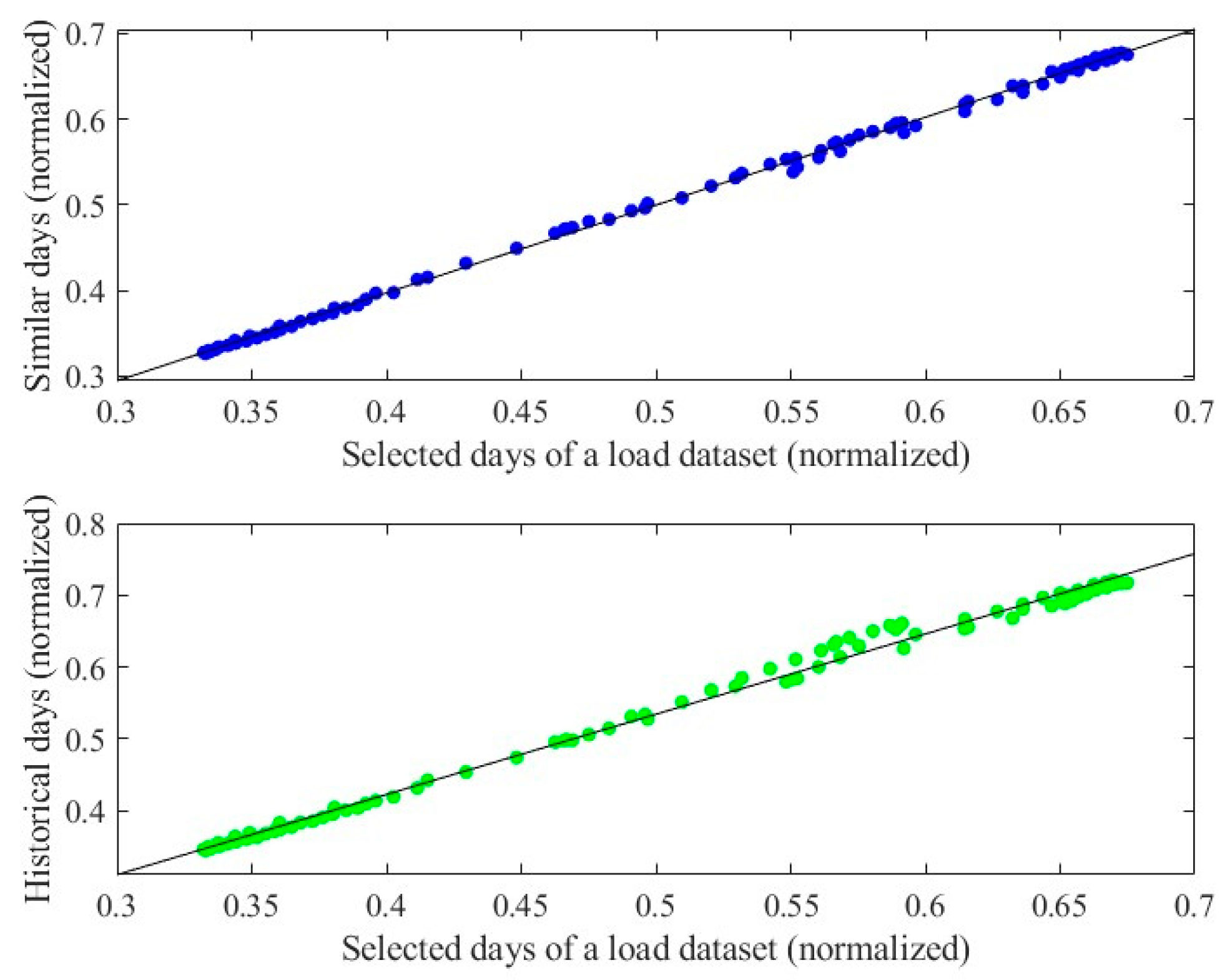
4.4. Performance of Similar Day Selection

Load data from 1 January 2014 to 31 December 2014 is taken to verify the superiority of similar day selection. The average results are shown in Figure 10 and

Table 4. Comparison of average correlation between similar and historical days.

Targets	Correlation
Similar days	0.9189
Historical days	0.9104

.

As can be seen in Table 4, the correlation of 0.9189 for similar days is greater than 0.9104 for historical days.

The results of the proposed model based on similar days and historical days are shown in Figure 11 and

Table 5. Comparison of results between models based on similar and historical days.

Load Used	MAPE	RMSE
Similar days	2.24	222.27
Historical days	9.91	573.33

. It can be seen that the flexible use of similar days for different frequency components can significantly improve prediction accuracy.

4.5. Performance of the Proposed Model

In order to verify the superiority of the method proposed in this paper, in this section, 5 models (LSTM, GRU, CNN, TCN, Transformer) are used as comparison models to evaluate the performance of the forecasting model. They are compared in terms of MAPE, RMSE, computation time, and CPU usage. The predicted results for a typical day (18 February 2014) are shown in Figure 12. To verify the consistency of the model across different days, predictions are made for each of the 20 randomly selected days throughout 2014. They include weekdays and holidays from all four seasons of the year. The prediction results are shown in

Table 6. Comparison of MAPE and RMSE across different models.

Date	LSTM		GRU		CNN		TCN		Transformer		Proposed Model
	MAPE	RMSE	MAPE	RMSE	MAPE	RMSE	MAPE	RMSE	MAPE	RMSE	MAPE	RMSE
1	6.9	546.7	10.1	723.1	7.9	623.9	19.5	1166.6	16.5	959.4	5.7	374.3
2	8.5	723.7	5.6	494.8	12.4	962.8	5.3	396.5	9.5	624.5	2.2	222.3
3	9.3	818.8	6.5	626.4	3.9	284.7	4.9	416.9	10.1	825.7	7.7	656.5
4	5.7	526.8	3.0	286.9	2.6	251.6	1.6	149.8	4.5	360.7	2.8	300.7
5	6.4	661.8	7.9	705.4	7.9	731.5	5.5	563.0	4.6	433.4	7.2	577.6
6	8.7	707.1	8.0	745.2	8.5	716.7	8.6	726.6	8.2	713.8	8.5	718.3
7	12.0	1261.1	8.3	919.8	7.0	814.4	8.4	935.5	6.3	746.1	7.3	864.9
8	7.5	770.0	4.4	473.3	4.1	445.9	3.4	397.1	4.3	502.1	12.7	1378.9
9	9.0	850.0	9.6	1045.7	12.5	1474.6	13.0	1625.4	9.2	941.4	10.0	915.1
10	6.4	590.3	5.7	449.7	4.7	367.2	5.5	521.7	25.2	1847.4	7.4	705.9
11	4.5	430.3	5.6	546.5	5.8	571.1	7.5	660.1	4.8	348.8	4.8	453.2
12	6.8	518.8	6.3	463.4	6.5	571.5	5.4	411.9	12.5	889.6	5.8	479.7
13	16.2	1153.1	18.3	1549.6	33.8	2886.3	18.8	1686.5	14.4	912.4	20.0	1755.8
14	21.4	1776.7	13.4	1222.1	17.0	1414.4	13.7	1185.0	14.4	1006.8	8.9	834.7
15	3.5	221.4	9.7	565.3	7.5	438.7	13.6	765.5	3.2	246.3	5.6	340.3
16	14.1	728.0	17.7	907.7	11.7	605.7	21.0	1083.2	26.2	1347.1	8.5	459.4
17	12.4	1034.3	12.8	1221.0	11.7	943.0	9.5	673.7	13.3	1126.5	9.6	670.9
18	22.0	1692.4	14.2	1158.1	11.3	973.0	13.0	1064.0	15.7	1266.3	14.7	1226.7
19	6.6	541.4	6.8	617.4	7.7	713.6	5.6	431.4	13.8	966.3	6.7	554.4
20	5.7	560.2	3.1	298.1	4.9	483.7	2.8	235.4	4.5	360.7	2.8	230.7
avg	9.7	805.6	8.9	751.0	9.5	813.7	9.3	754.8	11.1	821.3	8.0	686.0

and the computation time and CPU usage are shown in

Table 7. Comparison of time and CPU usage of different models.

Model	Total Time (s)	CPU Usage (%)
CNN	0.24	14.79
GRU	2.34	14.65
LSTM	2.61	14.85
TCN	0.43	14.63
Transformer	30.93	14.48
proposed model	0.47	14.56

.

From Table 6, it can be seen that the average accuracy of the forecasting model is higher than that of LSTM, GRU, CNN, TCN, and Transformer. The proposed model achieves an average MAPE of 8% in 20 statistical tests, which is lower than that of other models. The average MAPE values of all models are highlighted in bold in Table 6.

As shown in Table 7, the proposed model achieves a total computation time of 0.47 s, which is notably lower than that of the Transformer model (30.93 s). Compared to other models, such as LSTM (2.61 s) and GRU (2.34 s), the proposed model also performs efficiently while maintaining a comparable CPU usage percentage of around 14.5%. This efficiency can be attributed to its use in conjunction with the CNN, which has a simple structure. Additionally, the determination of weights and load decomposition of similarity days are carried out during data preprocessing and are not involved in the training process, further reducing the model’s computation time and memory usage. As a result, the proposed model is not only faster but also requires minimal computational resources, making it highly suitable for real-time applications.

To validate the rationality of the model parameters, 5-fold cross-validation was employed. The dataset was divided into 5 subsets, and then 5 rounds of training and validation were conducted, ensuring that each subset was used as the validation set once, with the remaining subsets serving as the training set. The average RMSE and average MAPE are presented in

Table 8. Average MAPE and RMSE of the proposed model.

MAPE	RMSE
7.81	660.54

.

The cross-validation results show that the model achieves an average MAPE of 7.81% and an RMSE of 660.54, indicating a reasonably accurate prediction with manageable error levels.

5. Conclusions

In this paper, a short-term load forecasting model combining similar day theory and BWO-VMD is proposed. The load is decomposed into frequency components, each predicted using different models. The conclusions are as follows:

(1)

The architecture and parallel computing advantages of CNN enable it to complete training and prediction tasks in a shorter time frame, whereas models such as LSTM, GRU, TCN, and Transformer typically require more time for training due to differences in how they process time series. Therefore, employing CNN in this paper is a better choice.

(2)

Using similar day theory with VMD-CNN reduces MAPE by about 7% on different cases compared to using only historical days. This indicates that the use of the similar day theory can improve prediction accuracy.

(3)

The forecasting model excels in prediction accuracy, which is improved over LSTM, GRU, CNN, TCN, and Transformer. Furthermore, it achieves a short running time and relatively low CPU usage, making it favorable for practical applications where both accuracy and computational efficiency are critical.

Future research could further process the residuals generated by the decomposition or perform smoothing operations on the different frequency components to further improve the prediction accuracy. In addition, considering more features such as the impact of renewable energy on load during similar day selection has the potential to improve prediction accuracy.