Sizing and Characterization of Load Curves of Distribution Transformers Using Clustering and Predictive Machine Learning Models

Abstract

The efficient sizing and characterization of the load curves of distribution transformers are crucial challenges for electric utilities, especially given the increasing variability of demand, driven by emerging loads such as electric vehicles. This study applies clustering techniques and predictive models to analyze and predict the behavior of transformer demand, optimize utilization factors, and improve infrastructure planning. Three clustering algorithms were evaluated, K-shape, DBSCAN, and DTW with K-means, to determine which one best characterizes the load curves of transformers. The results show that DTW with K-means provides the best segmentation, with a cross-correlation similarity of 0.9552 and a temporal consistency index of 0.9642. For predictive modeling, supervised algorithms were tested, where Random Forest achieved the highest accuracy in predicting the corresponding load curve type for each transformer (0.78), and the SVR model provided the best performance in predicting the maximum load, explaining 90% of the load variability (R² = 0.90). The models were applied to 16,696 transformers in the Ecuadorian electrical sector, validating the load prediction with an accuracy of 98.55%. Additionally, the optimized assignment of the transformers’ nominal power reduced installed capacity by 39.27%, increasing the transformers’ utilization factor from 31.79% to 52.35%. These findings highlight the value of data-driven approaches for optimizing electrical distribution systems.

1. Introduction

1.1. Context

Electricity is recognized as one of the main driving forces of economic development [1], and its proper planning is essential for countries, which must implement efficiency-oriented policies in this strategic sector. Electricity planning requires anticipating demand, defining an optimal mix of supply sources, planning operations, developing transmission and distribution infrastructures, and establishing an environment that facilitates effective implementation. There are two main approaches to planning in the electricity sector. These are strategic planning, focused on long-term projections [2], and incremental planning, oriented to meet immediate and short-term needs [3].

In the global energy field, energy efficiency and renewable energies are pillars of the transition to a more sustainable energy system. Energy efficiency, recently dubbed the “invisible energy” for its ability to reduce consumption without negatively impacting economic growth, is key to this transition [4]. In this context, energy losses represent a constant challenge; these can be classified into technical losses, which can be mitigated with technological improvements, and non-technical losses. Regarding technical losses, distribution transformers are a critical component, since they generate losses in both the core and the windings, with a significant impact on the performance of the electrical system. Ref. [5] states that electrical losses in distribution transformers represent approximately 10% of the energy generated. According to estimates, losses in distribution transformers amounted to 1181 TWh in 2020 and could exceed 1845 TWh in 2040 [6].

The over- or undersizing of distribution transformers has a direct impact on the efficiency and operating costs of electric utilities [7]. Recent studies have analyzed how the increasing adoption of loads such as electric vehicles and heat pumps can overload transformers, reducing their lifetime and affecting service quality [8,9]. For this reason, accurately determining the peak power load presents itself as a critical challenge [10], especially in the transformer sizing process. This challenge is accentuated by the stochastic nature of electrical demand, which is influenced by a variety of factors, such as load type, climatic conditions, economic constraints, and consumption habits [11,12].

The characterization of distribution transformer load curves using clustering techniques is essential for electric utilities as it facilitates the analysis of consumption patterns, optimizes resources, and enables proper network planning. In the last decade, advances in data mining and machine learning have enabled a significant improvement in the classification and analysis of load profiles, which optimizes the management and loadability of distribution transformers.

1.2. State of the Art

In relation to related works, one of the most common approaches to group similar load profiles is the K-means clustering algorithm. In Ref. [13], this technique was applied for the optimal sizing of distribution transformers, obtaining a 28.1% reduction in total owning cost. This finding demonstrates that the characterization of load curves using clustering techniques represents a powerful tool for the planning and optimization of electrical infrastructure. Similarly, in Ref. [14], hierarchical clustering was used to identify load patterns and examine key factors affecting energy losses, such as peak load duration and load factor.

To address consumption variability and improve characterization accuracy, other studies have integrated data transforms. For example, in Ref. [15], the wavelet transform was combined with big data techniques, increasing the efficiency of load pattern classification in distribution networks. This approach is especially useful in complex networks, allowing us to capture load patterns that change over time, which is essential for managing smart grid infrastructures.

Regarding load profile generation, generative models such as GAN and VAE were compared in Ref. [16], showing that these models preserve temporal correlation in the data and can generate realistic consumption profiles. This type of model is especially useful in simulations and future planning scenarios. In addition to traditional clustering techniques, deep learning models have also been applied in short- and medium-term load demand prediction. In Ref. [17], a hybrid model combining Closed Recurrent Units (GRUs) and Temporal Convolutional Networks (TCNs) was developed, achieving remarkable accuracy in load prediction, which is crucial for demand response planning.

In Ref. [18], a model combining artificial neural networks (ANN) and clustering was presented to optimize energy consumption at different levels. This approach improved the accuracy of household occupancy detection by 30% and was useful for adjusting consumption according to dynamic electricity prices and reducing demand during consumption peaks. In Ref. [19], a hybrid load forecasting model for smart grids improved training time by 44% by integrating deep learning (DNN, LSTM) with clustering (k-Medoid), demonstrating how the combination of these techniques optimizes the time required for demand prediction.

As technologies such as electric vehicles and distributed generation emerge, new challenges arise in load characterization. In Ref. [20], it was evidenced that the high penetration of these technologies increases the peak demand and reduces the lifetime of transformers, which highlights the need to know the loadability of this equipment and develop mitigation strategies based on clustering, such as K-means. This finding is supported by [21], where it is observed that devices such as heat pumps and electric vehicles have a differential impact on the load profile, generating sporadic peaks in the case of electric vehicles and a more constant load in heat pumps.

Regarding energy consumption prediction, different supervised learning algorithms, such as support vector regression (SVR) and artificial neural networks (ANNs), were compared in [22] to predict the energy consumption of electric water boilers in a residential building. In Ref. [23], a BE-LSTM framework, which combines feature selection by Backward Elimination (BE) with LSTM networks for time series prediction, was proposed in order to achieve significant improvement in the prediction accuracy of electricity consumption in buildings with non-periodic fluctuations. This approach was shown to be effective, even with small datasets, highlighting the importance of temporal and environmental variables.

In Ref. [24], an HTFT-CNN model was used to predict energy consumption in residential areas based on temporal data. This model facilitated the observation of intricate consumption patterns, demonstrating its usefulness for prediction in complex networks. In Ref. [9], a framework for predicting overload alarms in distribution transformers based on machine learning classification was proposed. This improves the reliability and efficiency of network operations.

In Ref. [12], two neural network techniques, transformers and LSTM, were compared in terms of sizing distribution transformers. The results showed that the LSTM model performed well in the training set, although it presented generalization difficulties in the validation and test sets, suggesting possible overfitting problems. On the other hand, the transformer-based model showed considerable variability in its performance depending on the specific transformer, indicating the differential adaptability of the model to different contexts.

Despite advances in these fields, most studies have focused on characterizing loads at the user level or analyzing the impact of new loads on distribution networks, approaches that have a direct application in demand forecasting. However, one of the main needs of utilities is to optimize the sizing of their distribution transformers, as undersizing can lead to the inefficient use of resources and additional energy losses, while oversizing can shorten the equipment’s lifespan and generate unnecessary operational costs. Additionally, for effective energy planning, it is crucial to understand the load curves of transformers, as they reflect the variability of electrical demand and how transformers respond to this load over time. However, there is still a gap in research regarding the prediction of the maximum load of transformers, especially in relation to the types of customers connected and the behavior of this load throughout the day. This a crucial aspect of performance given that demand varies considerably according to factors such as the type of load, location, and consumption habits.

To address this problem, this study proposes a data-driven approach to evaluate size and characterize the load curves of distribution transformers. First, clustering techniques are applied to analyze patterns in the historical load data of transformers, aiming to identify and classify the different types of daily load curves based on their shape. Next, predictive classification models are trained using the clusters obtained to predict the type of curve associated with each transformer, considering predictor variables such as the quantity and type of connected customers, geographic location, and other variables detailed in this article. Finally, regression models are developed to predict the maximum load power of transformers, using the same predictor variables. The predicted maximum load power, combined with the selected load curve for each transformer, enables the analysis of the dynamic behavior of electrical demand throughout the day, facilitating the monitoring of transformer load status and optimizing sizing, thereby improving utilization. This methodology not only optimizes grid planning and operation but also contributes to system sustainability through the more efficient management of energy resources.

This paper is organized as follows: Section 2 describes the materials and methods; Section 3 presents the results, along with a technical analysis and discussion; and Section 4 presents the conclusions derived from the study and makes recommendations for future work.

2. Materials and Methods

This research was carried out with data from an electrical sector in Ambato city in Ecuador known as EEASA, located in the north–central region of the country. Figure 1 establishes the general scheme for the sizing and characterization of the load curves of distribution transformers.

2.1. Data Acquisition

EEASA, as part of its electrical service quality evaluation processes, carries out measurements in distribution transformers using power quality analyzers. These devices, obtained from the SONEL brand, are installed on the low-voltage side of the transformers to generate files with extension “.pqm”. These require a proprietary application for their reading. For the collection and automated processing of these data, a Python 3.11.11 script was developed using Desktop Automation techniques. Through this approach, the measurement records of each transformer were extracted and transformed into an “.xlsx” format, facilitating their integration into an analysis environment based on pandas Data Frames.

The load profile records cover a period of 7 days, with a time resolution of 10 min per measurement. Initially, 415 transformers with different power ratings and geographic locations were analyzed, with measurements since the year 2021. Since the study required complementary variables, such as the number of connected customers and georeferenced location, an integration with the GIS database was performed. However, during this process, it was identified that some transformers were removed due to repowering, grid upgrades, or operational failures, reducing the sample to 348 transformers.

To improve data quality and ensure the validity of the analysis, a power-based filter was implemented per client. Outliers were identified using a strategy like the Pareto rule (80/20), which states that, in many phenomena, approximately 80% of the effects come from 20% of the causes [25,26]. For this, the lower 20th percentile and the upper 20th percentile of the power distribution per customer were considered. Transformers in these extreme ranges were discarded, resulting in a final sample of 208 valid transformers. In Figure 2, the power distribution per customer before and after filtering is presented, where a reduction in extreme values is observed, allowing a more representative analysis of the population of transformers under study.

In Figure 3, boxplot graphs are presented, showing the load distribution (kVA) of the distribution transformers analyzed at each hour of the day, allowing us to identify the variability and trends in electricity consumption over time. It is observed that between 00:00 and 06:00 h, public lighting has a greater impact on demand, while from 07:00 to 18:00, a progressive increase in load is evidenced, accompanied by a high level of dispersion, suggesting the influence of transformers on commercial, industrial, or other tariff customers. Finally, during night hours, there is a significant increase in demand due to the predominance of residential consumption, reflecting typical patterns of energy use in different sectors.

2.2. Data Preprocessing

2.2.1. Variable Selection

According to Ref. [27], the classification approaches are divided into three main groups depending on the type of analysis. These include intrinsic clustering, which uses the internal characteristics of the time series, such as peak power, standard deviation, and the time of peak demand. It also includes extrinsic clustering, which uses external characteristics extracted from meteorological or economic variables. In this aspect it is not guaranteed that these characteristics always correlate well with consumption patterns. It also includes hybrid clustering, which uses intrinsic and extrinsic characteristics.

Considering that this work aims to determine the load curves and establish the maximum load power of distribution transformers based on their connected customers and the information available from EEASA, this project will use intrinsic clustering with variables such as those presented in

Table 1. Variables used for this study.

Variable	Description
Power S_max	Load curve every 10 min of the day of maximum demand recorded in the analyzed period in KVA
Hour S_max	Hour at which the transformers maximum load was recorded
Customers by type	Number of customers connected to the transformers by type: residential, commercial, industrial, other, and public lighting 1
Province	Geographical location of the transformers
Phases	Type of transformer: single-phase, two-phase, or three-phase

¹ Public lighting; it refers to the public lighting power connected to the transformer.

. EEASA covers a geographically diverse area, encompassing various provinces with different climatic characteristics and socioeconomic conditions. Therefore, the expected load curves and the prediction of the maximum transformer load power must reflect the electrical behavior across all these regions.

To achieve this, the input variables for model training will include the types of loads or customers connected to the transformers; their geographical location in the different provinces, which is related to the climatic and socioeconomic conditions of the consumers; and the type of transformer, whether single-phase, two-phase, or three-phase. Additionally, it is considered crucial to know the time of maximum load, as this will help to classify and characterize the load curves.

To obtain the necessary variables for this study, the load records from the energy analyzers were first extracted. From this, the dependent variable, Potencia S_max, was obtained. This corresponds to the load curve of the day with the maximum power recorded in KVA for the transformers. Subsequently, the independent variables associated with these transformers were obtained, including the time of peak demand, which was determined directly from the corresponding load curve. Additional variables, such as the type of phase (single-phase, two-phase, or three-phase), as well as information about the customers, their types, and the location of the transformers by province were extracted from the EEASA’s GIS database.

2.2.2. Data Cleaning and Preprocessing

The data obtained from the load analyzers are preprocessed to ensure their quality and consistency, eliminating possible outliers and days with incomplete records. Since the analyzers record the power for each phase of the transformers, the demands of all phases were added together to obtain the total load of this equipment; additionally, considering that the load profiles of the transformers presented short duration peaks due to the variable behavior of the customers’ energy consumption, it was necessary to smooth these peaks. It was also necessary to convert the time stamp format into hours and minutes to obtain the daily load curves; finally, the data were filtered to obtain the load profiles corresponding to the days and time when the maximum demand recorded for each transformer was presented; this demand serves as a reference to establish the maximum loadability of the distribution transformers.

2.2.3. Peak Smoothing

For peak smoothing, the exponentially weighted moving average (EWMA) filter was used. The parameters set were window_size = 7 and min_periods = 3.

2.2.4. Standardization

The load profiles were subsequently normalized to eliminate variability in the consumption and power ranges of the transformers. To normalize the data, the Maximum Normalization technique was used with Python, applying the numpy library according to the following equation.

$$x{\prime }_i={\displaystyle \frac{x_i}{\mathit{max}\left(X\right)}}$$

(1)

In Equation (1) $x{\prime }_i$ is the normalized value between 0 and 1, $x_i$ is the individual value from the vector, and $\mathit{max}\left(X\right)$ is the maximum value of the vector.

2.3. Application of Clustering Algorithms to Characterize Transformer Load Curves

Once the data were prepared, different clustering algorithms were applied, such as K-shape, Density-Based Spatial Clustering of Applications with Noise (DBSCAN), and Dynamic Time Warping (DTW) with K-means methods. These methods were selected as they present good characteristics with which to analyze time series, with the goal of finding the model that best fits the structure of the data and allows for the characterization of transformer load curves based on the daily load records of the sampled transformers.

• K-shape is a clustering method designed specifically for time series. K-shape uses a similarity measure called Shape-Based Distance (SBD), which compares the shapes of time series by ignoring time shifts and scales. This makes the method particularly well suited for characterizing the load curves of transformers.
  The objective function of K-shape is to group n time series into k clusters, so as to minimize the dissimilarity between the series and their respective centroids. For this purpose, the following mathematical formulation is applied:

  $$J={{\displaystyle \sum }}_{i=1}^k {\displaystyle \sum }_{x\in C_i}\left(1-NCC\left(x,{\mu }_i\right)\right)$$

  (2)

In Equation (2), C_i is the set of series assigned to the i-th cluster, x is a time series within the cluster, µ_i is the centroid based on the shape of the i-th cluster, and NCC(x, µ_i) is the normalized cross-correlation coefficient between the series x and the centroid µ_i, which measures the similarity between shapes.

2.

DBSCAN is a clustering algorithm that defines clusters as densely connected regions, using the concepts of neighborhood, density, and connectivity. It is particularly effective for identifying patterns in noisy data or complex distributions, especially when the number of clusters is not known in advance. This is particularly useful in the present study, as the load curves of the transformers are unknown. A cluster is defined as the largest set of points connected by density. This means that for any pair of points, p and q are within the cluster and p ↔ q.

$$Cluster C=\left\{p\in Datos \mid Ɐ q \in C,p \leftrightarrow q \right\}$$

(3)

In Equation (3), the ϵ-neighborhood of a point p is the set of points whose distance to p is less than or equal to value ϵ; point p is a core point if its ϵ-neighborhood contains at least MinPts points (including the point p itself); and point q is directly density-reachable from point p.

3.

DTW with K-means. A variant of K-means, DTW replaces Euclidean distance with Dynamic Time Warping (DTW) as the similarity metric. This is particularly useful for transformer load curves, as they may have similar shapes but are shifted in time. DTW allows for the more accurate characterization of transformer load curves by accounting for these temporal shifts. The objective of the algorithm is to find k clusters and their centroids such that the total DTW distance within each cluster is minimized. The objective function is as follows:

$$J={\displaystyle \sum _{i=1}^k} {\displaystyle \sum }_{Q\in C_i}DTW\left(Q,{\mu }_i\right)$$

(4)

In Equation (4), k is the number of clusters, C_i is the set of sequences assigned to the i-th cluster, and µ_i is the centroid of the i-th cluster. This is a representative time series that minimizes the sum of the DTW distances to all series in the cluster.

Dynamic Time Warping (DTW) is a technique used to measure the similarity between two sequences, namely, Q = {q₁, q₂, …, q_n} and C = {c₁, c₂, …, c_m}. It defines the optimal alignment between these sequences while minimizing the total distortion cost.

$$DTW \left(Q , C\right)=\underset{path P}{\min }{\displaystyle \sum }_{\left(i, j\right)\in P}dist\left(q_i, c_j\right)$$

(5)

In Equation (5), P is a valid path in the distance matrix between Q and C and dist(q_i, c_j) is a point-to-point distance between q_i and c_j.

$${\mu }_i=arg \underset{S\in Ci}{\min }{\displaystyle \sum }_{Q\in Ci}DTW\left(Q, S\right)$$

(6)

In Equation (6), the centroid µ_i is a representative time series that minimizes the sum of the DTW distances to all series in the cluster.

2.4. Application of Models to Determine the Characteritics Load Curves

After defining the representative load curves for the distribution transformers using clustering techniques, the results are used as labels on the sampled transformers to train a model that is able to predict the type of curve associated with each transformer based on the information available in the EEASA l. For this, the dependent and independent variables indicated in

Table 2. Variables to determine the transformer load curve.

Variable	Type	Description
Number of customers by type	Independent	Customers connected to the transformer by type: residential, commercial, industrial, public lighting 1, and other
Province	Independent	Geographical location of the transformers
Phases	Independent	Type of transformer: single-phase, two-phase, or three-phase
Cluster	Dependent	Cluster to which the transformer belongs

¹ public lighting refers to the public lighting power connected to the transformer.

are used. On this occasion, machine learning techniques with a classification approach are used, such as Random Forest with its RandomForestClassifier function, Support Vector Machines with their Classification_report function, Neural Networks with their MLPClassifier function, and LightGBM with their LGBMClassifier function. The evaluation of the metrics obtained with each technique will define the best model selected for use.

2.5. Application of Models to Determine the Loadability of Ditribution Tranformers

To determine the loadability of the transformers, the variables listed in

Table 3. Variables to determine the loadability of transformers.

Variable	Type	Description
Number of customers by type	Independent	Customers connected to the transformer by type: residential, commercial, industrial, public lighting 1, and other
Province	Independent	Geographical location of the transformers
Phases	Independent	Type of transformer: single-phase, two-phase, or three-phase
S_max	Dependent	Maximum load power of the transformer in KVA

¹ public lighting refers to the public lighting power connected to the transformer.

are used to train a machine learning model with a regression approach that predicts the maximum load power based on the predictor variables. The algorithms analyzed include Random Forest, XGBoost, neural networks, and Support Vector Machines. The evaluation of the metrics obtained from each technique will allow for the selection of the most suitable model. This maximum power, along with the load curve selected for each transformer after being obtained with the model explained in the previous section, will provide insights into the electrical load behavior throughout the day and the operational status of the transformers, facilitating decisions regarding optimization in terms of nominal power and improving their utilization factor.

2.6. Criteria for Algorithm Selection

2.6.1. Evaluation Index for Clustering Selection

In order to select the appropriate algorithm for the clustering of distribution transformer load curves, preprocessed and normalized time series were used. After that, several clustering techniques were applied, such as K-shape, DBSCAN, and DTW with K-means, and the comparison of internal validation metrics, such as those indicated in

Table 4. Metrics for selecting the clustering algorithm to characterize load curves.

Index	Equation	Parameters
Centroid representation error	$ER{C}_{global}={\displaystyle \frac{{{\displaystyle \sum }}_{c=1}^k{N}_c·ER{C}_c }{{{\displaystyle \sum }}_{c=1}^k{N}_c }}$	$N_c$ $\mathrm{is} \mathrm{the} \mathrm{number} \mathrm{of} \mathrm{points} \mathrm{in} \mathrm{cluster} c, k\mathrm{is} \mathrm{the} \mathrm{total} \mathrm{number} \mathrm{of} \mathrm{clusters}, \mathrm{and} ER{C}_c$ is the centroid representation error for cluster c
Cross-correlation similarity	$CCS\left(x, \mu \right)=\max \left({\displaystyle \frac{{{\displaystyle \sum }}_{t=1}^T\left(x_{t }-\overline{x}\right) \left({\mu }_{t }-\overline{\mu }\right)}{\sqrt{{{\displaystyle \sum }}_{t=1}^T{\left(x_t-\overline{x}\right)}^2 }\sqrt{{{\displaystyle \sum }}_{t=1}^T{\left(u_t-\overline{u}\right)}^2 }}} \right)$	$x_{t }$ $\mathrm{is} \mathrm{the} \mathrm{value} \mathrm{of} \mathrm{the} \mathrm{time} \mathrm{series} x \mathrm{at} \mathrm{time} t, {\mu }_{t }$ $\mathrm{is} \mathrm{the} \mathrm{value} \mathrm{of} \mathrm{the} \mathrm{time} \mathrm{series} \mathsf{\mu } \mathrm{at} \mathrm{time} t, \overline{x}$ $\mathrm{is} \mathrm{the} \mathrm{mean} \mathrm{of} \mathrm{the} \mathrm{time} \mathrm{series} x, \overline{u}$ is the mean of the time series μ, and T is the total number of time points in the time series
Temporal consistency	$TC{I}_{global}={\displaystyle \frac{{{\displaystyle \sum }}_{c=1}^k{N}_c·TC{I}_c }{{{\displaystyle \sum }}_{c=1}^k{N}_c }}$	K$\mathrm{is} \mathrm{the} \mathrm{number} \mathrm{of} \mathrm{clusters}, N_c$ $\mathrm{is} \mathrm{the} \mathrm{number} \mathrm{of} \mathrm{elements} (\mathrm{data} \mathrm{points}) \mathrm{in} \mathrm{cluster} \mathrm{c}, \mathrm{and} TC{I}_c$ is the Temporal Consistency Index for cluster c
Silhouette index	$S={\displaystyle \frac{1}{NC}}{\sum }_i\left\{{\displaystyle \frac{1}{n_i}}{\displaystyle \sum }_{x\in C_i}{\displaystyle \frac{b\left(x\right)-a\left(x\right)}{\max \left[b\left(x\right),a\left(x\right)\right] }}\right\}$	a(x) is the average distance from point x to all other points in the same cluster (intra-cluster distance), b(x) is the average distance from point x to all points in the nearest cluster (inter-cluster distance), and NC is the number of points in the dataset
Davies–Bouldin index	$\mathrm{DB}={\displaystyle \frac{1}{N}}{{\displaystyle \sum }}_{i=1}^{N}ma{x}_{j\ne i}\left({\displaystyle \frac{{\sigma }_i-{\sigma }_j}{\mathrm{d}\left(c_i,c_j\right) }}\right)$	σi is the average distance between each point in cluster i and the centroid of cluster i, d$(c_i$$,c_j$$) \mathrm{is} \mathrm{the} \mathrm{distance} \mathrm{between} \mathrm{the} \mathrm{centroids} \mathrm{of} \mathrm{clusters} i \mathrm{and} j. c_i \mathrm{and} c_j$ $\mathrm{are} \mathrm{the} \mathrm{centroids} \mathrm{of} \mathrm{clusters} i \mathrm{and} j, \mathrm{and} N$ is the number of clusters.
Calinski–Harabasz index	$\mathrm{CH}={\displaystyle \frac{{{\displaystyle \sum }}_i{n}_i{d}^2\left(c_i,c\right)/\left(NC-1\right)}{{{\displaystyle \sum }}_i{{\displaystyle \sum }}_{x\in c_i}{d}^2\left(x,c_i\right)/\left(n-NC\right)}}$	$n_i$ $\mathrm{is} \mathrm{the} \mathrm{number} \mathrm{of} \mathrm{points} \mathrm{in} \mathrm{cluster} i, d^2\left(c_i,c\right)$ $\mathrm{is} \mathrm{the} \mathrm{squared} \mathrm{distance} \mathrm{between} \mathrm{the} \mathrm{centroid} \mathrm{of} \mathrm{cluster} \mathit{ci}, \mathrm{and} \mathrm{the} \mathrm{global} \mathrm{centroid} c, d^2\left(x,c_i\right)$ $\mathrm{is} \mathrm{the} \mathrm{squared} \mathrm{distance} \mathrm{between} \mathrm{point} \mathrm{x} \mathrm{and} \mathrm{the} \mathrm{centroid} \mathrm{of} \mathrm{cluster} c_i$. $n$ $\mathrm{is} \mathrm{the} \mathrm{total} \mathrm{number} \mathrm{of} \mathrm{points} \mathrm{in} \mathrm{the} \mathrm{dataset}, c_i$ $\mathrm{is} \mathrm{the} \mathrm{centroid} \mathrm{of} \mathrm{cluster} i, c \mathrm{is} \mathrm{the} \mathrm{global} \mathrm{centroid} \mathrm{of} \mathrm{the} \mathrm{dataset}, \mathrm{and} NC$ is the total number of clusters.

, was performed. These metrics aim to determine the representativeness of the centroids with respect to the load curves grouped in each cluster as well as the cohesion or similarity in the shape of the load curves, the stability or temporal consistency of the time series over time, and the separation between clusters; however, it should be noted that, by themselves, these metrics are insufficient to validate a model since they are limited to specific application scenarios. That is to say, their use depends on the type of data and the objective of the analysis, as stated by [28]. Therefore, for studies like the analysis of time series to characterize transformer load curves, the criterion of a person who is knowledgeable about the behavior of electricity consumption in the area where the project is being evaluated will always be stipulated.

2.6.2. Evaluation Index for Curve Type Prediction Algorithm Selection

To select the algorithm that best predicts the transformer load curve as a function of the predictor variables, the metrics listed in

Table 5. Metrics for selecting the clustering algorithm to predict the load curves.

Index	Equation	Parameters
Accuracy	$\mathrm{ACC}={\displaystyle \frac{TP+TN}{TP+TN+FP+FN}}$	TP is true positives, TN is true negatives, FP is false positives, and FN is false negatives.
Recall	$\mathrm{Recall}={\displaystyle \frac{TP}{TP+FN}}$	TP is true positives and FN is false negatives.
Precision	$\mathrm{P}={\displaystyle \frac{TP}{TP+FP}}$	TP is true positives and FP is false positives.
f1-score	$F_1=2\times {\displaystyle \frac{\mathrm{Precision} \times \mathrm{Recall}}{\mathrm{Precision} + \mathrm{Recall}}}$	F1 Score combines precision and recall into a single metric that balances both.

were evaluated.

2.6.3. Evaluation Index for Load Prediction Algorithm Selection

To select the algorithm that best predicts transformer loadability as a function of the predictor variables, the metrics listed in

Table 6. Metrics for evaluating the transformer load prediction.

Index	Equation	Parameters
Coefficient of determination	$R^2=1-{\displaystyle \frac{\sum {\left(y_i-{\widehat{y}}_i\right)}^2}{\sum {\left(y_i-\overline{y}\right)}^2}}$	$y_i$ $\mathrm{is} \mathrm{the} \mathrm{real} \mathrm{value}, {\widehat{y}}_i$ $\mathrm{is} \mathrm{the} \mathrm{predicted} \mathrm{value}, \overline{y}$ $\mathrm{is} \mathrm{the} \mathrm{mean} \mathrm{of} \mathrm{the} \mathrm{real} \mathrm{values}, \sum {\left(y_i-{\widehat{y}}_i\right)}^2$ $\mathrm{is} \mathrm{the} \mathrm{sum} \mathrm{of} \mathrm{squared} \mathrm{errors} \left(\mathrm{residuals}\right), \mathrm{and} \sum {\left(y_i-\overline{y}\right)}^2$ is the total sum of squared deviations of the actual values from the mean.
Mean absolute error	$MAE={\displaystyle \frac{1}{n}}{{\displaystyle \sum }}_{i=1}^n\left|y_i-{\widehat{y}}_i\right|$	$y_i$ $\mathrm{is} \mathrm{the} \mathrm{real} \mathrm{value}, {\widehat{y}}_i$ is the predicted value, and n is the total number of samples.
Mean squared error	$MSE={\displaystyle \frac{1}{n}}{{\displaystyle \sum }}_{i=1}^n{\left(y_i-{\widehat{y}}_i\right)}^2$	$y_i$ $\mathrm{is} \mathrm{the} \mathrm{real} \mathrm{value}, {\widehat{y}}_i$ is the predicted value, and n is the total number of samples.
Root mean squared error	$RMSE=\sqrt{{\displaystyle \frac{1}{n}}{{\displaystyle \sum }}_{i=1}^n{\left(y_i-{\widehat{y}}_i\right)}^2}$	$y_i$ $\mathrm{is} \mathrm{the} \mathrm{real} \mathrm{value}, {\widehat{y}}_i$ is the predicted value, and n is the total number of samples.
Mean absolute percentage error	$MAPE={\displaystyle \frac{1}{n}}{{\displaystyle \sum }}_{i=1}^n\left|{\displaystyle \frac{y_i-{\widehat{y}}_i}{y_i}}\right|·100$	$y_i$  $\mathrm{is} \mathrm{the} \mathrm{real} \mathrm{value}, {\widehat{y}}_i\mathrm{is} \mathrm{the} \mathrm{predicted} \mathrm{value}, \mathrm{and} \mathrm{n} \mathrm{is} \mathrm{the} \mathrm{total} \mathrm{number} \mathrm{of} \mathrm{samples}.$

were evaluated.

3. Results and Discussions

3.1. Selection of Clustering Algorithms and Characterization of Load Curves

For the characterization of distribution transformer load curves, we applied clustering algorithms such as K-shape, DBSCAN, and DTW with K-means to evaluate their ability to efficiently group time series. The selection of the optimal algorithm was based on several internal validation metrics, allowing us to quantify the cohesion and separation of the generated clusters and obtain the validation of an expert in electricity consumption in the study area.

The results of the metric evaluations are presented in

Table 7. Results of metrics for evaluating clustering algorithms.

Index	K-Shape	DBSCAN	DTW with K-Means
Centroid representation error	1.0471	0.8009	0.6177
Cross-correlation similarity	0.8074	0.8460	0.9552
Temporal consistency	0.7783	0.9759	0.9642
Silhouette index	0.2184	−0.2297	0.355
Davies–Bouldin index	1.9458	1.0736	1.5393
Calinski–Harabasz index	25.9657	3.3493	179.4344

. The results indicate that the DTW algorithm with K-means offers the best overall performance, standing out in terms of centroid representation error (0.6177). This suggests that its centroids are the most representative of the curves within each cluster. In addition, it obtains the highest values in Cross-Correlation Similarity (0.9552) and Temporal Consistency (0.9642), showing that the loading patterns within each cluster are homogeneous and stable over time. Likewise, the Silhouette Index (0.355) and the Calinski–Harabasz Index (179.4344) confirm that the segmentation generated is compact and well differentiated. In contrast, DBSCAN, although it achieves a lower Davies–Bouldin index (1.0736) and the highest Temporal Consistency (0.9759), presents a negative Silhouette Index (−0.2297), which indicates that the clusters are not well separated and that there is an overlap between them, which could make the interpretation of the results difficult.

Although K-shape presents intermediate values in most metrics, its Davies–Bouldin index (1.9458) is the highest, indicating a smaller separation between clusters and a less defined group structure. In addition, its lower Cross-Correlation Similarity (0.8074) suggests that the time series clustered in this model presents a lower degree of cohesion compared to DTW with K-means.

It is important to note that, although some metrics, such as centroid representation error, Silhouette Index, and Davies–Bouldin values, do not present optimal values in all cases, previous studies suggest that internal metrics alone are not sufficient to validate a clustering model. According to Ref. [28], we require an expert in electrical aspects, who, based on their knowledge of the behavior of electricity consumption in the study area, can interpret the results and validate the quality of the clustering. Under this premise, based on the analysis of the load curves obtained with the different algorithms, it is concluded that the results obtained with DTW with K-means are acceptable for the segmentation of distribution transformer load curves. A detailed explanation of these results, including the centroids of the obtained clusters, is provided further down in the document.

From the analysis performed, it is concluded that the most suitable algorithm for the characterization of distribution transformer load curves is DTW with K-means. Figure 4a presents the results of the elbow method, used to determine the optimal number of clusters. This method measures distortion, defined as the sum of the distances between the curves and their centroids, showing that as the number of clusters increases, the inertia decreases due to the higher specificity in the segmentation. It is observed that using between 4 and 6 clusters could allow us to adequately segment the load curves; however, to validate this choice, the silhouette index is analyzed in Figure 4b, where it is identified that the best performance is obtained with 2 or 3 clusters. Since the objective of the study is to characterize the load curves with more homogeneous groups, it is chosen to use 2 clusters as the best configuration. However, if there were more transformer load records, new clusters could be created to represent the electrical behavior based on the different types of clients connected to the transformers.

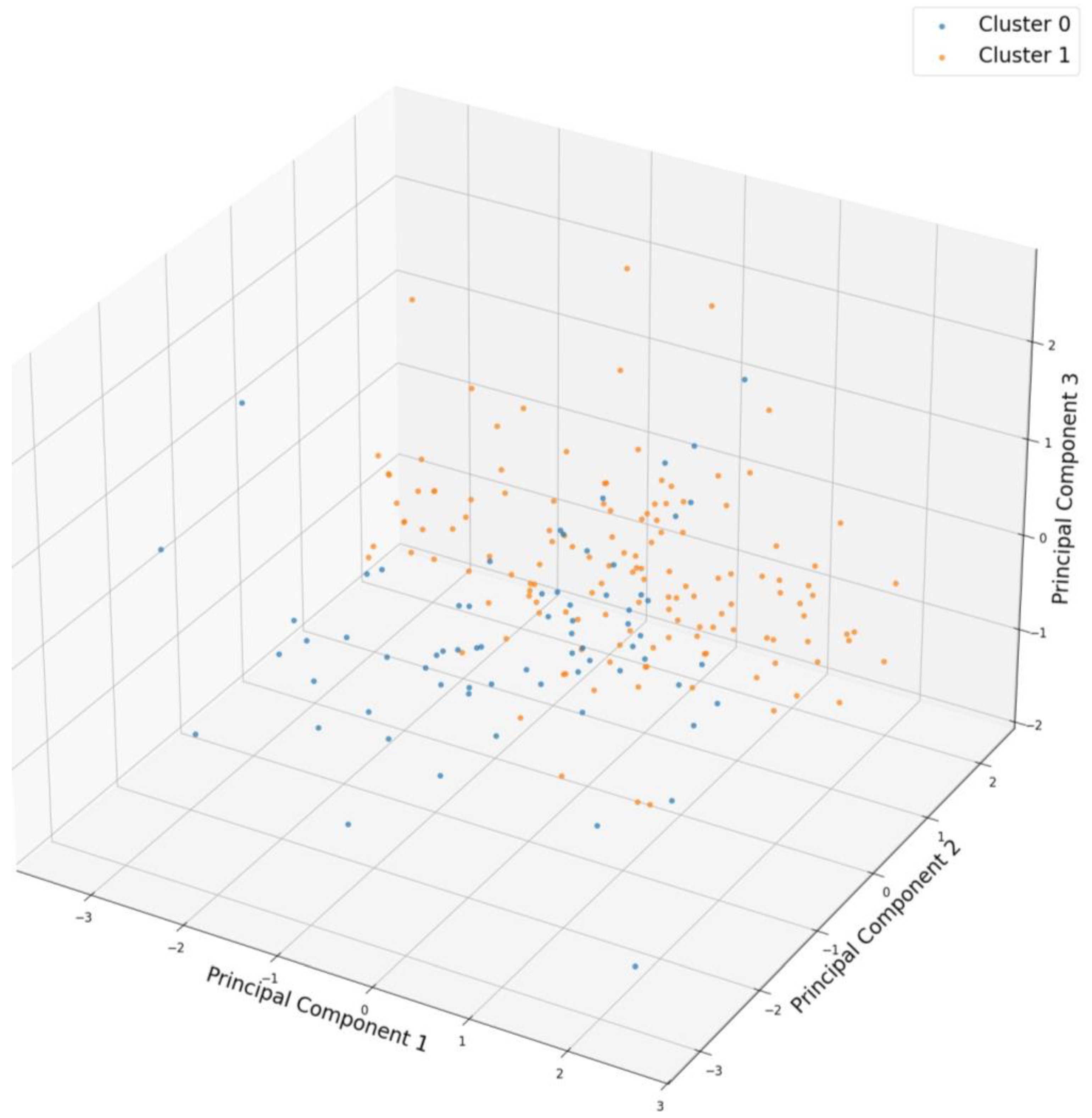
To visualize the distribution of the curves in a lower-dimensional space, Principal Component Analysis (PCA) was applied, the results of which are presented in Figure 5. In this three-dimensional representation, the blue points correspond to the series grouped in cluster 0, while the orange points represent the series in cluster 1. Partial overlap is observed between the load curves because both clusters share similar load patterns, meaning that the series within each cluster follow a common trend but are not identical. Additionally, the more dispersed points indicate greater variability within each group, reflecting small differences in the behaviors of the series and highlighting the internal diversity of each cluster. This behavior reinforces the choice of two clusters as the most appropriate and representative means of segmenting the data, ruling out the need for more clusters.

Figure 6a shows a boxplot of cross-correlation similarities, where an average close to 95% is observed, confirming the high cohesion of the curves within each cluster. On the other hand, Figure 6b presents the results of the temporal consistency index, with values above 90% seen in both clusters, validating the stability of the loading patterns over time. These indicators support the choice of the model and demonstrate that the segmentation achieved effectively captures the structure of the distribution transformer load curves.

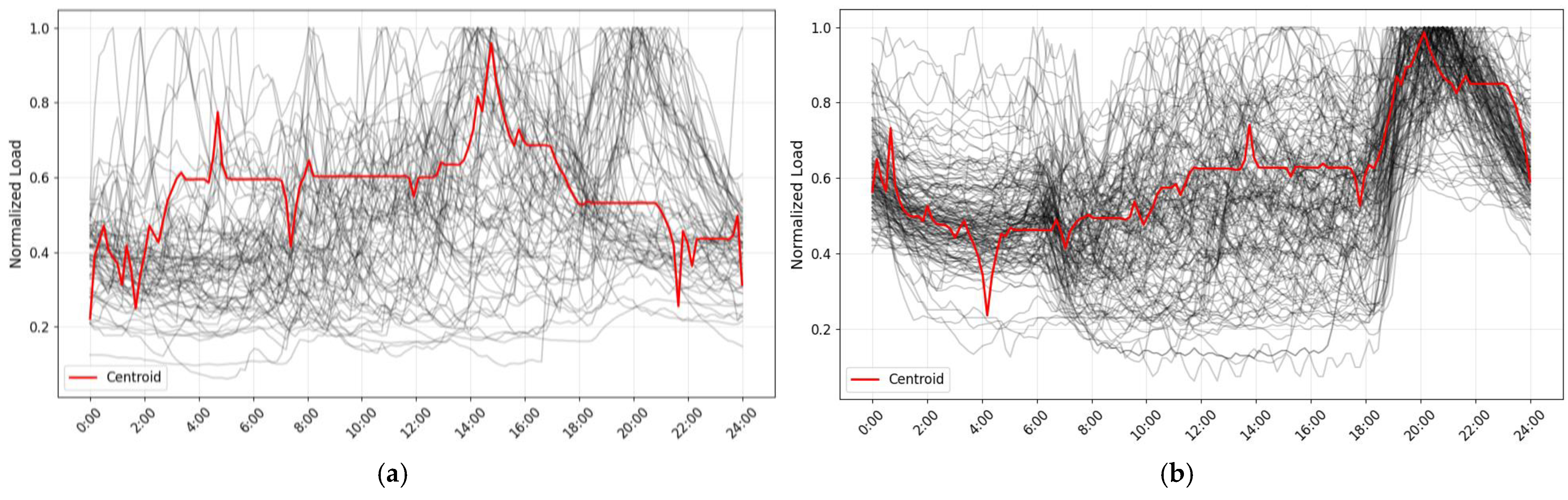
The DTW with a K-means algorithm allowed us to classify the load curves of the distribution transformers for the day of maximum demand, identifying two main types of behavior, as shown in Figure 7. In this visualization, the centroids and curves associated with each cluster are presented. However, there are peaks at the red centroids that do not allow for the adequate characterization of the load curves. To attenuate these peaks and achieve a more representative characterization of consumption patterns, the median was calculated at each point in the time series. The result of this transformation is observed in Figure 8, where median-based centroids provide a more robust view of overall load trends.

The first group of curves, shown in Figure 8a, corresponds to transformers with a higher proportion of commercial and industrial customers. These curves show an increase in load from 08:00 to 18:00, reflecting the operating hours of these types of users. Subsequently, demand decreases progressively in the evening hours. On the other hand, the second group of curves, shown in Figure 8b, characterizes predominantly residential transformers, whose consumption peaks occur after 18:00, coinciding with the switching on of public lighting and the increase in residential demand. This behavior is also evident in the reduction in consumption after 06:00, when public lighting is turned off, thus consolidating the relationship between residential consumption patterns and nighttime electricity demand.

Figure 9 shows the curves determined by DBSCAN, the gray lines are the data from the transformers and the red line is the centroid of each cluster. This algorithm does not require prior knowledge of the number of clusters; on the contrary, the algorithm automatically detects clusters thanks to its ability to identify groups of densely connected points in a dataset, which allows it to identify those curves that do not belong to any clusters as atypical or unique. As such, it is not ideal for curve characterization, which is the objective of this study. The unique curves shown in Figure 9 can be attributed to the limited number of transformer samples. If we measured a greater number of transformers with similar connected loads, it would be possible to reduce unique curves and form new groups that reflect the curves based on the different types and quantities of connected customers. This would allow for more accurate representation of electrical behavior at a global level.

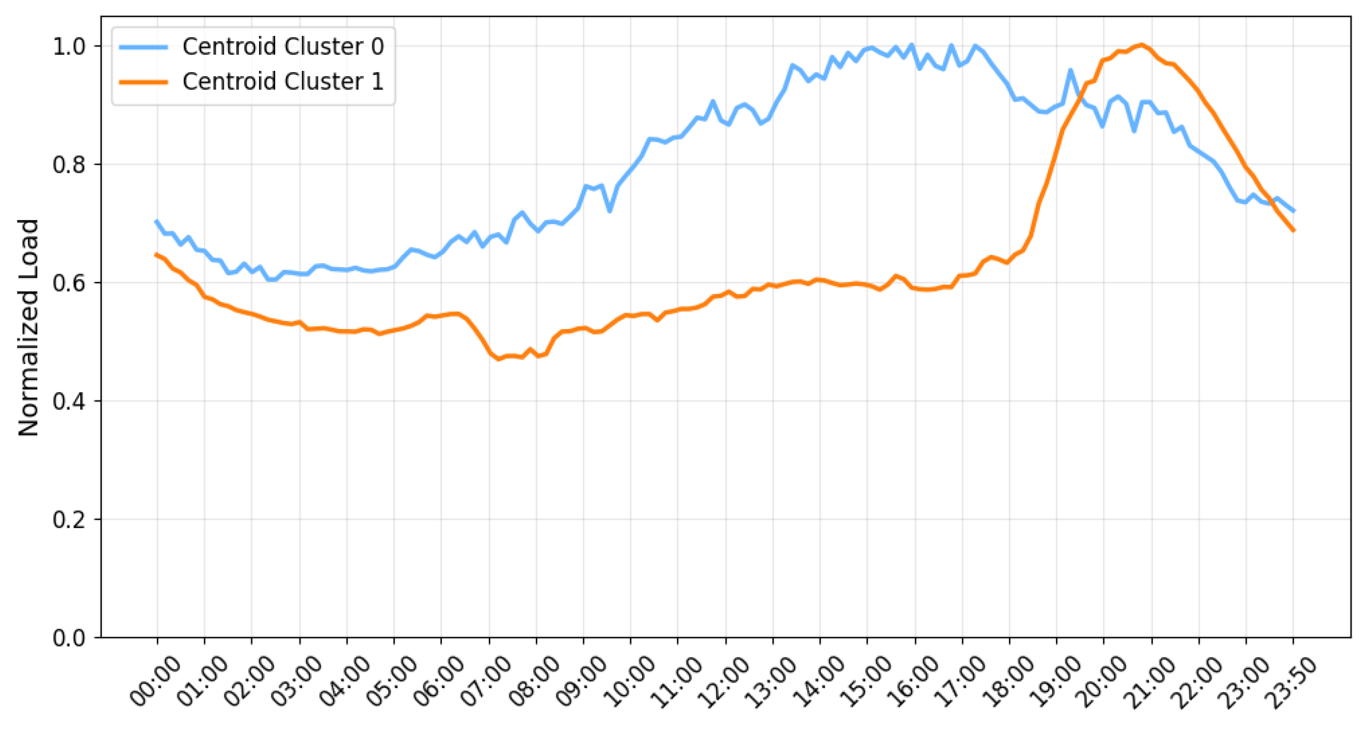
Based on the results obtained from the centroids with DTW and K-means, the curves were normalized to generate a per-unit curve, shown in Figure 10, allowing the characterization of the load curves of distribution transformers by multiplying the maximum load by each point of the characterized curve. It is important to note that the obtained load signal patterns not only facilitate the characterization of the load behavior of distribution transformers but also serve as a key tool for the management and planning of the distribution system’s operation.

The analysis of these load curves can be used to identify potential overloads or imminent failures in the equipment, facilitating the analysis of their technical condition. By integrating these load patterns into the operational planning of the distribution system, the maximum power demands in different areas can be anticipated more accurately, allowing for the more efficient adjustment of the electrical infrastructure to meet these needs.

Additionally, these patterns can contribute to dynamic load management, enabling analysis with load profiles in electrical networks to more effectively assess energy losses or the integration of distributed generation sources. These sources, which exhibit variable behavior over time, have a dynamic impact on distribution networks, with effects that are not static but rather vary depending on the different times of the day.

3.2. Transformer Curve Type Prediction Algorithm Selectrion

With the types of curves labeled on the distribution transformers using the clustering methodology, the dataset was divided, using 80% for training and 20% for testing. The objective was to develop a prediction model capable of estimating the transformer load curve as a function of the independent variables established in Table 2.

To select the most suitable algorithm, the Random Forest, Support Vector Machine (SVM), neural network, and LightGBM (Light Gradient Boosting Machine) models were evaluated. The key metrics used for the comparison are presented in

Table 8. Comparison of metrics used for selection of algorithms for transformer curve prediction.

Index	Random Forest Cluster 0/Cluster 1	Vector Support Machines Cluster 0/Cluster 1	Neural Networks Cluster 0/Cluster 1	LightGBM Cluster 0/Cluster 1
Accuracy	0.78	0.75	0.72	0.66
Recall	0.60/0.86	0.40/0.91	0.30/0.91	0.60/0.68
Precision	0.67/0.83	0.67/0.77	0.60/0.74	0.46/0.79
F1 score	0.63/0.84	0.50/0.83	0.40/0.82	0.52/0.73

. The results show that Random Forest achieved the best overall performance, standing out with an accuracy of 0.78. It also demonstrated a consistent performance across the metrics for both Cluster 0 and Cluster 1. In particular, the precision (0.67/0.83) and recall (0.60/0.86) are fairly balanced between the two clusters and show superior to the results of the other algorithms, suggesting that the model is not only capable of performing accurate classification but also maintains a good level of generalization. This means it can identify patterns and make accurate predictions about new samples not seen during training. The F1-score of 0.63/0.84 demonstrates a good balance between precision and recall, indicating that the model is able to correctly identify both common and less frequent cases, such as those in Cluster 0, without losing performance in either category. These results highlight that Random Forest has excellent generalization capabilities, adapting well to different types of data and avoiding overfitting, which is crucial for effectively predicting transformer load curves in various scenarios.

Due to its superior performance, Random Forest was selected and adjusted with the optimal parameters in

Table 9. Parameters in the Random Forest algorithm.

Parameter	Description	Value
n_estimators	Number of trees in the forest	200
min_samples_split	Minimum number of samples required to split a node into two	2
min_samples_leaf	Minimum number of samples required in a terminal leaf of a tree	1
Max_depth	Maximum depth of each tree in the forest	10
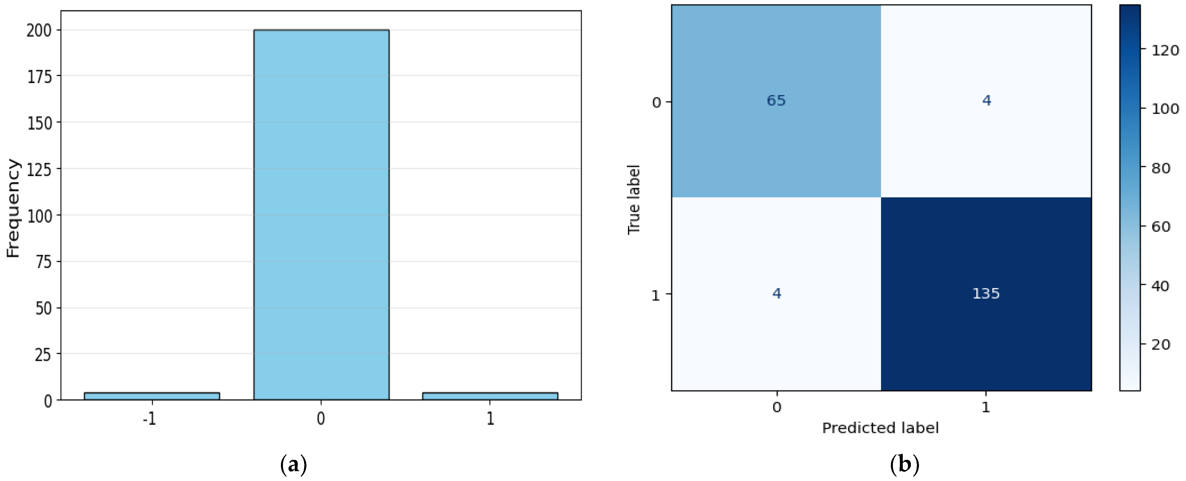
class_weight	Class weights	balanced

for the prediction of distribution transformer load curves. In Figure 11a, the difference between the actual values and the model predictions is shown, evidencing high accuracy in most cases. Additionally, Figure 11b presents the confusion matrix, where it is observed that, out of a total of 208 transformers, the model correctly predicts 200, while 8 are misclassified, yielding an accuracy of 96%.

3.3. Transformer Load Prediction Algorithm Selectrion

To determine the best algorithm for distribution transformer loadability prediction, the dataset was divided into 80% training and 20% test groups to train a distribution transformer load curve prediction model as a function of the independent variables set out in Table 3.

For the prediction of transformer loadability, four machine learning algorithms were evaluated: Random Forest, XGBoost, neural networks, and Support Vector Machine (SVR).

Table 10. Comparison of metrics for load prediction algorithms.

Index	Random Forest	XGBOOST	Neural Networks	Vector Support Machines
R2	0.82	0.85	0.77	0.90
MAE	2.91	2.90	3.86	2.28
MSE	19.48	16.65	25.24	11.20
RMSE	4.41	4.08	5.02	3.35
MAPE	36.22%	32.54%	185.28%	25.94%

presents the results obtained using the different evaluation metrics, where it is evident that the SVR model obtained the best performance, reaching an R² of 0.90, which indicates that it is capable of explaining 90% of the variability in the data. In addition, it registered the lowest Mean Absolute Error (MAE) at 2.28, the lowest Mean Squared Error (MSE) at 11.20, and an RMSE of 3.35, demonstrating greater accuracy and stability in its predictions compared to the other models. On the other hand, the neural networks algorithm shows the lowest performance with an R² of 0.77, which can be attributed to the limited amount of training data available. Although neural networks are robust models for learning complex patterns, they require large volumes of data to avoid overfitting. Without enough data, the model may lose its ability to generalize, as evidenced by the high MAPE of 185.28%.

In order to assess the impact of hyperparameters on the model results, the parameters of the models with the best scores, specifically XGBOOST and SVR, were adjusted.

Table 11. Parameters configured for sensitivity analysis.

Parameter	XGBOOST	Vector Support Machines
colsample_bytree	1	-
n_estimators	180	-
learning_rate	0.05	-
epsilon	-	0.01
C	-	1000
kernel	-	rbf

presents the modified hyperparameters, while

Table 12. Comparison of metrics for load prediction algorithms’ changing hyperparameters.

Index	XGBOOST	Vector Support Machines
R2	0.79	0.88
MAE	3.25	2.48
MSE	22.37	13.02
RMSE	4.73	3.61
MAPE	28.20%	25.68%

shows the results obtained when predicting the load of the transformers. The results indicate a decrease in model accuracy, although SVR remains the most accurate algorithm for load prediction.

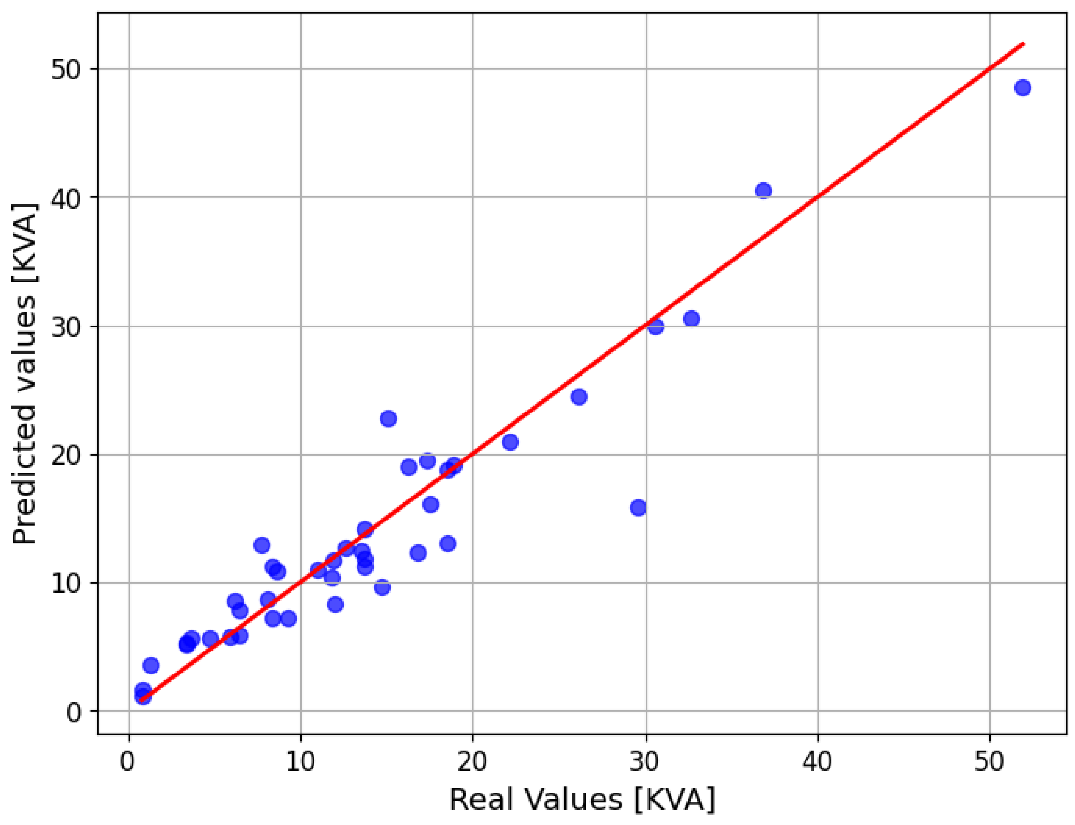
The Support Vector Machine (SVR) algorithm was selected for its superior performance in the evaluation metrics, showing better prediction capability compared to the other models tested. To optimize its performance, the parameters detailed in

Table 13. Best parameters configured in the Support Vector Machine (SVR) algorithm.

Parameter	Description	Value
C	Controls the penalty of errors.	50
epsilon	Defines the tolerable margin of error.	0.001
kernel	Function for transforming the data into a higher-dimensional space.	linear

were configured, adjusting the hyperparameter C to control the error penalty and epsilon to define the prediction tolerance. These adjustments allowed us to improve the accuracy of the estimations, ensuring a balance between bias and variance in the prediction of distribution transformer loads. In Figure 12, the graphical comparison between the real values and the power values predicted by the SVR model is presented, while Figure 13 illustrates the projection of real versus predicted loads as a function of their associated customers.

To validate model training to predict the transformer load, Figure 14a presents a residual plot where the blue points do not show any evident pattern around the red horizontal line, indicating that the model is capturing the relationships between variables correctly without systematic errors. This random behavior of the residuals suggests the good performance of the selected algorithm. On the other hand, Figure 14b shows a comparison between the distribution of real and predicted values, and a high similarity between both curves can be observed. This reinforces the validity of the model and demonstrates that the predictions made by the algorithm are consistent with the observed data, supporting its effectiveness in predicting transformer loads.

3.4. Model Evaluation

The load prediction model developed was applied to the 16,696 transformers of EEASA in operation during the year 2024. Their actual coincident power at 19:20 was 127,428.21 kVA. It is important to note that this demand only corresponds to transformers with customers metered at low voltages, and excludes those associated with private customers metered at medium voltages. This segmentation was performed with the purpose of evaluating the accuracy of the model, which predicts transformer loads based on customers, who are classified by tariff type (residential, commercial, industrial, and other) and public lighting power using data obtained from the GIS database.

The model estimated the maximum load power of each transformer and, by applying the normalized load curves found in this study, calculated the total power coincident at 19:20, obtaining a value of 129,275.67 kVA. When comparing this result with the demand registered in 2024 (127,428.21 kVA), the model was validated with an accuracy of 98.55%, which shows its high adjustment capacity and reliability in the representation of the real behavior of the demand in the distribution network.

In terms of installed capacity, the total power in transformers with customers in EEASA’s GIS database in the year 2024 amounted to 400,831 kVA, which represents an average loadability of these transformers of 31.79% (127,428.21/400,831). Applying the model to guarantee the correct distribution of infrastructure with the growth of future demand, a load increase of 40% was considered in addition to the demand projected by the model, allowing the transformers to be sized efficiently. Through this adjustment, the closest commercially available power for each transformer was determined, resulting in a 39.27% reduction in installed power, from 400,831 kVA to 243,437.50 kVA, with a new average loadability of 52.35%.

In Figure 15, the power distribution of real transformers (blue) compared to the suggested transformers (orange) is shown. A significant increase is observed in transformers of 5 kVA and 15 kVA, which indicates a reduction in the installation of equipment of 10, 25, and 37.5 kVA, as well as equipment with higher capacities. This resizing allows for greater efficiency in the use of the electrical infrastructure, optimizing the operation without compromising the reliability of the system.

3.5. Analysis and Discussions

This study highlights how the use of advanced data science and machine learning techniques can significantly improve the characterization and prediction of distribution transformer load curves. In the initial phase of the analysis, the segmentation of time series using clustering algorithms allowed the identification of distinct patterns of power consumption. The comparison of internal validation metrics shows that the DTW method with K-means offers a superior clustering structure, standing out for its low centroid representation error (0.6177) and high Temporal Consistency (0.9642), which reflects adequate coherence in the temporal behavior of the data. In contrast, although DBSCAN showed good performance in detecting single curves, its low compactness and high Davies–Bouldin index (1.0736) indicate that it is not the most suitable method for the generalized segmentation of load curves. Furthermore, the analysis of other metrics, such as the Silhouette Index (0.355) and the Calinski–Harabasz Index (179.4344), for DTW with K-means reinforces the ability of this approach to generate more compact and well-defined groupings. These results underscore the importance of complementing quantitative metrics with the expert validation of the electrical domain, which allows for the accurate interpretation of the relevance of each clustering in electrical infrastructure planning.

From the point of view of predictive modeling, the results highlight that algorithm selection depends on the nature of the problem. In the classification of load curves, Random Forest showed the best performance, reaching an accuracy of 78%, and maintained a good balance between recall and accuracy, making it a suitable choice for this task. Regarding the prediction of the power demanded by the transformers, Support Vector Machine (SVR) proved to be superior, with an R² of 0.90, the lowest MAE (2.28), and the lowest RMSE (3.35). These results are consistent with previous studies, such as that of Ref. [22], which used SVR to predict the energy consumption of electric boilers with an R² of 0.84. In contrast, other approaches, such as Multilayer Perceptron (MLP) artificial neural networks (ANNs), did not perform well, suggesting that these techniques have limitations in this context. In research such as Ref. [12], overfitting problems were found in LSTM models, which reinforces the advantage of simpler and more efficient models such as SVR. In turn, the transformer model, although promising, showed considerable variability in its performance depending on the specific transformer, indicating that this type of model may require a more adaptive approach in dynamic scenarios. Compared to the hybrid approach proposed in Ref. [17], which combined GRUs and TCNs, the SVR algorithm used in this study achieved comparable results, but with a more simplified model.

On the other hand, the neural networks applied in this study did not perform well, especially in terms of MAPE (185.28%) and R² (0.77), suggesting that this model does not adequately fit the data in this task. In summary, SVR stands out as the most robust model; these findings reinforce the idea that, in regression problems applied to electrical infrastructure, models based on convex optimization techniques, such as SVR, can be more effective than deep learning approaches, which often require finer hyperparameter tuning to achieve stability.

Finally, the application of the prediction model to EEASA’s 16,696 transformers allowed us to estimate a projected coincident power of 129,275.67 kVA, validating the model with an accuracy of 98.55%. This suggests that the model has high reliability and can be used with confidence for decision making. In addition, the optimization in transformer allocation resulted in a 39.27% reduction in installed power, from 400,831 kVA to 243,437.50 kVA, with an improvement in average loadability, which increased from 31.79% to 52.35%. These results underscore the positive impact of machine learning on energy management, allowing for the more efficient sizing of electrical infrastructure and more sustainable planning. However, although the results of the study are favorable, it is recommended to include a larger number of transformer samples to further improve the training of the model and cover all possible combinations of consumers connected to this equipment.

4. Conclusions

This study addresses a critical challenge facing electric utilities, the optimization of the sizing of distribution transformers, which is key in improving operational efficiency and reducing costs. Through the analysis of historical load data from transformers, an approach based on machine learning techniques is proposed to characterize load curves and predict the maximum load of transformers. The innovation of our work lies in the integration of clustering techniques and predictive models, which allows us to classify the load curves and precisely predict the maximum load of transformers based on variables such as the type and quantity of connected customers, geographic location, and other relevant factors.

This study highlights the importance of applying advanced data science techniques to demand optimization and load curve characterization in distribution transformers. The implementation of unsupervised algorithms such as K-shape, DBSCAN, and DTW with K-means, along with internal validation metrics such as Silhouette, Davies–Bouldin, and Calinski–Harabasz, allowed for evaluating the segmentation quality. However, it was observed that these metrics, although useful, are not sufficient on their own, requiring the intervention of experts in the electrical domain to validate the results.

In addition, predictive models, based on supervised algorithms such as Random Forest, LightGBM, Support Vector Machines, and neural networks, were employed. This allowed us to compare their ability to classify curve types and predict transformer loading. It was found that Random Forest achieved a good balance between accuracy and recall, facilitating more equitable prediction between categories. On the other hand, the SVR model stood out in regression, reaching an R² of 0.90 and the lowest absolute error, positioning it as the best option for predicting transformer loadability. It provides a balance between accuracy, stability, and generalization capacity—key factors for decision making in the planning and optimization of electrical infrastructure. However, the results highlight that the choice of model should be based on overall accuracy and its ability to handle unbalanced data distributions and outliers.

The results obtained show that this approach optimizes the utilization factor of transformers, reducing the installed capacity without compromising operational efficiency. This not only improves grid planning and operation but also contributes significantly to the sustainability of the system through the more efficient management of energy resources. Moreover, the proposed methodology provides a dynamic and more accurate way to size transformers, considering the variability of electrical demand throughout the day—an aspect that has been scarcely explored in the existing literature. This key innovation allows electric utilities to optimize infrastructure in a way that is more closely aligned with real consumption needs and demand variability.

In future work, we plan to explore the inclusion of deep learning models, such as Long Short-Term Memory (LSTM) networks, to further investigate their potential in transformer load prediction. Additionally, we aim to explore dimensionality reduction techniques like Principal Component Analysis (PCA) and t-Distributed Stochastic Neighbor Embedding (t-SNE) to enhance cluster analysis for load curve characterization. Furthermore, acquiring a larger dataset of load records would enable the more precise modeling of electrical consumption patterns, which would ultimately improve the accuracy and generalization of the prediction models.

References

1. Di Lorenzo, G.; Yadiyal, K. Sustainable power system planning for India: Insights from a modelling and simulation perspective. Energy Nexus 2024, 13, 100261. [Google Scholar] [CrossRef]
2. Hussain, F.; Hasanuzzaman, M.; Rahim, N.A. Multivariate machine learning algorithms for energy demand forecasting and load behavior analysis. Energy Convers. Manag. X 2025, 26, 100903. [Google Scholar] [CrossRef]
3. Giannelos, S.; Zhang, T.; Pudjianto, D.; Konstantelos, I.; Strbac, G. Investments in Electricity Distribution Grids: Strategic versus Incremental Planning. Energies 2024, 17, 2724. [Google Scholar] [CrossRef]
4. Junior, L.C.D.S.; Tabora, J.M.; Reis, J.; Andrade, V.; Carvalho, C.; Manito, A.; Tostes, M.; Matos, E.; Bezerral, U. Demand-Side Management Optimization Using Genetic Algorithms: A Case Study. Energies 2024, 17, 1463. [Google Scholar] [CrossRef]
5. Dai, Z.; Shi, K.; Zhu, Y.; Zhang, X.; Luo, Y. Intelligent Prediction of Transformer Loss for Low Voltage Recovery in Distribution Network with Unbalanced Load. Energies 2023, 16, 4432. [Google Scholar] [CrossRef]
6. León-Martínez, V.; Peñalvo-López, E.; Andrada-Monrós, C.; Sáiz-Jiménez, J.Á. Load Losses and Short-Circuit Resistances of Distribution Transformers According to IEEE Standard C57.110. Inventions 2023, 8, 154. [Google Scholar] [CrossRef]
7. Wang, X.; Guo, Q.; Tu, C.; Li, J.; Xiao, F.; Wan, D. A two-stage optimal strategy for flexible interconnection distribution network considering the loss characteristic of key equipment. Int. J. Electr. Power Energy Syst. 2023, 152, 109232. [Google Scholar] [CrossRef]
8. Oliyide, R.O.; Cipcigan, L.M. Adaptive thermal model for loading of transformers in low carbon electricity distribution networks. Sci. Afr. 2023, 20, e01683. [Google Scholar] [CrossRef]
9. Rafati, A.; Mirshekali, H.; Shaker, H.R. Overload Alarm Prediction in Power Distribution Transformers. Smart Grids Sustain. Energy 2024, 9, 1–14. [Google Scholar] [CrossRef]
10. Hung, Y.-C.; Liu, D.-R. Power Peak Load Forecasting Based on Deep Time Series Analysis Method. IEICE Trans. Inf. Syst. 2024, 107, 845–856. [Google Scholar] [CrossRef]
11. Ashetehe, A.A.; Shewarega, F.; Gessesse, B.B.; Biru, G.; Lakeou, S. A stochastic approach to determine the energy consumption and synthetic load profiles of different customer types of rural communities. Sci. Afr. 2024, 24, e02172. [Google Scholar] [CrossRef]
12. Schröder, K.; Farias, G.; Dormido-Canto, S.; Fabregas, E. Comparative Analysis of Deep Learning Methods for Fault Avoidance and Predicting Demand in Electrical Distribution. Energies 2024, 17, 2709. [Google Scholar] [CrossRef]
13. Hajiaghapour-Moghimi, M.; Azimi-Hosseini, K.; Hajipour, E.; Vakilian, M. Residential Load Clustering Contribution to Accurate Distribution Transformer Sizing. In Proceedings of the 34th International Power System Conference, PSC 2019, Tehran, Iran, 9–11 December 2019; pp. 313–319. [Google Scholar] [CrossRef]
14. Neagu, B.; Grigoras, G.; Scarlatache, F.; Schreiner, C.; Ciobanu, R. Patterns discovery of load curves characteristics using clustering based data mining. In Proceedings of the 2017 11th IEEE International Conference on Compatibility, Power Electronics and Power Engineering, CPE-POWERENG 2017, Cadiz, Spain, 4–6 April 2017; pp. 83–87. [Google Scholar] [CrossRef]
15. Yuan, S.; Zhang, X.; Geng, J.; Wan, D. Research on load curve clustering of distribution transformer based on wavelet transform and big data processing. In Proceedings of the 2017 IEEE 2nd Information Technology, Networking, Electronic and Automation Control Conference, ITNEC 2017, Chengdu, China, 15–17 December 2017; pp. 348–351. [Google Scholar] [CrossRef]
16. Xia, W.; Huang, H.; Duque, E.M.S.; Hou, S.; Palensky, P.; Vergara, P.P. Comparative assessment of generative models for transformer- and consumer-level load profiles generation. Sustain. Energy Grids Netw. 2024, 38, 101338. [Google Scholar] [CrossRef]
17. Wen, X.; Liao, J.; Niu, Q.; Shen, N.; Bao, Y. Deep learning-driven hybrid model for short-term load forecasting and smart grid information management. Sci. Rep. 2024, 14, 1–16. [Google Scholar] [CrossRef]
18. Patil, P.D.; Patil, R.; Ahire, P.; Bharati, R.; Dongre, Y. An adaptive methodology based on predictive deep learning and context aware clustering for electricity power usage mining and optimization at different granularity levels. E-Prime Adv. Electr. Eng. Electron. Energy 2024, 8, 100628. [Google Scholar] [CrossRef]
19. Syed, D.; Abu-Rub, H.; Ghrayeb, A.; Refaat, S.S.; Houchati, M.; Bouhali, O.; Banales, S. Deep Learning-Based Short-Term Load Forecasting Approach in Smart Grid with Clustering and Consumption Pattern Recognition. IEEE Access 2021, 9, 54992–55008. [Google Scholar] [CrossRef]
20. MacMackin, N.; Miller, L.; Carriveau, R. Investigating distribution systems impacts with clustered technology penetration and customer load patterns. Int. J. Electr. Power Energy Syst. 2021, 128, 106758. [Google Scholar] [CrossRef]
21. Gunkel, P.A.; Jacobsen, H.K.; Bergaentzlé, C.-M.; Scheller, F.; Andersen, F.M. Variability in electricity consumption by category of consumer: The impact on electricity load profiles. Int. J. Electr. Power Energy Syst. 2023, 147, 108852. [Google Scholar] [CrossRef]
22. Kachalla, I.A.; Ghiaus, C.; Baseer, M. Comparative analysis of machine learning models for prediction and forecasting of electric water boilers energy consumption. Appl. Therm. Eng. 2025, 267, 125799. [Google Scholar] [CrossRef]
23. Wang, W.; Shimakawa, H.; Jie, B.; Sato, M.; Kumada, A. BE-LSTM: An LSTM-based framework for feature selection and building electricity consumption prediction on small datasets. J. Build. Eng. 2025, 102, 111910. [Google Scholar] [CrossRef]
24. Shwetha, B.N.; Kumar, H.K.S. Prediction of Electricity Consumption in Residential Areas using Temporal Fusion Transformer and Convolutional Neural Network. J. Mach. Comput. 2025, 5, 209–219. [Google Scholar] [CrossRef]
25. Pyzdek, T. Pareto Analysis. In Management for Professionals; Springer: Berlin/Heidelberg, Germany, 2021; Part F458. [Google Scholar] [CrossRef]
26. Stojčić, M.; Banjanin, M.K.; Vasiljević, M.; Nedić, D.; Stjepanović, A.; Danilović, D.; Puzić, G. Predictive Modeling of Delay in an LTE Network by Optimizing the Number of Predictors Using Dimensionality Reduction Techniques. Appl. Sci. 2023, 13, 8511. [Google Scholar] [CrossRef]
27. Dang-Ha, T.-H.; Olsson, R.; Wang, H. Clustering Methods for Electricity Consumers: An Empirical Study in Hvaler-Norway. arXiv 2017, arXiv:1703.02502. [Google Scholar]
28. Toussaint, W.; Moodley, D. Clustering residential electricity consumption data to create archetypes that capture household behaviour in south Africa. South Afr. Comput. J. 2020, 32, 1–34. [Google Scholar] [CrossRef]
Figure 1. Scheme for sizing and characterization of load curves of distribution transformers.
Energies 18 01832 g001
Figure 2. Frequency of transformers vs. Power KVA per customer: (a) total transformers; (b) valid transformers without extreme values.
Energies 18 01832 g002
Figure 3. Transformer hourly real loads [KVA].
Energies 18 01832 g003
Figure 4. Methods used to determine the number of clusters of DTW with K-means: (a) Elbow Method; (b) Silhouette Scoring Method.
Energies 18 01832 g004
Figure 5. Principal Component Analysis of DTW with K-means.
Energies 18 01832 g005
Figure 6. The cohesion or similarity in the shape of the load curves and the stability or temporal consistency of the time series over time using DTW with K-means: (a) boxplot of the cross-correlation similarity index of the load curve clusters; (b) temporal consistency index of the load curve clusters.
Energies 18 01832 g006
Figure 7. Load curves classified in each cluster, with centroids in red—DTW with K-means: (a) load curve cluster 0; (b) load curve cluster 1.
Energies 18 01832 g007
Figure 8. Characteristic load curves applying the median—DTW with K-means: (a) centroid cluster 0; (b) centroid cluster 1.
Energies 18 01832 g008
Figure 9. Load curve centroids—DBSCAN.
Energies 18 01832 g009
Figure 10. Normalized characteristic curves of transformers.
Energies 18 01832 g010
Figure 11. Shows the precision in predicting the type of curve: (a) difference in actual and predicted values of transformer curve type [Cluster DTW_KMeans—Cluster Predicted]; (b) donfusion matrix of transformer curve type predictions.
Energies 18 01832 g011
Figure 12. Difference between real and predicted values of transformer loading.
Energies 18 01832 g012
Figure 13. Scatter plot of real and predicted values of transformer loading.
Energies 18 01832 g013
Figure 14. The validation of the transformer load prediction SVR Model: (a) residual analysis; (b) the comparison of real and predicted value distributions.
Energies 18 01832 g014
Figure 15. Distribution of current and suggested transformer powers at EEASA.
Energies 18 01832 g015