
Lumped-Parameter Models Comparison for Natural Ventilation Analyses in Buildings at Urban Scale


Abstract
1. Introduction
2. Objective of the Work
3. Methods
3.1. Analyzed Buildings
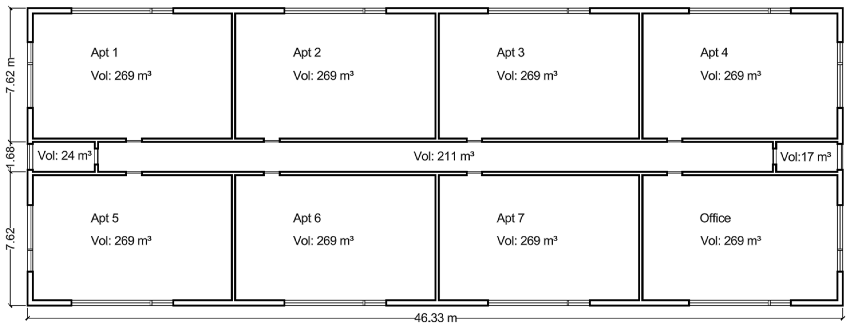
3.1.1. Midrise Prototype Building
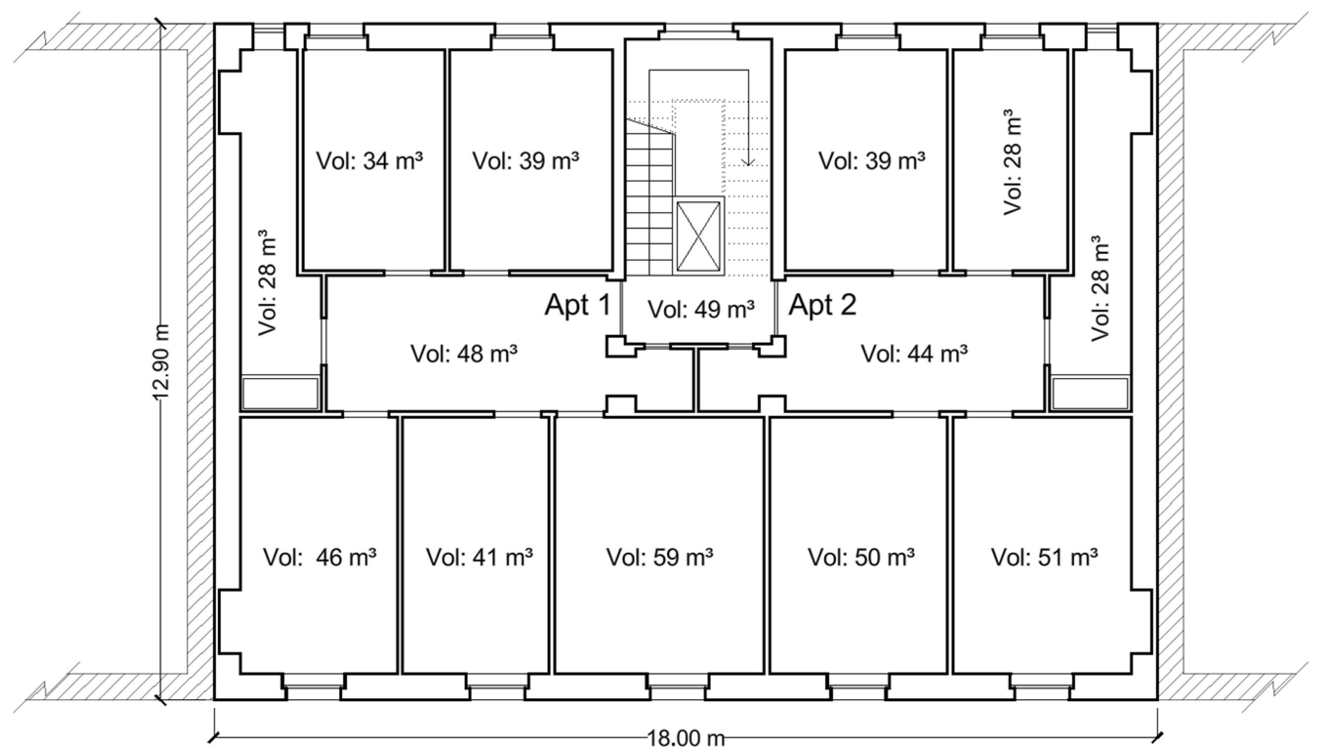
3.1.2. Turin Building
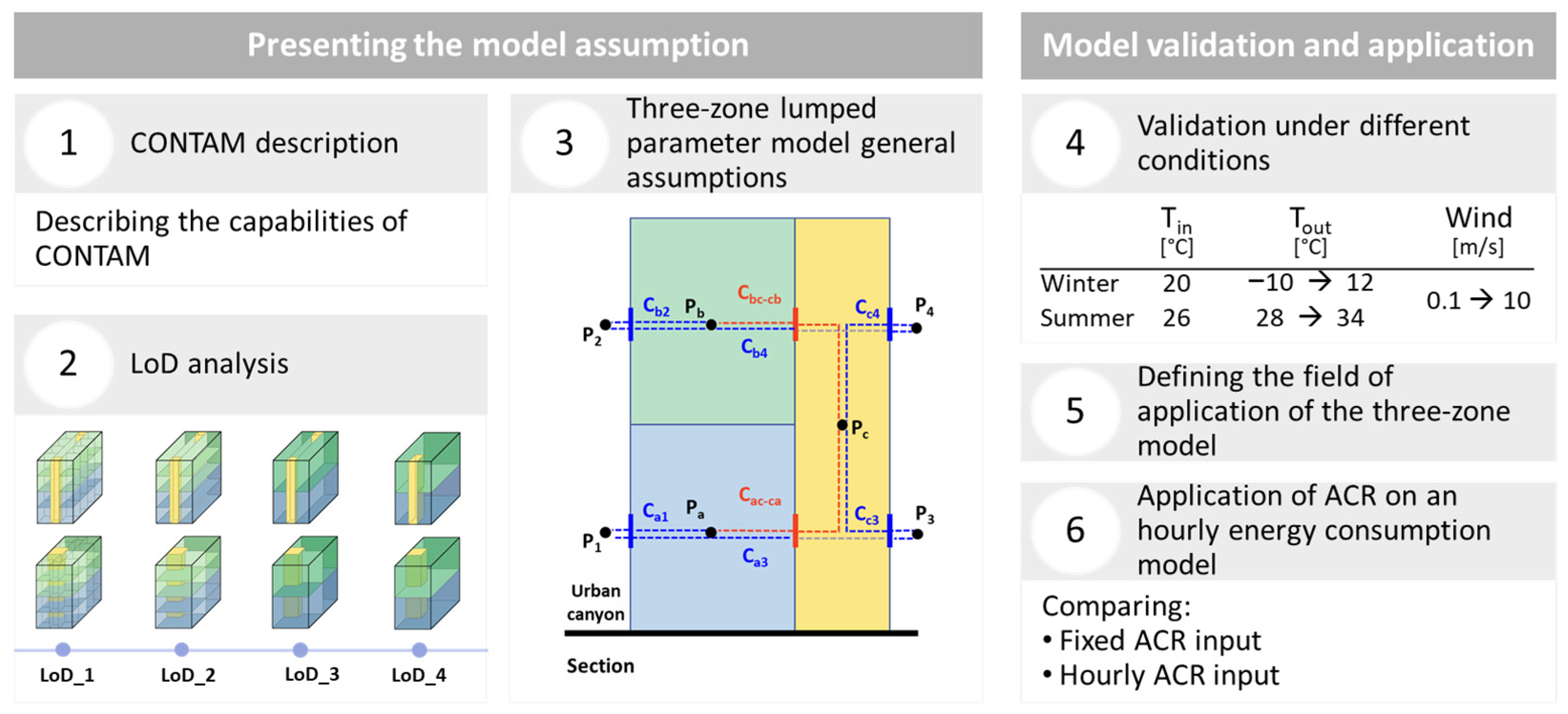
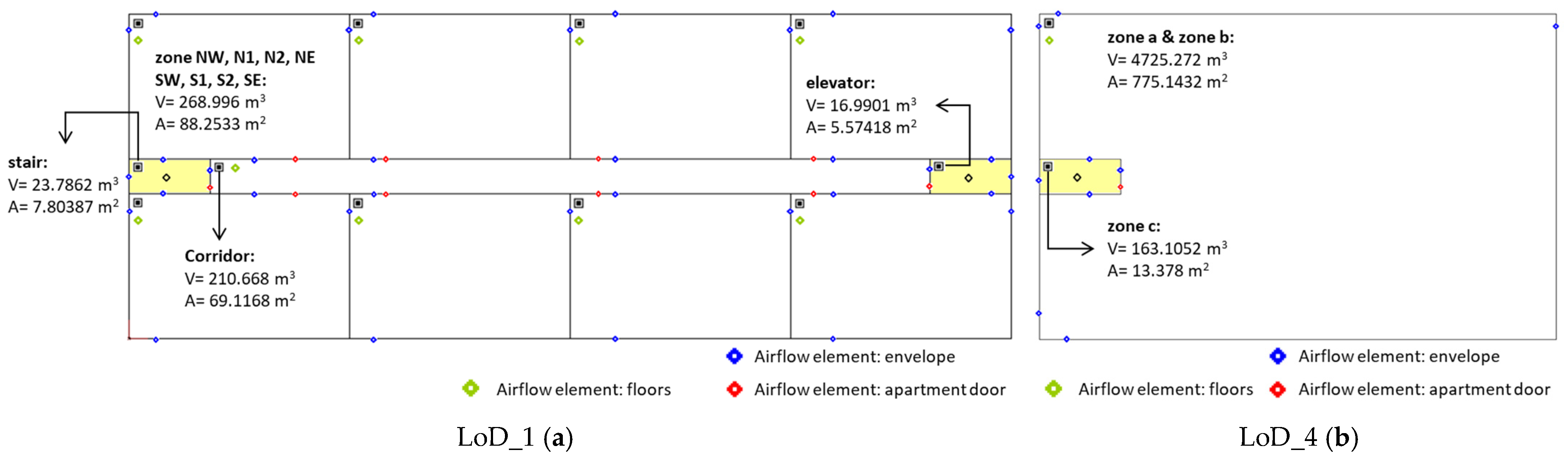
3.2. Level of Detail (LoD) Analysis
3.2.1. CONTAM
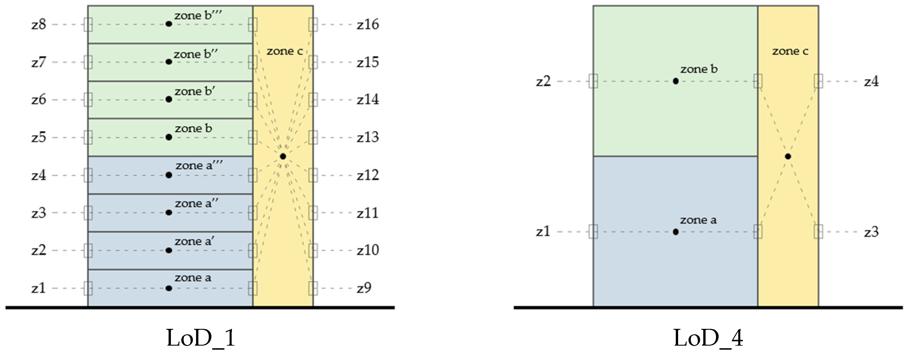
3.2.2. LoD Steps
3.2.3. LoD Models in CONTAM
- Qr is the predicted airflow rate at ΔPr (from pressurization test data) [L/s/m2]
- Cd is the discharge coefficient [-], used here as 1
- AL is the leakage area [cm2/m2]
- is the air density [kg/m3]
- ΔPr is the reference pressure difference (from pressurization test data) [Pa]
- n is the flow exponent [-], used here as 0.65
- ΔP is the pressure difference, used here as 4 Pa.
- Cd,opening is the discharge coefficient of the opening [-], used here as 0.65
- Aleakage is the leakage area of the opening [m2]
- is the air density [kg/m3]
- AL is the leakage area [cm2/m2], used here as 12 cm2/m2
- Aopening is the opening area of the airflow element [m2], used here as 1.98 m2.
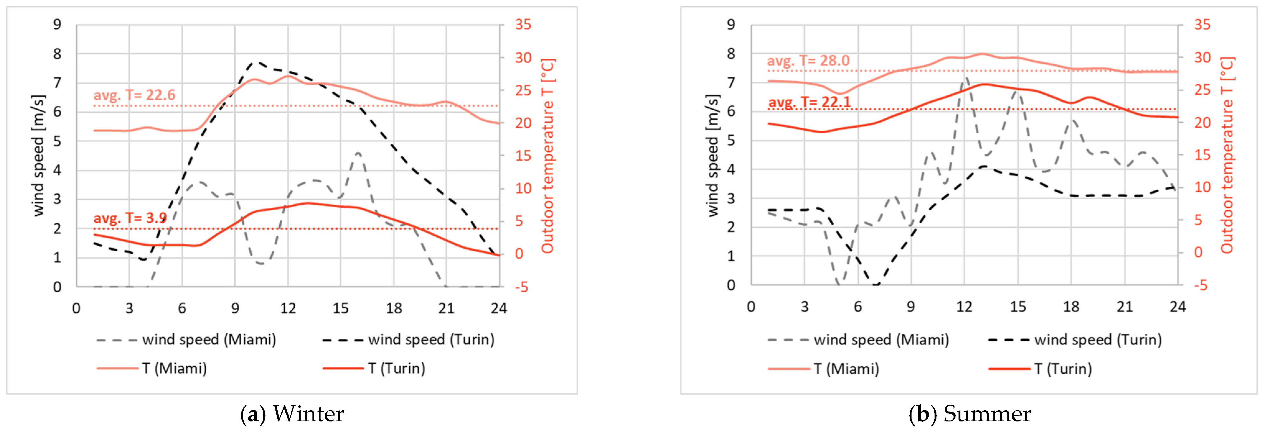
3.2.4. LoD Indoor Temperature and Weather Data
3.3. Three-Zone Lumped-Parameter Model
3.3.1. General Aim
3.3.2. Corrected Wind Speed
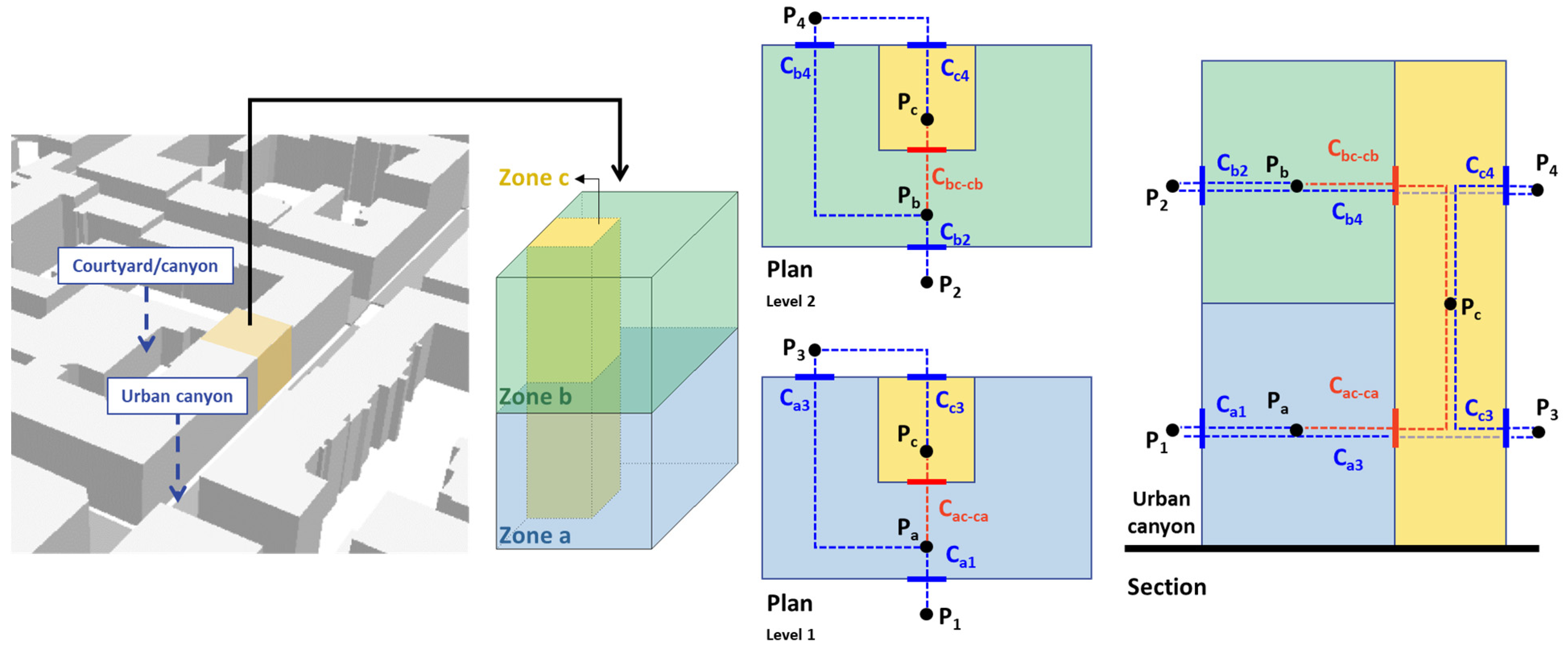
3.3.3. Three-Zone Building Simplification
Geometrical Simplification
Physical Assumptions
- C is the flow coefficient [kg·s−1·Pa−n]
- is the airflow rate [kg/s]
- ΔP is the total pressure difference [Pa].
Validation with CONTAM
4. Results
- is the actual value
- is the predicted value
- is the total number of observations.
4.1. Level of Detail (LoD) Analysis Using CONTAM
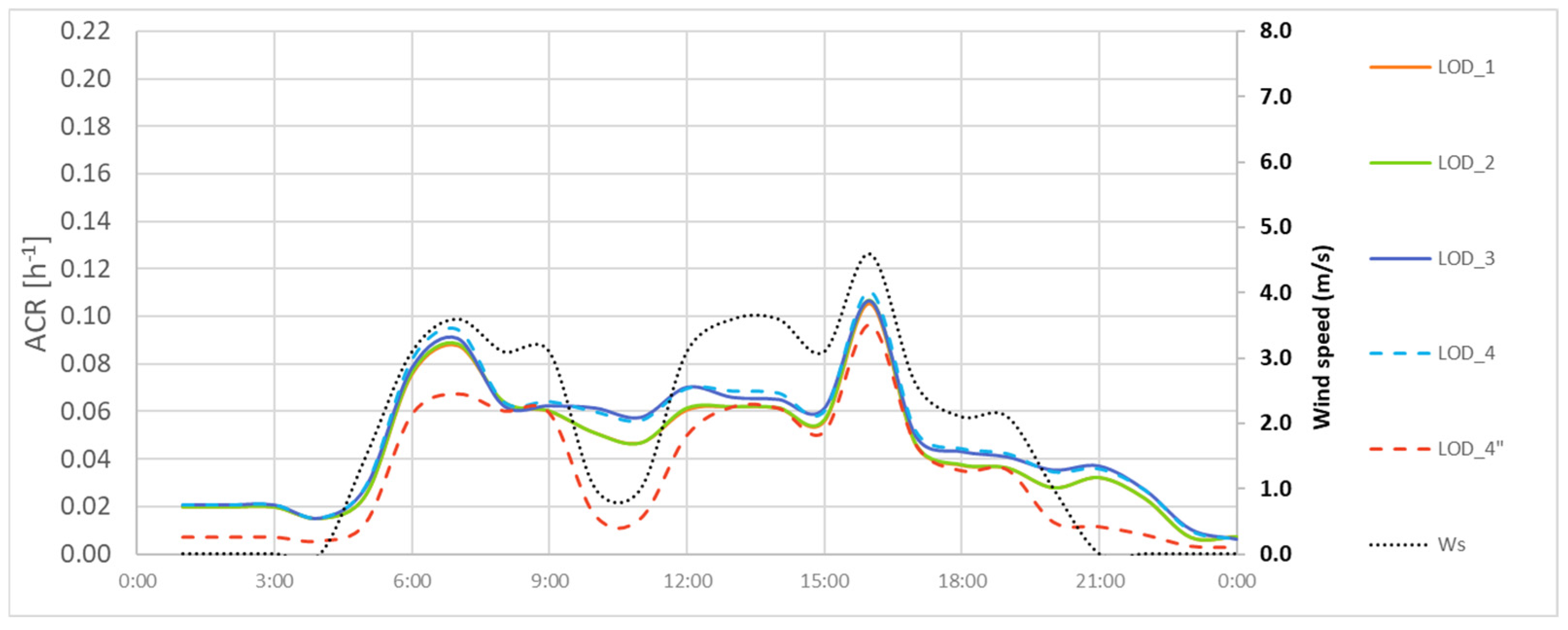
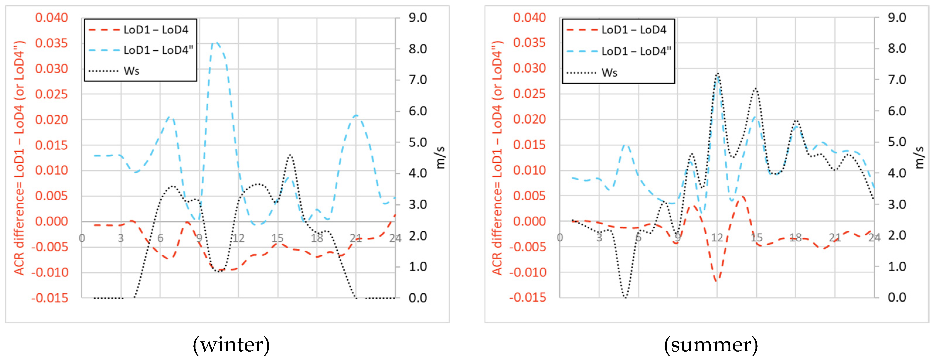
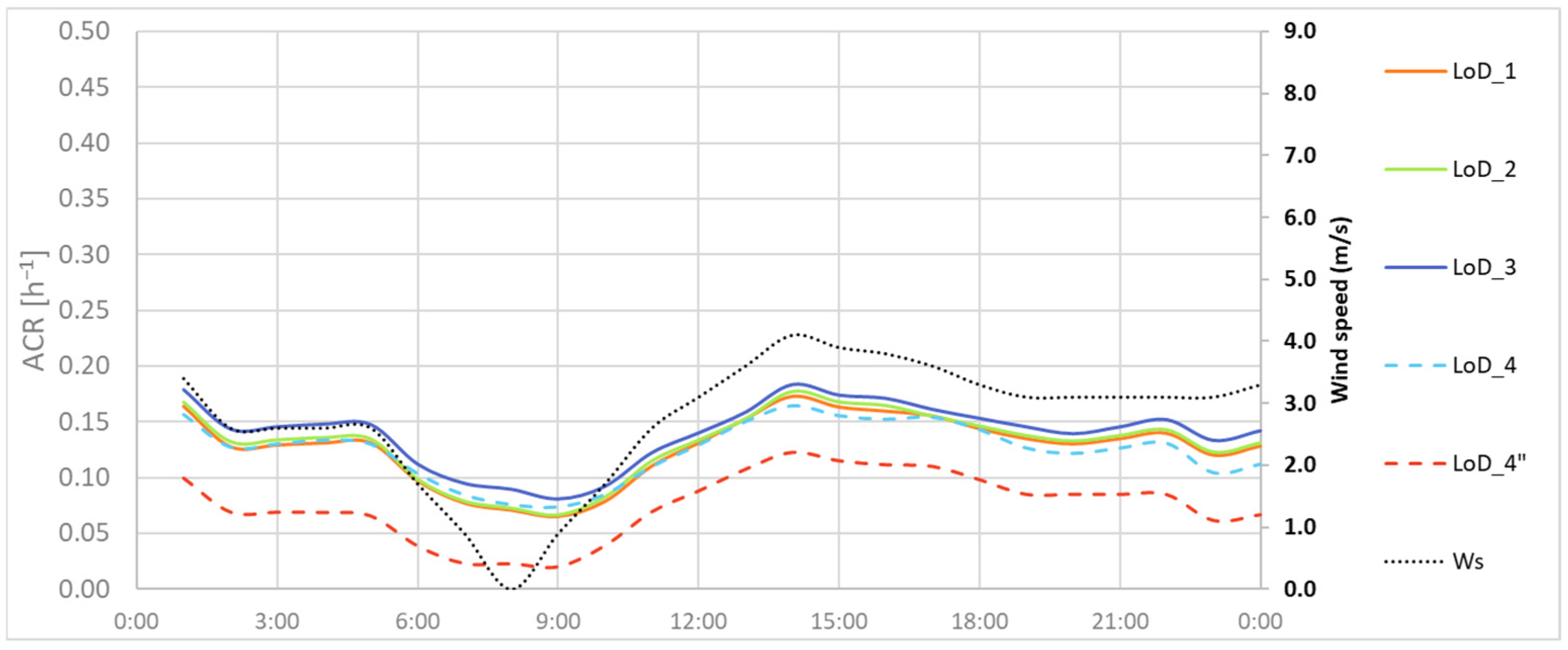
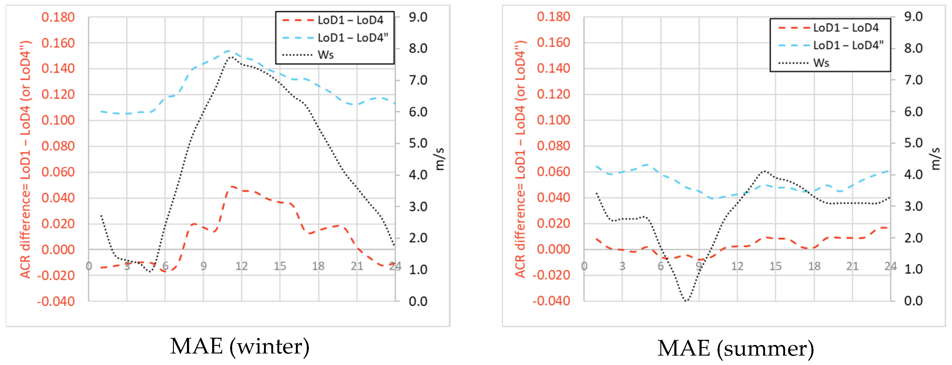
4.1.1. Midrise Prototype Building Results
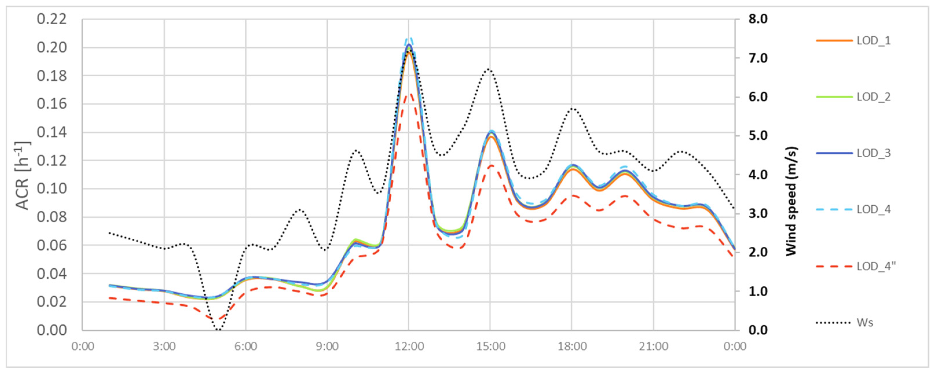
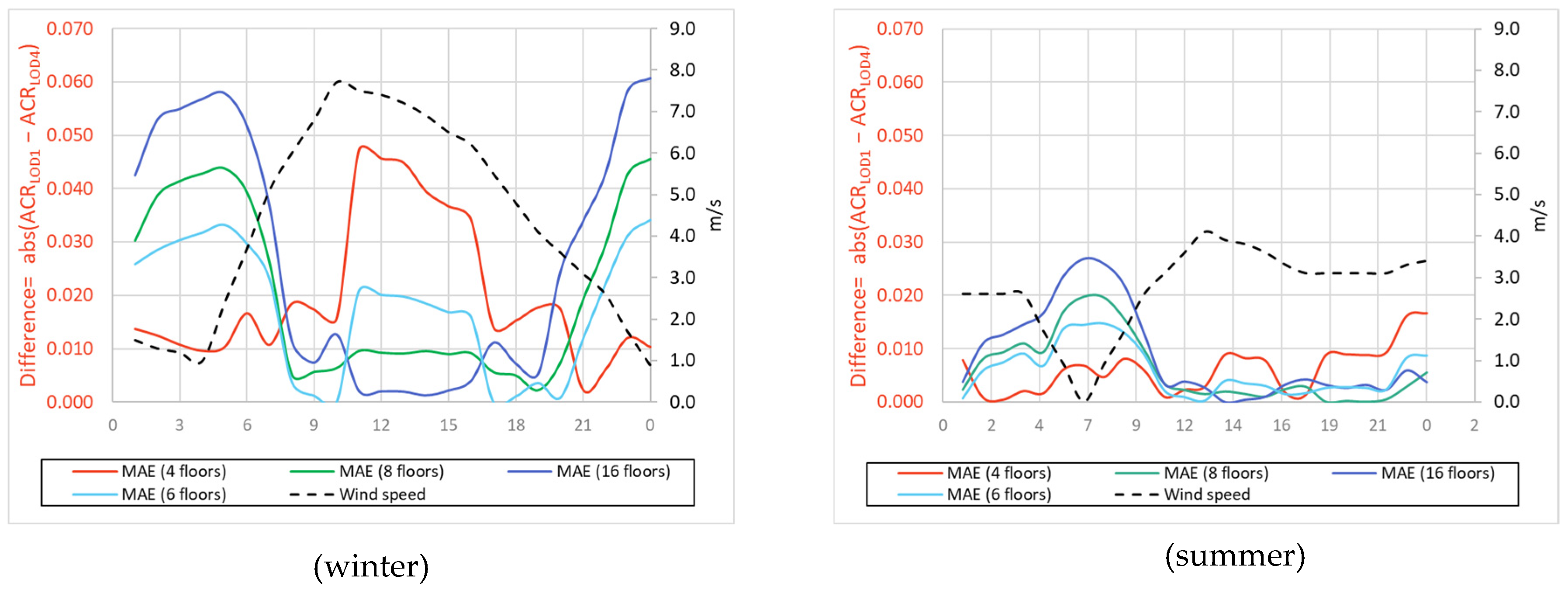
4.1.2. Turin Building Results
4.1.3. Summary
4.2. Three-Zone Lumped-Parameter Model Validation with CONTAM
4.3. Field of Application Analysis
4.4. Example Application: Energy Consumption for Space Heating
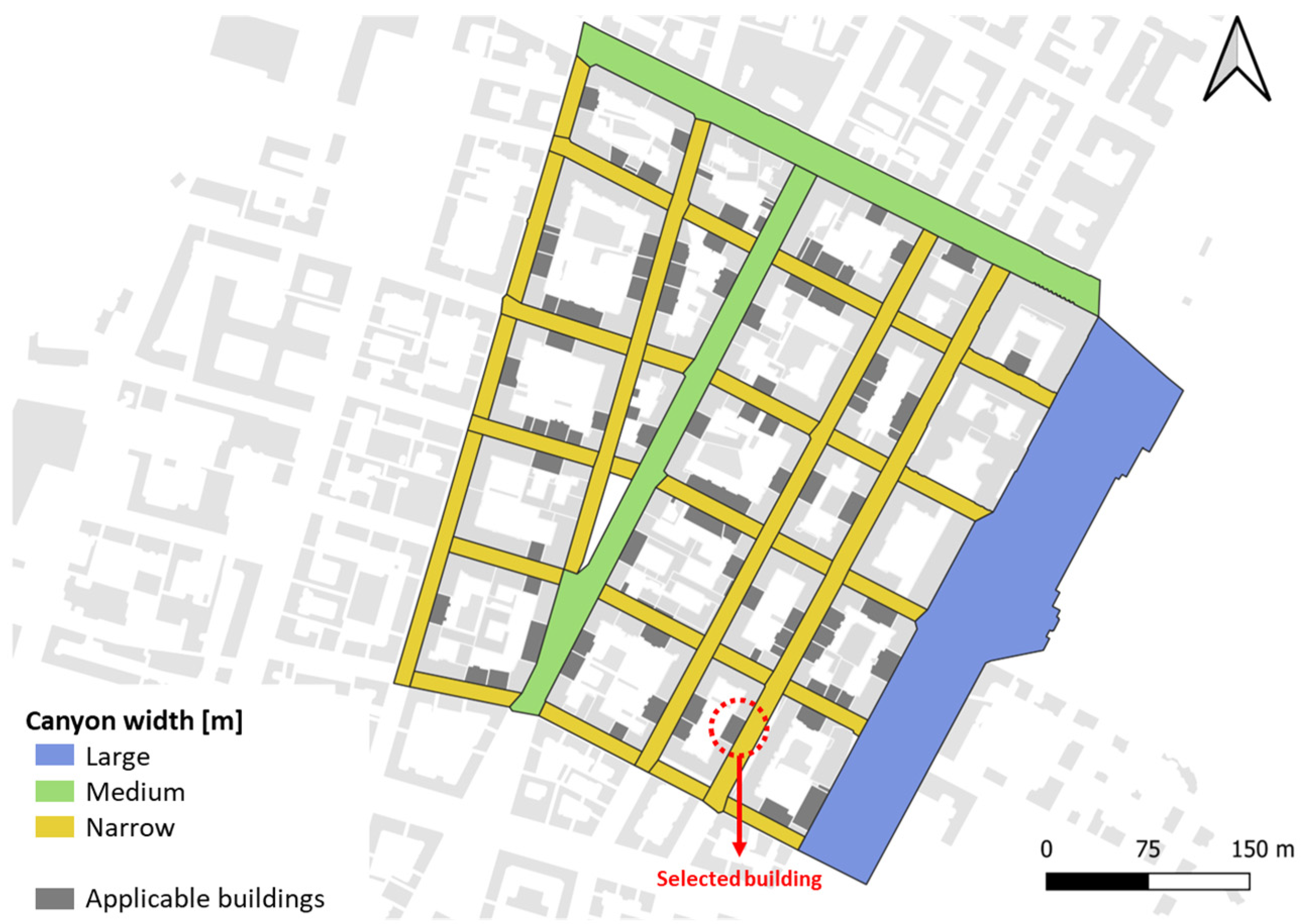
4.4.1. Selected Building
- Building characteristics including the construction period (i.e., 1919–1945), the associated ACR value, and thermal properties, such as thermal capacity (Ct) and thermal transmittance (U) for both opaque (walls, roof, ground) and transparent (glazing) building envelopes, the window-to-wall ratio (WWR), heating system efficiency (η). Reference data are provided in Table 5, with the selected building’s construction period highlighted.
- Local weather data includes hourly outdoor air temperature, humidity, pressure, solar radiation, and sun altitude, recorded by the weather station of Politecnico di Torino [38] for the period from May 2022 to April 2023, in which the hourly consumption data are available.
- Heating schedule, which details the building’s occupancy patterns and the operation of the centralized heating system. In the analyzed scenarios, the system operates according to national and local regulations, with the internal air temperature of 19 °C during the day from 6 am to 9 pm with two interruptions at 9 am and 2 pm.
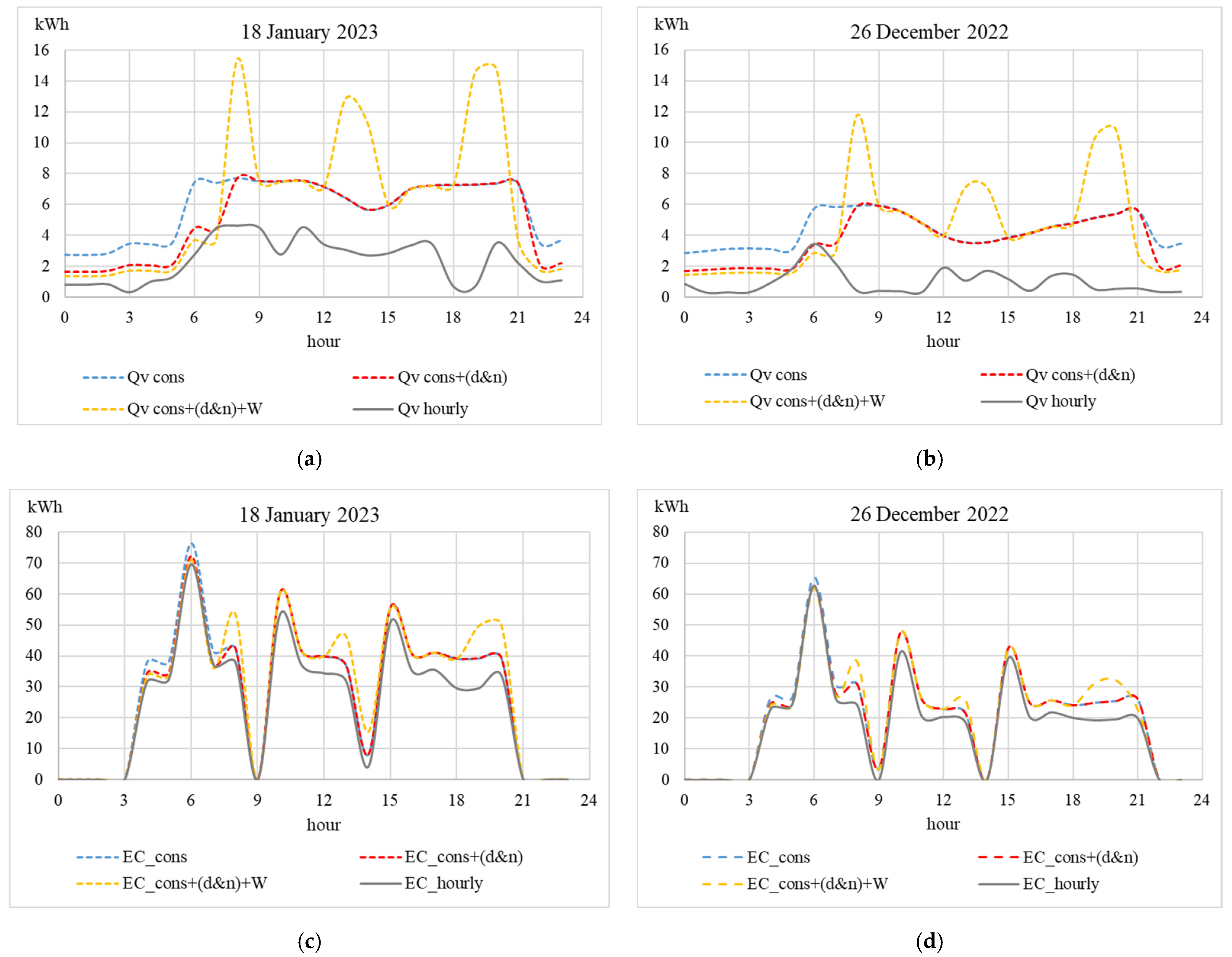
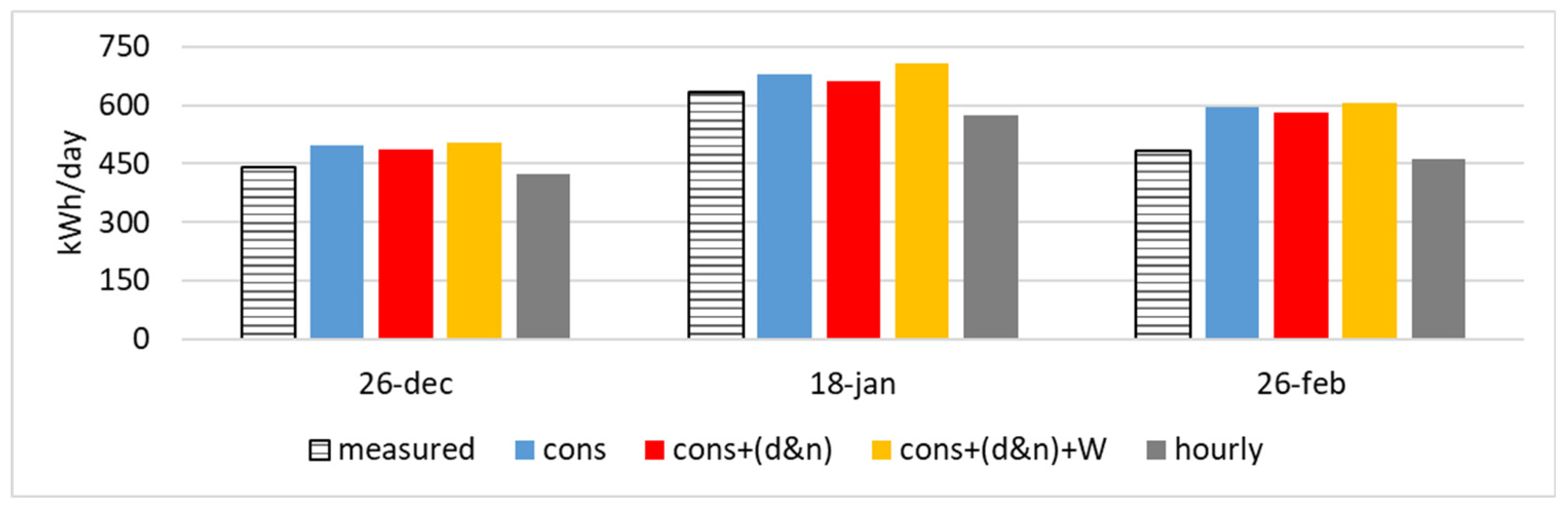
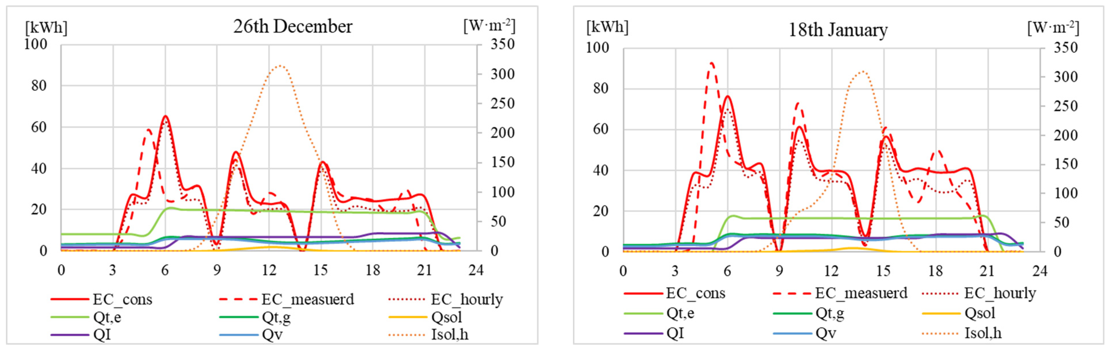
4.4.2. Application Results
5. Conclusions
Author Contributions
Funding
Data Availability Statement
Conflicts of Interest
References
- IEA. Buildings—Energy System. Available online: https://www.iea.org/energy-system/buildings (accessed on 28 January 2025).
- NREL Researchers Reveal How Buildings Across United States Do—and Could—Use Energy. Available online: https://www.nrel.gov/news/features/2023/nrel-researchers-reveal-how-buildings-across-the-united-states-do-and-could-use-energy.html (accessed on 28 January 2025).
- U.S Department of Energy. Building Energy Modeling. Available online: https://www.energy.gov/eere/buildings/building-energy-modeling (accessed on 28 January 2025).
- Ali, U.; Shamsi, M.H.; Hoare, C.; Mangina, E.; O’Donnell, J. Review of urban building energy modeling (UBEM) approaches, methods and tools using qualitative and quantitative analysis. Energy Build. 2021, 246, 111073. [Google Scholar] [CrossRef]
- Kamel, E. A Systematic Literature Review of Physics-Based Urban Building Energy Modeling (UBEM) Tools, Data Sources, and Challenges for Energy Conservation. Energies 2022, 15, 8649. [Google Scholar] [CrossRef]
- Mutani, G.; Todeschi, V.; Beltramino, S. Energy Consumption Models at Urban Scale to Measure Energy Resilience. Sustainability 2020, 12, 5678. [Google Scholar] [CrossRef]
- Javanroodi, K.; Mahdavinejad, M.; Nik, V.M. Impacts of urban morphology on reducing cooling load and increasing ventilation potential in hot-arid climate. Appl. Energy 2018, 231, 714–746. [Google Scholar] [CrossRef]
- Santantonio, S.; Mutani, G. QGIS-Based Tools to Evaluate Air Flow Rate by Natural Ventilation in Buildings at Urban Scale. In Proceedings of the BSA Conference 2022 IBPSA-Italy, Bozen-Bolzano, Italy, 29 June–1 July 2022; Volume 5, pp. 331–339. Available online: https://publications.ibpsa.org/conference/paper/?id=bsa2022_9788860461919_42 (accessed on 6 January 2025).
- Todeschi, V.; Boghetti, R.; Kämpf, J.H.; Mutani, G. Evaluation of Urban-Scale Building Energy-Use Models and Tools—Application for the City of Fribourg, Switzerland. Sustainability 2021, 13, 1595. [Google Scholar] [CrossRef]
- Dabirian, S.; Panchabikesan, K.; Eicker, U. Occupant-centric urban building energy modeling: Approaches, inputs, and data sources—A review. Energy Build. 2022, 257, 111809. [Google Scholar] [CrossRef]
- Taddeo, P.; Ortiz, J.; Salom, J.; Segarra, E.L.; González, G.V.; Ruiz, G.R.; Bandera, C.F. Comparison of Experimental Methodologies to Estimate the Air Infiltration Rate in a Residential Case Study for Calibration Purposes, 2018. Available online: https://www.semanticscholar.org/paper/Comparison-of-experimental-methodologies-to-the-air-Taddeo-Ortiz/437eab49b3304179d102167876f74733caff6be4 (accessed on 28 January 2025).
- Santantonio, S.; Dell’Edera, O.; Moscoloni, C.; Bertani, C.; Bracco, G.; Mutani, G. Wind-driven and buoyancy effects for modeling natural ventilation in buildings at urban scale. Energy Effic. 2024, 17, 95. [Google Scholar] [CrossRef]
- National Institute of Standards and Technology. CONTAM Introduction. Available online: https://www.nist.gov/el/energy-and-environment-division-73200/nist-multizone-modeling/software/contam (accessed on 15 December 2024).
- Ng, L.C.; Musser, A.; Persily, A.K.; Emmerich, S.J. Airflow and Indoor Air Quality Models of DOE Prototype Commercial Buildings; National Institute of Standards and Technology: Gaithersburg, MD, USA, 2019. [Google Scholar] [CrossRef]
- Dols, W.S.; Polidoro, B. CONTAM User Guide and Program Documentation Version 3.4; National Institute of Standards and Technology: Gaithersburg, MD, USA. Available online: https://www.nist.gov/publications/contam-user-guide-and-program-documentation-version-34 (accessed on 18 December 2024).
- Haghighat, F.; Megri, A.C. A Comprehensive Validation of Two Airflow Models—COMIS and CONTAM. Indoor Air 1996, 6, 278–288. [Google Scholar] [CrossRef]
- Chung, K.-C. Development and Validation of a Multizone Model for Overall Indoor Air Environment Prediction. HVAC&R Res. 1996, 2, 376–385. [Google Scholar] [CrossRef]
- Emmerich, S.J.; Howard-Reed, C.; Nabinger, S. Validation of multizone IAQ model predictions for tracer gas in a townhouse. Build. Serv. Eng. Res. Technol. 2004, 25, 305–316. [Google Scholar] [CrossRef]
- Emmerich, S.J. Validation of Multizone IAQ Modeling of Residential-Scale Buildings: A Review; No. Pt.2; National Institute of Standards and Technology: Gaithersburg, MD, USA, 2001; Volume 107. Available online: https://www.nist.gov/publications/validation-multizone-iaq-modeling-residential-scale-buildings-review (accessed on 18 December 2024).
- Ng, L.C.; Zimmerman, S.M.; Good, J.; Tool, B.; Emmerich, S.; Persily, A. Estimating Real-Time Infiltration for Use in Residential Ventilation Control; National Institute of Standards and Technology: Gaithersburg, MD, USA, 2019. Available online: https://www.nist.gov/publications/estimating-real-time-infiltration-use-residential-ventilation-control (accessed on 18 December 2024).
- IEA. Annex 23—An International Effort in Multizone Air Flow Modeling | Smarter Small Buildings. Available online: https://smartersmallbuildings.lbl.gov/publications/annex-23-international-effort (accessed on 18 March 2025).
- RDH Building Science, Study of Part 3 Building Airtightness. Available online: https://www.rdh.com/resource/study-of-part-3-building-airtightness/ (accessed on 9 December 2024).
- UNI EN 12207:2017—UNI Ente Italiano di Normazione. Available online: https://store.uni.com/uni-en-12207-2017 (accessed on 17 November 2024).
- Mckeen, P.; Liao, Z. The Influence of Building Airtightness on Airflow in Stairwells. Buildings 2019, 9, 208. [Google Scholar] [CrossRef]
- UNI/TS 11300-1:2014 —Determinazione del Fabbisogno di Energia Termica Dell’edificio per la Climatizzazione Estiva ed Invernale. Available online: https://store.uni.com/uni-ts-11300-1-2014 (accessed on 15 November 2024). (In Italian).
- EnergyPlus. Available online: https://energyplus.net/weather-location/north_and_central_america_wmo_region_4/USA/FL/USA_FL_Southwest.Florida.Intl.AP.722108_TMY3 (accessed on 16 December 2024).
- National Institute of Standards and Technology. CONTAM Weather File Creator 2.0. 2018. Available online: https://www.nist.gov/el/energy-and-environment-division-73200/nist-multizone-modeling/software/contam-weather-file (accessed on 24 January 2025).
- Florida Solar Energy Center; Chandra, S. Procedures for Calculating Natural Ventilation Airflow Rates in Buildings. 03-87. FSEC Energy Research Center®, 1987. Available online: https://stars.library.ucf.edu/fsec/988 (accessed on 16 December 2024).
- Kent, C.W.; Lindberg, F.; Offerle, B.; Grimmond, S.; Krave, N. Urban Morphology and Morphometric Calculator (Grid), UMEP Documentation, 2023. Available online: https://umep-docs.readthedocs.io/en/latest/pre-processor/Urban%20Morphology%20Morphometric%20Calculator%20%28Grid%29.html (accessed on 17 February 2025).
- Kent, C.W.; Grimmond, S.; Barlow, J.; Gatey, D.; Kotthaus, S.; Lindberg, F.; Halios, C.H. Evaluation of Urban Local-Scale Aerodynamic Parameters: Implications for the Vertical Profile of Wind Speed and for Source Areas. Bound.-Layer Meteorol. 2017, 164, 183–213. [Google Scholar] [CrossRef] [PubMed]
- Kanda, M.; Inagaki, A.; Miyamoto, T.; Gryschka, M.; Raasch, S. A New Aerodynamic Parametrization for Real Urban Surfaces. Bound.-Layer Meteorol. 2013, 148, 357–377. [Google Scholar] [CrossRef]
- Javanroodi, K.; Nik, V.M. Interactions between extreme climate and urban morphology: Investigating the evolution of extreme wind speeds from mesoscale to microscale. Urban Clim. 2020, 31, 100544. [Google Scholar] [CrossRef]
- Feustel, H.E. COMIS—An international multizone air-flow and contaminant transport model. Energy Build. 1999, 30, 3–18. [Google Scholar] [CrossRef]
- Fsolve. Available online: https://it.mathworks.com/help/optim/ug/fsolve.html (accessed on 10 January 2025).
- Emmerich, S.J.; Persily, A.; Mcdowell, T. Impact of Infiltration on Heating and Cooling Loads in U.S. Office Buildings, Building and Fire Research Laboratory, National Institute of Standards and Technology. Available online: https://www.researchgate.net/publication/265919110_Impact_of_Infiltration_on_Heating_and_Cooling_Loads_in_US_Office_Buildings (accessed on 10 January 2025).
- Emmerich, S.J.; Persily, A.K. U.S commercial building airtightness requirements and measurements. In Proceedings of the AIVC Conference 2011, Brussels, Belgium, 12–13 October 2011; Available online: https://www.aivc.org/resource/us-commercial-building-airtightness-requirements-and-measurements (accessed on 30 January 2025).
- Herring, S.J.; Batchelor, S.; Bieringer, P.E.; Lingard, B.; Lorenzetti, D.M.; Parker, S.T.; Rodriguez, L.; Sohn, M.D.; Steinhoff, D.; Wolski, M. Providing pressure inputs to multizone building models. Build. Environ. 2016, 101, 32–44. [Google Scholar] [CrossRef]
- LivingLAB@polito.it—Ambiente Esterno. Available online: https://smartgreenbuilding.polito.it/monitoraggio/esterno.asp (accessed on 16 December 2024).


| Envelope (walls, floors, roof): Powerlaw Model: Leakage area | |||
| Prototype | Turin | ||
| Leakage per unit area [cm2/m2] | 2.208 | 1.783 | |
| Discharge coefficient [-] | 1 | 1 | |
| Flow exponent [-] | 0.65 | 0.65 | |
| Pressure difference [Pa] | 4 | 4 | |
| Internal doors | |||
| Prototype | Turin | ||
| Apartment/shaft doors: Powerlaw Model: Orifice | Internal doors (within apartments): Two-way Model: Single-opening | ||
| Cross-sectional area [m2] | 0.023 | Height [m] | 2.2 |
| Flow exponent [-] | 0.5 | Width [m] | 0.9 |
| Discharge coefficient [-] | 0.6 | Discharge coefficient [-] | 0.78 |
| Hydraulic diameter [m] | 0.172 | Apartment/shaft doors: Powerlaw Model: F = C(ΔP)n | |
| Reynold number [-] | 30 | Flow coefficient (C) [-] | Equation (2) |
| Flow exponent (n) [-] | 0.65 | ||
| Season | Temperature [°C] | |
|---|---|---|
| Heated Zones (a&b) | Shaft (Zone c) | |
| Winter | 20 | |
| Summer | 26 | |
| Winter | Summer | |||||||||
|---|---|---|---|---|---|---|---|---|---|---|
| Tout [°C] | −10 | −5 | 0 | 3 | 7 | 12 | 24 | 28 | 30 | 34 |
| Ws [m/s] | 0.1, 0.5, 1 → 10 (with an increment of 1 for each simulation) | |||||||||
| [°C] | Tout | −10 | −5 | 0 | 3 | 7 | 12 | 24 | 28 | 30 | 34 |
| Tin | 20 | 26 | |||||||||
| Tshaft | 2 | 5 | 8 | 9.8 | 12.2 | 15.2 | 24.8 | 27.2 | 28.4 | 30.8 | |
| ΔT |Tout − Tin| | 30 | 25 | 20 | 17 | 13 | 8 | 2 | 2 | 4 | 8 | |
| Wind speed [m/s] | 0.1 | 0.0005 | 0.0004 | 0.0016 | 0.0026 | 0.0044 | 0.0071 | 0.0128 | 0.0159 | 0.0154 | 0.0151 |
| 0.5 | 0.0005 | 0.0004 | 0.0016 | 0.0017 | 0.0005 | 0.0007 | 0.0063 | 0.0095 | 0.0106 | 0.0132 | |
| 1 | 0.0036 | 0.0023 | 0.0008 | 0.0002 | 0.0019 | 0.0023 | 0.0053 | 0.0066 | 0.0103 | 0.0067 | |
| 2 | 0.0132 | 0.0108 | 0.0049 | 0.0066 | 0.0047 | 0.0030 | 0.0036 | 0.0042 | 0.0049 | 0.0066 | |
| 3 | 0.0309 | 0.0107 | 0.0056 | 0.0092 | 0.0081 | 0.0075 | 0.0006 | 0.0013 | 0.0021 | 0.0037 | |
| 4 | 0.0099 | 0.0156 | 0.0120 | 0.0128 | 0.0120 | 0.0111 | 0.0053 | 0.0027 | 0.0016 | 0.0004 | |
| 5 | 0.0408 | 0.0168 | 0.0179 | 0.0171 | 0.0160 | 0.0149 | 0.0081 | 0.0079 | 0.0066 | 0.0039 | |
| 6 | 0.0457 | 0.0243 | 0.0225 | 0.0216 | 0.0203 | 0.0189 | 0.0101 | 0.0093 | 0.0090 | 0.0085 | |
| 7 | 0.0448 | 0.0294 | 0.0274 | 0.0263 | 0.0248 | 0.0231 | 0.0122 | 0.0112 | 0.0107 | 0.0098 | |
| 8 | 0.0373 | 0.0349 | 0.0326 | 0.0313 | 0.0296 | 0.0275 | 0.0145 | 0.0132 | 0.0126 | 0.0114 | |
| 9 | 0.0434 | 0.0406 | 0.0379 | 0.0364 | 0.0344 | 0.0321 | 0.0168 | 0.0153 | 0.0146 | 0.0132 | |
| 10 | 0.0496 | 0.0465 | 0.0435 | 0.0417 | 0.0395 | 0.0368 | 0.0193 | 0.0176 | 0.0167 | 0.0151 | |
| WALL | ROOF | GROUND | GLAZING | ACR | η | ||||
|---|---|---|---|---|---|---|---|---|---|
| Period | Cenvelope | Uwall | Uroof | Ufloor | Ug | WWR | g-Value | h−1 | |
| kJ·m−2·K−1 | W·m−2·K−1 | W·m−2·K−1 | W·m−2·K−1 | W·m−2·K−1 | - | - | - | - | |
| <1918 | 504 | 1.45 | 1.80 | 1.75 | 4.85 | 0.13 | 0.85 | 0.5 | 0.78 |
| 1919–45 | 504 | 1.35 | 1.80 | 1.58 | 4.75 | 0.13 | 0.85 | 0.5 | 0.78 |
| 1946–60 | 283 | 1.18 | 1.80 | 1.23 | 4.40 | 0.20 | 0.85 | 0.5 | 0.78 |
| 1961–70 | 283 | 1.13 | 2.20 | 1.30 | 4.90 | 0.20 | 0.85 | 0.5 | 0.79 |
| 1971–80 | 257 | 1.04 | 2.20 | 1.00 | 3.80 | 0.25 | 0.75 | 0.5 | 0.80 |
| 1981–90 | 264 | 0.78 | 1.18 | 0.95 | 3.80 | 0.20 | 0.75 | 0.5 | 0.82 |
| 1991–00 | 274 | 0.7 | 0.68 | 0.80 | 2.15 | 0.20 | 0.67 | 0.5 | 0.84 |
| 2001–05 | 274 | 0.7 | 0.68 | 0.80 | 2.15 | 0.20 | 0.67 | 0.3 | 0.84 |
| 2006–12 | 267 | 0.42 | 0.38 | 0.41 | 2.60 | 0.20 | 0.50 | 0.3 | 0.92 |
| 2013–15 | 267 | 0.34 | 0.30 | 0.33 | 2.20 | 0.20 | 0.50 | 0.3 | 0.92 |
| 2016–19 | 267 | 0.30 | 0.25 | 0.30 | 1.80 | 0.20 | 0.35 | 0.3 | 0.92 |
| Scenario | Building Permeability | ACR | |
|---|---|---|---|
| 1 | cons | Based on construction period | 0.5 constant during the day |
| 2 | cons+(d&n) | Same as 1, with less permeability during the night for window shutters | 0.5 during the day and 0.3 during the nigh |
| 3 | cons+(d&n)+W | Same as 2, with additional window opening for three times of the day | For 3 h, with windows opening, ACR was calculated by a correlation [6] considering 15 min of windows opening |
| 4 | hourly | Air infiltration depends on the weather conditions. It was considered an average airtightness of masonry buildings, i.e., 4.58 L/s/m2 @75 | ACR was calculated from the three-zone lumped-parameter model in each hour of the year |
| Scenario | 26-Dec | 18-Jan | 26-Feb |
|---|---|---|---|
| cons | 12.6% | 7.2% | 22.9% |
| cons+(d&n) | 10.3% | 4.7% | 19.6% |
| cons+(d&n)+W | 14.5% | 11.9% | 25.4% |
| hourly | 4.3% | 7.6% | 4.7% |
| Tout [°C] | 6.83 | 5.44 | 5.96 |
| Ws [m/s] | 1.88 | 0.97 | 1.93 |
Disclaimer/Publisher’s Note: The statements, opinions and data contained in all publications are solely those of the individual author(s) and contributor(s) and not of MDPI and/or the editor(s). MDPI and/or the editor(s) disclaim responsibility for any injury to people or property resulting from any ideas, methods, instructions or products referred to in the content. |
© 2025 by the authors. Licensee MDPI, Basel, Switzerland. This article is an open access article distributed under the terms and conditions of the Creative Commons Attribution (CC BY) license (https://creativecommons.org/licenses/by/4.0/).
Share and Cite
Usta, Y.; Ng, L.; Santantonio, S.; Mutani, G. Lumped-Parameter Models Comparison for Natural Ventilation Analyses in Buildings at Urban Scale. Energies 2025, 18, 2352. https://doi.org/10.3390/en18092352
Usta Y, Ng L, Santantonio S, Mutani G. Lumped-Parameter Models Comparison for Natural Ventilation Analyses in Buildings at Urban Scale. Energies. 2025; 18(9):2352. https://doi.org/10.3390/en18092352
Chicago/Turabian StyleUsta, Yasemin, Lisa Ng, Silvia Santantonio, and Guglielmina Mutani. 2025. "Lumped-Parameter Models Comparison for Natural Ventilation Analyses in Buildings at Urban Scale" Energies 18, no. 9: 2352. https://doi.org/10.3390/en18092352
APA StyleUsta, Y., Ng, L., Santantonio, S., & Mutani, G. (2025). Lumped-Parameter Models Comparison for Natural Ventilation Analyses in Buildings at Urban Scale. Energies, 18(9), 2352. https://doi.org/10.3390/en18092352