Modeling the Electricity Generation Processes of a Combined Solar and Small Hydropower Plant

Abstract

This article proposes the concept of an integrated system consisting of two components: a small hydropower plant (SHPP) and a solar power plant (SPP), where the SHPP operates as a pumped-storage hydropower plant, and the SPP supplies energy for lifting water to the upper reservoir. A methodology is proposed for evaluating the joint operation of a solar power plant and a small hydropower plant. The methodology is based on modeling the electricity generation processes of combined solar and small hydropower plants. Additionally, a novel hybrid method is proposed for identifying interval models of small hydropower plants (SHPPs) and solar power plants (SPPs). This method integrates a metaheuristic algorithm for model structure synthesis, inspired by the behavioral model of a bee colony, with gradient-based methods for parameter identification. Using the proposed method, interval models have been developed for both small hydropower plants and the electricity generation of solar power plants. This study confirms the feasibility of using interval models to describe the relationship between electricity generation in a small hydropower plant and factors such as head difference, reactive power, and water level in the reservoir (i.e., available water resources). Furthermore, a mathematical model in the form of a difference equation is used to describe the daily electricity generation of a solar power plant. This model accounts for the characteristics of compressors that pump water from the lower to the upper reservoir. Based on the developed models, an assessment is conducted on the efficiency of the pumped-storage SHPP in ensuring operational stability during peak loads in the power grid and addressing seasonal variations.

1. Introduction

The problem of providing electricity in Ukraine is becoming increasingly urgent. First of all, this is due to the full-scale invasion of the Russian Federation in Ukraine. The destruction of energy infrastructure and the loss of control over the occupied territories has led to obstacles to ensuring the uninterrupted supply of electricity to the population. Moreover, the problem has global trends. Many countries are intensively looking for alternative energy sources. Taking into account the negative consequences for the environment from the use of traditional energy in order to ensure sustainable development [1,2,3].

The tendency to reduce dependence on fossil fuels is growing due to the use of alternative energy, namely, solar energy, hydropower, and bioenergy [4,5,6]. The potential of solar energy primarily lies in the ability to meet the global energy needs of mankind through an environmentally friendly, renewable energy source. In particular, the advantages of introducing solar energy include the economic efficiency of electricity generated, reduction of greenhouse gas emissions into the environment, energy security and independence from fossil fuel imports, absence of noise pollution, and accessibility [7,8,9]. However, in addition to the advantages, there are also disadvantages of using solar energy. The following disadvantages of solar energy should be noted: dependence on weather conditions, high initial costs, the need for large areas of land, the problem of the utilization of used panels, and, the main problem, the accumulation of generated electricity to balance the operating modes of the power system [8,9,10].

Recently, scientists in the field of alternative energy have solved these problems by using various sources of accumulation and generation [11,12,13,14,15]. In particular, many systems have been developed that combine the generation of solar, wind, and hydropower plants [16,17,18]. The main objectives of such integration are to ensure the stability of the power system and to focus on compensating for peak loads.

2. A Review of Tasks and Methods for Modeling the Joint Operation of an SHPP and an SPP

Taking into account the growing share of renewable energy sources in the structure of modern energy systems, combined-cycle power plants are increasingly becoming an object of research [19,20,21,22,23].

Modeling is a critically important tool for analyzing, designing, and optimizing hybrid electricity generation systems. Modern research employs a wide range of methods that account for the following factors:

• the dynamic behavior of systems;
• the integration of various energy sources;
• thermodynamic processes;
• electromechanical phenomena.

Dynamic modeling enables the analysis of system performance over time, accounting for external conditions and operational parameters [24,25]. This method provides accurate predictions of hybrid system behavior under varying load conditions and deviations from design specifications.

In paper [26], a dynamic mathematical model for an integrated solar combined-cycle power plant operating under off-design conditions is developed. Implemented in MATLAB, the model incorporates real meteorological data and operational parameters to simulate the influence of solar irradiance and wind speed on system performance. The results demonstrate high predictive accuracy, with root mean square errors below 5%, providing valuable insights for operational control strategies.

In paper [27], a sophisticated dynamic simulation model for an integrated solar combined-cycle power plant using APROS 6.09 software is validated. The model accurately predicts operational performance under varying conditions, highlighting its utility for grid-stability planning and operational decision-making. These studies underscore the importance of dynamic modeling for enhancing the adaptability and resilience of hybrid energy systems.

The integration of multiple energy sources in a single system requires modeling their interaction to optimize overall performance. These models take into account the production characteristics of each energy source (solar, wind, small hydropower).

The integration of SHPP and SPP can be implemented in various ways, depending on technical, economic, and climatic conditions. In particular, in [28], photovoltaic panels are installed on floating structures. Such a system is located on the Indus River (Pakistan) at the Ghazi Barotha hydroelectric power station. The existing hydroelectric power station generates 1450 MW, and photovoltaic installations generate 200 MW. The proposed system generates an additional 3.5% of electricity. The integrated operation of the hydroelectric power station and photovoltaic panels helps to reduce the electricity deficit in the network.

In works [29,30,31], scientists described the principles of the optimal use of interlocked systems to reduce electricity shortages and analyzed the principles of complementarity between SHPP and SPP.

The authors of paper [32] studied the interlocked operation of hybrid pumped storage hydropower plants with wind and photovoltaic installations in the Wujiang River basin, China. A model for integrating these energy sources is proposed to increase the efficiency of renewable resources, ensure the stability of the power system, and reduce the impact of fluctuations in generation from renewable energy sources. Different strategies for the proposed interlocked system are studied. It was found that this hybrid system in the Wujiang River basin can increase the profit from electricity production and reduce electricity shortages. It should be noted that, in paper [32], a pumping station is used, which increases the amount of available water during the dry season.

In papers [33,34,35,36,37,38], a detailed Matlab-based model for a distributed hybrid system integrating solar, wind, and small hydro sources is presented. By combining 3 MW of hydropower with 1 MW each of solar and wind power, the study demonstrated improved energy reliability and cost-effectiveness, with electricity generation costs significantly lower than conventional.

Many studies by scientists on the joint operation of hydropower plants and solar power plants are aimed at optimizing the operation of these systems, compensating for seasonal fluctuations, conducting an analysis of the economic feasibility of creating hybrid plants, and assessing the state of the environment. Among such works, one should consider [34], which was considered in Taiwan. For the optimization of electricity, the authors of [34] proposed a multi-objective optimization model based on the Grasshopper optimization algorithm. The Grasshopper model is aimed at the optimal construction of the design of a blocked system, and not at studying the processes of forming potential energy by using the gravitational force of spent hydro resources.

Yusheng Zhang et al. [35] investigated an innovative method for the optimal sizing of interlocked hydropower and solar power systems considering the dynamics of electricity demand and reservoir parameters. The simulation results were applied to an interlocked system in Qinghai province, China, using GA and MATLAB R2023b software.

The authors of works [38,39,40,41] investigate the state of the modeling of hybrid renewable energy systems. In particular, they analyze methods for modeling the efficiency of hybrid plants and predicting their reliable integration.

In [42], a hybrid pumped and battery storage (HPBS) system is proposed to enhance the reliability of off-grid renewable energy systems by optimizing storage utilization. The model prioritizes pumped hydro storage for high energy demands while using batteries only for minor shortfalls. A control strategy based on the operating range of a reversible pump-turbine maximizes efficiency, as validated through simulations. Key performance metrics show a system-wide energy utilization ratio of 16.5%, with high efficiency in both storage types. The study highlights HPBS as a sustainable solution for balancing renewable energy supply and demand.

Thermodynamic models provide critical insights into the energy conversion processes and efficiency of hybrid power systems. In paper [43], a detailed analysis of the thermodynamic characteristics and economic aspects of a combined solar system incorporating parabolic trough collectors is conducted. Their simulations revealed that increasing solar field aperture significantly enhances system efficiency, albeit with diminishing economic returns at larger scales. These models aid in the design of more efficient and economically viable renewable energy systems.

SHPPs play a vital role in decentralized energy generation, requiring sophisticated modeling to address electromagnetic phenomena and prognose their dynamics. In paper [44], a simulation model is developed to analyze the electro-mechanical behavior of SHPs during start-up and grid connection. The study identified critical factors influencing peak currents and proposed solutions to minimize these effects, ensuring system stability and reliability. This work highlights the importance of precise modeling in optimizing the performance of SHPP and reducing operational risks.

Recent advancements in modeling hybrid energy systems emphasize the importance of dynamic, thermodynamic, and hybrid integration approaches for optimizing renewable energy generation. From predictive simulations of solar–hydro systems to electro-mechanical analyses of SHPs, these studies contribute to the ongoing transition toward more sustainable and efficient energy solutions.

Based on the research conducted, the following conclusions can be drawn. The functioning of interlocked systems makes it possible to solve many problems, including the following:

• increasing the efficiency of the operation of interlocked SHPP and SPP systems (by using SPP energy to replenish additional hydro resources for SHPP electricity production);
• large-scale electricity accumulation due to potential energy generated by the gravitational force of water.

The novelty of this study lies in the development of: a concept for the integrated operation of SHPPs and SPPs, where the generated power from SPPs is used for hydro accumulation in SHPPs by pumping water resources into the upper reservoir; mathematical models for evaluating the efficiency of the integrated operation of SHPPs and SPPs based on the existing hydrotechnical characteristics of SHPPs and the capacity of SPPs at the design stage; and the advancement of methods for identifying nonlinear static and dynamic models based on interval data.

3. Materials and Methods

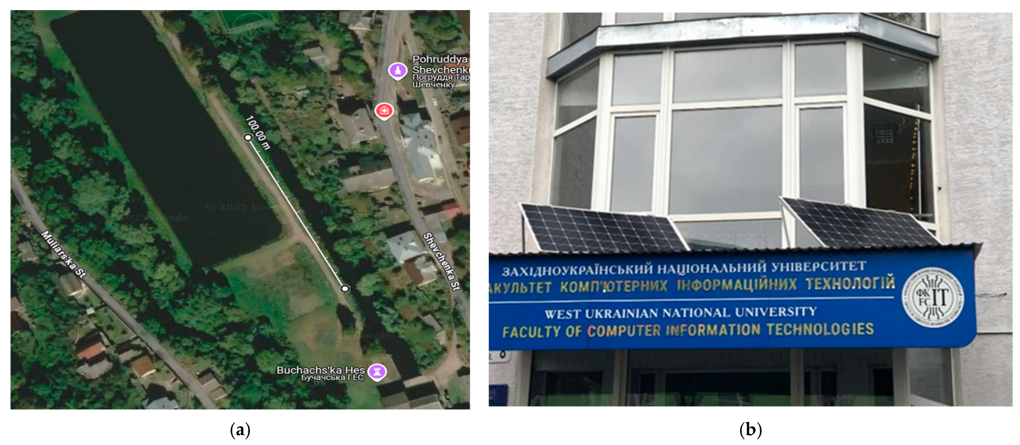
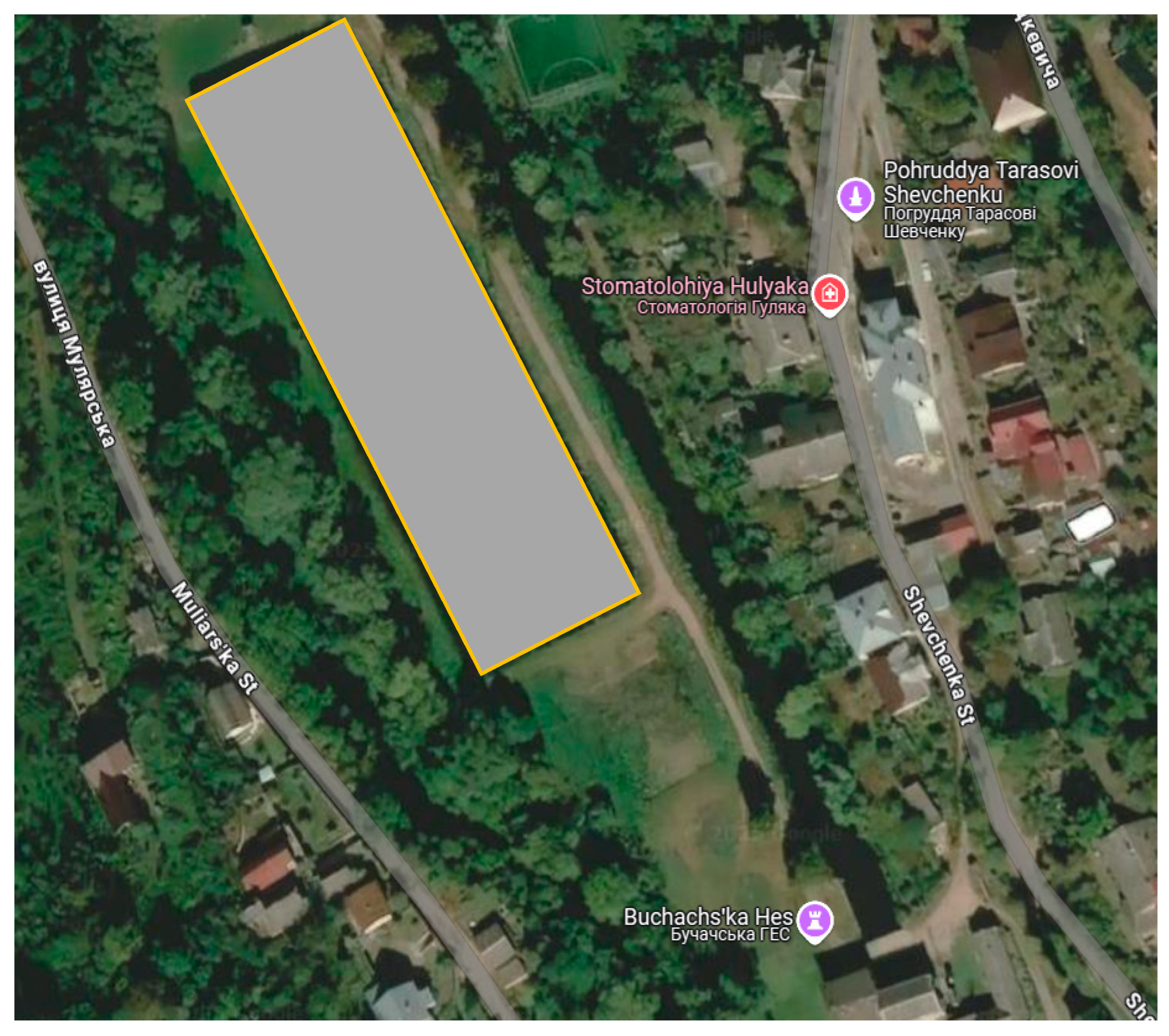
3.1. Concept of Joint Operation of a Solar Power Plant and a Small Hydropower Plant

Now, consider the case where the electricity generation of a small hydropower plant (SHPP) is enhanced by supplementing hydro resources through the operation of a solar power plant (SPP). The schematic representation of the combined operation of both plants is shown in Figure 1.

As seen in Figure 1, the SHPP generates electricity by utilizing the gravitational force of water accumulated in the upper bier. The electricity generation process depends on the input factor vector ${\overrightarrow{X}}_i$, particularly, the head difference and the water flow rate through the hydro turbine. These factors, in turn, are determined by the volume of water in the upper bier.

There are two ways to increase the generated power: increasing the water flow rate through the turbine and raising the water level in the upper bier. In this system, the electricity generated by the SPP is directly used to replenish the water volume available for the SHPP. This is achieved by supplying the electricity produced by the SPP to power electric pumps that transfer water from the lower bier to the upper one. Therefore, to model and optimize the joint operation of an SHPP and an SPP, it is necessary to develop and integrate three mathematical models, as depicted in Figure 1: model of the small hydropower plant, model of the solar power plant, and model of the additional hydro resources obtained. All three models are constructed based on experimental data derived from interval data analysis. This approach offers two key benefits: it enhances electricity generation in the SHPP, particularly during peak load periods in the power grid, and it enables the accumulation of electricity generated by the SPP.

3.2. The Task Statement

The main factors at a small hydro power plant (SHPP) that affect the amount of generated electricity are head difference, reactive power, and the water level in the reservoir, that is, the available hydraulic resources. It is on this basis that the mathematical model of the SHPP will be built. Such a model is interval since, when preparing data for its identification, the generated electricity is measured with errors according to a given accuracy. Further, using a mathematical model that describes the amount of electricity generated by a solar power plant during the day, taking into account the characteristics of compressors pumping water from the lower reservoir to the upper reservoir, the possible value of the upper reservoir installation is estimated. Substituting this value into the model of the volume of generated electricity using the SHPP, we obtain the value of the generated electricity of the system.

Consider the formulation of the problem of constructing a mathematical model to reflect the relationship between the daily amount of generated electricity and a vector $\overrightarrow{X}$ of factors that determines the characteristics of hydraulic equipment and available hydraulic resources. Denote by $y(\overrightarrow{\beta },\overrightarrow{X})$ the daily amount of generated electricity depending on the vector $\overrightarrow{X}$.

In this case, we consider the static characteristic, and the above dependence is described by the following algebraic equation:

$$y\left(\overrightarrow{\beta },\overrightarrow{X}\right)=f_1\left(\overrightarrow{\beta },\overrightarrow{X}\right)+...+f_m\left(\overrightarrow{\beta },\overrightarrow{X}\right),$$

(1)

where $y(\overrightarrow{\beta },\overrightarrow{X})$ means the daily amount of generated electricity; $\overrightarrow{\beta }$ is a vector of unknown model parameters; and $f_1(\overrightarrow{\beta },\overrightarrow{X}),...,f_m(\overrightarrow{\beta },\overrightarrow{X})$ denotes a set of nonlinear basis functions, which, as we see, depend on the vector of input variables $\overrightarrow{X}$ and on the vector of parameters $\overrightarrow{\beta }$ of the model.

The results of the experiment, which are necessary to identify the parameters of the nonlinear model, are presented in this form [45]:

$${\overrightarrow{X}}_i\to \left[y_i^{-};y_i^{+}\right],\hspace{0.33em}i=\overline{1,N},$$

(2)

where $[y_i^{-};y_i^{+}]$ are lower and upper limits of experimentally obtained values of the daily generated electric power of the i-th conditions of measurement, which are determined by vector ${\overrightarrow{X}}_i$, for each $i=\overline{1,N}$ measurements.

In this case, the problem of the parametric identification of the model in the form of Expression (2) is to estimate the values of the $\overrightarrow{\stackrel{̑}{\beta }}$ parameter vector. The presence of these estimates makes it possible to obtain a mathematical model with a reflection of the relationship between the daily amount of electricity generated and the vector $\overrightarrow{X}$ of factors that determine the characteristics of hydraulic equipment and available hydraulic resources:

$${\stackrel{̑}{y}}_i\left(\overrightarrow{\stackrel{̑}{\beta }},{\overrightarrow{X}}_i\right)=f_1\left(\overrightarrow{\stackrel{̑}{\beta }},{\overrightarrow{X}}_i\right),...,+f_m\left(\overrightarrow{\stackrel{̑}{\beta }},{\overrightarrow{X}}_i\right),i=\overline{1,N}.$$

(3)

For the above problem, $\stackrel{̑}{y}(\overrightarrow{\stackrel{̑}{\beta }},\overrightarrow{X})$ refers to the computed daily amount of electricity generated. Based on the requirements for ensuring a given accuracy of the model, which are used in the analysis of interval data, we can state that the simulated values describe the daily generated volume of SHPP electricity, which must belong to numerical intervals that are obtained experimentally. That is, when determining parameter estimates, the following conditions must be met for the resulting model:

$${\stackrel{̑}{y}}_i\left(\overrightarrow{\stackrel{̑}{\beta }},{\overrightarrow{X}}_i\right)\in \left[y_i^{-};y_i^{+}\right], i=\overline{1,N}.$$

(4)

From here, substituting in Conditions (4) instead of $\stackrel{̑}{y}\left(\overrightarrow{\stackrel{̑}{\beta }},{\overrightarrow{X}}_i\right)$ in Expression (3), we obtain the conditions for evaluating the parameters of the model $\overrightarrow{\stackrel{̑}{\beta }}$:

$$y_i^{-}\le f_1\left(\overrightarrow{\stackrel{̑}{\beta }},{\overrightarrow{X}}_i\right)+\dots +f_m\left(\overrightarrow{\stackrel{̑}{\beta }},{\overrightarrow{X}}_i\right)\le y_i^{+}, i=\overline{1,N}.$$

(5)

The obtained System (5) is an interval system of nonlinear algebraic equations (ISNAE) for unknown estimates of the parameter vector [20,45,46,47]. A set of ISNAE solutions defines a set of vectors of estimates of model parameters.

Due to the high (combinatorial) computational complexity of solving this ISNAE, only point estimates of the parameters are calculated in practice. In this case, the optimization problem is solved to estimate the parameters as follows [45,46,47]:

$$\delta \left(\overrightarrow{\stackrel{̑}{\beta }}\right)\stackrel{\hspace{1em}\overrightarrow{\stackrel{̑}{\beta }},{\alpha }_i\hspace{1em}}{\to }min, \overrightarrow{\stackrel{̑}{\beta }}\in \left[{\overrightarrow{\stackrel{̑}{\beta }}}^{low};{\overrightarrow{\stackrel{̑}{\beta }}}^{up}\right], {\alpha }_i\in [\mathrm{0,1}], i=\overline{1,N}.$$

(6)

where ${\alpha }_i$ is the linear combination coefficients for determining a point within the experimental data $[y_i^{-};y_i^{+}]$, which are added to ensure the smoothness of the objective function.

The objective function in this case is as follows [19,47,48]:

$$\begin{gathered} \delta \left(\overrightarrow{\stackrel{̑}{\beta }}\right)=\sum _{i=1}^N{\left({\widehat{y}}_i\left(\overrightarrow{\stackrel{̑}{\beta }},{\overrightarrow{X}}_i\right)-P\left(\left[y_i^{-};y_i^{+}\right], {\alpha }_i\right) \right)}^2 \\ =\sum _{i=1}^N{\left(f_1\left(\overrightarrow{\stackrel{̑}{\beta }},{\overrightarrow{X}}_i\right)+\dots +f_m\left(\overrightarrow{\stackrel{̑}{\beta }},{\overrightarrow{X}}_i\right)-\left({\alpha }_i\cdot y_i^{-}+\left(1-{\alpha }_i\right)\cdot y_i^{+}\right)\right)}^2. \end{gathered}$$

(7)

As one can see, this approach, although it expands the space of variables for finding the vector of model parameters, at the same time ensures the smoothness of the objective function in the optimization in Problem (6).

Now, we move on to the problem of modeling the operation of a solar power plant. Let the daily cycle dynamics of the generated power by the photovoltaic system be described by a discrete equation (DE):

$$y_k\left(\overrightarrow{Y},{\overrightarrow{X}}_k\right)=f_1\left({\overrightarrow{Y}}_k,{\overrightarrow{X}}_k\right)·{\beta }_1+f_2\left({\overrightarrow{Y}}_k,{\overrightarrow{X}}_k\right)·{\beta }_2+\dots +f_m\left({\overrightarrow{Y}}_k,{\overrightarrow{X}}_k\right)·{\beta }_m, k=\overline{d,K},$$

(8)

where $y_k\left(\overrightarrow{Y},{\overrightarrow{X}}_k\right)$ is a simulated volume of electricity generated by the photovoltaic system; $d$ is the order of the difference scheme in (8); $\overrightarrow{\beta }=\left({\beta }_1,{ \beta }_2,\dots ,{ \beta }_{\mathrm{m}}\right)$ is a vector of unknown model parameters; and $f_1\left({\overrightarrow{Y}}_k,{\overrightarrow{X}}_k\right), f_2\left({\overrightarrow{Y}}_k,{\overrightarrow{X}}_k\right),\dots ,f_m\left({\overrightarrow{Y}}_k,{\overrightarrow{X}}_k\right)$ is the set of basis functions that, as one can see, are dependent on the vector of the k-th discrete moment of time under the action of a set of values of seasonality factors at corresponding moments of time ${\overrightarrow{X}}_k$ at the same discrete moments of time $k=\overline{d,K}$ and from vector ${\overrightarrow{Y}}_k$.

The vector ${\overrightarrow{Y}}_k$ in Expression (8) means the value of the volume of generated electric power by the photoelectric system at the previous time points, which affect the dynamics of the process at the following time points and has the following form:

$${\overrightarrow{Y}}_k={(y_{k-d},\dots ,y_{k=d},\dots ,y_{k-1})}^T, k=\overline{d,K}.$$

(9)

For this case, we present the experimental data in the form of discrete values of the measured value of generated power by the photovoltaic system:

$${\overrightarrow{X}}_k\to [y_k^{-};y_k^{+}], k=\overline{d,K},$$

(10)

where $[y_k^{-};y_k^{+}]$ are lower and upper limits of experimentally obtained values of generated electric power at the k-th discrete moment.

Given the method of representing the results of the experiment in the form of Interval (10), the problem of the parametric identification of a mathematical model of the volume of electricity generated by a photoelectric system has a set of equivalent solutions [48].

Denote the estimates of the parameter vector by $\overrightarrow{\stackrel{̑}{\beta }}$. Then, the mathematical model of the volume of electricity generated by the photoelectric system will have the form of an interval difference equation:

$$\left[{\widehat{y}}_k\right]=f_1\left(\left[{\overrightarrow{\widehat{Y}}}_k\right],{\overrightarrow{X}}_k\right)·{\widehat{\beta }}_1+f_2\left(\left[{\overrightarrow{\widehat{Y}}}_k\right],{\overrightarrow{X}}_k\right)·{\widehat{\beta }}_2++f_m\left(\left[{\overrightarrow{\widehat{Y}}}_k\right],{\overrightarrow{X}}_k\right)·{\widehat{\beta }}_m, k=\overline{d,K},$$

(11)

where $\left[{\overrightarrow{\widehat{Y}}}_k\right]={\left(\right[y_{k-d}],\dots ,[y_{k=d}],\dots ,{[y}_{k-1}])}^T$ is an interval vector with components that denote calculated interval estimates of the amount of electricity generated by the photovoltaic system at previous times.

Relying on the hypothesis that

$${\stackrel{̑}{y}}_0\in \left[y_0^{-};y_0^{+}\right], \dots , {\stackrel{̑}{y}}_{k=d-1}\in \left[y_{k=d-1}^{-};y_{k=d-1}^{+}\right],\forall k=\overline{d,K},$$

(12)

we obtain a mathematical problem for calculating the estimate of the $\overrightarrow{\stackrel{̑}{\beta }}$ vector of the model parameters [47,48]:

$$\left\{\begin{array}{c}{\stackrel{̑}{y}}_0\in \left[y_0^{-};y_0^{+}\right],\dots ,{\stackrel{̑}{y}}_{k=d-1}\in \left[y_{k=d-1}^{-};y_{k=d-1}^{+}\right], \\ y_k^{-}\le f_1\left({\overrightarrow{\stackrel{̑}{Y}}}_k,{\overrightarrow{X}}_k\right)·{\beta }_1+...+f_m\left({\overrightarrow{\stackrel{̑}{Y}}}_k,{\overrightarrow{X}}_k\right)·{\stackrel{̑}{\beta }}_m\le y_k^{+} , k=\overline{d,K.} \end{array}\right.$$

(13)

As one can see, this interval system is similar to ISNAE (5), which is a mathematical formulation of the problem of identifying a model.

Now, one can progress by analogy with the ISNAE (5) case to the formulation of the optimization problem in this form [19,20,21,48]:

$$\delta \left(\overrightarrow{\stackrel{̑}{\beta }}\right)\stackrel{\hspace{1em}\overrightarrow{\stackrel{̑}{\beta }},{\alpha }_k\hspace{1em}}{\to }min, \overrightarrow{\stackrel{̑}{\beta }}\in \left[{\overrightarrow{\stackrel{̑}{\beta }}}^{low};{\overrightarrow{\stackrel{̑}{\beta }}}^{up}\right], {\alpha }_k\in [\mathrm{0,1}],k=\overline{d,K},$$

(14)

As one can see, the problem of parametric identification of the interval model of the dynamics of the volume of generated electricity by the photoelectric system was obtained in the form of an optimization problem similar to Problem (6) of the parametric identification of the mathematical model to reflect the relationship between the daily generated volume of electricity of the SHPP and the factors that affect it.

However, the objective function $\delta \left(\overrightarrow{\stackrel{̑}{\beta }}\right)$ in this case has the following form:

$$\begin{gathered} \delta \left(\overrightarrow{\stackrel{̑}{\beta }}\right)=\sum _{k=d}^K{\left({\widehat{y}}_k\left(\overrightarrow{\stackrel{̑}{\beta }},{\overrightarrow{X}}_k\right)-P\left(\left[y_k^{-};y_k^{+}\right], {\alpha }_k\right) \right)}^2= \\ =\sum _{k=d}^K{\left(f_1\left({\overrightarrow{\stackrel{̑}{Y}}}_k,{\overrightarrow{X}}_k\right)\cdot {\beta }_1+...+f_m\left({\overrightarrow{\stackrel{̑}{Y}}}_k,{\overrightarrow{X}}_k\right)\cdot {\beta }_m-({\alpha }_k\cdot y_k^{-}+(1-{\alpha }_k)\cdot y_k^{+})\right)}^2, \end{gathered}$$

(15)

where ${\widehat{y}}_k\in \left[{\stackrel{̑}{y}}_k^{-};{\stackrel{̑}{y}}_k^{+}\right]$, ${\overrightarrow{\stackrel{̑}{Y}}}_k\in \left[{\overrightarrow{\widehat{Y}}}_k\right]$.

The above established patterns give grounds for solving both optimization problems, i.e., (6) and (14), by using a common method. It is worth noting that the objective function in (15) is formed recursively and is therefore more complex in terms of nonlinearity compared to the objective function in (7) of the above optimization problems.

3.3. Method of Solving Problems

To solve the optimization problems of parametric identification in (7) and (14) presented above, it is necessary to develop a generalized algorithm for the parameter identification method of interval models of static and dynamic systems with nonlinear characteristics. As can be observed, Problems (7) and (14) are similar. Therefore, in the further consideration of the solution method, all derivations will be based on the optimization problem in (7).

Consider that Problem (7) is a nonlinear optimization problem that also includes two types of constraints:

$${\lambda }_m\in F,$$

(16)

and

$${\widehat{\beta }}_j^m\in \left[{\widehat{\beta }}_j^{m^{low}};{\widehat{\beta }}_j^{m^{up}}\right], j=\overline{1,m},$$

(17)

$${\alpha }_i\in \left[\mathrm{0,1}\right],i=\overline{1,N}.$$

(18)

It is advisable to transform it into the following form:

$$\Phi \left({\lambda }_{m_s},{\overrightarrow{\widehat{\beta }}}^m,\overrightarrow{\alpha }, \mu , \gamma \right)\stackrel{\hspace{1em}{\lambda }_{m_s}, {\overrightarrow{\widehat{\beta }}}^m, \overrightarrow{\alpha },\mu , \gamma \hspace{1em}}{\to }min,$$

(19)

$${\lambda }_{m_s}\in F.$$

(20)

As can be seen, the objective function introduces two unknown coefficients $\mathsf{\mu }$ and $\mathsf{\gamma }$ through the aggregation of linear constraints on the values of parameters ${\overrightarrow{\widehat{\beta }}}^m$ and coefficients $\overrightarrow{\alpha }$ using penalty functions in the following form:

$$\mathrm{\pounds }=\gamma ·\sum _{j=1}^N\left(\mathit{ln}\left({\widehat{\beta }}_j^m-{\widehat{\beta }}_j^{m^{low}}\right)+\mathit{ln}\left({\widehat{\beta }}_j^{m^{up}}-{\widehat{\beta }}_j^m\right)\right),$$

(21)

$$∆=\mu ·\sum _{i=1}^N\left(\mathit{ln}\left({\alpha }_i\right)+\mathit{ln}\left({1-\alpha }_i\right)\right),$$

(22)

where $\gamma ,$ $\mu$ are predefined penalty function influence coefficients.

As a result, the objective function in the identification problem of the interval model takes the following form:

$$\begin{gathered} \mathsf{\Phi }\left({\lambda }_{m_s},\overrightarrow{\beta },\overrightarrow{\alpha },\mu ,\gamma \right)=\sum _{i=1}^N{\left({\widehat{y}}_i\left({\overrightarrow{X}}_i\right)-P\left({\left[y_i^{-};y_i^{+}\right],\alpha }_i\right)\right)}^2- \\ -\gamma ·\sum _{j=1}^N\left(\ln \left({\widehat{\beta }}_j^m-{\widehat{\beta }}_j^{m^{low}}\right)+\ln \left({\widehat{\beta }}_j^{m^{up}}-{\widehat{\beta }}_j^m\right)\right)-\mu ·\sum _{i=1}^N\left(\ln \left({\alpha }_i\right)+\ln \left({1-\alpha }_i\right)\right). \end{gathered}$$

(23)

Thus, we obtain a barrier objective function, whose value increases (or decreases) sharply when approaching the boundary values of parameters ${\overrightarrow{\widehat{\beta }}}^m$ or coefficients $\overrightarrow{\alpha }$.

Now, the interval model identification problem is formulated in the form in (19), (20) with the objective function in (23) in the form of a barrier function. The given problem is an optimization problem on a discrete set of basis functions of the mathematical model. To solve it, a combination of directed search methods for structural elements with gradient methods should be used.

The study proposes a hybrid method for identifying interval models SHPP and SPP that is based on combining a metaheuristic algorithm for model structure synthesis using a behavioral model of a bee colony with gradient methods for identifying the parameters of candidate models.

Let us consider the proposed method in detail. First of all, according to Condition (20), the set of basis functions ${\lambda }_m$ for a specific candidate model is formed from the general set $F$, which contains all structural elements from which the interval model can be constructed. Increasing the number of structural elements in the mathematical model may lead to significant complexity. Therefore, a constraint regarding the upper limit of the number of structural elements in the model should be added to Problem (7). Let us denote this constraint as follows:

$$m_s\le I_{max}$$

(24)

where $m_s$ is the number of structural elements in the current s-th structure; $I_{max}$ is the maximum allowable number of structural elements in candidate models.

We introduce Constraint (24) as a penalty function into the objective function in (23). As a result, we obtain

$$\begin{gathered} \mathsf{\Phi }\left({\lambda }_{m_s},\overrightarrow{\beta },\overrightarrow{\alpha },\mu ,\gamma , \mathcal{o}\right)=\sum _{i=1}^N{\left({\widehat{y}}_i\left({\overrightarrow{X}}_i\right)-P\left({\left[y_i^{-};y_i^{+}\right],\alpha }_i\right)\right)}^2- \\ -\gamma ·\sum _{j=1}^N\left(\ln \left({\widehat{\beta }}_j^m-{\widehat{\beta }}_j^{m^{low}}\right)+\ln \left({\widehat{\beta }}_j^{m^{up}}-{\widehat{\beta }}_j^m\right)\right)- \\ -\mu ·\sum _{i=1}^N\left(\ln \left({\alpha }_i\right)+\ln \left({1-\alpha }_i\right)\right)-\mathcal{o}·\ln \left(I_{max}-m_s\right), \end{gathered}$$

(25)

where $\mathcal{o}$ is the predefined penalty function influence coefficient.

Then, we rewrite the optimization problem in (7) as

$$\Phi \left({\lambda }_{m_s},{\overrightarrow{\widehat{\beta }}}^m,\overrightarrow{\alpha }, \mu , \gamma ,\mathcal{o}\right)\stackrel{\hspace{1em}{\lambda }_{m_s}, {\overrightarrow{\widehat{\beta }}}^m, \overrightarrow{\alpha },\mu , \gamma ,\mathcal{o}\hspace{1em}}{\to }min,$$

(26)

$${\lambda }_{m_s}\in F.$$

(27)

Now, the process of solving the optimization problem in (7) is divided into two stages:

• forming the current structure based on candidate models (model structure synthesis);
• estimating its parameters and verifying the adequacy of the model (parametric identification).

In the first stage, we use a metaheuristic algorithm based on behavioral models of a bee colony. The application of this algorithm enables the parallel formation and evaluation of several different structures of candidate models. The bee colony algorithm is based on swarm intelligence, which uses the swarm to search for nectar. The main phases of synthesizing candidate model structures are considered based on the analogy with the stages of the behavioral model of a bee colony.

3.3.1. Initialization Phase

According to the problem given in (7), the initial conditions are set as follows:

• LIMIT is the number of iterations before the depletion of the current candidate model structure;
• S is the total number of candidate models within a single iteration;
• $I_{max}$ is the maximum allowable number of structural elements in candidate models;
• $mcn=0$ is the current iteration number;
• MCN is the total number of iterations;
• F is the set of structural elements.

Additionally, the initial set ${\Lambda }_0$ of candidate model structures ${\lambda }_{m_s}$ is generated randomly based on the complete set of structural elements F, with a total number S.

3.3.2. Worker Bee Phase

In this phase, a set of candidate model structures is formed using a series of operators.

Operator $P\left({\Lambda }_{mcn},F\right)$ transforms each structure ${\lambda }_{m_s}$ from the set ${\Lambda }_{mcn}$ into a new structure ${{\lambda }^{\prime }}_{m_s}$ that retains similarity to ${\lambda }_{m_s}$. This operation aligns with the Artificial Bee Colony (ABC) algorithm in the sense that worker bees explore neighbouring nectar sources. As a result, operator $P({\Lambda }_{mcn},F)$ transforms the set ${\Lambda }_{mcn}$ into a new set ${\Lambda }_{mcn}^{\prime }$ in the $mcn$-th iteration of the structure synthesis algorithm. This transformation occurs by randomly selecting elements from each structure ${\lambda }_{m_s}$ and replacing them with elements randomly chosen from the general set F.

The number of elements to be replaced in the current candidate structure depends on the quality of the structure, which is determined by the objective function value $\mathsf{\Phi }\left({\lambda }_{m_s},{\overrightarrow{\widehat{\beta }}}^m,\overrightarrow{\alpha }, \mu , \gamma ,\mathcal{o}\right)$. The lower the function value, the more accurate the mathematical model and, consequently, the fewer elements need to be modified. The formula for determining the number of elements to replace is as follows:

$$n_s=\left\{\begin{array}{c}\mathit{int}\left(\left(1-{\displaystyle \frac{\mathit{min}\left\{\Phi \left({\lambda }_{m_s},{\overrightarrow{\stackrel{̑}{\beta }}}^m,\overrightarrow{\alpha },\mu ,\gamma ,\mathcal{o}\right)\left|s=1\dots S\right.\right\}}{\Phi \left({\lambda }_{m_s},{\overrightarrow{\stackrel{̑}{\beta }}}^m,\overrightarrow{\alpha },\mu ,\gamma ,\mathcal{o}\right)}}\right)\cdot m_s\right),\hspace{0.33em}\\ if\hspace{0.33em}\Phi ({\lambda }_{m_s},{\overrightarrow{\stackrel{̑}{\beta }}}^m,\overrightarrow{\alpha },\mu ,\gamma ,o)\ne \mathit{min}\left\{\Phi \left({\lambda }_{m_s},{\overrightarrow{\stackrel{̑}{\beta }}}^m,\overrightarrow{\alpha },\mu ,\gamma ,\mathcal{o}\right)\left|s=\overline{1,S}\right.\right\}\hspace{0.33em}and\hspace{0.33em}{n}_s\ne 0;\\ 1, if \Phi ({\lambda }_{m_s},{\overrightarrow{\stackrel{̑}{\beta }}}^m,\overrightarrow{\alpha },\mu ,\gamma ,o)=\mathit{min}\left\{\Phi \left({\lambda }_{m_s},{\overrightarrow{\stackrel{̑}{\beta }}}^m,\overrightarrow{\alpha },\mu ,\gamma ,\mathcal{o}\right)\left|s=\overline{1,S}\right.\right\}\hspace{0.33em}or\hspace{0.33em}{n}_s=0.\end{array}\right.$$

(28)

The number of elements in the current structure also depends on the total number of elements $m_s$ in the structure.

Additionally, during this phase, pairwise comparisons between the generated and current structures are conducted to select the better structure from each pair. This requires parametric identification using gradient methods. The pairwise selection operator is defined as follows:

$$D_1({\lambda }_{m_s},{\lambda }_{m_s}^{\prime }):{{\lambda }^1}_{m_s}=\left\{\begin{array}{c}{\lambda }_{m_s},if \Phi \left({\lambda }_{m_s},{\overrightarrow{\stackrel{̑}{\beta }}}^m,\overrightarrow{\alpha },\mu ,\gamma ,\mathcal{o}\right)\le \Phi \left({\lambda }_{m_s}^{\prime },{\overrightarrow{\stackrel{̑}{\beta }}}^m,\overrightarrow{\alpha },\mu ,\gamma ,\mathcal{o}\right),\\ {\lambda }_{m_s}^{\prime },if \Phi \left({\lambda }_{m_s},{\overrightarrow{\stackrel{̑}{\beta }}}^m,\overrightarrow{\alpha },\mu ,\gamma ,\mathcal{o}\right)>\Phi \left({\lambda }_{m_s}^{\prime },{\overrightarrow{\stackrel{̑}{\beta }}}^m,\overrightarrow{\alpha },\mu ,\gamma ,\mathcal{o}\right).\end{array}\right.$$

(29)

This operator in (29) selects the best structures ${\Lambda }_{mcn}^1$ from two sets ${\Lambda }_{mcn}$ and ${\Lambda }_{mcn}^{\prime }$ through pairwise comparison. As a result, a set of structures for the first iteration ${\lambda }_{m_s}^1\in {\Lambda }_{mcn}^1$ is obtained.

3.3.3. Explorer Bee Phase

In this phase, new structures are generated in the vicinity of the best structures from the set ${\Lambda }_{mcn}^1$. In the behavioral model of a bee colony, scout bees search for new nectar sources near known locations. This means that, for each current structure, a certain number $R_s$ of new structures must be generated. This number depends on the quality of the current structure and is determined as follows:

$$P_s\left({\lambda }_{m_s}^1\right)={\displaystyle \frac{1}{\Phi \left({\lambda }_{m_s}^1,{\overrightarrow{\stackrel{̑}{\beta }}}^m,\overrightarrow{\alpha },\mu ,\gamma ,\upsilon \right)\cdot \sum _{s=1}^S\frac{1}{\Phi \left({\lambda }_{m_s}^1,{\overrightarrow{\stackrel{̑}{\beta }}}^m,\overrightarrow{\alpha },\mu ,\gamma ,\upsilon \right)}}},s=\overline{1,S-1}$$

(30)

$$R_s=ToInt\left(P_{s-1}\left({\lambda }_{m_{s-1}}^1\right)\cdot S\right), s=\overline{2,S}, R_1=0.$$

(31)

With the known number of structures to generate around each current structure, the operator $P_{\delta }({\Lambda }_{mcn}^1,F)$ is applied similarly to $P({\Lambda }_{mcn},F)$ to transform the set ${\Lambda }_{mcn}^1$ into the set ${\Lambda }_s^{\prime }$. Again, $R_s$ structures are formed by randomly replacing $n_s$ structural elements from the set F for each structure ${\lambda }_{m_s}^1$.

Next, a group selection operator $D_2({\lambda }_{m_s}^1,{\Lambda }_s^{\prime })$ is used to select the best candidate model within the generated group ${\Lambda }_s^{\prime }=\left\{{\lambda }_1,...,{\lambda }_r,...,{\lambda }_{R_s}\right\}$. This requires calculating the objective function for each structure using parametric identification. Ultimately, the operator selects the best structure from the generated group. The selection process follows the same principle as the pairwise selection Formula (29), but, instead of pairwise selection, group selection is performed. Thus, this operator forms the second-order structures ${\Lambda }_{mcn}^2$ within the same iteration mcn.

One of the key challenges of the described algorithm is convergence to local minima, leading to stagnation around specific structures. To overcome local minima, the ABC algorithm includes an additional phase of scout bees.

3.3.4. Scout Bee Phase

The scout bee operator is applied at this phase randomly generating new model structures. In the context of optimization, this means that new candidate structures must be randomly formed for some of the existing structures. To achieve this, a variable $Limi{t}_s$ is introduced for each current candidate structure, which models the depletion of the structure and the potential complete change of the structure through the random generation of a new set of structural elements.

The depletion of the structure occurs when the number of modifications to the current structure exceeds the LIMIT without improving its quality. In such cases, the operator $P_N\left(I_{max}\right)$ is used to generate a corresponding new structure.

Thus, the above scheme allows for the gradual formation of new interval model structures while improving their quality. As previously mentioned, for each fixed current candidate structure, the parametric identification problem is solved for fixed structural elements using an optimization approach. Given the differentiability of the objective Function (25), gradient methods can be employed at this stage (Algorithm 1).

Algorithm 1. Algorithm for the Second Stage of Interval Model Identification

Step 1. Initialization: Input experimental data ${\overrightarrow{X}}_i\to \left[y_i^{-};y_i^{+}\right], i=\overline{1,N};$ Read the current model structure ${\lambda }_{m_s}$ (given as a set of structural elements of size $m_s$) from the first stage; Set initial values for the parameter vector ${\widehat{\beta }}_j^m\in \left[{\widehat{\beta }}_j^{m^{low}};{\widehat{\beta }}_j^{m^{up}}\right], j=\overline{1,m}$; Set initial values for the coefficients vector $\overrightarrow{\alpha },$ (usually set as: ${\alpha }_i= 0.5, i=\overline{1,N}$); Input initial values for penalty function coefficients $\mu , \gamma ,\mathcal{o}$; Form the objective function $\Phi \left({\lambda }_{m_s},{\overrightarrow{\widehat{\beta }}}^m,\overrightarrow{\alpha }, \mu , \gamma ,\mathcal{o}\right)$; Set stopping criteria thresholds; Step 2. Iterative Optimization: While none of the stopping criteria are satisfied do: Step 2.1. Update the barrier function $\Phi \left({\lambda }_{m_s},{\overrightarrow{\widehat{\beta }}}^m,\overrightarrow{\alpha }, \mu , \gamma ,\mathcal{o}\right)$ by Formula (25); Step 2.2. Compute the gradient of the barrier function (the direction of growth of the value of the barrier function): $$\begin{gathered} \overrightarrow{\nabla }\Phi \left({\lambda }_{m_s},{\overrightarrow{\widehat{\beta }}}^m,\overrightarrow{\alpha }, \mu , \gamma ,\mathcal{o}\right)=\overrightarrow{\nabla }\left(\sum _{i=1}^N{\left({\widehat{y}}_i\left({\overrightarrow{X}}_i\right)–P\left({\left[y_i^{-};y_i^{+}\right],\alpha }_i\right)\right)}^2\right)- \\ -\gamma ·\overrightarrow{\nabla }\left(\sum _{j=1}^N\left(\ln \left({\widehat{\beta }}_j^m-{\widehat{\beta }}_j^{m^{low}}\right)+\ln \left({\widehat{\beta }}_j^{m^{up}}-{\widehat{\beta }}_j^m\right)\right)\right)-\mu ·\overrightarrow{\nabla }\left(\sum _{i=1}^N\left(\ln \left({\alpha }_i\right)+\ln \left({1-\alpha }_i\right)\right)\right)- \\ -\mathcal{o}·\overrightarrow{\nabla }\left(\ln \left(I_{max}-m_s\right)\right) \end{gathered}$$ Step 2.3. Determine of the descent direction (normalized antigradient vector) $$-{\displaystyle \frac{\overrightarrow{\nabla }\mathsf{\Phi }\left({\lambda }_{m_s},{\overrightarrow{\widehat{\beta }}}^m,\overrightarrow{\alpha }, \mu , \gamma ,\mathcal{o}\right)}{‖\overrightarrow{\nabla }\mathsf{\Phi }\left({\lambda }_{m_s},{\overrightarrow{\widehat{\beta }}}^m,\overrightarrow{\alpha }, \mu , \gamma ,\mathcal{o}\right)‖}}=-\overrightarrow{\nabla }\tilde{\mathsf{\Phi }}\left({\lambda }_{m_s},{\overrightarrow{\widehat{\beta }}}^m,\overrightarrow{\alpha }, \mu , \gamma ,\mathcal{o}\right);$$ Step 2.4.$\mathrm{Compute} \mathrm{the} \mathrm{optimal} \mathrm{solution} \mathrm{at} \mathrm{the} \mathrm{current} \mathrm{step} \mathrm{with} \mathrm{step} \mathrm{length} s$: $$\left({\overrightarrow{\widehat{\beta }}}_{k+1}^m,{\overrightarrow{\alpha }}_{k+1},{m_s}_{k+1}\right)=\left({\overrightarrow{\widehat{\beta }}}_k^m,{\overrightarrow{\alpha }}_k,{m_s}_k\right)-s·\overrightarrow{\nabla }\tilde{\mathsf{\Phi }}\left({\lambda }_{m_s},{\overrightarrow{\widehat{\beta }}}^m,\overrightarrow{\alpha }, \mu , \gamma ,\mathcal{o}\right);$$ Step 2.5.$\mathrm{Update} \mathrm{parameters} \mu , \gamma ,\mathcal{o}$; Step 2.6. Check stopping criteria; End While Step 3. Return parameter vector $\overrightarrow{\beta }.$

It is worth noting that, in step 2.4, the optimization problem can be solved with a single parameter s (step length) to ensure greater convergence to the minimum point. This method is called the steepest descent method. Alternatively, the step length can be reduced simply as the local minimum is approached, for example, by halving it at each iteration.

The parameters $\mu , \gamma ,\mathcal{o}$ are chosen so that, as the variable values approach those specified in the constraints, the corresponding penalty functions increase significantly, thereby increasing the value of the barrier function $\mathsf{\Phi }\left({\lambda }_{m_s},{\overrightarrow{\widehat{\beta }}}^m,\overrightarrow{\alpha }, \mu , \gamma ,\mathcal{o}\right)$.

We can also note that the parameter representing the number of basis functions $m_s$ in the current candidate model can be excluded from the barrier function, as this complicates the parametric identification problem due to its integer nature. Instead, a procedure of gradually expanding the model structure by selectively adding structural elements can be used. However, such an approach in structure formation may lead to an overcomplicated resulting candidate model, as the search for adequate structures does not allow for reducing the number of structural elements in the mathematical model.

It should be noted that the proposed method is also used to solve the optimization problem in (14).

3.4. Models Hydropower and Solar Power Plants

We will build a mathematical model of daily generated electricity using the example of the “Topolky” SHPP, which is located on the Strypa River in the Buchach town Ternopil region. The “Topolky” SHPP was built in 1950, and the station began operating in 1953. The SHPP has a single-story structure with a basement. The upper machine room and vestibule are located on the first floor, while the lower machine room is located in the basement. Water is supplied to the station through a water supply channel, the banks of which are reinforced with concrete slabs. A concrete observation deck of the station was built through the water supply channel (Figure 2a). The “Topolky” SHPP is equipped with two Voith type hydroturbines, whose operating parameters are presented in the

Table 1. Operating parameters of SHPP hydroturbines.

Turbine Type	Capacity of Turbine (kW)	Generator Model	Capacity of Generator (kW)	Net Head (M)	Discharge (Flow) Rate (m3/s)
Francis Voith (horizontal-axial)	50	SGD 12-24-12	125	3.5–5.0	0.7–2.0
Francis Voith (vertical-axial)	150	SG 146-10	250	3.5–5.0	2.0–5.0

.

Figure 2b depicts the hydraulic units of the SHPP “Topolky”: 1—generator, 2—flywheel, 3—gearbox, 4—damper, 5—hydroturbine shaft. The station’s hydraulic units are located in the lower machine hall. The figure illustrates the hydraulic units of a horizontal-axis turbine.

Based on experimental studies conducted at the specified power plant,

Table 2. Experimental Data SHPP.

Number	Daily Water Consumption, Million m3	Head Difference, m	Daily Reactive Power, MW	Daily Generated Electricity, MW
i	$x_1$	$x_2$	$x_3$	$\left[Y^{-};Y^{+}\right]$
1	0.0864	4	0.1088	[0.6875; 0.7629]
2	0.0864	4.3	0.1169	[0.7390; 0.8201]
3	0.0864	4.5	0.1224	[0.7734; 0.8582]
4	0.0864	4.8	0.1305	[0.8249; 0.9154]
5	0.0864	5	0.1360	[0.8593; 0.9536]
6	0.1296	4	0.1632	[1.0312; 1.1443]
7	0.1296	4.3	0.1754	[1.1085; 1.2301]
8	0.1296	4.5	0.1836	[1.1601; 1.2873]
9	0.1296	4.8	0.1958	[1.2374; 1.3732]
10	0.1296	5	0.2039	[1.2890; 1.4304]
11	0.1728	4	0.2175	[1.3749; 1.5257]
12	0.1728	4.3	0.2339	[1.4590; 1.6191]
13	0.1728	4.5	0.2447	[1.4520; 1.6112]
14	0.1728	4.8	0.2611	[1.5551; 1.7257]
15	0.2160	4	0.2719	[1.6238; 1.8020]
16	0.1728	5	0.2719	[1.5290; 1.6968]
17	0.2160	4.3	0.2923	[1.7527; 1.9450]
18	0.2160	4.5	0.3059	[1.8386; 2.0404]
19	0.2160	4.8	0.3263	[1.9675; 2.1834]
20	0.2160	5	0.3399	[1.9776; 2.1946]
21	0.3283	4	0.4133	[2.3279; 2.5833]
22	0.3283	4.3	0.4443	[2.5238; 2.8007]
23	0.3283	4.5	0.4650	[2.6544; 2.9456]
24	0.3283	4.8	0.4960	[2.8124; 3.1210]
25	0.3283	5	0.5167	[2.9810; 3.3080]
26	0.4147	4	0.5221	[2.8637; 3.1778]
27	0.4147	4.3	0.5613	[3.1680; 3.5156]
28	0.4147	4.5	0.5874	[3.4278; 3.8039]
29	0.4147	4.8	0.6265	[3.6753; 4.0785]
30	0.4147	5	0.6526	[3.7739; 4.1879]

presents the experimental data obtained. Measurements were carried out at different time intervals, considering factors such as head difference, reactive power, and water level in the reservoir (i.e., available water resources). The significance of the influence of these factors on electricity generation in a small hydropower plant (SHPP) can be justified in terms of the physical meaning of potential energy. Electricity in hydropower plants is generated by converting the potential energy of water into mechanical energy, which is then transformed into electrical energy. The greater the head difference, the higher the potential energy of the water before the turbine, directly affecting the amount of kinetic energy that can be converted into electricity. The volume of water in the reservoir defines the mass of water contributing to potential energy. The volume of water was numerically determined as the flow intensity at the sluice gate directly before the turbine. Reactive power in hydropower plants determines voltage stability and phase shift in the electrical grid, influencing the efficiency of the generator. Therefore, considering these factors in the model is crucial for assessing the maximum efficiency of electricity generation. The accuracy of measuring the amount of electricity generated by the SHPP was within 5%.

As a result of applying the proposed hybrid method for mathematical model identification, the following mathematical model has been obtained for the volume of electricity generated by an SHPP:

$$Y\left(X\right)=5.5254·{\left({\mathrm{x}}_1·{\mathrm{x}}_2\right)}^{0.9759}-11.3786·{\mathrm{x}}_3.$$

(32)

Let us proceed with the analysis and construction of a mathematical model for the electricity generated by the solar power plant. Suppose that, in addition to the specified SHPP, an SPP with a peak capacity of 100 kW is installed. The mentioned installation consists of solar panels of type JA Solar JAM72S30-550/MR with a total of 193 units, covering an area of 500 m².

Such a system can be installed along the canal that supplies hydro resources to the SHPP (see Figure 3a), with a length of 100 m and a height of 5 m.

For the purpose of identifying the model of the dynamics of electricity generated by the solar power plant, depending on the season, a mini-solar power plant model with a capacity of 570 W has been created at the West Ukrainian National University (WUNU) as part of a scientific research project by the Department of Computer Science. The solar power plant serves as a model for students of the Faculty of Computer Information Technologies who study modern energy management systems. The solar power plant, installed in the 6th academic building, consists of two photovoltaic modules with a maximum power of 285 W each. The image of the modules is shown in Figure 3b.

The modules are mounted on a metal frame and are oriented for maximum insulation at an angle of 35 degrees. It is worth noting that the modules of this solar power plant do not have tracking mechanisms for following the maximum insulation.

The power plant is connected to a controller via cables, which is used for managing the charging and discharging processes of the battery. During the operation of the installation, a spectrum of studies has been conducted, allowing for the scaling of data to study the amount of electricity generated by an SPP with a peak capacity of 100 kW.

Table 3. Experimental data for SPP.

Time Discretization	Measurement Time	15 July		24 December
		Percentage of Generated Electricity from Peak Power in the Model	Generated Electricity by the SPP with a Peak Capacity of 100 kW	Percentage of Generated Electricity from Peak Power in the Model	Generated Electricity by the SPP with a Peak Capacity of 100 kW
k	T	%	$y_k$ (кBт)	%	$y_k$ (кBт)
1	4:30	0	0	0	0
2	4:45	0	0	0	0
3	5:00	0	0	0	0
4	5:15	0.2	0.2	0	0
5	5:30	0.6	0.6	0	0
6	5:45	0.8	0.8	0	0
7	6:00	1.1	1.1	0	0
8	6:15	2.2	2.2	0	0
9	6:30	2.8	2.8	0	0
10	6:45	3.6	3.6	0	0
11	7:00	6.2	6.2	0	0
12	7:15	7.6	7.6	0	0
13	7:30	10.2	10.2	0	0
14	7:45	12.4	12.4	0	0
15	8:00	10.6	10.6	0	0
16	8:15	12.8	12.8	0	0
17	8:30	14.1	14.1	0.2	0.2
18	8:45	18.2	18.2	1.2	1.2
19	9:00	16.5	16.5	2.7	2.7
20	9:15	14	14	6.9	6.9
21	9:30	32	32	7	7
22	9:45	38	38	9.4	9.4
23	10:00	40	40	11.7	11.7
24	10:15	46	46	16.8	16.8
25	10:30	54	54	29.5	29.5
26	10:45	58	58	34.8	34.8
27	11:00	60	60	42	42
28	11:15	64	64	40	40
29	11:30	68.2	68.2	41.2	41.2
30	11:45	69.3	69.3	45.4	45.4
31	12:00	73.2	73.2	48.5	48.5
32	12:15	74	74	54.2	54.2
33	12:30	81	81	53.8	53.8
34	12:45	86	86	56.4	56.4
35	13:00	77	77	52.3	52.3
36	13:15	78	78	48.4	48.4
37	13:30	76.8	76.8	41.4	41.4
38	13:45	83.2	83.2	29	29
39	14:00	75.8	75.8	14	14
40	14:15	78	78	7.2	7.2
41	14:30	77	77	4.7	4.7
42	14:45	75	75	3.1	3.1
43	15:00	76.3	76.3	2.6	2.6
44	15:15	74.2	74.2	1. 5	1. 5
45	15:30	75.1	75.1	0.9	0.9
46	15:45	73.5	73.5	0.5	0.5
47	16:00	68.9	68.9	0.2	0.2
48	16:15	66.5	66.5	0.1	0.1
49	16:30	62.4	62.4	0	0
50	16:45	57.6	57.6	0	0
51	17:00	54.7	54.7	0	0
52	17:15	52	52	0	0
53	17:30	46.2	46.2	0	0
54	17:45	40.4	40.4	0	0
55	18:00	35	35	0	0
56	18:15	28.4	28.4	0	0
57	18:30	22.5	22.5	0	0
58	18:45	18	18	0	0
59	19:00	15	15	0	0
60	19:15	6.3	6.3	0	0
61	19:30	2.1	2.1	0	0
62	19:45	1.4	1.4	0	0
63	20:00	0.8	0.8	0	0
64	20:15	1	1	0	0
65	20:30	1.2	1.2	0	0
66	20:45	0.6	0.6	0	0
67	21:00	0	0	0	0

presents the percentage and absolute volumes of electricity generated by the SPP during the summer period (15 July) and the winter period (24 December) through scaling the electricity generated by the model power plant. Since the total capacity is 100 kW, the percentage and absolute values are identical.

Based on Table 3 considering the relative 5% measurement error in the data presented and using interval model identification methods in the form of a difference operator (Equation (11)). As outlined in Section 3.2, the mathematical model for generated electricity was obtained in the following form [49]:

$$\begin{gathered} \left[{\widehat{y}}_k\right]=g_0+u_{n1}· g_1· \left[{\widehat{y}}_{k-1}\right]+u_{n2}·g_2·\left[{\widehat{y}}_{k-2}\right]·\left[{\widehat{y}}_{k-4}\right]+u_{n3}· g_3· {\displaystyle \frac{\left[{\widehat{y}}_{k-3}\right]}{\left[{\widehat{y}}_{k-10}\right]}}+ \\ +u_{n4}· g_4· {\displaystyle \frac{\left[{\widehat{y}}_{k-4}\right]·\left[{\widehat{y}}_{k-5}\right]}{\left[{\widehat{y}}_{k-12}\right]}}·+u_{n5}· g_5· \left[{\widehat{y}}_{k-6}\right]·\left[{\widehat{y}}_{k-7}\right], \end{gathered}$$

(33)

where $g_0=0.33003062$, $g_1=0.006915556$, $g_2=0.47344518$, $g_3=0.02597113$, $g_4=0.001777913$, $g_5=5.718103$ are coefficients of the difference equation for 15 July (summer period); $g_0=0.5858441,$ $g_1=0.0030174025,$ $g_2=6.9718404,$ $g_3=-0.032271113$, $g_4=-0.0016901838$, $g_5=1.8043175$ are coefficients of the difference equation for 24 December (winter period).

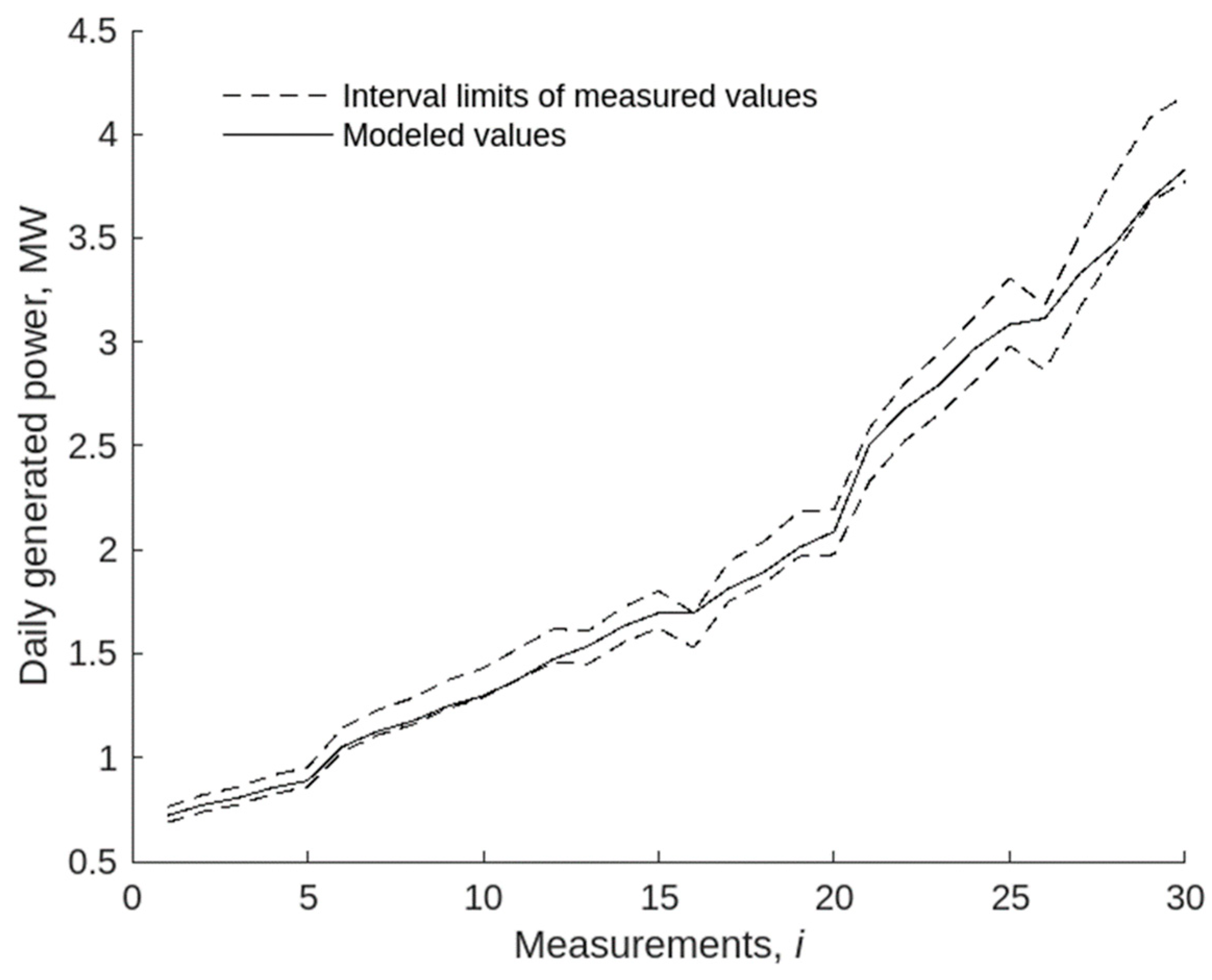
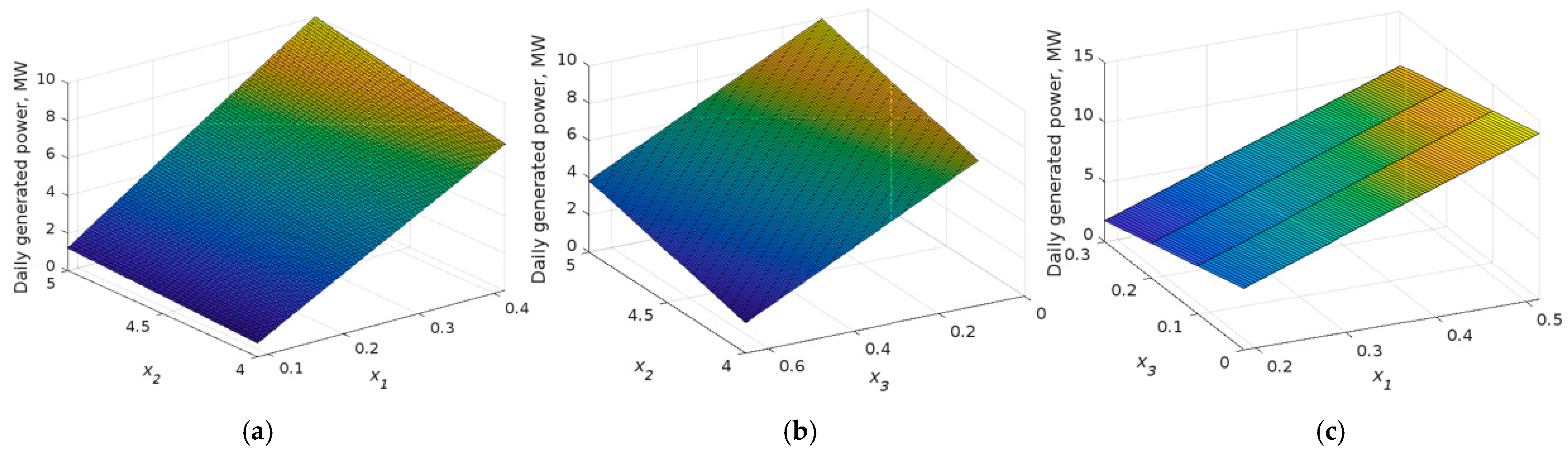
4. Results and Discussion

Using the derived mathematical model in (32), which describes the dependence of the generated electricity on water flow, head difference, and reactive power, we obtain Figure 4 and Figure 5. It is important to note that the obtained mathematical model fully corresponds to the physical processes of converting the gravitational force of water into electrical energy, taking into account the specifics of the hydro-technical and electrical equipment.

Figure 4 presents interval values corresponding to experimental data and modeled values based on the proposed model. The inclusion of the modeled values within the interval corridor demonstrates the adequacy and predefined accuracy of the obtained model, making it suitable for evaluating the efficiency of the hybrid station at the design stage.

Figure 5 presents three 3D graphs illustrating the dependence of daily generated power (MW) on two factors while keeping the third factor at a fixed average value. A detailed analysis of the surface slopes in the graphs reveals the dominant factor. Accordingly, the impact of daily water consumption is the most significant, as an increase leads to a substantial rise in generated power. Thus, accumulating additional water resources can effectively enhance power generation capacity.

The simulation results for the generated electricity based on the difference Equation (33) for one day of the summer and winter periods are shown in Figure 6a,b. The study utilizes proprietary software developed within the framework of the grant “Mathematical Tools and Software for the Prototype of a Biogas Plant with Increased Operational Efficiency”. The input parameters include experimental data for model construction and optimization algorithm tuning parameters.

Figure 6 displays the program windows with the results of model construction for dynamics based on the proposed methods, showing the modeled values that fall within the interval values of the experimental data, confirming the adequacy of the models, as well as the computed model parameters.

According to the proposed concept, all generated electricity is used to replenish hydro resources at the upper head level by pumping water from the lower head into a reservoir. Given that the SPP generates electricity only during daylight hours when solar radiation is available and is intended to compensate for peak loads in the grid, it is reasonable to convert this electricity into the gravitational potential energy of water resources. For this purpose, it is proposed to store hydro resources by pumping water from the lower head into a reservoir, which is currently located near the canal that supplies water to the SHPP. The schematic representation of the reservoir is shown in Figure 7.

At the moment, the volume of hydro resources in the reservoir is 40,010 m³. We will calculate the amount of water that can be pumped from the lower head to the reservoir using the daily electricity generation of the SPP. For the calculations, the winter and summer period graphs (Figure 6a,b) are used, which were constructed based on the SPP model in the form of a difference operator.

$$\underset{t_b}{\overset{t_a}{\int }}\left[\widehat{y}\right]dt=\sum _{k=t_b}^{t_a}\left[{\widehat{y}}_k\right].$$

(34)

Using the available data, we can calculate the volume of water that can be pumped from the lower head (from the canal behind the station) into the reservoir. When performing the calculation, it is essential to consider the actual amount of energy generated by the SPP. For this purpose, we use the following formula:

$$E_{efficient}={\eta }_{pump}·E,$$

(35)

where ${\eta }_{pump}=0.7$ (70%) is losses due to compression during hydro resource pumping.

$$m={\displaystyle \frac{E_{efficient}}{g·h}}.$$

(36)

From here, we determine the volume of water that can be pumped from the lower head to the reservoir:

$$\nu ={\displaystyle \frac{m}{\rho }},$$

(37)

where $\rho =1000$ kg/m³.

By substituting the simulation results based on the difference Equation (33) for the summer period into the equation for the summer period in Expression (34), then into (35), followed by (36) and (37), we obtain the volume of hydro resources that the system can accumulate during daylight hours. Considering the availability of 19,800 m³ of hydro resources that can be pumped into the reservoir within a day, it is necessary to raise the water level in the reservoir using a dam with a height of 0.74 m.

The pumping of hydro resources into the reservoir will be carried out using pumping equipment. Given the specifics of the combined operation of SHPP and SPP, particularly considering factors such as water flow rates, lift height, and operating duration, it is recommended to use multiple pumps to ensure the reliability and stability of the system’s operation.

Let us calculate how much energy the SHPP can generate from a single cycle of pumping water from the lower head to the reservoir.

For this, we will use the derived mathematical model in (32):

$$Y\left(X\right)=5.5254·{\left(19800·4\right)}^{0.9759}-11.3786·{\mathrm{x}}_3,$$

(38)

where ${\mathrm{x}}_1=\mathrm{19,800} \mathrm{m}³$ and ${\mathrm{x}}_2=4 \mathrm{m}.$

Thus, in one cycle (daily) of pumping hydro resources, the SHPP can generate an additional 183 kWh.

The performed calculations allow us to determine the potential for the integrated operation of the SHPP and SPP for electricity generation:

$${\eta }_{systems}={\displaystyle \frac{{{\rm E}}_2}{{{\rm E}}_1}}\cdot 100\%,$$

(39)

where ${{\rm E}}_2$ is the amount of electricity generated by the SHPP as a result of utilizing the pumped water in the reservoir and ${{\rm E}}_1$ is the amount of electricity generated by the SPP.

According to the results of experimental studies and modeling, as well as using Formula (39), the efficiency of the proposed system for the integrated operation of SHPP and SPP can reach 60%. The system ensures the maximum utilization of available resources, which contributes to stable electricity generation. This level of efficiency is due to the complementary interaction between these two types of stations and the optimization of their joint operation.

5. Conclusions

This article proposes a conceptual framework for an integrated system comprising two components: a small hydropower plant (SHPP) and a solar power plant (SPP). A key objective is to assess the potential of this system in terms of electricity generation. A methodology for evaluating the joint operation of a solar power plant and a small hydropower plant is proposed. The solar power plant generates electricity during daylight hours, which is used to power pumps. Electric pumps transfer water to an upper reservoir, from which it is subsequently utilized by the SHPP for electricity generation. Thus, the hydropower plant operates on the principle of a pumped storage hydropower system (PSH).

The methodology for assessing the integrated operation of both power plants is based on an interval model describing the dynamics of electricity generation by the photovoltaic system and a mathematical model that captures the relationship between the daily electricity generation of the SHPP and the influencing factors.

A novel hybrid method is proposed for the identification of both models. This method combines a metaheuristic algorithm for model structure synthesis, based on the behavioral model of a bee colony, with gradient-based methods for parameter estimation of the candidate models.

For the validation of the proposed concept, the “Topolky” SHPP, constructed on the Strypa River in the Ternopil region, was selected. This SHPP is equipped with two turbines connected to generators with capacities of 70 kW and 90 kW. It is proposed to install an additional SPP with a peak capacity of 100 kW adjacent to the existing SHPP. The installation consists of 193 JA Solar JAM72S30-550/MR solar panels, covering an area of 500 m². The system is proposed to be placed along the 100 m long and 5 m high channel that supplies hydro resources to the SHPP. To model the operation of the SPP, a study was conducted to examine the electricity generation potential during both the summer period (15 July) and the winter period (24 February). As a result, an interval model was developed to describe the daily electricity generation dynamics of the 100 kW peak capacity SPP. Based on this model, it was determined that, during the summer period, the SPP can generate more than 308 kWh per day and, during the winter period, this value decreases to approximately 200 kWh per day. The required volume of water to be pumped into the upper reservoir was calculated to be 19,800 m³ in summer, while, in the winter period, this volume is approximately 30% lower. These water volumes enable an increase in daily electricity production at the “Topolky” SHPP by up to 183 kW in summer. The calculations indicate that, during periods of reduced hydro resource availability (less than 86,000 m³ per day), the proposed approach would allow for a 25% increase in electricity generation at the SHPP.

Thus, the implementation of integrated systems, where a solar power plant and a hydropower plant operate jointly, is a viable and effective approach. This combination allows for maximizing the utilization of renewable energy sources and ensuring a stable electricity supply.

Key advantages are flexibility and stability. The system enables the use of renewable energy, such as solar power, for pumped storage hydropower. The proposed system enhances the stability of the energy network.

References

1. Adelekan, O.A.; Ilugbusi, B.S.; Adisa, O.; Obi, O.C.; Awonuga, K.F.; Asuzu, O.F.; Ndubuisi, N.L. Energy transition policies: A global review of shifts towards renewable sources. Eng. Sci. Technol. J. 2024, 5, 272–287. [Google Scholar] [CrossRef]
2. Maka, A.O.M.; Alabid, J.M. Solar energy technology and its roles in sustainable development. Clean Energy 2022, 6, 476–483. [Google Scholar] [CrossRef]
3. You, V.; Kakinaka, M. Modern and traditional renewable energy sources and CO2 emissions in emerging countries. Environ. Sci. Pollut. Res. 2022, 29, 17695–17708. [Google Scholar] [CrossRef] [PubMed]
4. Deshmukh, M.K.G.; Sameeroddin, M.; Abdul, D.; Sattar, M.A. Renewable energy in the 21st century: A review. Mater. Today Proc. 2023, 80, 1756–1759. [Google Scholar] [CrossRef]
5. Fernández, D.G.; Fajardo-Moreno, W.; Moreno-Monsalve, N. Analysis of Non-Conventional Renewable Energy Sources Projects in Colombia. In Proceedings of the 2023 IEEE Colombian Conference on Communications and Computing (COLCOM), Bogota, Colombia, 26–28 July 2023; pp. 1–4. [Google Scholar]
6. Büyüközkan, G.; Karabulut, Y.; Mukul, E. A novel renewable energy selection model for United Nations’ sustainable development goals. Energy 2018, 165, 290–302. [Google Scholar] [CrossRef]
7. Yousef, L.A.; Yousef, H.; Rocha-Meneses, L. Artificial Intelligence for Management of Variable Renewable Energy Systems: A Review of Current Status and Future Directions. Energies 2023, 16, 8057. [Google Scholar] [CrossRef]
8. Koshlak, H. A Review of Earth-Air Heat Exchangers: From Fundamental Principles to Hybrid Systems with Renewable Energy Integration. Energies 2025, 18, 1017. [Google Scholar] [CrossRef]
9. Ahmed, B.; Al Mubarak, M.; Khouj, M. Renewable Technologies: Solar Power and Wind Power Energy Utilization—Advantages and Disadvantages. In Technological Sustainability and Business Competitive Advantage. Internet of Things; Al Mubarak, M., Hamdan, A., Eds.; Springer: Cham, Switzerland, 2023. [Google Scholar]
10. Rahman, A.; Farrok, O.; Haque, M.M. Environmental impact of renewable energy source based electrical power plants: Solar, wind, hydroelectric, biomass, geothermal, tidal, ocean, and osmotic. Renew. Sustain. Energy Rev. 2022, 161, 112279. [Google Scholar] [CrossRef]
11. Idoko, I.P.; Ayodele, T.R.; Abolarin, S.M.; Ewim, D.R.E. Maximizing the cost effectiveness of electric power generation through the integration of distributed generators: Wind, hydro and solar power. Bull. Natl. Res. Cent. 2023, 47, 166. [Google Scholar] [CrossRef]
12. Medina, J.C.L.; Concepción, V.H.; Zerpa, F.A.L.; Pino, C.A.M. Gran Canaria energy system: Integration of the chira-soria pumped hydroelectric power plant and analysis of weekly daily demand patterns for the year 2023. Renew. Energy 2024, 232, 121128. [Google Scholar] [CrossRef]
13. Jurasz, J.; Tomczyk, P.; Bochenek, B.; Kuriqi, A.; Kasiulis, E.; Chen, D.; Ming, B. Solar-hydro cable pooling–Utilizing the untapped potential of existing grid infrastructure. Energy Convers. Manag. 2024, 306, 118307. [Google Scholar] [CrossRef]
14. Fan, J.L.; Huang, X.; Shi, J.; Li, K.; Cai, J.; Zhang, X. Complementary potential of wind-solar-hydro power in Chinese provinces: Based on a high temporal resolution multi-objective optimization model. Renew. Sustain. Energy Rev. 2023, 184, 113566. [Google Scholar] [CrossRef]
15. Nasir, J.; Javed, A.; Ali, M.; Ullah, K.; Kazmi, S.A.A. Sustainable and cost-effective hybrid energy solution for arid regions: Floating solar photovoltaic with integrated pumped storage and conventional hydropower. J. Energy Storage 2023, 74, 109417. [Google Scholar] [CrossRef]
16. Zeidan, M.; Al-soud, M.; Dmour, M.; Alakayleh, Z.; Al-qawabah, S. Integrating a Solar PV System with Pumped Hydroelectric Storage at the Mutah University of Jordan. Energies 2023, 16, 5769. [Google Scholar] [CrossRef]
17. Mamatha, G.; Verma, A.; Kulkarni, P.S. Proposing a Hybrid Solar Electrification for Already Existing Hydropower Plant. In Proceedings of the 2024 IEEE Students Conference on Engineering and Systems (SCES), Prayagraj, India, 21–23 June 2024; pp. 1–6. [Google Scholar]
18. Lima, G.M.; Belchior, F.N.; Villena, J.E.N.; Domingos, J.L.; Freitas, M.A.V.; Hunt, J.D. Hybrid electrical energy generation from hydropower, solar photovoltaic and hydrogen. Int. J. Hydrogen Energy 2024, 53, 602–612. [Google Scholar] [CrossRef]
19. Dyvak, M.; Melnyk, A.; Manzhula, V.; Petryshyn, N.; Brukhanskyi, R.; Tymets, V. The Approach to Modelling the Joint Operation of a Solar Power Plant and a Small Hydropower Plant. In Proceedings of the 2024 IEEE 17th International Conference on Advanced Trends in Radioelectronics, Telecommunications and Computer Engineering (TCSET 2024), Lviv, Ukraine, 8–12 October 2024; pp. 217–222. [Google Scholar]
20. Dyvak, M. Parameters Identification Method of Interval Discrete Dynamic Models of Air Pollution Based on Artificial Bee Colony Algorithm. In Proceedings of the 2020 10th International Conference on Advanced Computer Information Technologies (ACIT), Deggendorf, Germany, 16–18 September 2020; pp. 130–135. [Google Scholar]
21. Dyvak, M.; Pukas, A.; Oliynyk, I.; Melnyk, A. Selection the “Saturated” Block from Interval System of Linear Algebraic Equations for Recurrent Laryngeal Nerve Identification. In Proceedings of the 2018 IEEE Second International Conference on Data Stream Mining & Processing (DSMP), Lviv, Ukraine, 21–25 August 2018; pp. 444–448. [Google Scholar]
22. Li, Y.; Ming, B.; Huang, Q.; Wang, Y.; Liu, P.; Guo, P. Identifying effective operating rules for large hydro–solar–wind hybrid systems based on an implicit stochastic optimization framework. Energy 2022, 245, 123260. [Google Scholar] [CrossRef]
23. Gonzalez-Gonzalez, J.J.; Arenas-López, J.P.; Badaoui, M. Advancing towards zero emissions: Integrating floating photovoltaic systems in hydroelectric power plant reservoirs. Results Eng. 2024, 23, 102742. [Google Scholar] [CrossRef]
24. Caldeira, M.J.V.; Ferraz, G.M.F.; Santos, I.F.S.D.; Filho, G.L.T.; Barros, R.M. Using solar energy for complementary energy generation and water level recovery in Brazilian hybrid hydroelectricity: An energy and economic study. Renew. Energy 2023, 218, 119287. [Google Scholar] [CrossRef]
25. Glasnovic, Z.; Margeta, J. The features of sustainable Solar Hydroelectric Power Plant. Renew. Energy 2009, 34, 1742–1751. [Google Scholar] [CrossRef]
26. Rauf, H.; Gull, M.S.; Arshad, N. Complementing hydroelectric power with floating solar PV for daytime peak electricity demand. Renew. Energy 2020, 162, 1227–1242. [Google Scholar] [CrossRef]
27. Hoseinzadeh, S.; Ghasemi, M.H.; Heyns, S. Application of hybrid systems in solution of low power generation at hot seasons for micro hydro systems. Renew. Energy 2020, 160, 323–332. [Google Scholar] [CrossRef]
28. Kougias, I.; Szabó, S.; Monforti-Ferrario, F.; Huld, T.; Bódis, K. A methodology for optimization of the complementarity between small-hydropower plants and solar PV systems. Renew. Energy 2016, 87, 1023–1030. [Google Scholar] [CrossRef]
29. Silvério, N.M.; Barros, R.M.; Filho, G.L.T.; Redón-Santafé, M.; Santos, I.F.S.D.; de Mello Valério, V.E. Use of floating PV plants for coordinated operation with hydropower plants: Case study of the hydroelectric plants of the São Francisco River basin. Energy Convers. Manag. 2018, 171, 339–349. [Google Scholar] [CrossRef]
30. Abdelhafidi, N.; Yılmaz, İ.H.; Bachari, N.E.I. An innovative dynamic model for an integrated solar combined cycle power plant under off-design conditions. Energy Convers. Manag. 2020, 220, 113066. [Google Scholar] [CrossRef]
31. Bhayo, B.A.; Al-Kayiem, H.H.; Gilani, S.I.U.; Ismail, F.B. Power management optimization of hybrid solar photovoltaic-battery integrated with pumped-hydro-storage system for standalone electricity generation. Energy Convers. Manag. 2020, 215, 112942. [Google Scholar] [CrossRef]
32. Wang, Z.; Fang, G.; Wen, X.; Tan, Q.; Zhang, P.; Liu, Z. Coordinated operation of conventional hydropower plants as hybrid pumped storage hydropower with wind and photovoltaic plants. Energy Convers. Manag. 2023, 277, 116654. [Google Scholar] [CrossRef]
33. Temraz, A.; Alobaid, F.; Link, J.; Elweteedy, A.; Epple, B. Development and Validation of a Dynamic Simulation Model for an Integrated Solar Combined Cycle Power Plant. Energies 2021, 14, 3304. [Google Scholar] [CrossRef]
34. Zhou, Y.; Chang, F.-J.; Chang, L.-C.; Lee, W.-D.; Huang, A.; Xu, C.-Y.; Guo, S. An advanced complementary scheme of floating photovoltaic and hydropower generation flourishing water-food-energy nexus synergies. Appl. Energy 2020, 275, 115389. [Google Scholar] [CrossRef]
35. Zhang, Y.; Ma, C.; Lian, J.; Pang, X.; Qiao, Y.; Chaima, E. Optimal photovoltaic capacity of large-scale hydro-photovoltaic complementary systems considering electricity delivery demand and reservoir characteristics. Energy Convers. Manag. 2019, 195, 597–608. [Google Scholar] [CrossRef]
36. Sachenko, A.; Kochan, V.; Turchenko, V.; Tymchyshyn, V.; Vasylkiv, N. Intelligent nodes for distributed sensor network. In Proceedings of the 16th IEEE Instrumentation and Measurement Technology Conference (Cat. No.99CH36309) (IMTC/99), Venice, Italy, 24–26 May 1999; Volume 3, pp. 1479–1484. [Google Scholar]
37. Lytvyn, V.; Vysotska, V.; Pukach, P.; Nytrebych, Z.; Demkiv, I.; Senyk, A.; Malanchuk, O.; Sachenko, S.; Kovalchuk, R.; Huzyk, N. Analysis of the developed quantitative method for automatic attribution of scientific and technical text content written in Ukrainian. East.-Eur. J. Enterp. Technol. 2018, 6, 19–31. [Google Scholar] [CrossRef]
38. Li, H.; Liu, P.; Guo, S.; Ming, B.; Cheng, L.; Yang, Z. Long-term complementary operation of a large-scale hydro-photovoltaic hybrid power plant using explicit stochastic optimization. Appl. Energy 2019, 238, 863–875. [Google Scholar] [CrossRef]
39. León Gómez, J.C.; De León Aldaco, S.E.; Aguayo Alquicira, J. A Review of Hybrid Renewable Energy Systems: Architectures, Battery Systems, and Optimization Techniques. Eng 2023, 4, 1446–1467. [Google Scholar] [CrossRef]
40. Bartolucci, L.; Cordiner, S.; Mulone, V.; Rocco, V.; Rossi, J.L. Hybrid renewable energy systems for renewable integration in microgrids: Influence of sizing on performance. Energy 2018, 152, 744–758. [Google Scholar] [CrossRef]
41. Hassan, Q. Optimisation of solar-hydrogen power system for household applications. Int. J. Hydrogen Energy 2020, 45, 33111–33127. [Google Scholar] [CrossRef]
42. Javed, M.S.; Zhong, D.; Ma, T.; Song, A.; Ahmed, S. Hybrid pumped hydro and battery storage for renewable energy based power supply system. Appl. Energy 2020, 257, 114026. [Google Scholar] [CrossRef]
43. Calise, F.; Dentice d’Accadia, M.; Libertini, L.; Vicidomini, M. Thermoeconomic analysis of an integrated solar combined cycle power plant. Energy Convers. Manag. 2018, 171, 1038–1051. [Google Scholar] [CrossRef]
44. Fedor, P.; Perdukova, D.; Bernat, P.; Štěpanec, L.; Fedák, V. Modeling of Electromagnetic Phenomena in Small Hydroelectric Plants. In Proceedings of the 2023 International Conference on Electrical Drives and Power Electronics (EDPE), The High Tatras, Slovakia, 25–27 September 2023. [Google Scholar]
45. Dyvak, M.; Spivak, I.; Melnyk, A.; Manzhula, V.; Dyvak, T.; Rot, A.; Hernes, M. Modeling Based on the Analysis of Interval Data of Atmospheric Air Pollution Processes with Nitrogen Dioxide due to the Spread of Vehicle Exhaust Gases. Sustainability 2023, 15, 2163. [Google Scholar] [CrossRef]
46. Dyvak, M.; Stakhiv, P.; Pukas, A. Algorithms of parallel calculations in task of tolerance ellipsoidal estimation of interval model parameters. Bull. Pol. Acad. Sci. 2012, 60, 159–164. [Google Scholar] [CrossRef]
47. Ocheretnyuk, N.; Voytyuk, I.; Dyvak, M.; Martsenyuk, Y. Features of structure identification the macromodels for nonstationary fields of air pollutions from vehicles. Proceedings of International Conference on Modern Problem of Radio Engineering, Telecommunications and Computer Science, Lviv, Ukraine, 21–24 February 2012; p. 444. [Google Scholar]
48. Darmorost, I.; Dyvak, M.; Porplytsya, N.; Shynkaryk, T.; Martsenyuk, Y.; Brych, V. Convergence Estimation of a Structure Identification Method for Discrete Interval Models of Atmospheric Pollution by Nitrogen Dioxide. In Proceedings of the 2019 9th International Conference on Advanced Computer Information Technologies (ACIT), Ceske Budejovice, Czech Republic, 5–7 June 2019; pp. 117–120. [Google Scholar]
49. Mykola, D.; Krzysztof, G.; Janusz, Z.; Natalia, P.; Jacek, D.; Ewa, K. Mathematical Model of Dynamics of Generated Electric Power by Photovoltaic Installation Taking into Account a Seasonality Factor. In Proceedings of the 2020 10th International Conference on Advanced Computer Information Technologies (ACIT), Deggendorf, Germany, 16–18 September 2020. [Google Scholar]
Figure 1. Illustration of the combined operation of a small hydropower plant and a solar power plant.
Energies 18 02351 g001
Figure 2. Illustration of the operation of a SHPP “Topolky”: (a) SHPP building with a sluice for water supply to the turbine, (b) hydraulic units of the SHPP.
Energies 18 02351 g002
Figure 3. (a) Map of the area of SHPP “Topolky” in the city of Buchach; (b) solar panels installed in the 6th academic building of WUNU.
Energies 18 02351 g003
Figure 4. Graphs of the interval values of the daily generated electricity and the simulated values.
Energies 18 02351 g004
Figure 5. Dependence of the daily generated electricity: (a) on water flow (x1) and head (x2); (b) on head (x2) and reactive power (x3); (c) on water flow (x1) and reactive power (x3).
Energies 18 02351 g005
Figure 6. Daily dynamics of the generated power by the studied photovoltaic installation for different seasons using Model (33): (a)—as of 15 July, (b)—as of 24 December.
Energies 18 02351 g006
Figure 7. Graphical representation of the proposed tank for the station.
Energies 18 02351 g007