
Optimal Siting and Sizing of Battery Energy Storage System in Distribution System in View of Resource Uncertainty


Abstract
1. Introduction
- Proposal of a multiple-objective function (MOF) based on minimizing the APL and PSI and maximizing the VSI for the OPSBESS.
- Incorporation of uncertainties in the resource for the OPSBESS using probabilistic and PMR approaches for MBRDSs.
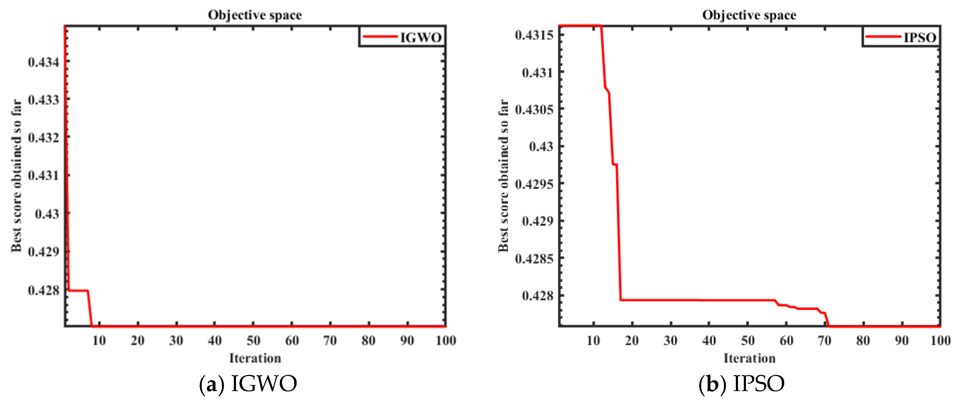
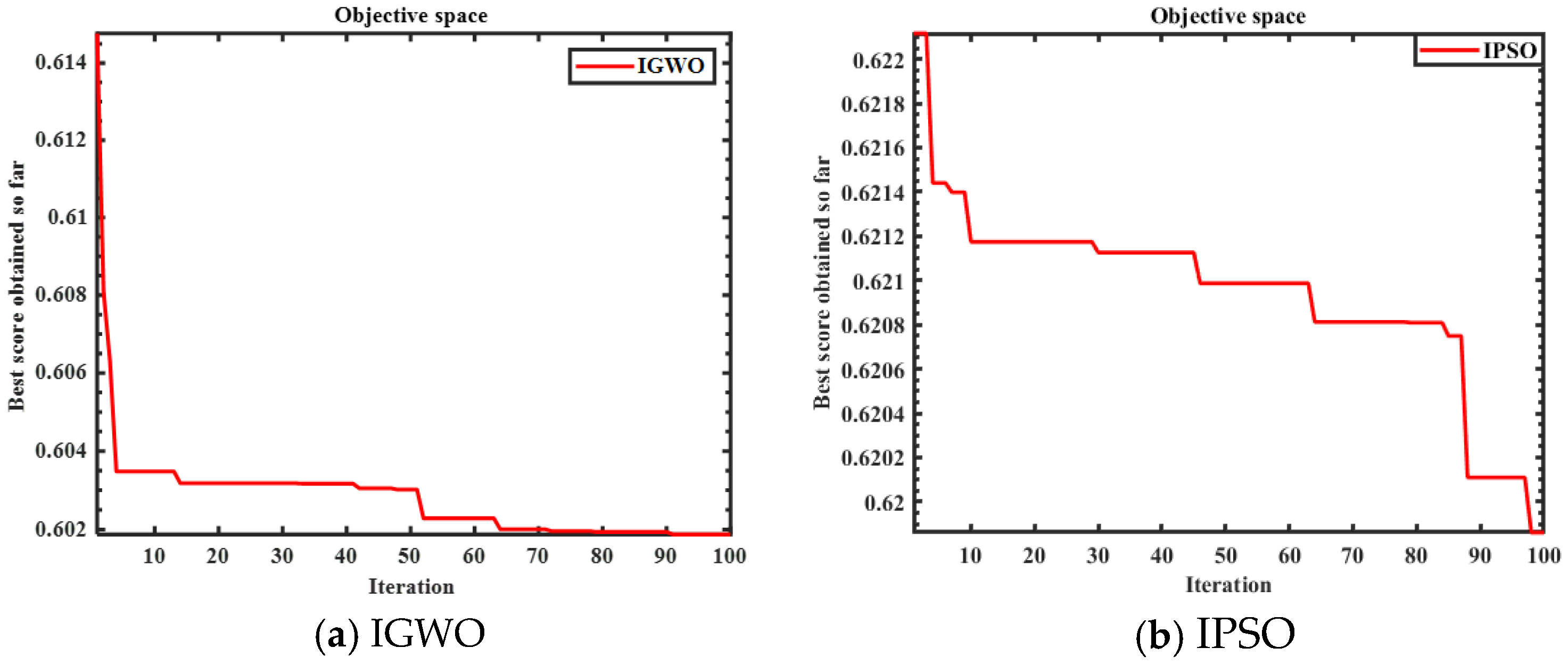
- Analysis of simultaneously and sequentially distributed BESS placement to understand the system behavior using IGWO and TOPSIS (IGT). The results are validated using Improved Particle Swarm Optimization–TOPSIS (IPT) techniques.
2. Grid-Connected PV-BES System
2.1. Solar PV System
2.1.1. Deterministic Approach
2.1.2. Probabilistic Approach
- s(t): solar irradiance (W/m2) at ‘t’;
- Ppv(t): total power output of PV panels at ‘t’(W);
- ηPV: efficiency of PV panel (%);
- A: area of PV panel (m2).
2.1.3. Polynomial Multiple Regression Approach (PMRA)
2.2. Load
2.3. BESS
- EPV(t): energy generated by the solar PV at instant t (kWh);
- Eload(t): energy required by the load at instant t (kWh);
- EBESS(t): energy stored by the BESS at instant t (kWh);
- ρ: self-discharge rate of the BESS;
- ηBESS: charging and discharging efficiencies of the BESS;
- ηinv: efficiency of the inverter.
3. Multi-Objective Problem Formulation and Constraints
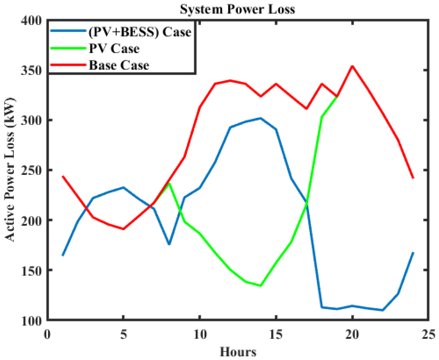
3.1. Minimization of APL (F1)
- N: number of buses in the system;
- Rij: resistance of branch between bus i and bus j (Ω);
- Pi: injected active power at the ith bus (watt);
- Pj: injected active power at the jth bus (watt);
- Qi: injected reactive power at the ith bus (VAR);
- Qj: injected reactive power at the jth bus (VAR);
- Vi: voltage magnitude at sending end voltage at the ith bus (volts);
- Vj: voltage magnitude at receiving end voltage at the jth bus (volts);
- δi: phase angle at the ith bus (radians);
- δj: phase angle at the jth bus (radians).
3.2. Minimization of PSI (F2)
- Rij: resistance of branch between bus i and bus j (Ω);
- PL: active power at the load bus (watt);
- PG: injected active power into the system (watt);
- Vi: sending end voltage (volts);
- θ: angle of line impedance (radians);
- δ: phase angle (radians).
3.3. Maximization of VSI (F3)
- VSIi: Voltage Stability Index of bus ‘j’;
- Pj: (sum of the active power loads of all the buses beyond bus j) + (active power load of bus j itself) + (sum of the Active Power Losses of all the branches beyond bus j) (watt);
- Qj: (sum of the reactive power loads of all the buses beyond bus j) + (reactive power load of bus j itself) + (sum of the reactive power losses of all the branches beyond bus j) (VAR);
- Rij: resistance of the branch connecting bus i and bus j (Ω);
- Xij: reactance of the branch connecting bus i and bus j (Ω);
- Vi: sending end voltage (volts).
3.4. Multi-Objective Problem Formulation
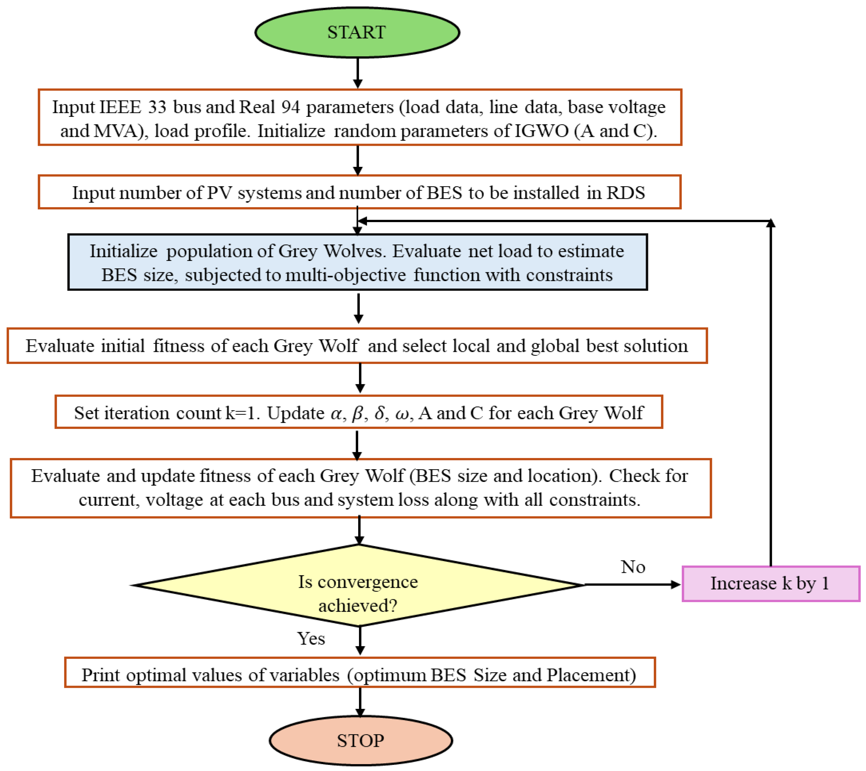
4. IGWO for OPSBESS
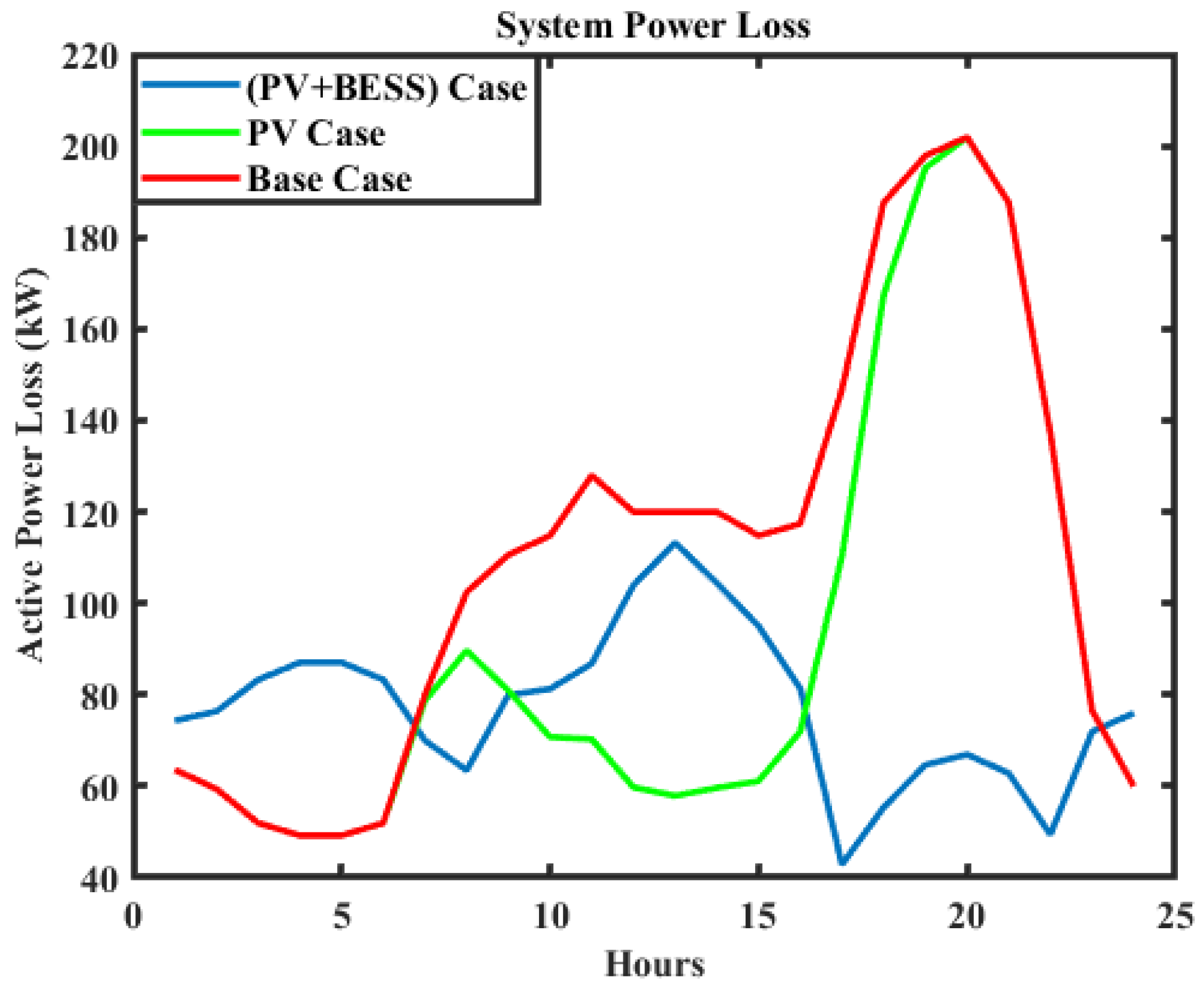
5. Results and Discussion
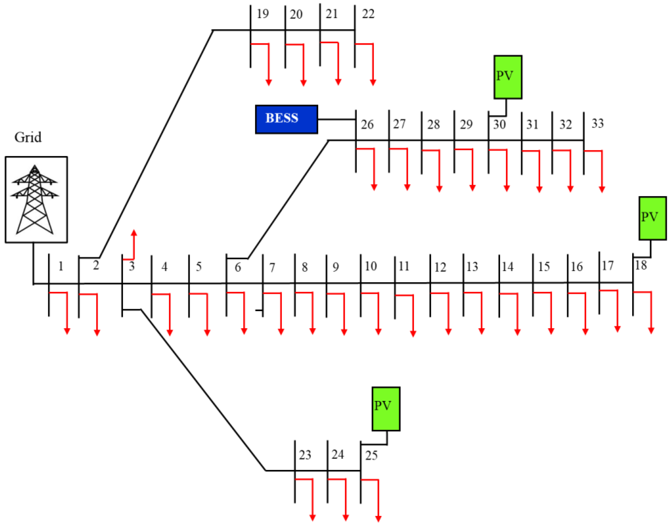
5.1. IEEE 33-Bus RDS
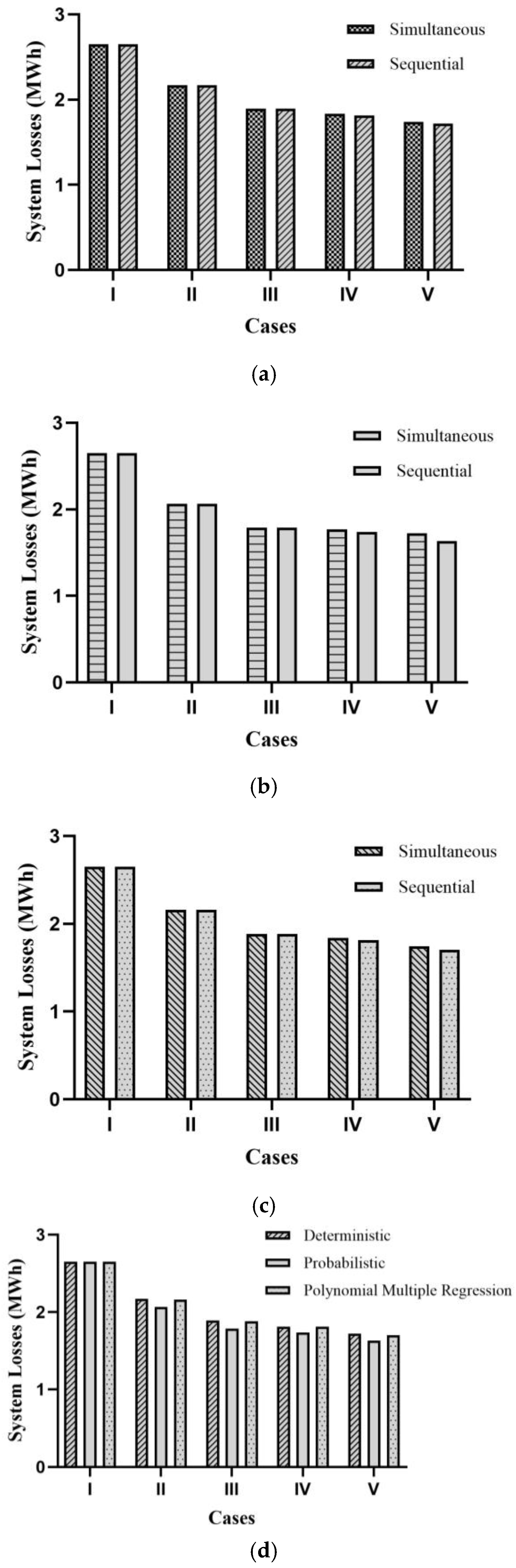
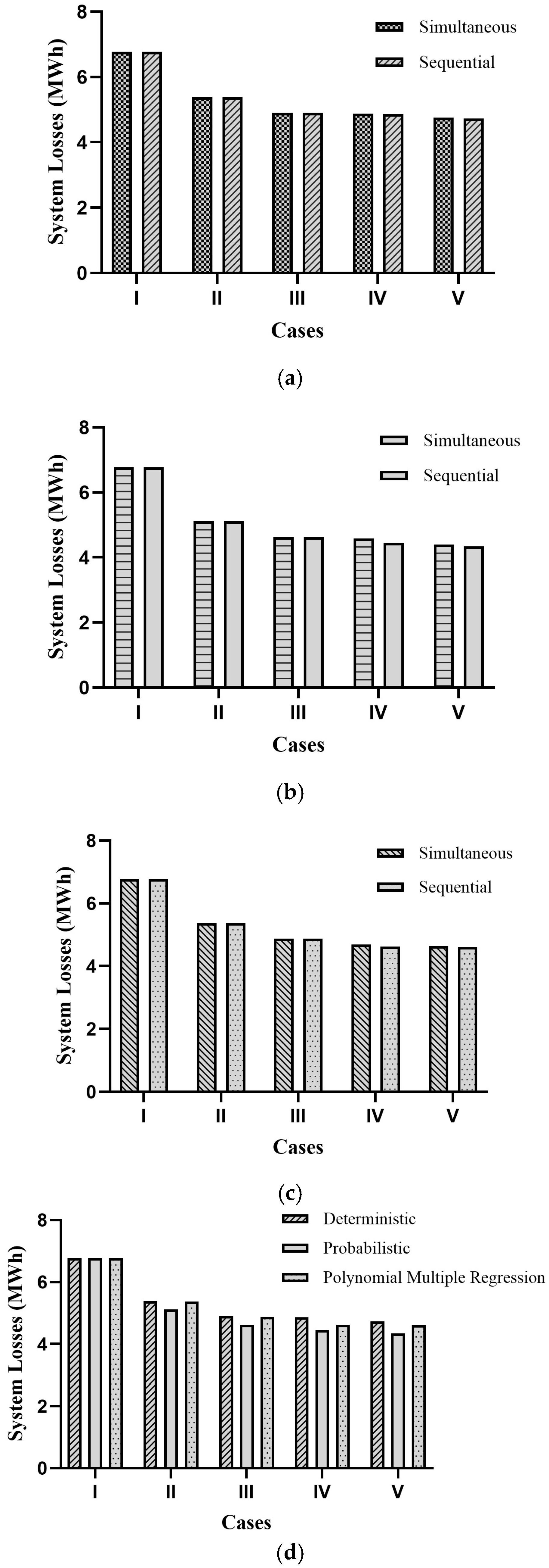
5.2. Analysis of MBRDS Using Simultaneous and Sequential BESS Placements
5.2.1. Simultaneous BESS Placements
5.2.2. Sequential BESS Placements
5.3. Analysis of System Parameters for Probabilistic Approach (Beta PDF) for MBRDS
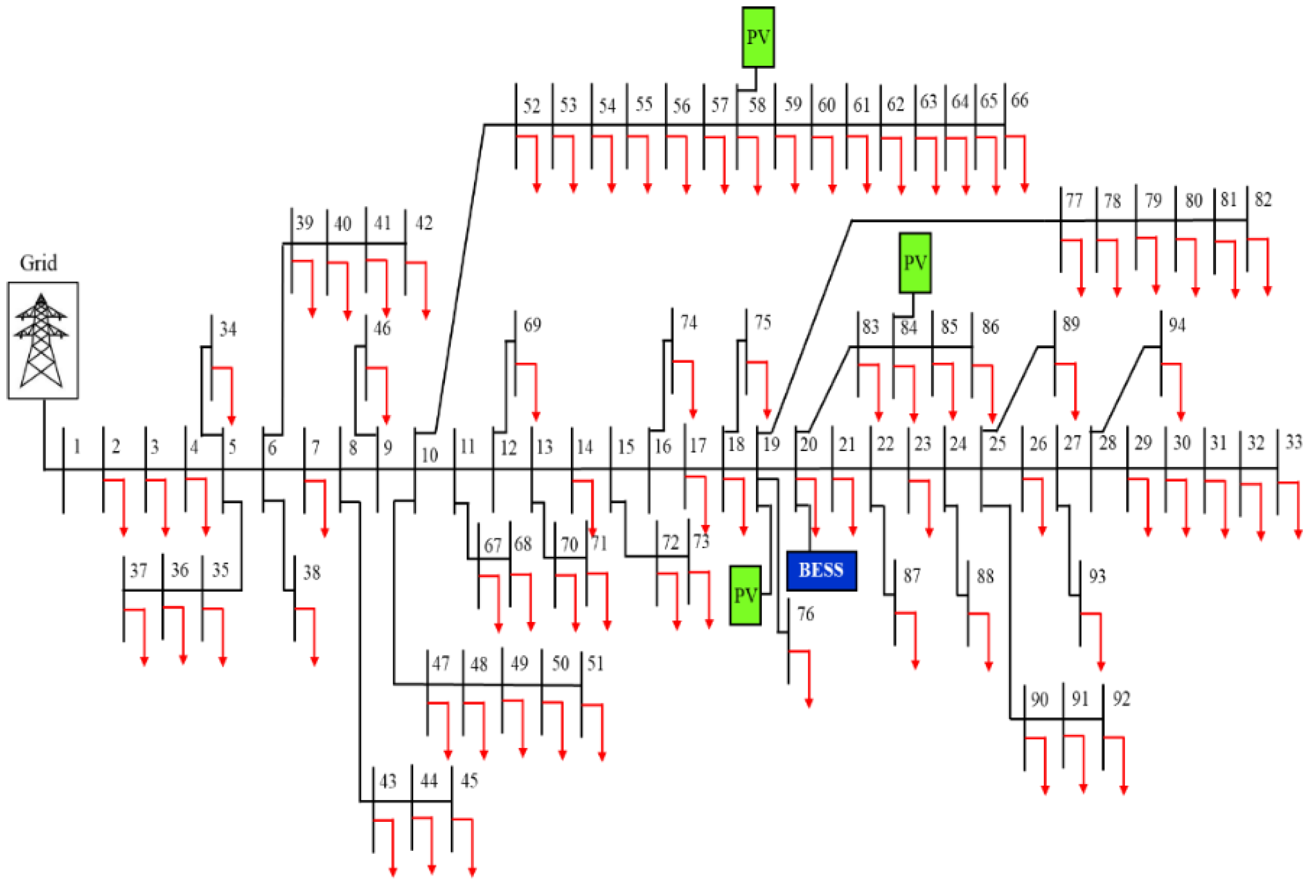
5.4. Real 94-Bus Portuguese RDS
5.4.1. Analysis of MRBPRDS Using Simultaneous and Sequential BESS Placements
5.4.2. Analysis of System Parameters for Probabilistic (Beta PDF) Approach for Real 94-Bus Portuguese RDS
6. Conclusions
Author Contributions
Funding
Data Availability Statement
Conflicts of Interest
Abbreviations
| Nomenclature | |
| PRS | Rated PV power (kW) |
| s | Solar irradiance (kW/m2) |
| RSRS | Solar radiation with the standard environment (kW/m2) |
| RCR | Certain solar irradiance (kW/m2) |
| Ppv-single | Power rating of single PV panel (kW) |
| NPV | Number of PV panels |
| Ppv | Total power output of all PV panels (kW) |
| Γ | Gamma function |
| α, β | Shape parameters of the β-PDF |
| μ and σ | Mean and standard deviation |
| p(s) | Probability of solar irradiance (W/m2) |
| t | Particular instant |
| TNOCT | Temperature at Nominal Operating Cell Temperature (°C) |
| Ta | Ambient temperature (°C) |
| Tc | Cell temperature (°C) |
| VMPP | Voltage at Maximum Power Point (V) |
| IMPP | Current at Maximum Power Point (A) |
| KV | Voltage temperature coefficient (V/°C) |
| Ki | Current temperature coefficient (A/°C) |
| VNET | Net voltage (V) |
| VOC | Open-Circuit Voltage (V) |
| INET | Net current (A) |
| ISC | Short-Circuit Current (A) |
| Fill Factor | Efficiency of PV panel (%) |
| A | Area of PV panel (m2) |
| ηPV | Efficiency of PV panel (%) |
| ρ | Self-discharge rate of BESS |
| EPV(t) | Energy generated by PV (kWh) |
| Eload(t) | Energy required by load (kWh) |
| EBESS(t) | Energy stored in battery/BESS (kWh) |
| ɳBESS | Efficiency of BESS (%) |
| ɳinv | Efficiency of inverter (%) |
| N | Number of buses |
| Pi and Qi | Active (W) and reactive (VAR) power injections at the ith bus |
| Pj and Qj | Active (W) and reactive (VAR) power injections at the jth bus |
| Rij and Xij | Resistance and reactance of the branch connecting ith and jth buses (Ω) |
| Vi and δi | Voltage magnitude (volts) and angle (radians) at the ith bus |
| Vj and δj | Voltage magnitude (volts) and angle (radians) at the jth bus |
| Yij and θij | Elements of Y-bus matrix (siemens) and impedance angles (radians) |
| δ | Phase angle (radians) |
| PL | Active power at load bus (W) |
| PG | Generated active power of the system (W) |
| Abbreviations | Full Form |
| DGs | Distributed Generations |
| RDSs | Radial Distribution Systems |
| BES | Battery Energy Storage |
| PMR | Polynomial Multiple Regression |
| RERs | Renewable Energy Resources |
| PV | Photovoltaic |
| BESS | Battery Energy Storage System |
| OPSBESS | Optimal Placement and Sizing of BESS |
| PSI | Power Stability Index |
| APL | Active Power Loss |
| VSI | Voltage Stability Index |
| WSM | Weighted Sum Method |
| IGWO | Improved Grey Wolf Optimization |
| IPSO | Improved Particle Swarm Optimization |
| TOPSIS | Technique for Order of Preference by Similarity to the Ideal Solution |
| β-PDF | Beta Probability Density Function |
| MBRDS | Modified IEEE 33-bus Radial Distribution System |
| MRBPRDS | Modified real 94-bus Portuguese Radial Distribution System |
| MOF | Multi-objective function |
| PMRA | Polynomial Multiple Regression Approach |
| SOC | State of Charge |
| DSs | Distribution Systems |
| MCDM | Multi-Criteria Decision-Making |
Appendix A
A.1. Comparison of System Parameters for Deterministic and Polynomial Multiple Regression (PMR) Approaches for Modified IEEE 33-Bus RDS (MBRDS)

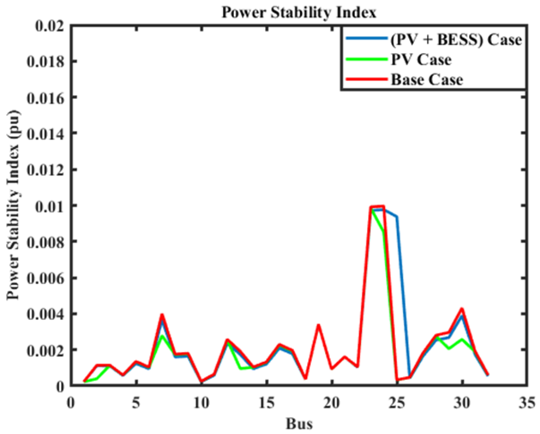
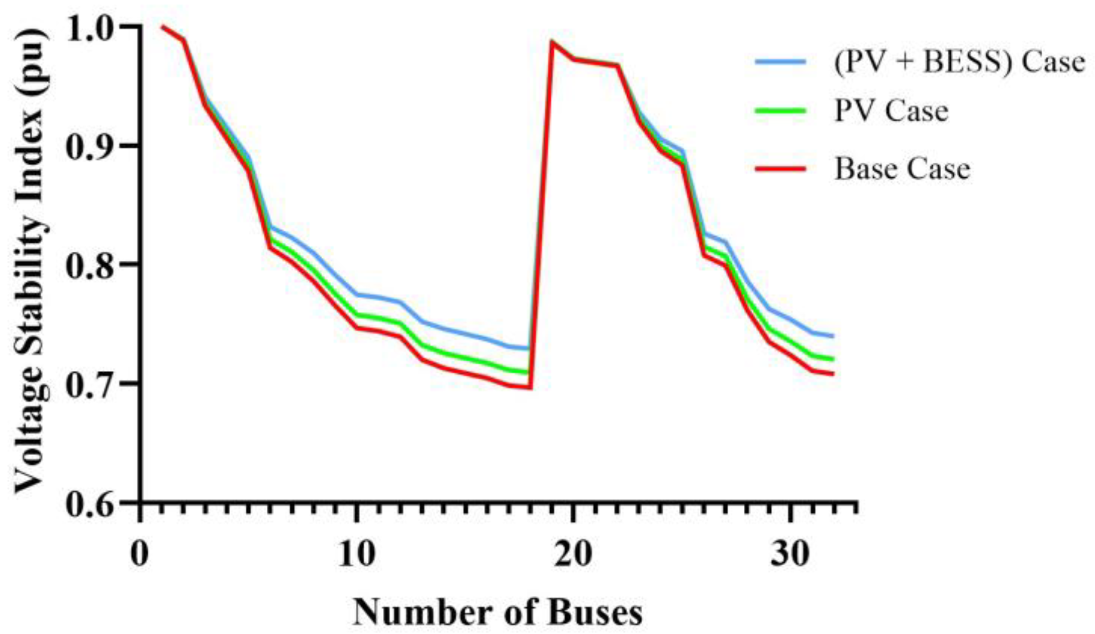
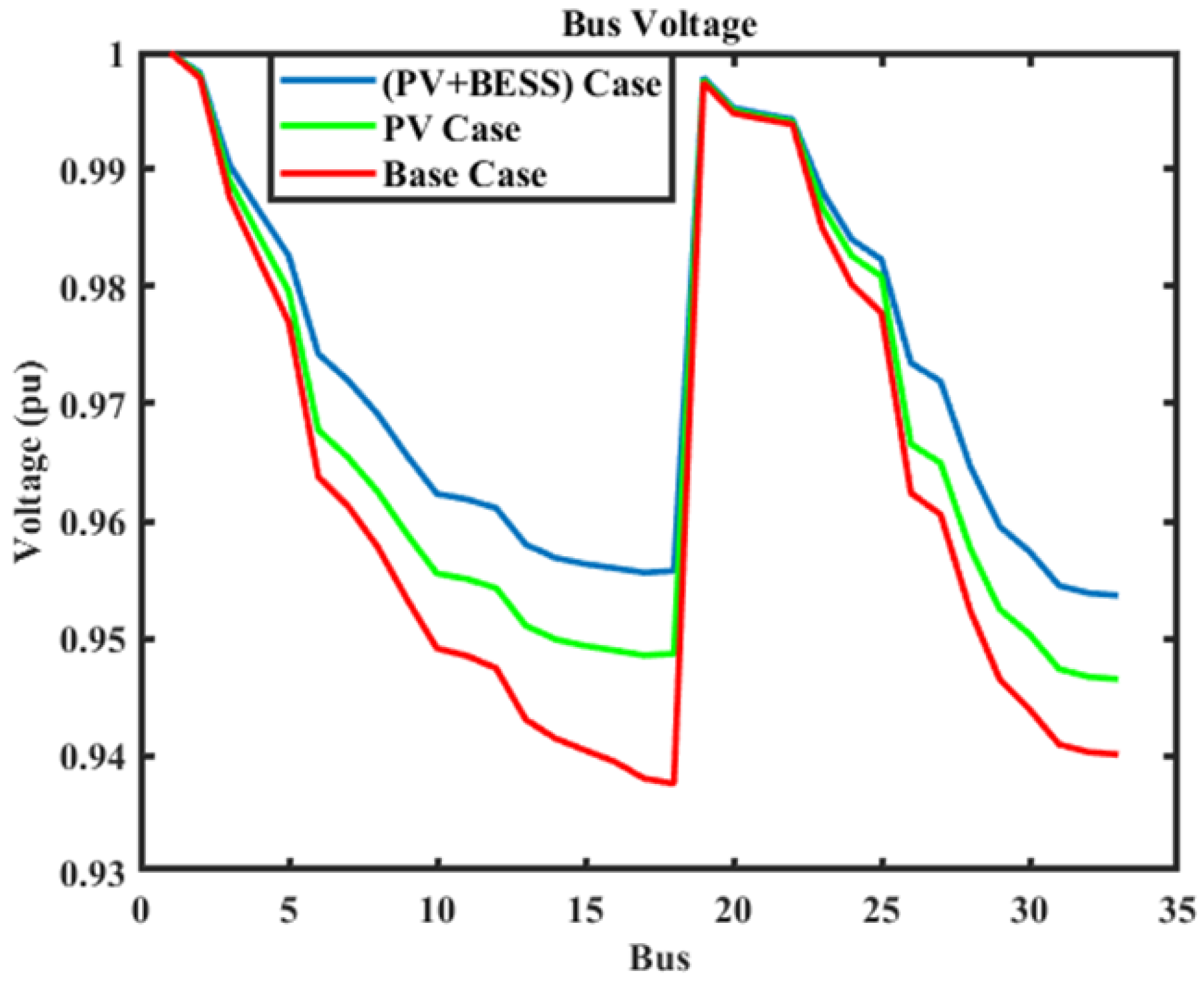
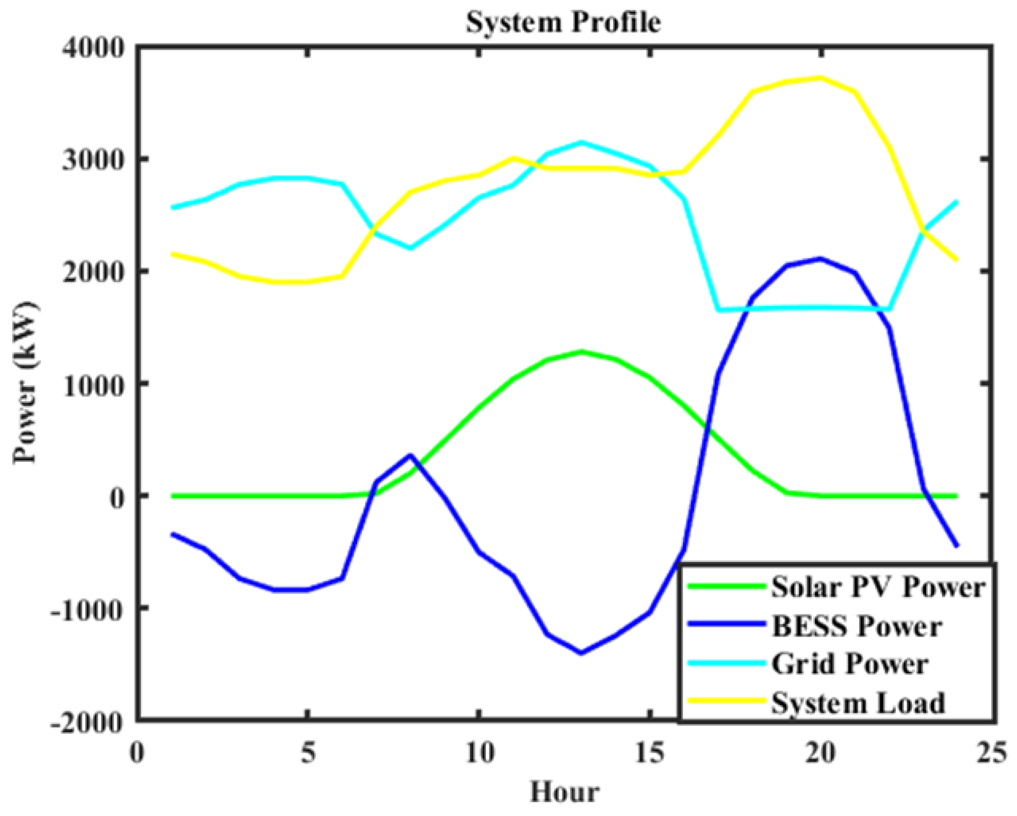
| Parameters | Deterministic Approach (BESS Size = 2.3 MW) | PMR Approach (BESS Size = 2.4 MW) |
|---|---|---|
| PSI | 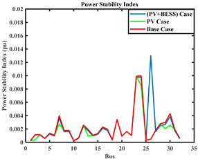 | 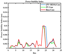 |
| VSI | 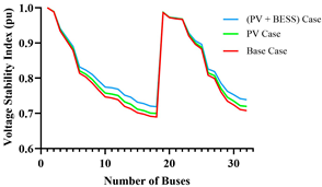 | 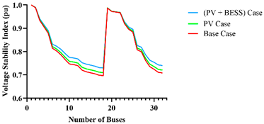 |
| Bus voltage profile |  |  |
| System profile |  |  |
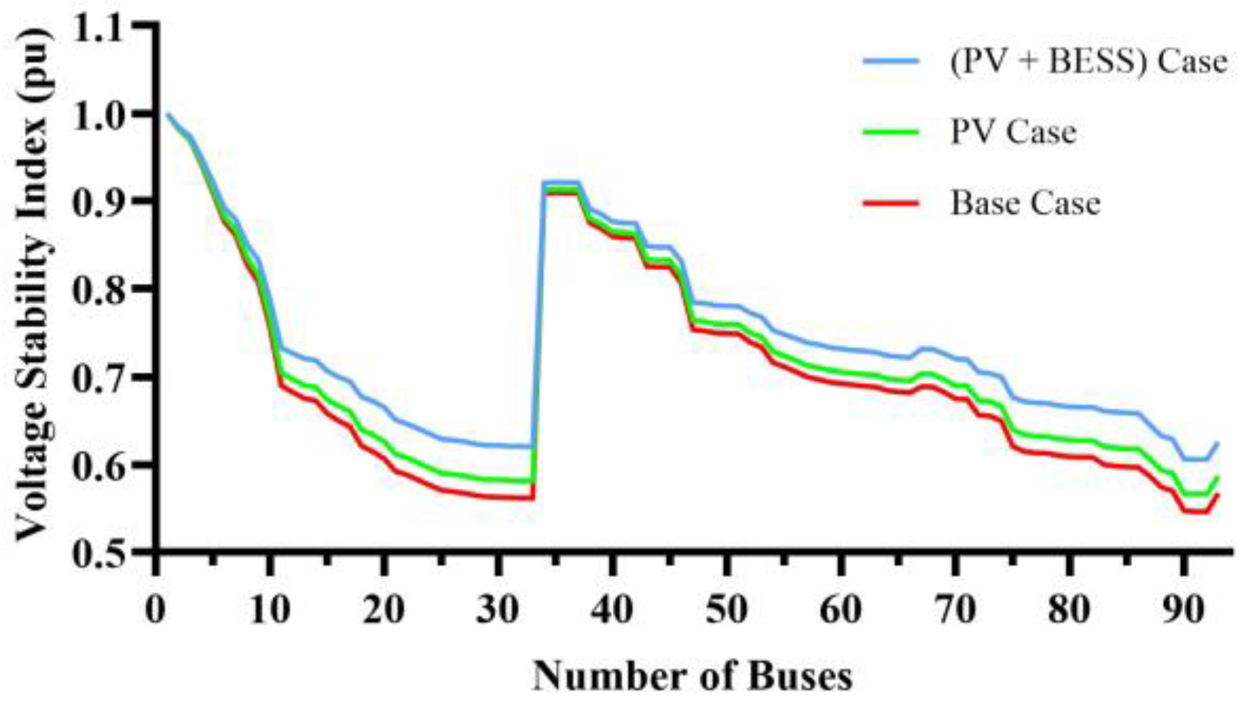
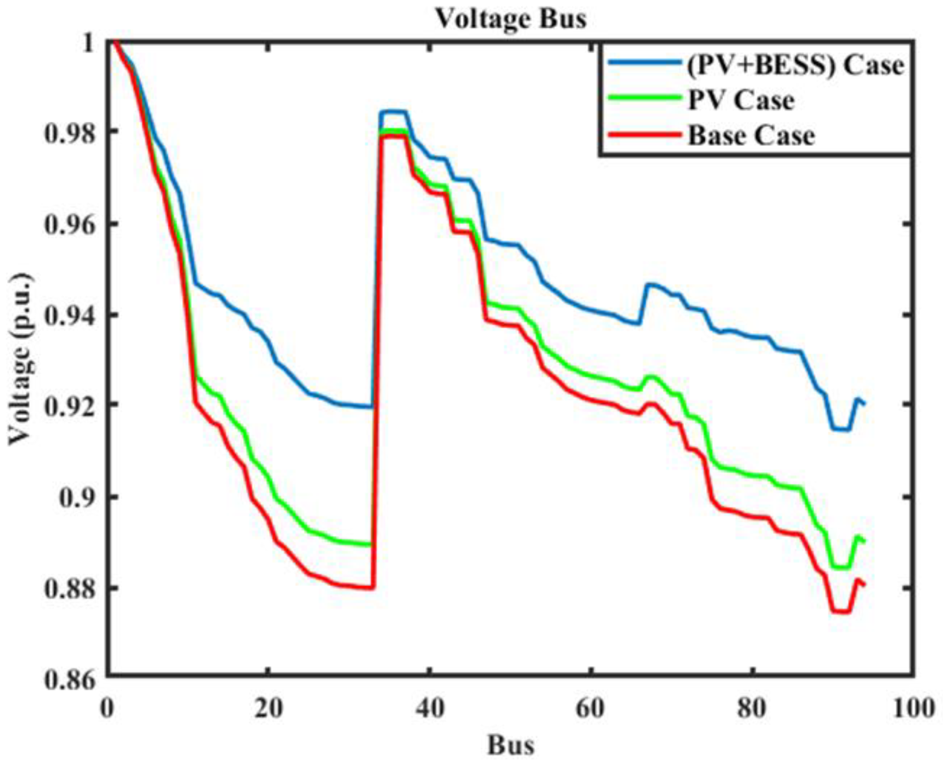
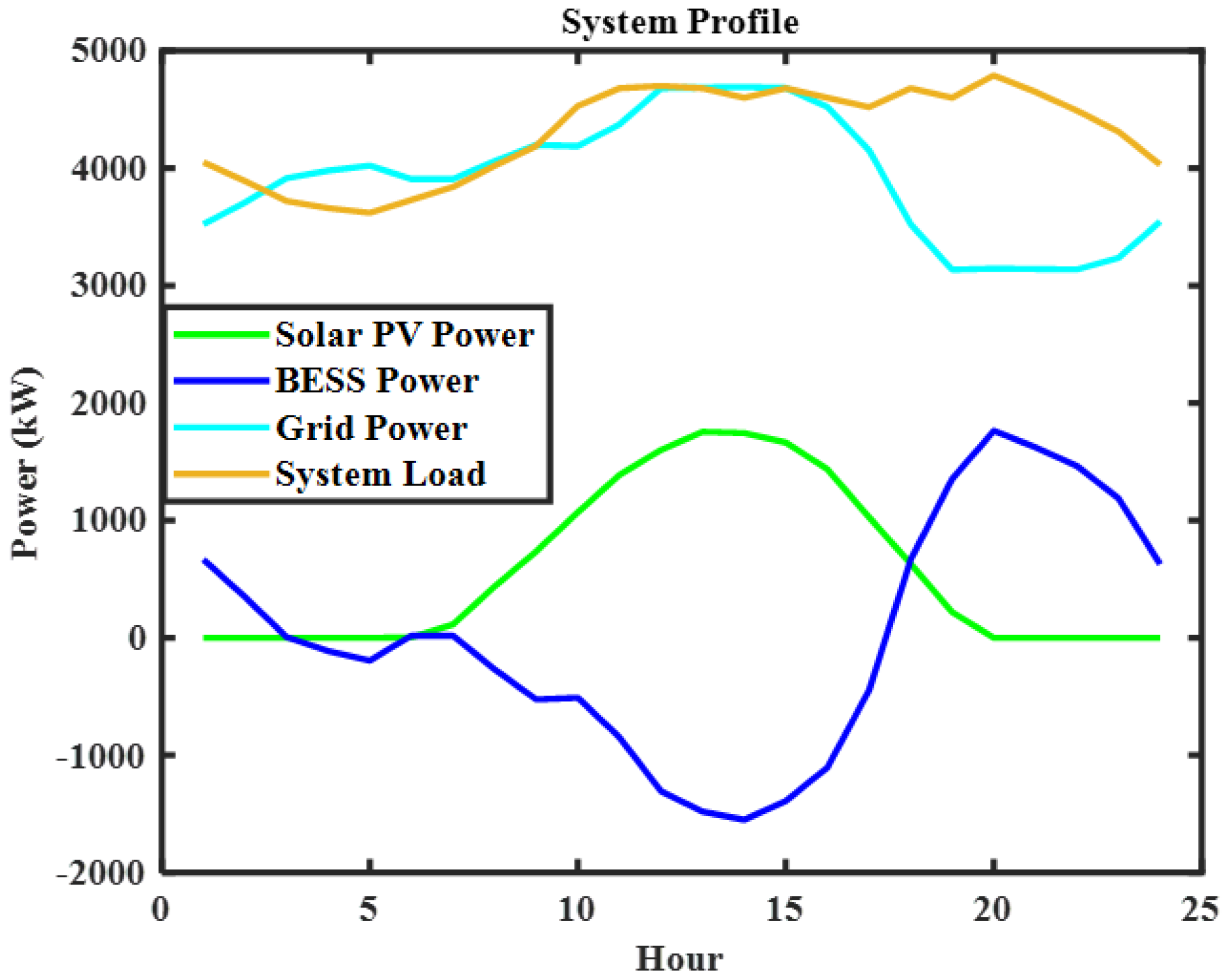
A.2. Comparison of System Parameters for Deterministic and Polynomial Multiple Regression (PMR) Approaches for Modified Real 94-Bus Portuguese RDS (MRBPRDS)
| Parameters | Deterministic Approach (BESS Size = 1.8 MW) | PMR Approach (BESS Size = 1.84 MW) |
|---|---|---|
| PSI |  |  |
| VSI | 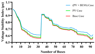 | 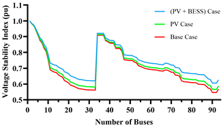 |
| Bus voltage profile | 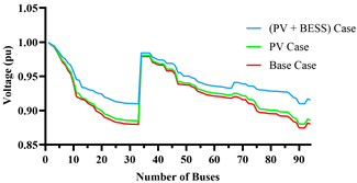 | 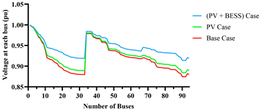 |
| System profile | 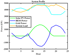 | 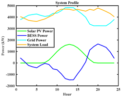 |
References
- Alzahrani, A.; Alharthi, H.; Khalid, M. Minimization of Power Losses through Optimal Battery Placement in a Distributed Network with High Penetration of Photovoltaics. Energies 2020, 13, 140. [Google Scholar] [CrossRef]
- Alshahrani, A.; Omer, S.; Su, Y.; Mohamed, E.; Alotaibi, S. The Technical Challenges Facing the Integration of Small-Scale and Large-scale PV Systems into the Grid: A Critical Review. Electronics 2019, 8, 1443. [Google Scholar] [CrossRef]
- Hameed, Z.; Hashemi, S.; Træholt, C. Site Selection Criteria for Battery Energy Storage in Power Systems. In Proceedings of the 2020 IEEE Canadian Conference on Electrical and Computer Engineering (CCECE), London, ON, Canada, 30 August–2 September 2020; pp. 1–7. [Google Scholar]
- Mohamad, F.; Teh, J.; Lai, C.-M.; Chen, L.-R. Development of Energy Storage Systems for Power Network Reliability: A Review. Energies 2018, 11, 2278. [Google Scholar] [CrossRef]
- Abdolahi, A.; Salehi, J.; Samadi Gazijahani, F.; Safari, A. Probabilistic multi-objective arbitrage of dispersed energy storage systems for optimal congestion management of active distribution networks including solar/wind/CHP hybrid energy system. J. Renew. Sustain. Energy 2018, 10, 045502. [Google Scholar] [CrossRef]
- Zhengmao, L.; Yan, X.; Sidun, F.; Yu, W. Multi-objective Coordinated Energy Dispatch and Voyage Scheduling for a Multi-energy Cruising Ship. In Proceedings of the 2019 IEEE/IAS 55th Industrial and Commercial Power Systems Technical Conference (I&CPS), Calgary, AB, Canada, 5–8 May 2019; pp. 1–8. [Google Scholar]
- Matthiss, B.; Momenifarahani, A.; Binder, J. Storage Placement and Sizing in a Distribution Grid with High PV Generation. Energies 2021, 14, 303. [Google Scholar] [CrossRef]
- Nor, N.M.; Ali, A.; Ibrahim, T.; Romlie, M.F. Battery Storage for the Utility-Scale Distributed Photovoltaic Generations. IEEE Access 2018, 6, 1137–1154. [Google Scholar] [CrossRef]
- Szultka, A.; Szultka, S.; Czapp, S.; Lubosny, Z.; Malkowski, R. Integrated Algorithm for Selecting the Location and Control of Energy Storage Units to Improve the Voltage Level in Distribution Grids. Energies 2020, 13, 6720. [Google Scholar] [CrossRef]
- Yuan, Z.; Wang, W.; Wang, H.; Yildizbasi, A. A new methodology for optimal location and sizing of battery energy storage system in distribution networks for loss reduction. J. Energy Storage 2020, 29, 101368. [Google Scholar] [CrossRef]
- Mohamed, A.A.R.; Morrow, D.J.; Best, R.J.; Bailie, I.; Cupples, A.; Pollock, J. Battery Energy Storage Systems Allocation Considering Distribution Network Congestion. In Proceedings of the 2020 IEEE PES Innovative Smart Grid Technologies Europe (ISGT-Europe), Hague, The Netherlands, 26–28 October 2020; pp. 1015–1019. [Google Scholar]
- Meena, N.K.; Parashar, S.; Swarnkar, A.; Gupta, N.; Niazi, K.R. Improved Elephant Herding Optimization for Multiobjective DER Accommodation in Distribution Systems. IEEE Trans. Ind. Inform. 2018, 14, 1029–1039. [Google Scholar] [CrossRef]
- Zhang, Y.; Ren, S.; Dong, Z.Y.; Xu, Y.; Meng, K.; Zheng, Y. Optimal placement of battery energy storage in distribution networks considering conservation voltage reduction and stochastic load composition. IET Gener. Transm. Dis. 2017, 11, 3862–3870. [Google Scholar] [CrossRef]
- Shafiq, S.; Khan, B.; Al-Awami, A.T. Optimal Battery Placement in Distribution Network Using Voltage Sensitivity Approach. In Proceedings of the 2019 IEEE Power and Energy Conference at Illinois (PECI), Champaign, IL, USA, 28 February–1 March 2019; p. 8698781. [Google Scholar]
- Khunkitti, S.; Boonluk, P.; Siritaratiwat, A. Optimal Location and Sizing of BESS for Performance Improvement of Distribution Systems with High DG Penetration. Int. Trans. Electr. Energy Syst. 2022, 2022, 6361243. [Google Scholar] [CrossRef]
- Damian, S.; Wong, L.A. Optimal Energy Storage Placement and Sizing in Distribution System. In Proceedings of the 2022 IEEE International Conference in Power Engineering Application (ICPEA), Shah Alam, Malaysia, 7–8 March 2022; pp. 1–6. [Google Scholar]
- Li, X.; Hu, C.; Luo, S.; Lu, H.; Piao, Z.; Jing, L. Distributed Hybrid-Triggered Observer-Based Secondary Control of Multi-Bus DC Microgrids Over Directed Networks. IEEE Trans. Circuits Syst. I Regul. Pap. 2025, 1–14. [Google Scholar] [CrossRef]
- López, L.; López, I.; Gomez-Cornejo, J.; Aranzabal, I.; Eguia, P. Analysis of impact for PV-BES strategies in low-voltage distribution system. Electr. Eng. 2024, 107, 2147–2162. [Google Scholar] [CrossRef]
- Till, J.; You, S.; Liu, Y.; Du, P. Impact of High PV Penetration on Voltage Stability. In Proceedings of the 2020 IEEE/PES Transmission and Distribution Conference and Exposition (T&D), Chicago, IL, USA, 12–15 October 2020. [Google Scholar]
- Abdel-Mawgoud, H.; Kamel, S.; Tostado-Véliz, M.; Elattar, E.E.; Hussein, M.M. Optimal Incorporation of Photovoltaic Energy and Battery Energy Storage Systems in Distribution Networks Considering Uncertainties of Demand and Generation. Appl. Sci. 2021, 11, 8231. [Google Scholar] [CrossRef]
- Khasanov, M.; Kamel, S.; Hassan, M.H.; Domínguez-García, J.L. Maximizing renewable energy integration with battery storage in distribution systems using a modified Bald Eagle Search Optimization Algorithm. Neural Comput. Appl. 2024, 36, 8577–8605. [Google Scholar] [CrossRef]
- NASA. NASA Prediction Of Worldwide Energy Resources (POWER). Available online: https://power.larc.nasa.gov/data-access-viewer/ (accessed on 29 March 2025).
- Dehnavi, E.; Afsharnia, S.; Gholami, K. Optimal allocation of unified power quality conditioner in the smart distribution grids. Electr. Eng. 2019, 101, 1277–1293. [Google Scholar] [CrossRef]
- Hi-MO 5m (G2). LR5-72HPH 540~560M; LONGi: Shanghai, China, 2022. [Google Scholar]
- Maleki, A.; Askarzadeh, A. Comparative study of artificial intelligence techniques for sizing of a hydrogen-based stand-alone photovoltaic/wind hybrid system. Int. J. Hydrogen Energy 2014, 39, 9973–9984. [Google Scholar] [CrossRef]
- Aman, M.M.; Jasmon, G.B.; Mokhlis, H.; Bakar, A.H.A. Optimal placement and sizing of a DG based on a new power stability index and line losses. Int. J. Electr. Power Energy Syst. 2012, 43, 1296–1304. [Google Scholar] [CrossRef]
- Danish, M.S.S.; Senjyu, T.; Danish, S.M.S.; Sabory, N.R.; K, N.; Mandal, P. A Recap of Voltage Stability Indices in the Past Three Decades. Energies 2019, 12, 1544. [Google Scholar] [CrossRef]
- Kolios, A.; Mytilinou, V.; Lozano-Minguez, E.; Salonitis, K. A Comparative Study of Multiple-Criteria Decision-Making Methods under Stochastic Inputs. Energies 2016, 9, 566. [Google Scholar] [CrossRef]
- Qiu, Y.; Yang, X.; Chen, S. An improved gray wolf optimization algorithm solving to functional optimization and engineering design problems. Sci. Rep. 2024, 14, 14190. [Google Scholar] [CrossRef] [PubMed]
- Altayara, I.A.; Al-Ammar, E.A.; Ghazi, G.A.; Katheri, A.A.A. Optimal Allocation of Distributed Generation Using Modified Grey Wolf Optimizer. In Proceedings of the 2022 International Conference on Automation, Computing and Renewable Systems (ICACRS), Pudukkottai, India, 13–15 December 2022; pp. 884–889. [Google Scholar]
- Gandhi, K.J.; Patil, N. Solving Economic Load Dispatch Problem using Grey Wolf Optimizer Method. Int. J. Recent Technol. Eng. 2019, 8, 684–688. [Google Scholar] [CrossRef]
- Nimma, K.S.; Al-Falahi, M.D.A.; Nguyen, H.D.; Jayasinghe, S.D.G.; Mahmoud, T.S.; Negnevitsky, M. Grey Wolf Optimization-Based Optimum Energy-Management and Battery-Sizing Method for Grid-Connected Microgrids. Energies 2018, 11, 847. [Google Scholar] [CrossRef]
- Miao, D.; Hossain, S. Improved gray wolf optimization algorithm for solving placement and sizing of electrical energy storage system in micro-grids. ISA Trans. 2020, 102, 376–387. [Google Scholar] [CrossRef] [PubMed]
- Mirjalili, S.; Mirjalili, S.M.; Lewis, A. Grey Wolf Optimizer. Adv. Eng. Softw. 2014, 69, 46–61. [Google Scholar] [CrossRef]
- Hou, Y.; Gao, H.; Wang, Z.; Du, C. Improved Grey Wolf Optimization Algorithm and Application. Sensors 2022, 22, 3810. [Google Scholar] [CrossRef]
- Hwang, C.-L.; Yoon, K. Methods for Multiple Attribute Decision Making. In Multiple Attribute Decision Making: Methods and Applications A State-of-the-Art Survey; Springer: Berlin/Heidelberg, Germany, 1981; pp. 58–191. [Google Scholar]
- Galgali, V.S.; Ramachandran, M.; Vaidya, G.A. Multi-Objective Optimal Placement and Sizing of DGs by Hybrid Fuzzy TOPSIS and Taguchi Desirability Function Analysis Approach. Electr. Power Compon. Syst. 2021, 48, 2144–2155. [Google Scholar] [CrossRef]
- Elkadeem, M.R.; Elaziz, M.A.; Ullah, Z.; Wang, S.; Sharshir, S.W. Optimal Planning of Renewable Energy-Integrated Distribution System Considering Uncertainties. IEEE Access 2019, 7, 164887–164907. [Google Scholar] [CrossRef]
- Malik, M.Z.; Kumar, M.; Soomro, A.M.; Baloch, M.H.; Farhan, M.; Gul, M.; Kaloi, G.S. Strategic planning of renewable distributed generation in radial distribution system using advanced MOPSO method. Energy Rep. 2020, 6, 2872–2886. [Google Scholar] [CrossRef]


| Sr. No. | Parameter (Symbol) | Value | Unit |
|---|---|---|---|
| 1 | Rated power of solar PV panel (PRS) | 550 | Wp |
| 2 | Ambient temperature (TA) | 19.19 | °C |
| 3 | Cell temperature (TC) | 25 | °C |
| 4 | Normal Operating Cell Temperature (TNOCT) | 45 | °C |
| 5 | Short-Circuit Current (ISC) | 11.29 | A |
| 6 | Current at Maximum Power Point (IMPP) | 10.51 | A |
| 7 | Current temperature coefficient (Ki) | 0.05 | A/°C |
| 8 | Open-Circuit Voltage (Voc) | 46.82 | V |
| 9 | Voltage at Maximum Power Point (VMPP) | 39.14 | V |
| 10 | Voltage temperature coefficient (Kv) | −0.265 | V/°C |
| 11 | Efficiency of PV panel | 21.3 | % |
| 12 | Length of PV panel | 2.278 | M |
| 13 | Width of PV panel | 1.134 | M |
| Case Number | Deterministic Approach | Probabilistic Beta PDF Approach | Polynomial Multiple Regression Approach | |||||||||
|---|---|---|---|---|---|---|---|---|---|---|---|---|
| Simultaneous OPSBESS | Sequential OPSBESS | Simultaneous OPSBESS | Sequential OPSBESS | Simultaneous OPSBESS | Sequential OPSBESS | |||||||
| BESS Location (Size, MW) | System Losses (MWh) | BESS Location (Size, MW) | System Losses (MWh) | BESS Location (Size, MW) | System Losses (MWh) | BESS Location (Size, MW) | System Losses (MWh) | BESS Location (Size MW) | System Losses (MWh) | BESS Location (Size, MW) | System Losses (MWh) | |
| Case I | No PV and No BESS (W1 = 1, W2 = W3 = 0) | |||||||||||
| IGT | - | 2.649 | - | 2.649 | - | 2.649 | - | 2.649 | - | 2.649 | - | 2.649 |
| IPT | - | 2.649 | - | 2.649 | - | 2.649 | - | 2.649 | - | 2.649 | - | 2.649 |
| Case II | With 3 PV Systems and No BESS (W1 = 1, W2 = W3 = 0) | |||||||||||
| IGT | No BESS | 2.170 | No BESS | 2.170 | No BESS | 2.064 | No BESS | 2.064 | No BESS | 2.162 | No BESS | 2.162 |
| IPT | No BESS | 2.170 | No BESS | 2.170 | No BESS | 2.064 | No BESS | 2.064 | No BESS | 2.162 | No BESS | 2.162 |
| Case III A | With 3 PV Systems and 1 BESS Unit (Aggregated BESS) (W1 = 1, W2 = W3 = 0) | |||||||||||
| IGT | 30(2.326) | 2.212 | 30(2.326) | 2.212 | 29(2.414) | 2.017 | 29(2.414) | 2.017 | 30(2.324) | 2.186 | 30 (2.324) | 2.186 |
| IPT | 30(2.270) | 2.168 | 30(2.270) | 2.168 | 29(2.356) | 1.980 | 29(2.356) | 1.980 | 30(2.266) | 2.140 | 30 (2.266) | 2.140 |
| Case III B | With 3 PV Systems and 1 BESS Unit (Aggregated BESS) (W1 = 0.4, W2 = W3 = 0.3) | |||||||||||
| IGT | 26 (2.30) | 1.890 | 26 (2.30) | 1.890 | 26 (2.42) | 1.785 | 26 (2.42) | 1.785 | 26 (2.40) | 1.871 | 26 (2.40) | 1.871 |
| IPT | 26 (2.26) | 1.899 | 26 (2.26) | 1.899 | 26 (2.36) | 1.867 | 26 (2.36) | 1.867 | 26 (2.27) | 1.882 | 26 (2.27) | 1.882 |
| Case IV | With 3 PV Systems and 2 BESS Units (W1 = 0.4, W2 = W3 = 0.3) | |||||||||||
| IGT | 14 (1.60) | 1.832 | 26 (1.89) | 1.810 | 7 (0.65) | 1.769 | 26 (2.09) | 1.735 | 7 (0.98) | 1.835 | 26 (1.99) | 1.812 |
| 30 (0.70) | 18 (0.43) | 26 (1.77) | 18 (0.33) | 25 (1.51) | 18 (0.45) | |||||||
| IPT | 14 (0.55) | 1.867 | 26 (1.98) | 1.860 | 15 (0.55) | 1.850 | 26 (1.80) | 1.845 | 14 (0.49) | 1.860 | 26 (1.98) | 1.855 |
| 27 (1.71) | 18 (0.28) | 27 (1.81) | 30 (0.56) | 19 (1.77) | 18 (0.29) | |||||||
| Case V | With 3 PV Systems and 3 BESS Units (W1 = 0.4, W2 = W3 = 0.3) | |||||||||||
| IGT | 18 (0.58) | 1.737 | 26 (1.67) | 1.719 | 12 (0.64) | 1.724 | 26 (1.51) | 1.631 | 7 (0.67) | 1.741 | 26 (1.60) | |
| 26 (1.16) | 18 (0.44) | 26 (1.36) | 18 (0.63) | 26 (1.24) | 18 (0.50) | 1.702 | ||||||
| 30 (0.57) | 25 (0.21) | 32 (0.41) | 30 (0.26) | 30 (0.51) | 32 (0.21) | |||||||
| IPT | 15 (0.47) | 1.755 | 26 (1.54) | 1.741 | 15 (0.39) | 1.735 | 26 (1.75) | 1.685 | 25 (0.43) | 1.750 | 26 (1.66) | 1.739 |
| 26 (0.94) | 18 (0.49) | 19 (0.83) | 18 (0.33) | 26 (1.09) | 18 (0.39) | |||||||
| 30 (0.85) | 25 (0.23) | 26 (1.13) | 30 (0.28) | 30 (0.74) | 30 (0.22) | |||||||
| Case Number | Deterministic Approach | Probabilistic Beta PDF Approach | Polynomial Multiple Regression Approach | |||||||||
|---|---|---|---|---|---|---|---|---|---|---|---|---|
| Simultaneous OPSBESS | Sequential OPSBESS | Simultaneous OPSBESS | Sequential OPSBESS | Simultaneous OPSBESS | Sequential OPSBESS | |||||||
| BESS Location (Size, MW) | System Losses (MWh) | BESS Location (Size, MW) | System Losses (MWh) | BESS Location (Size, MW) | System Losses (MWh) | BESS Location (Size, MW) | System Losses (MWh) | BESS Location (Size MW) | System Losses (MWh) | BESS Location (Size, MW) | System Losses (MWh) | |
| Case I | No PV and No BESS (W1 = 1, W2 = W3 = 0) | |||||||||||
| IGT | - | 6.772 | - | 6.772 | - | 6.772 | - | 6.772 | - | 6.772 | - | 6.772 |
| IPT | - | 6.772 | - | 6.772 | - | 6.772 | - | 6.772 | - | 6.772 | - | 6.772 |
| Case II | With 3 PV Systems and No BESS (W1 = 1, W2 = W3 = 0) | |||||||||||
| IGT | No BESS | 5.382 | No BESS | 5.382 | No BESS | 5.108 | No BESS | 5.108 | No BESS | 5.378 | No BESS | 5.378 |
| IPT | No BESS | 5.382 | No BESS | 5.382 | No BESS | 5.108 | No BESS | 5.108 | No BESS | 5.378 | No BESS | 5.378 |
| Case III A | With 3 PV Systems and 1 BESS Unit (Aggregated BESS) (W1 = 1, W2 = W3 = 0) | |||||||||||
| IGT | 19 (1.8) | 4.837 | 19 (1.8) | 4.838 | 19 (1.96) | 4.552 | 19 (1.96) | 4.552 | 19 (1.84) | 4.846 | 19 (1.84) | 4.846 |
| IPT | 19 (1.8) | 4.838 | 19 (1.8) | 4.838 | 19 (1.96) | 4.553 | 19 (1.96) | 4.553 | 19 (1.84) | 4.847 | 19 (1.84) | 4.847 |
| Case III B | With 3 PV Systems and 1 BESS Unit (Aggregated BESS) (W1 = 0.4, W2 = W3 = 0.3) | |||||||||||
| IGT | 20 (1.8) | 4.902 | 20 (1.8) | 4.902 | 20 (1.96) | 4.580 | 20 (1.96) | 4.617 | 20 (1.84) | 4.869 | 20 (1.84) | 4.869 |
| IPT | 20 (1.8) | 4.902 | 20 (1.8) | 4.902 | 20 (1.96) | 4.580 | 20 (1.96) | 4.553 | 20 (1.84) | 4.870 | 20 (1.84) | 4.870 |
| Case IV | With 3 PV Systems and 2 BESS Units (W1 = 0.4, W2 = W3 = 0.3) | |||||||||||
| IGT | 77 (1.09) | 4.639 | 20 (1.00) | 4.620 | 77 (1.21) | 4.356 | 20 (1.37) | 4.325 | 77 (1.38) | 4.681 | 20 (1.67) | 4.621 |
| 61 (0.75) | 58 (0.8) | 88 (0.74) | 58 (0.58) | 61 (0.45) | 58 (0.17) | |||||||
| IPT | 58 (1.44) | 4.640 | 20 (1.09) | 4.639 | 58 (1.17) | 4.356 | 20 (1.25) | 4.339 | 77 (1.38) | 4.703 | 20 (1.37) | 4.693 |
| 77 (0.40) | 58 (0.75) | 77 (0.79) | 58 (0.71) | 61 (0.47) | 58 (0.48) | |||||||
| Case V | With 3 PV Systems and 3 BESS Units (W1 = 0.4, W2 = W3 = 0.3) | |||||||||||
| IGT | 20 (1.02) | 4.613 | 20 (0.87) | 4.616 | 58 (0.68) | 4.391 | 20 (1.26) | 4.335 | 20 (0.92) | 4.632 | 20 (1.56) | 4.612 |
| 58 (0.1) | 58 (0.72) | 77 (0.75) | 58 (0.54) | 58 (0.52) | 58 (0.20) | |||||||
| 77 (0.72) | 84 (0.23) | 84 (0.52) | 84 (0.15) | 77 (0.40) | 84 (0.07) | |||||||
| IPT | 20 (0.45) | 4.631 | 20 (1.058) | 4.615 | 58 (1.22) | 4.365 | 20 (1.35) | 4.352 | 20 (0.87) | 4.704 | 20 (1.35) | 4.703 |
| 27 (0.78) | 50 (0.04) | 77 (0.72) | 58 (0.53) | 59 (0.58) | 58 (0.42) | |||||||
| 59 (0.61) | 58 (0.75) | 84 (0.02) | 92 (0.08) | 84 (0.40) | 92 (0.08) | |||||||
| Sr. No. | Paper | Resource Uncertainty | MOF | Optimization Techniques | APL (kW) | PSI (pu) | VSI (pu) | DG/BESS Size (MW) and Location |
|---|---|---|---|---|---|---|---|---|
| IEEE 33-bus RDS | ||||||||
| 1 | Arya Abdolahi [5] | PV by Beta PDF; wind by Weibull PDF | Congestion alleviation and procurement cost minimization | MOPSO | Not mentioned | - | - | 2 PVs @ Bus 11, 22; 2 WTs @ Bus 6, 32; 2 CHP @ Bus 16, 26; 6 BESSs @ Bus 5, 10, 14, 20, 24,31. Total DG Size = not mentioned. |
| 2 | Mohd Nor [7] | PV by Beta PDF | ELI and VD | GA | 14,773.75 | - | - | PV of 3.3 @ Bus 6; BESS of 1.84 @ Bus 6. Total DG Size = 3.3 MW. |
| 3 | Elkadeem [36] | PV by Beta PDF | Loss, VSI, VD, and AEL | HHO | 83.0964 | - | (28.828) or 0.9 * | 3 PVs (0.761 @ Bus 14; 1.0947 @ Bus 24; 1.0684 @ Bus 30); 3 WTs (0.8204 @ Bus 14; 1.173 @ Bus 24; 1.481 @ Bus 30). Total DG Size = 6.3985 MW. |
| 4 | Proposed Work | PV by Beta PDF and PMR | APL, PSI, and VSI (W1 = 0.4, W2 = W3 = 0.3) | IGWO | 74.375 | 0.01 | 0.8 | PV of 0.6 MW @ Bus 18, 25, 30; BESS of 2.42 @ Bus 26. Total DG Size = 1.8 MW. |
| Real 94-bus Portuguese RDS | ||||||||
| 5 | Elkadeem [36] | PV by Beta PDF | Loss, VSI, VD, and AEL | HHO | 213.661 | - | (76.384) or 0.82 * | 1 PV (2.636 @ Bus 19); 1 WT (2.968 @ Bus 19). Total DG Size = 5.604 MW. |
| 6 | Proposed Work | PV by Beta PDF and PMR | APL, PSI, and VSI (W1 = 0.4, W2 = W3 = 0.3) | IGWO | 192.375 | 0.01 | 0.62 | PV of 0.8 MW @ Bus 19, 58, 84; BESS of 1.96 @ Bus 20. Total DG Size = 2.4 MW. |
Disclaimer/Publisher’s Note: The statements, opinions and data contained in all publications are solely those of the individual author(s) and contributor(s) and not of MDPI and/or the editor(s). MDPI and/or the editor(s) disclaim responsibility for any injury to people or property resulting from any ideas, methods, instructions or products referred to in the content. |
© 2025 by the authors. Licensee MDPI, Basel, Switzerland. This article is an open access article distributed under the terms and conditions of the Creative Commons Attribution (CC BY) license (https://creativecommons.org/licenses/by/4.0/).
Share and Cite
Karve, G.M.; Thakare, M.S.; Vaidya, G.A. Optimal Siting and Sizing of Battery Energy Storage System in Distribution System in View of Resource Uncertainty. Energies 2025, 18, 2340. https://doi.org/10.3390/en18092340
Karve GM, Thakare MS, Vaidya GA. Optimal Siting and Sizing of Battery Energy Storage System in Distribution System in View of Resource Uncertainty. Energies. 2025; 18(9):2340. https://doi.org/10.3390/en18092340
Chicago/Turabian StyleKarve, Gauri Mandar, Mangesh S. Thakare, and Geetanjali A. Vaidya. 2025. "Optimal Siting and Sizing of Battery Energy Storage System in Distribution System in View of Resource Uncertainty" Energies 18, no. 9: 2340. https://doi.org/10.3390/en18092340
APA StyleKarve, G. M., Thakare, M. S., & Vaidya, G. A. (2025). Optimal Siting and Sizing of Battery Energy Storage System in Distribution System in View of Resource Uncertainty. Energies, 18(9), 2340. https://doi.org/10.3390/en18092340