
Modeling Ecological Risk in Bottom Sediments Using Predictive Data Analytics: Implications for Energy Systems

 , ,
, ,  , , and
Abstract
1. Introduction
1.1. Literature Review
1.2. Problem Statement
1.3. Objective
2. Materials and Methods
2.1. Study Area and Data for Statistical Analyses
2.2. Multiple Linear Regression Models
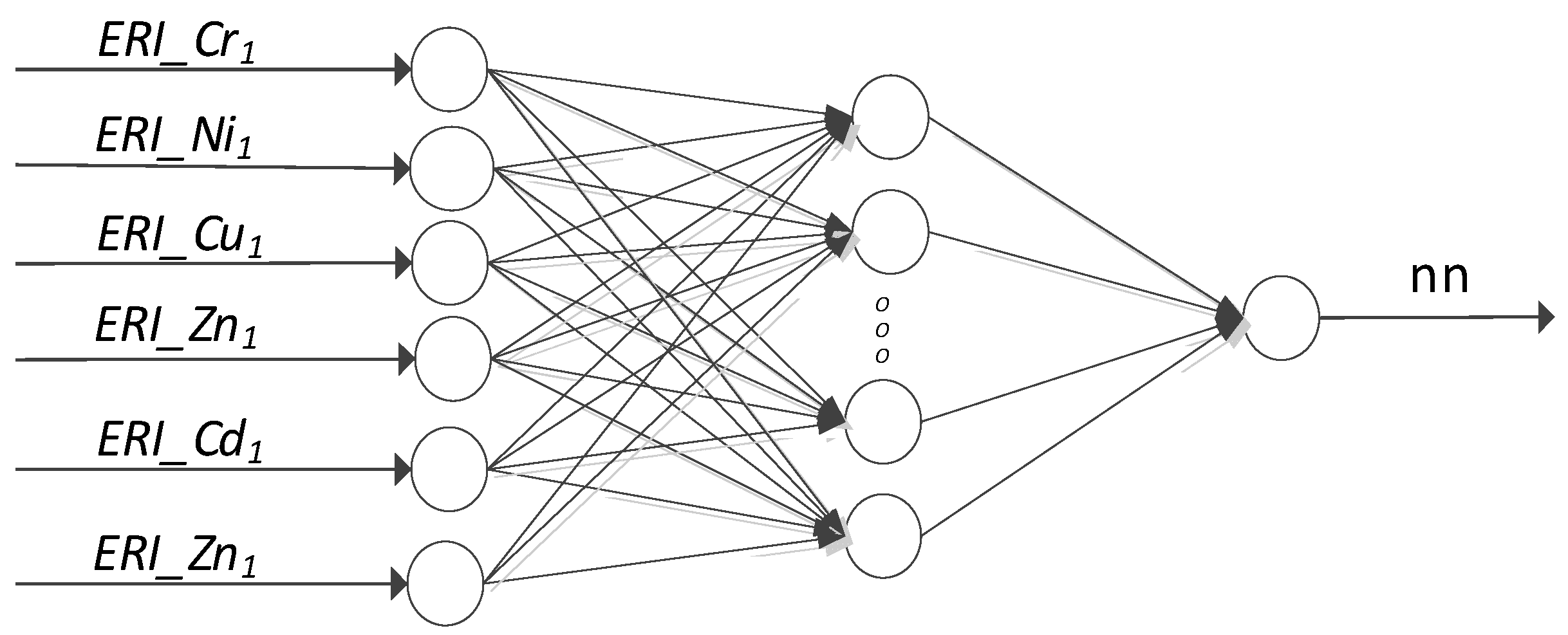
2.3. Artificial Neural Network Models
2.4. Model Quality Indicators
2.5. Statistical Analysis of Prediction Results
3. Results
3.1. Multiple Linear Regression Models
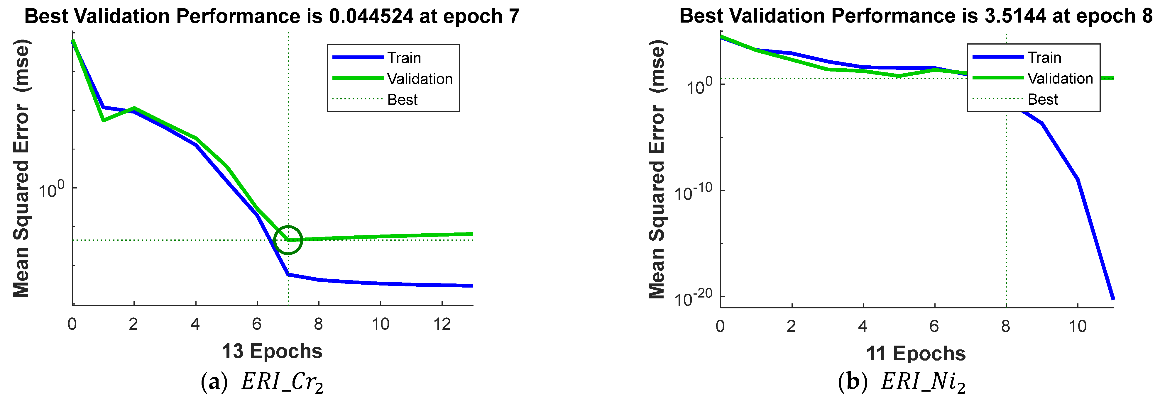
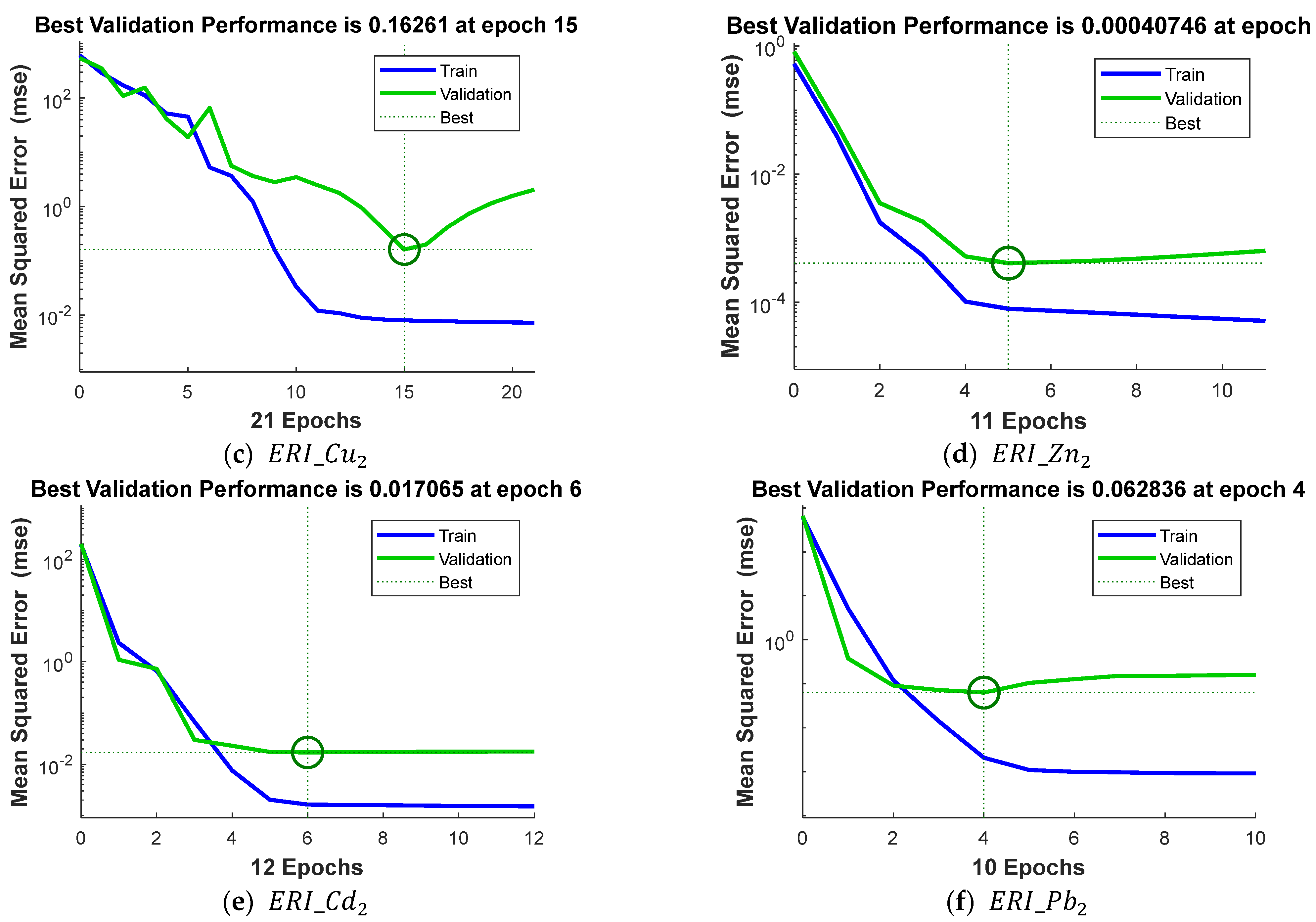
3.2. Artificial Neural Network
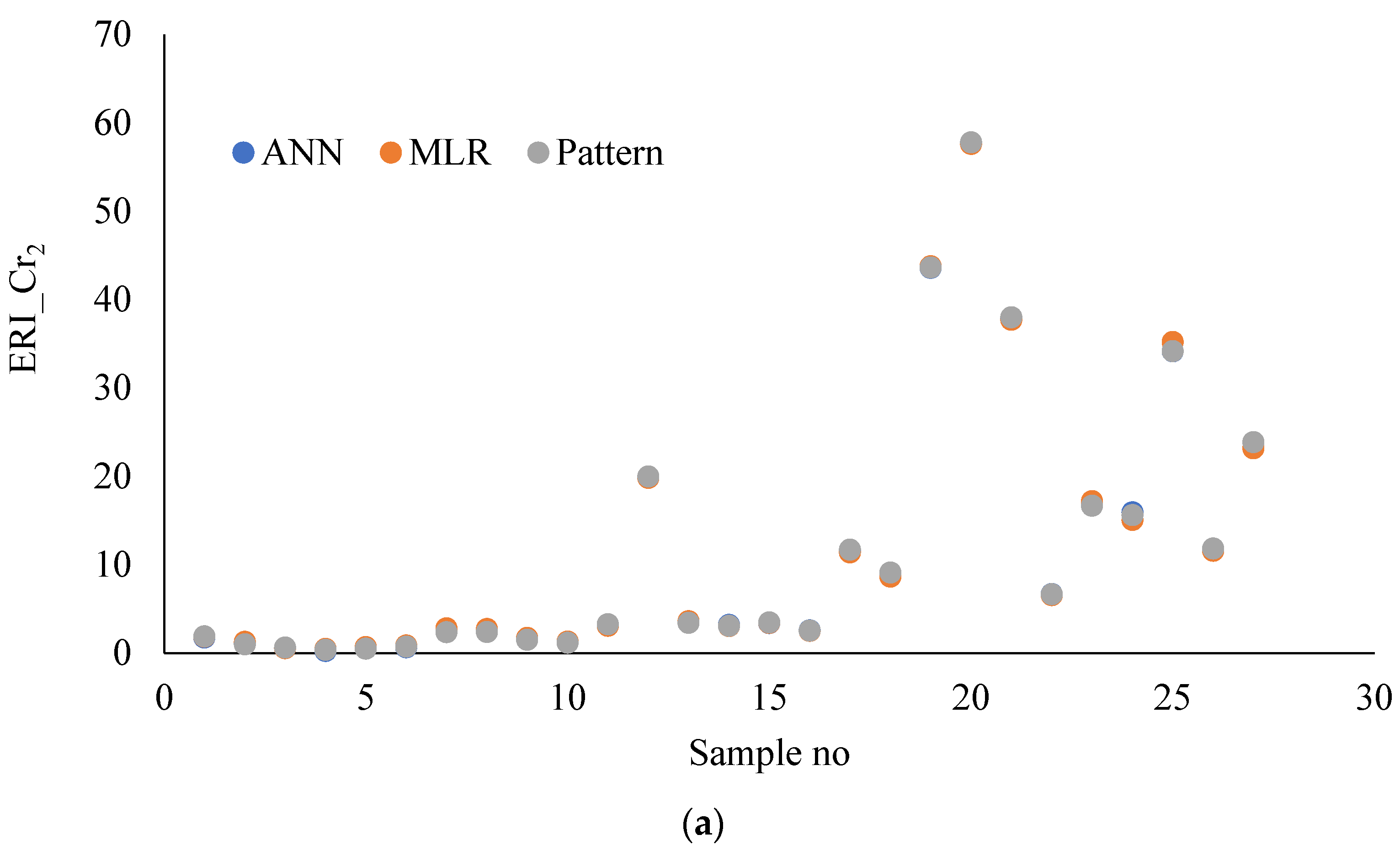
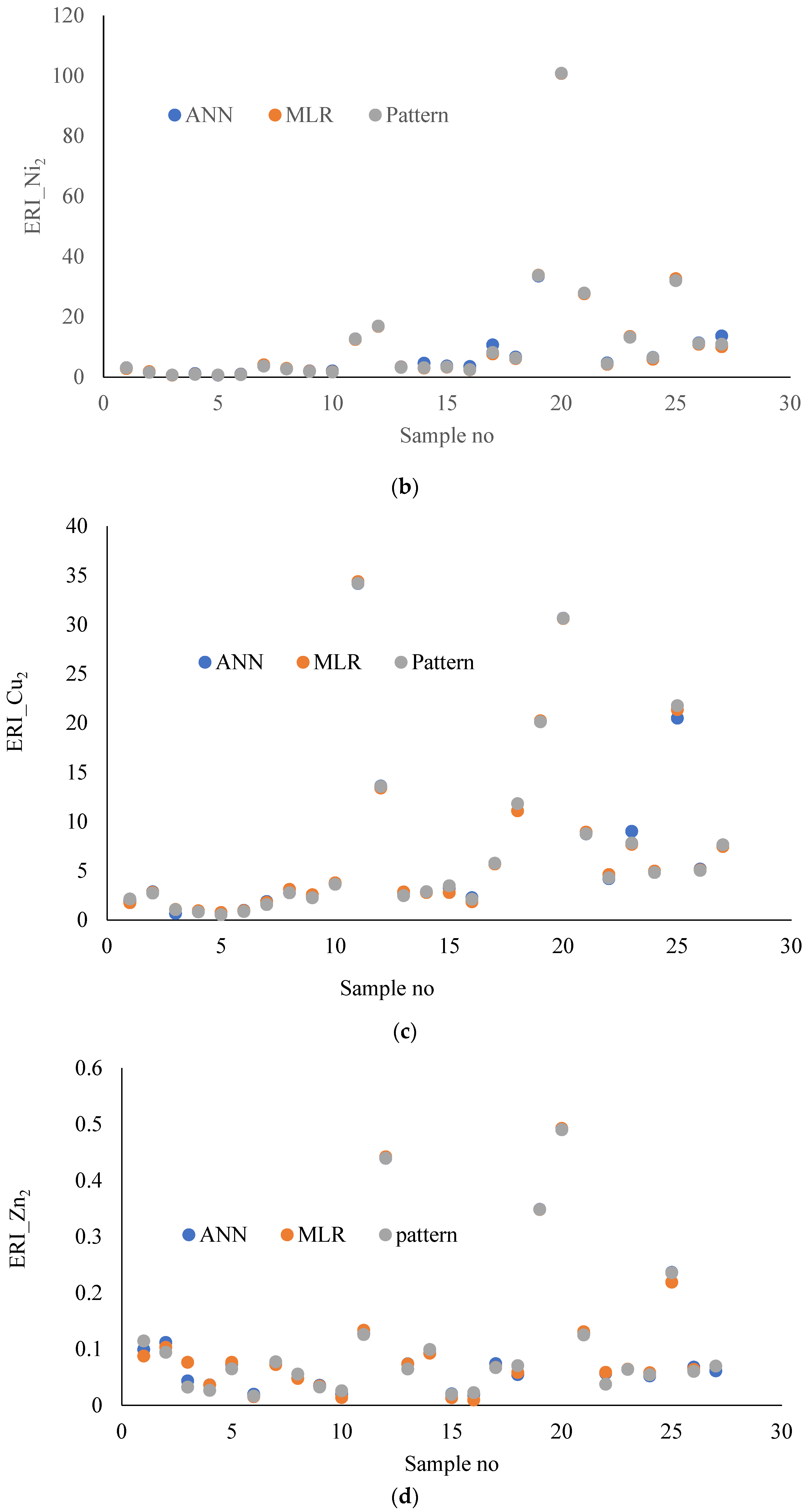
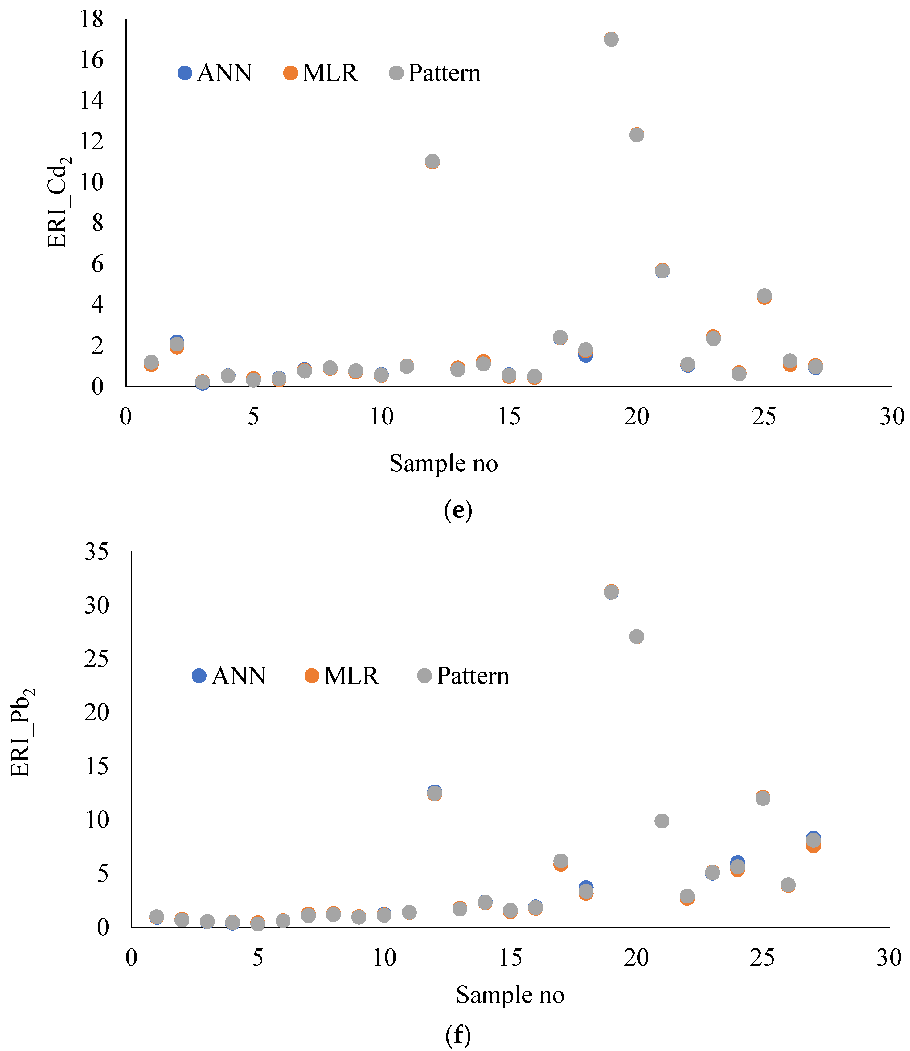
3.3. Comparison of MLR and ANN Models
4. Conclusions
Author Contributions
Funding
Data Availability Statement
Conflicts of Interest
References
- Li, S.; Xu, Y.J.; Ni, M. Changes in Sediment, Nutrients and Major Ions in the World Largest Reservoir: Effects of Damming and Reservoir Operation. J. Clean. Prod. 2021, 318, 128601. [Google Scholar] [CrossRef]
- Akhtar, N.; Syakir Ishak, M.I.; Bhawani, S.A.; Umar, K. Various natural and anthropogenic factors responsible for water quality degradation: A review. Water 2021, 13, 2660. [Google Scholar] [CrossRef]
- Chen, X.; Wang, Y.; Sun, T.; Huang, Y.; Chen, Y.; Zhang, M.; Ye, C. Effects of Sediment Dredging on Nutrient Release and Eutrophication in the Gate-Controlled Estuary of Northern Taihu Lake. J. Chem. 2021, 2021, 1–13. [Google Scholar] [CrossRef]
- Dalu, T.; Tshivhase, R.; Cuthbert, R.N.; Murungweni, F.M.; Wasserman, R.J. Metal Distribution and Sediment Quality Variation Declared Wetland. Water 2020, 12, 2779. [Google Scholar] [CrossRef]
- Xu, Q.; Zhou, K.; Wu, B. Dam Construction Reshapes Heavy Metal Pollution in Soil/Sediment in the Three Gorges Reservoir, China, from 2008 to 2020. Front. Environ. Sci. 2023, 11, 1269138. [Google Scholar] [CrossRef]
- Sojka, M.; Jaskuła, J.; Barabach, J.; Ptak, M.; Zhu, S. Heavy metals in lake surface sediments in protected areas in Poland: Concentration, pollution, ecological risk, sources and spatial distribution. Sci. Rep. 2022, 12, 15006. [Google Scholar] [CrossRef]
- Hossain, M.A.; Furumai, H.; Nakajima, F.; Aryal, R.K. Heavy metals speciation in sediment accumulated within an infiltration facility and evaluation of metal retention properties of underlying soil. Water Sci. Technol. 2007, 56, 827–834. [Google Scholar] [CrossRef]
- Shahbazi, K.; Beheshti, M. Comparison of three methods for measuring heavy metals in calcareous soils of Iran. SN Appl. Sci. 2019, 1, 1541. [Google Scholar] [CrossRef]
- Sastre, J.; Sahuquillo, A.; Vidal, M.; Rauret, G. Determination of Cd, Cu, Pb and Zn in environmental samples: Microwave-assisted total digestion versus aqua regia and nitric acid extraction. Anal. Chim. Acta 2002, 462, 59–72. [Google Scholar] [CrossRef]
- Zhong, X.L.; Zhou, S.L.; Zhu, Q.; Zhao, Q.G. Fraction distribution and bioavailability of soil heavy metals in the Yangtze River Delta-A case study of Kunshan City in Jiangsu Province, China. J. Hazard. Mater. 2011, 198, 13–21. [Google Scholar] [CrossRef]
- Brady, J.P.; Ayoko, G.A.; Martens, W.N.; Goonetilleke, A. Development of a hybrid pollution index for heavy metals in marine and estuarine sediments. Environ. Monit. Assess. 2015, 187, 306. [Google Scholar] [CrossRef]
- Bhagat, S.K.; Tung, T.M.; Yaseen, Z.M. Heavy metal contamination prediction using ensemble model: Case study of Bay sedimentation, Australia. J. Hazard. Mater. 2021, 403, 123492. [Google Scholar] [CrossRef] [PubMed]
- Aljahdali, M.O.; Alhassan, A.B. Ecological risk assessment of heavy metal contamination in mangrove habitats, using biochemical markers and pollution indices: A case study of Avicennia marina L. in the Rabigh lagoon, Red Sea. Saudi J. Biol. Sci. 2020, 27, 1174–1184. [Google Scholar] [CrossRef] [PubMed]
- Sidoruk, M. Pollution and Potential Ecological Risk Evaluation of Heavy Metals in the Bottom Sediments: A Case Study of Eutrophic Bukwałd Lake Located in an Agricultural Catchment. Int. J. Environ. Res. Public Health 2023, 20, 2387. [Google Scholar] [CrossRef] [PubMed]
- Ramseyer, C.A.; Miller, P.W.; Mote, T.L. Future precipitation variability during the early rainfall season in the El Yunque National Forest. Sci. Total Environ. 2019, 661, 326–336. [Google Scholar] [CrossRef]
- Iqbal, M.; Ali Naeem, U.; Ahmad, A.; Rehman, H.-u.; Ghani, U.; Farid, T. Relating groundwater levels with meteorological parameters using ANN technique. Measurement 2020, 166, 108163. [Google Scholar] [CrossRef]
- Venkateswarlu, T.; Anmala, J.; Dharwa, M. PCA, CCA, and ANN Modeling of Climate and Land-Use Effects on Stream Water Quality of Karst Watershed in Upper Green River, Kentucky. J. Hydrol. Eng. 2020, 25, 05020008. [Google Scholar] [CrossRef]
- Fabregat, A.; Vázquez, L.; Vernet, A. Using Machine Learning to estimate the impact of ports and cruise ship traffic on urban air quality: The case of Barcelona. Environ. Model. Softw. 2021, 139, 104995. [Google Scholar] [CrossRef]
- Liu, X.-F.; Zhu, H.-H.; Wu, B.; Li, J.; Liu, T.-X.; Shi, B. Artificial intelligence-based fiber optic sensing for soil moisture measurement with different cover conditions. Measurement 2023, 206, 112312. [Google Scholar] [CrossRef]
- Stachurska, B.; Mahdavi-Meymand, A.; Sulisz, W. Machine learning methodology for determination of sediment particle velocities over sandy and rippled bed. Measurement 2022, 197, 111332. [Google Scholar] [CrossRef]
- Świetlicka, I.; Sujak, A.; Muszyński, S.; Świetlicki, M. The application of artificial neural networks to the problem of reservoir classification and land use determination on the basis of water sediment composition. Ecol. Indic. 2017, 72, 759–765. [Google Scholar] [CrossRef]
- Mohammed, H.; Michel Tornyeviadzi, H.; Seidu, R. Emulating process-based water quality modelling in water source reservoirs using machine learning. J. Hydrol. 2022, 609, 127675. [Google Scholar] [CrossRef]
- García Nieto, P.J.; Alonso Fernández, J.R.; De Cos Juez, F.J.; Sánchez Lasheras, F.; Díaz Muñiz, C. Hybrid modelling based on support vector regression with genetic algorithms in forecasting the cyanotoxins presence in the Trasona reservoir (Northern Spain). Environ. Res. 2013, 122, 1–10. [Google Scholar] [CrossRef]
- Bhagat, S.K.; Tung, T.M.; Yaseen, Z.M. Development of artificial intelligence for modeling wastewater heavy metal removal: State of the art, application assessment and possible future research. J. Clean. Prod. 2020, 250, 119473. [Google Scholar] [CrossRef]
- El Chaal, R.; Aboutafail, M.O. Comparing Artificial Neural Networks with Multiple Linear Regression for Forecasting Heavy Metal Content. Acadlore Trans. Geosci. 2022, 1, 2–11. [Google Scholar] [CrossRef]
- Manssouri, I.; El Hmaidi, A.; Manssouri, T.E.; Moumni, B. El Prediction levels of heavy metals (Zn, Cu and Mn) in current Holocene deposits of the eastern part of the Mediterranean Moroccan margin (Alboran Sea). IOSR J. Comput. Eng. 2014, 16, 117–123. [Google Scholar] [CrossRef]
- Abdallaoui, A.; El Badaoui, H. Comparative study of two stochastic models using the physicochemical characteristics of river sediment to predict the concentration of toxic metals. J. Mater. Environ. Sci. 2015, 6, 445–454. [Google Scholar]
- Venkatramanan, S.; Chung, S.Y.; Selvam, S.; Son, J.H.; Kim, Y.J. Interrelationship between geochemical elements of sediment and groundwater at Samrak Park Delta of Nakdong River Basin in Korea: Multivariate statistical analyses and artificial neural network approaches. Environ. Earth Sci. 2017, 76, 456. [Google Scholar] [CrossRef]
- ISO 14869-1:2000; Soil Quality—Dissolution for the Determination of Total Element Content—Part 1: Dissolution with Hydrofluoric and Perchloric Acids. International Organization for Standardization: Geneva, Switzerland, 2000.
- Hattab, N.; Hambli, R.; Motelica-Heino, M.; Bourrat, X.; Mench, M. Application of neural network model for the prediction of chromium concentration in phytoremediated contaminated soils. J. Geochem. Explor. 2013, 128, 25–34. [Google Scholar] [CrossRef]
- Mgbenu, C.N.; Egbueri, J.C. The hydrogeochemical signatures, quality indices and health risk assessment of water resources in Umunya district, southeast Nigeria. Appl. Water Sci. 2019, 9, 22. [Google Scholar] [CrossRef]
- Chicco, D.; Warrens, M.J.; Jurman, G. The coefficient of determination R-squared is more informative than SMAPE, MAE, MAPE, MSE and RMSE in regression analysis evaluation. PeerJ Comput. Sci. 2021, 7, e623. [Google Scholar] [CrossRef] [PubMed]
- Plonsky, L.; Ghanbar, H. Multiple Regression in L2 Research: A Methodological Synthesis and Guide to Interpreting R2 Values. Mod. Lang. J. 2018, 102, 713–731. [Google Scholar] [CrossRef]
- Hodson, T.O. Root-mean-square error (RMSE) or mean absolute error (MAE): When to use them or not. Geosci. Model Dev. 2022, 15, 5481–5487. [Google Scholar] [CrossRef]
- Robeson, S.M.; Willmott, C.J. Decomposition of the mean absolute error (MAE) into systematic and unsystematic components. PLoS ONE 2023, 18, e0279774. [Google Scholar] [CrossRef]
- Kim, S.; Kim, H. A new metric of absolute percentage error for intermittent demand forecasts. Int. J. Forecast. 2016, 32, 669–679. [Google Scholar] [CrossRef]
- Yarar, A. Analytical and artificial neural network models to estimate the discharge coefficient for ogee spillway. E3S Web Conf. 2017, 19, 03028. [Google Scholar] [CrossRef]
- Petrosyan, V.; Pirumyan, G.; Perikhanyan, Y. Determination of heavy metal background concentration in bottom sediment and risk assessment of sediment pollution by heavy metals in the Hrazdan River (Armenia). Appl. Water Sci. 2019, 9, 102. [Google Scholar] [CrossRef]
- Ismukhanova, L.; Choduraev, T.; Opp, C.; Madibekov, A. Accumulation of Heavy Metals in Bottom Sediment and Their Migration in the Water Ecosystem of Kapshagay Reservoir in Kazakhstan. Appl. Sci. 2022, 12, 1474. [Google Scholar] [CrossRef]
- Deschenes, S.; Setton, E.; Demers, P.A.; Keller, P.C. Exploring the Relationship between Surface and Subsurface Soil Concentrations of Heavy Metals using Geographically Weighted Regression. E3S Web Conf. 2013, 1, 35007. [Google Scholar] [CrossRef]
- Hosseinzadeh, A.; Najafpoor, A.A.; Jonidi Jafari, A.; Khani Jazani, R.; Baziar, M.; Bargozin, H.; Ghasemy Piranloo, F. Application of response surface methodology and artificial neural network modeling to assess non-thermal plasma efficiency in simultaneous removal of BTEX from waste gases: Effect of operating parameters and prediction performance. Process Saf. Environ. Prot. 2018, 119, 261–270. [Google Scholar] [CrossRef]
- Linardatos, P.; Papastefanopoulos, V.; Kotsiantis, S. Explainable AI: A Review of Machine Learning Interpretability Methods. Entropy 2021, 23, 18. [Google Scholar] [CrossRef] [PubMed]
- Zhang, Y.; Wang, L.; Li, X.; Chen, Y.; Liu, Z. Analysis of mechanical properties for tea stem using grey relational analysis coupled with multiple linear regression. Sci. Hortic. 2020, 261, 108886. [Google Scholar] [CrossRef]
- Cascone, S.; Catania, F.; Gagliano, A.; Sciuto, G. Energy performance and environmental and economic assessment of the platform frame system with compressed straw. Energy Build. 2018, 166, 83–92. [Google Scholar] [CrossRef]
- Kim, Y.S.; Ko, S.J.; Lee, S.; Seok, S.; Lee, J.S.; Jeung, G.W.; Chung, H.J. Optimizing anode location in impressed current cathodic protection system to minimize underwater electric field using multiple linear regression analysis and artificial neural network methods. Eng. Anal. Bound. Elem. 2018, 96, 84–93. [Google Scholar] [CrossRef]
- Jia, J.; Lee, W.L. The Rising Energy Efficiency of Office Buildings in Hong Kong. Energy Build. 2018, 166, 296–304. [Google Scholar] [CrossRef]
- Hosseinzadeh, A.; Baziar, M.; Alidadi, H.; Zhou, J.L.; Altaee, A.; Najafpoor, A.A.; Jafarpour, S. Application of artificial neural network and multiple linear regression in modeling nutrient recovery in vermicompost under different conditions. Bioresour. Technol. 2020, 303, 122926. [Google Scholar] [CrossRef]


| The Ecological Risk Index | Min. | Max | Mean | SD |
|---|---|---|---|---|
| I Level (0–5 cm) | ||||
| 0.3642 | 59.3313 | 12.0900 | 15.7622 | |
| 0.8017 | 104.2093 | 12.0199 | 20.8369 | |
| 0.6988 | 37.0834 | 7.7869 | 9.3036 | |
| 0.0204 | 0.4650 | 0.1108 | 9.3036 | |
| 0.2020 | 17.2999 | 2.7249 | 4.2499 | |
| 0.3862 | 33.7133 | 5.5681 | 8.1280 | |
| II level (30 cm) | ||||
| 0.3459 | 57.7780 | 11.7480 | 15.3052 | |
| 0.6522 | 100.8118 | 11.6211 | 20.1526 | |
| 0.5436 | 34.1944 | 7.6165 | 9.0197 | |
| 0.0166 | 0.4905 | 0.1088 | 0.1246 | |
| 0.2023 | 16.9965 | 2.6770 | 4.1616 | |
| 0.3085 | 31.1946 | 5.3547 | 7.7168 | |
| Model | |||||||
|---|---|---|---|---|---|---|---|
| 0.128 | 1.020 | 0.009 | −0.013 | −1.791 | 0.255 | −0.217 | |
| 0.104 | 0.040 | 0.978 | −0.015 | −3.460 | 0.359 | −0.224 | |
| 0.044 | 0.019 | 0.028 | 0.912 | 0.827 | 0.010 | −0.041 | |
| −0.011 | 0.001 | −0.000 | 0.000 | 1.074 | 0.000 | −0.002 | |
| −0.059 | 0.009 | −0.010 | −0.000 | 1.177 | 0.965 | −0.003 | |
| −0.015 | 0.019 | 0.012 | −0.009 | 0.918 | 0.037 | 0.866 |
| Model | Significant Variable | t-Student | Pr(>|t|) < 0.05 |
|---|---|---|---|
| 55.743 | 0.0000 *** | ||
| 2.215 | 0.0427 * | ||
| −3.649 | 0.0024 ** | ||
| 2.775 | 0.0142 * | ||
| 106.652 | 0.0000 *** | ||
| 3.864 | 0.0015 ** | ||
| −4.924 | 0.0002 *** | ||
| 2.781 | 0.014 * | ||
| 77.687 | 0.0000 *** | ||
| 14.903 | 0.0000 *** | ||
| 2.330 | 0.0342 * | ||
| −4.162 | 0.0008 *** | ||
| 2.239 | 0.0407 * | ||
| 37.616 | 0.0000 *** | ||
| 3.099 | 0.0073 ** | ||
| 2.735 | 0.0153 * | ||
| −2.136 | 0.0496 * | ||
| 41.486 | 0.0000 *** | ||
| 3.099 | 0.0073 ** |
| R2 (Training Data) | R2 (Test Data) | R2 (All Data) | Adjusted R2 | Min | Max | F-Statistic | |
|---|---|---|---|---|---|---|---|
| 0.9995 | 0.9964 | 0.9995 | 0.9993 | −1.0277 | 0.7068 | 5243 | |
| 0.9999 | 0.9872 | 0.9998 | 0.9998 | −0.6534 | 0.5191 | 17,070 | |
| 0.9989 | 0.9993 | 0.9990 | 0.9985 | −0.3800 | 0.7294 | 2275 | |
| 0.9938 | 0.5194 | 0.9886 | 0.9914 | −0.0211 | 0.0270 | 402 | |
| 0.9998 | 0.9833 | 0.9997 | 0.9997 | −0.1307 | 0.1753 | 10,110 | |
| 0.9998 | 0.9881 | 0.9996 | 0.9998 | −0.1424 | 0.3245 | 14,750 |
| 11.1854 | 7.6630 | 2.0991 | 11.5531 | 33.6103 | 32.1656 | |
| 12.6345 | 9.1992 | 2.0925 | 12.509 | 39.0265 | 34.4673 | |
| 12.6508 | 7.9253 | 2.0245 | 12.4641 | 32.9331 | 29.3474 | |
| 11.1119 | 7.2248 | 2.0621 | 11.0920 | 28.4902 | 28.6835 | |
| 12.3639 | 9.3131 | 2.1667 | 12.8692 | 41.6117 | 34.8320 | |
| 14.0877 | 11.792 | 2.2492 | 15.4209 | 55.8003 | 42.9049 |
| Model for Output Variable | ||||||
|---|---|---|---|---|---|---|
| Neurons in hidden layer | 8 | 9 | 7 | 8 | 8 | 8 |
| Epoch | 13 | 11 | 21 | 11 | 12 | 10 |
| Performance | 0.003 | 5.24 × 10⁻²¹ | 0.0073 | 5.1 × 10⁻⁵ | 0.0015 | 0.0009 |
| Gradient | 0.186 | 7.71 × 10⁻⁹ | 0.0753 | 0.0003 | 0.011 | 0.009 |
| Best validation performance (at epoch) | 0.0445 (7) | 3.5144 (8) | 0.1626 (15) | 0.0004 (5) | 0.017 (6) | 0.0628 (4) |
| Model for Output Variable | ||||||
|---|---|---|---|---|---|---|
| MSE | 0.0129 | 0.6766 | 0.0366 | 0.0001 | 0.0045 | 0.0133 |
| MAE | 0.0890 | 0.4131 | 0.1783 | 0.0076 | 0.0422 | 0.0680 |
| MAPE | 6.4049 | 8.4360 | 6.3650 | 13.1019 | 5.2816 | 3.9053 |
| RMSE | 0.1138 | 0.8226 | 0.3621 | 0.0118 | 0.0670 | 0.1155 |
| R (all data) | 0.9999 | 0.9993 | 0.9998 | 0.9955 | 0.9998 | 0.9999 |
| R2 | 0.9999 | 0.9983 | 0.9995 | 0.9953 | 0.9997 | 0.9999 |
| Model for Output Variable | ||||||
|---|---|---|---|---|---|---|
| MLR | ||||||
| MSE | 0.1200 | 0.0894 | 0.0816 | 0.0002 | 0.0052 | 0.0238 |
| R2 | 0.9995 | 0.9998 | 0.9990 | 0.9886 | 0.9997 | 0.9996 |
| ANN | ||||||
| MSE | 0.0129 | 0.6766 | 0.0366 | 0.0001 | 0.0045 | 0.0133 |
| R2 | 0.9999 | 0.9983 | 0.9995 | 0.9953 | 0.9997 | 0.9999 |
| Normality (Shapiro–Wilk) | ANN | 0.0750 | 0.000 | 0.000 | 0.589 | 0.000 | 0.000 |
| MLR | 0.5560 | 0.875 | 0.034 | 0.037 | 0.950 | 0.020 | |
| Variance equality (Brown–Forsythe) | 0.0009 | 0.243 | 0.596 | 0.189 | 0.228 | 0.160 | |
| t-test | 0.914 * | 0.006 | 0.859 | 0.883 | 0.994 | 0.018 | |
| Mann–Whitney U test | - | 0.002 | 0.604 | 0.904 | 0.890 | 0.167 | |
Disclaimer/Publisher’s Note: The statements, opinions and data contained in all publications are solely those of the individual author(s) and contributor(s) and not of MDPI and/or the editor(s). MDPI and/or the editor(s) disclaim responsibility for any injury to people or property resulting from any ideas, methods, instructions or products referred to in the content. |
© 2025 by the authors. Licensee MDPI, Basel, Switzerland. This article is an open access article distributed under the terms and conditions of the Creative Commons Attribution (CC BY) license (https://creativecommons.org/licenses/by/4.0/).
Share and Cite
Przysucha, B.; Kulisz, M.; Kujawska, J.; Cioch, M.; Gawryluk, A.; Garbacz, R. Modeling Ecological Risk in Bottom Sediments Using Predictive Data Analytics: Implications for Energy Systems. Energies 2025, 18, 2329. https://doi.org/10.3390/en18092329
Przysucha B, Kulisz M, Kujawska J, Cioch M, Gawryluk A, Garbacz R. Modeling Ecological Risk in Bottom Sediments Using Predictive Data Analytics: Implications for Energy Systems. Energies. 2025; 18(9):2329. https://doi.org/10.3390/en18092329
Chicago/Turabian StylePrzysucha, Bartosz, Monika Kulisz, Justyna Kujawska, Michał Cioch, Adam Gawryluk, and Rafał Garbacz. 2025. "Modeling Ecological Risk in Bottom Sediments Using Predictive Data Analytics: Implications for Energy Systems" Energies 18, no. 9: 2329. https://doi.org/10.3390/en18092329
APA StylePrzysucha, B., Kulisz, M., Kujawska, J., Cioch, M., Gawryluk, A., & Garbacz, R. (2025). Modeling Ecological Risk in Bottom Sediments Using Predictive Data Analytics: Implications for Energy Systems. Energies, 18(9), 2329. https://doi.org/10.3390/en18092329