Sustainable Thermal Energy Storage Systems: A Mathematical Model of the “Waru-Waru” Agricultural Technique Used in Cold Environments

Abstract

The provision of food in pre-Inca/Inca cultures (1000 BC–≈1532 AD) in environments near Lake Titikaka (approximately 4000 m above sea level) was possible through an agricultural technique called “Waru-Waru”, which consists of filling the space (volume) between rows of land containing plants that are cultivated (a series of earth platforms surrounded by water canals) with water, using water as thermal energy storage to store energy during the day and to regulate the temperature of the soil and crop atmosphere at night. The problem is that these cultures left no evidence in written documents that have been preserved to this day indicating the mathematical models, the physics involved, and the experimental part they performed for the research, development, and innovation of the “Waru-Waru” technique. From a review of the existing literature, there is (1) bibliography that is devoted to descriptive research (about the geometry, dimensions, and shapes of the crop fields (and more based on archaeological remains that have survived to the present day) and (2) studies presenting complex mathematical models with many physical parameters measured only with recently developed instrumentation. The research objectives of this paper are as follows: (1) develop a mathematical model that uses finite differences in fluid mechanics, thermodynamics, and heat transfer to explain the experimental and theory principles of this pre-Inca/Inca technique; (2) the proposed mathematical model must be in accordance with the mathematical calculation tools available in pre-Inca/Inca cultures (yupana and quipu), which are mainly based on arithmetic operations such as addition, subtraction, and multiplication; (3) develop a mathematical model in a sequence of steps aimed at determining the best geometric form for thermal energy storage and plant cultivation and that has a simple design (easy to transmit between farmers); (4) consider the assumptions necessary for the development of the mathematical model from the point of view of research on the geometry of earth platforms and water channels and their implantation in each cultivation area; (5) transmit knowledge of the construction and maintenance of “Waru-Waru” agricultural technology to farmers who have cultivated these fields since pre-Hispanic times. The main conclusion is that, in the mathematical model developed, algebraic mathematical expressions based on addition and multiplication are obtained to predict and explain the evolution of soil and water temperatures in a specific crop field using crop field characterization parameters for which their values are experimentally determined in the crop area where a “Waru-Waru” is to be built. Therefore, the storage of thermal energy in water allows crops to survive nights with low temperatures, and indirectly, it allows the interpretation that the Inca culture possessed knowledge of mathematics (addition, subtraction, multiplication, finite differences, approximation methods, and the like), physics (fluids, thermodynamics, and heat transfer), and experimentation, with priority given to agricultural techniques (and in general, as observed in all archaeological evidence) that are in-depth, exact, practical, lasting, and easy to transmit. Understanding this sustainable energy storage technique can be useful in the current circumstances of global warming and climate change within the same growing areas and/or in similar climatic and environmental scenarios. This technique can help in reducing the use of fossil or traditional fuels and infrastructure (greenhouses) that generate heat, expanding the agricultural frontier.

1. Introduction

Sustainable thermal energy storage systems (STESSs) have been important since ancient times for various applications, including agriculture. An ancestral STESS technique that has been used for hundreds of years until today is the “Waru-Waru” technique (WWT), implemented in cultivated fields located in the south-west of Peru 3800 m above sea level and within the vicinity of Lake Titikaka, where low temperatures occur throughout the year.

A schematic representation of the “Waru-Waru” technique implemented in field crops is shown in Figure 1, where 1 represents soil platforms, 2 indicates water channels, and 3 denotes the subsoil, which is a soil–water mixture with high water content due to the proximity of Lake Titikaka (similarly to the function of a phreatic layer). Crops are planted on the soil platform. Due to their high thermal storage capacity, water channels behave as thermal energy storage systems, capturing part of the energy coming from the sun during the day and returning part of the accumulated thermal energy to the surrounding environment during the night to maintain the microclimate at appropriate temperature values so that the crops on the soil platform do not die or suffer damage.

In [1], it is reported that, in the Lake Titicaca region, there are more than 82,000 hectares of agricultural fields built by pre-Hispanic cultures using the “Waru-Waru” (WW) agricultural technique, which extends into part of what is now Bolivia and Peru. These agricultural fields are made up of platforms that vary in height from approximately 0.2 m to potentially more than 1.2 m, with widths ranging from 2 to 20 m and lengths extending from 2 m to several hundred meters. They are elevated above the original soil surface and are encircled by canals that measure between 1.6 and 4.5 m in width. This innovative farming technique was employed during the time of the Tiwanaku Empire (pre-Hispanic culture that developed between 1000 BC and 1000 AD) as a means to mitigate damage to potato crops (Solanum tuberosum) caused by hail storms, short droughts, and mid-growing-season frosts, which could have occurred individually or at the same time in the high-altitude Altiplano region (a region located between 3800 and 4000 m above sea level). However, the precise dimensions of these ancient raised fields have been challenging to establish due to the platform erosion and the soil accumulation within the canals. Also, in this study, the frost mitigation effects of raised fields of varying dimensions at two different locations within the Lake Titicaca region has been assessed, with the aim of understanding which physical mechanisms proposed are most likely responsible for the observed frost mitigation, but it is important to note, however, that the climate over 2000 years ago was significantly different from what we see today.

The main motivation for the present paper is the complex models reported in [2] where a vegetation–atmosphere transfer model based upon a two-layer scheme of the surface–atmosphere interaction is shown and includes a substrate layer representing a water-filled canal, alongside a vegetation layer that corresponds to the crops cultivated on the platform. The energy and mass transfer processes that occur in the air within the high field system are described by this model. But the model implicitly assumes that the pre-Incas (/Incas) had knowledge about air vapor pressure, air specific heat at constant pressure, saturated vapor pressure at certain temperature, incoming long-wave radiation, aerodynamic resistance, psychometric constants, air density, water available energy, conductive flux of heat, the Stefan–Boltzmann constant, water emissivity, crop emissivity, water density, specific heat of water, and air humidity, among others. Additionally, these are variables that require sensors and measuring instruments to quantify, which were not available in pre-Inca/Inca cultures (1000 BC–≈1532 AD). However, everything indicates that there was sufficient knowledge in mathematics and physics (according to archaeological evidence and recent use as detailed in the following paragraphs). Therefore, it is possible to hypothesize that the main criterion of the WWT was that it is purely of practical application, a mixture of physical principles and experiments to achieve the best possible adaptation of crops to the environment and soil of a specific area of cultivation without knowing or considering many physical variables or advanced mathematical concepts, which are necessary to achieve practical and widespread application of the technique.

In [3], it is described that some of the most remarkable remnants of ancient ridged fields can be found in Colombia, Bolivia, the Orinoco Llanos, Surinam, and Ecuador. These fields feature parallel or irregular arrangements of elevated ridges that vary in height, width, and length; they range from a few inches to several feet in height, approximately 10 to 70 feet (approx. 3 to 21.3 m) in width, and extend up to several thousand feet in length. However, the most extensive area of ancient ridged fields identified in the Americas is located in the Lake Titicaca region in Peru, on relatively flat terrain at elevations between 3800 and 3890 m above sea level, with an estimated area under ridged field patterns of 78,104 hectares. The major areas of this kind are the pampas of Taraco and Juliaca to the north-west of the lake, and the pampa of the Ilave delta to the south-west. Between Lake Umayo in the west and the Capachica peninsula in the east, the ground is covered with ridged fields of various kinds over an area of more than 200 square miles. At the southern end of the lake, three important groups of fields are located on marshy ground at Pomata, Desaguadero, and Aygachi. But there are also numerous small and dispersed areas, none exceeding 1000 hectares. These areas typically occur in marshy depressions or along valley floors, often positioned away from the river’s course and adjacent to the steep slopes that transition into mountainous terrain. These can be found in close proximity to the lake, situated at a relatively low altitude relative to the lake’s surface. Over 92% of the fields lie within 30 km of the lake. While the lake has an average elevation of 3803 m, 98% of the fields are located below 3850 m, with the highest fields reaching an altitude of 3890 m above sea level. The moderating influence of Lake Titicaca on the climate of the area is certainly of considerable importance in present-day agriculture. The patterns of ridged fields vary greatly over the whole area and are as follows: open checkerboard, where the ridges are not continuous, there are no surrounding embankments, the average width of ridges and troughs varies from 5 to 20 m, and the length varies from as little as 2 m to 40 or more; irregular embanked patterns, consisting of groups of ridges that are sometimes enclosed or partially enclosed by low embankments, which in some cases are circular or near-circular, and in others highly irregular; riverine patterns; linear patterns; ‘ladder’ patterns, the fifth type of ridge pattern; and combed fields of Aygachi, which are roughly parallel and curvilinear ridges (2 to 6 m in width), grouped in bundles of 5 to as many as 35 strips and from 20 to 150 m in length. This is interesting, but there is no mathematical model that explains the diversity of patterns, shapes, sizes and locations. This would have required many calculations for each particular case and implementation/construction adjustments at the location.

In [4], findings from archaeologists are reported which indicate that raised-field agriculture has historically been more efficient and productive than what is currently practiced in the region: dryland farming. However, this study also highlights the long-term failures of several raised-field rehabilitation projects, which raises questions about these findings. For that reason, the authors re-evaluated the energy efficiency, labor requirements, and production levels associated with raised-field agriculture, and concluded that traditional dryland farming is somewhat more efficient than raised-field agriculture, which contradicts the existing literature. In the Titicaca Basin, there are relics of approximately 1200 km² of raised fields, and most of them—approximately 80%—are situated near Juliaca (Peruvian city located at a distance of approximately 23 km from Lake Titicaca at its closest point), which is located within a triangular region of about 950 km² that includes the towns of Lampa, Paucarcolla, and Taraco. In the Western Hemisphere, there are four large concentrations of pre-Hispanic raised fields; one of them is in the Titicaca Lake Basin. Raised-field agriculture garnered significant admiration in Peru and Bolivia during the late 1980s and early 1990s, and has been celebrated as an indigenous technology that remarkably adapted to the challenging weather conditions of the altiplano. The author considered it an indigenous technology that had made fields with high agricultural production possible in these extreme environmental conditions. Due to the ‘hyperproductivity hypothesis’, raised fields have consistently demonstrated higher energy efficiency compared to traditional rain-fed agricultural systems in the region, highlighting their significance in the political economy of the Titicaca basin, since the author considers that the nature of pre-Hispanic agriculture in the elevated fields located in the Altiplano is somewhat misunderstood. These fields produced potatoes, and it has been demonstrated that the water in the canals between the platforms positively impacts the microclimates of raised fields. During the day, the water absorbs solar energy, which it then radiates to the surrounding soil and air at night, helping to regulate local temperatures.

Other similar techniques include greenhouses, which consist of an infrastructure (usually made of metal) and a cover over the entire infrastructure, thereby creating a greenhouse effect by taking advantage of solar radiation. Case reports of greenhouses mention that they make the following possible: temperature regulation using phase-change materials and sustainable growth of crops, as described in [5]; hybrid passive cooling and heating system, as described in [6]; extending the vegetation period of crop plants as described in [7]; and thermal batteries as described in [8]. However, infrastructure is needed to cover large cultivation areas, involving a large amount of materials, sophisticated logistics, and high costs.

In the described context, the WW technique was implemented in a considerable area organized into different sizes and shapes, requiring planning and the appropriate calculation of such shapes and sizes for each place in which WW was built. Therefore, calculation was performed according to the calculation tools of the time such as quipu and yupana that allowed operations such as addition and multiplication. However, the mathematical models cited are complex and do not explain the diversity of models, shapes, sizes and locations of the WW. Two hypotheses are proposed and argued that correct existing mathematical models: (1) basic physical principles, which Inca cultures used as a first approximation, and (2)—based on the first—they experimented and made appropriate adjustments to their technology to adapt to the changes in the environmental conditions of the soil and air in each particular place where they implemented it. To affirmatively support these hypotheses, this article presents mathematical arguments demonstrating that these pre-Hispanic cultures had knowledge in mathematics and physical principles that they used in this technique, through a combination of mathematical calculations and experiments in real scenarios, using calculation tools based on addition and multiplication, with which they were able to build WW in large areas and that have worked for hundreds of years. This fits with the current trends of agronomic practices to enhance the resilience of crops to extreme climates, as mentioned in [9].

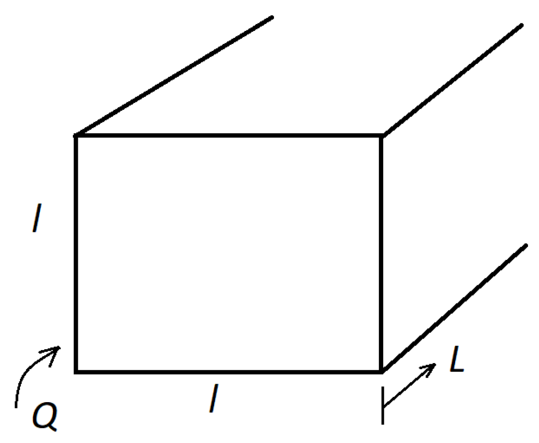
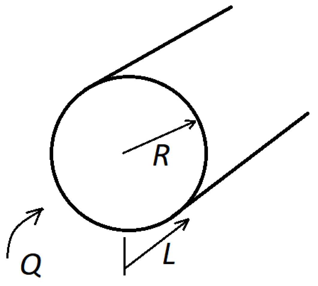
The remainder of the article is structured as follows: Section 2 presents a first idealized modeling of heat transfer over bodies of square and circular sectional areas considering that heat flows towards the body in a uniform way. This is because both the ground platform and the water channel can be considered to have a square or rectangular sectional area, and the edges of the soil platform can suffer erosion, losing their sectional area shape and changing that of the water channel. In extreme cases of erosion of the edges, the soil platform may become a semicircular sectional area with the plant at the center (at the highest point), and similarly, the sectional area of the water channel takes on a semicircular shape due to the material deposited by the erosion of the soil platforms. In Section 3, a mathematical model of heat transfer between bodies with different thermal properties is progressively constructed—emulating the WW arrangement of soil platforms and water channels, alternating in a large extension of cultivation area—to obtain the equations that determine the evolution of the temperatures of the soil platforms and water channels considering thermal energy storage and solar radiation. Section 4 presents an analysis of the feasibility of the experimental implementation of the WWT in crop fields, obtaining a set of parameters that quantify and represent the thermal characteristics of the soil (which itself is a mixture of organic material, clay, stones, roots, and others) and water (which is actually a mixture of water as an aqueous substance, microbes, bacteria, insects, insect material, etc.), and which are used in the equations that determine the evolution of the temperatures of the soil platforms and water channels. The discussion is shown in Section 5, and conclusions are presented in Section 6.

2. Mathematical Model—First Approximation

This section shows the first mathematical model of the WWT based on finite differences; it involves the basic concepts of thermodynamics and heat transfer. Additionally, the criteria and approximations that have been considered for the explication of the WWT are presented.

2.1. Heat Flow on Square-Section Body

Let us consider a square-section body whose sides measure l and L in depth (see Figure 2) over which a heat flow Q is incident uniformly and radially. In this case, it has been assumed—to simplify the problem—that there are no boundary problems, that is, that the temperature at the edges is equal to the middle part of the sides and, furthermore, that L is large enough that the temperature has the same value along the body. This criterion of uniform temperature distribution has been considered assuming that (a) the body temperature is an equivalent representation of the WW temperature because, considering its dimensions and the location of the crops on the soil platform (see Figure 1), the places where boundary conditions occur are far from the crops and are not a subject of study for this paper, and (b) hourly data on ambient temperature and solar radiation are available. Therefore, the behavior of both parameters during the day does not vary greatly, and the homogenization of the temperature within the body occurs between each hour of solar radiation and ambient temperature data readings.

Considering an adiabatic process without heat losses, the square-section body receives a heat flow Q, leading to its temperature rising according to Equation (1) where m is the body mass, $c_p$ is the body’s heat capacity, and $▵T$ is the temperature difference of the body.

$$▵Q=m{c}_p▵T$$

(1)

If we consider that this occurs during a certain time $▵t$, it means that by dividing both sides of Equation (1) by an incremental time $▵t$, it represents a process that changes over time according to Equation (2):

$${\displaystyle \frac{▵Q}{▵t}}=m{c}_p{\displaystyle \frac{▵T}{▵t}}$$

(2)

If $▵t\to 0$, the instantaneous heat flow ${\displaystyle \frac{dQ}{dt}}=\dot{Q}$ is determined according to Equations (3) and (4) through the use of the mathematical concepts of limits and derivatives.

$$\underset{▵t\to 0}{\lim }{\displaystyle \frac{▵Q}{▵t}}=m{c}_p\underset{▵t\to 0}{\lim }{\displaystyle \frac{▵T}{▵t}}$$

(3)

$${\displaystyle \frac{dQ}{dt}}=\dot{Q}=m{c}_p{\displaystyle \frac{dT}{dt}}$$

(4)

In Equation (4), there are two things of interest: the heat flow into the body, which leads to a change in temperature in the time quantified by $\dot{Q}=m{c}_p{\displaystyle \frac{dT}{dt}}$, and the mass m, which, characterized by its density, determines the volume occupied by the body under study.

In this first approximation, the sun is the heat source that allows the process $\dot{Q}=m{c}_p{\displaystyle \frac{dT}{dt}}$. The sun illuminates a given area $A_R$ with a certain intensity called irradiance I according to Equation (5), where I is measured in $W/m^2$ and the area on which solar radiation is incident $A_R$ is measured in $m^2$.

$$\dot{Q}={\displaystyle \frac{dQ}{dt}}=I{A}_R$$

(5)

$A_R$ can be explained as $A_R=C_{R}L$, where $C_R$ is the radiation contour (the equivalent surface that is illuminated by the sun); therefore, Equation (5) is written as Equation (6):

$$\dot{Q}={\displaystyle \frac{dQ}{dt}}=I{A}_R=I{C}_{R}L$$

(6)

The mass m has intrinsic properties of density $\rho$ with $\rho ={\displaystyle \frac{m}{V}}$ and the volume V; therefore, $m=\rho V$. If a uniform sectional area $A_S$ of the square-section body is assumed, then we have that $V=A_{S}L$, $m=\rho A_{S}L$, therefore, as a result, Equation (7) is obtained.

$$m{c}_p{\displaystyle \frac{dT}{dt}}=\rho A_{S}L{c}_p{\displaystyle \frac{dT}{dt}}$$

(7)

Equation (7) is replaced in Equation (4) to relate the interaction between solar radiation and the capture of thermal energy in the square-section body, which is described according to Equations (8)–(10).

$$I{A}_R=\rho A_{S}L{c}_p{\displaystyle \frac{dT}{dt}}$$

(8)

$$I{C}_{R}L=\rho A_{S}L{c}_p{\displaystyle \frac{dT}{dt}}$$

(9)

$$I{C}_R=\rho A_S{c}_p{\displaystyle \frac{dT}{dt}}$$

(10)

Finally, Equation (11) expresses an ideal description of the increase in temperature according to the interaction of the sun with the square-section body.

$${\displaystyle \frac{dT}{dt}}={\displaystyle \frac{I{C}_R}{\rho A_S{c}_p}}$$

(11)

2.2. Heat Flow on Square-Section Body and Convection

In this section, the phenomenon of convection in the square-section body described above is studied (see Figure 3). The convection heat flux $Q_{p_{conv}}$ is defined as $Q_{p_{conv}}=h{A}_{cv}▵T$, where h is the convection coefficient, $A_{cv}$ is the area in which heat is transmitted by convection, and $▵T$ is the temperature difference equal to $▵T=T-T_a$.

In this item, $A_{cv}$ is considered as $A_{cv}=C_{conv}L$, where $C_{conv}$ is the convection contour (line demarcating the convection heat flow area); then, the convection heat flux can be determined according to Equation (12).

$$Q_{p_{conv}}=h{C}_{conv}L▵T$$

(12)

Therefore, the energy balance for a given instant is shown in Equation (13), where ${\dot{Q}}_{al}$ is the thermal energy that is stored in the body, and Equation (14) shows the relationship between the parameters involved in the thermal energy flow process.

$${\dot{Q}}_R-Q_{p_{conv}}={\dot{Q}}_{al}$$

(13)

$$I{C}_{R}L-C_{conv}Lh(T-T_a)=\rho A_{S}L{c}_p{\displaystyle \frac{dT}{dt}}$$

(14)

Let us consider that Equation (14) is a slow process during the day, and consequently, the value of the temperature T throughout the sectional area $A_S$ is the same or evolves in the same way. Furthermore, the concept of derivative by differences according to Equation (15) is introduced, where i is related to time, since this is a process that evolves over time; therefore, the time at a given moment is $T_i$, and the $▵t$ takes a value $T_{i+1}$ as a result of the thermal dynamics present.

$${\displaystyle \frac{dT}{dt}}={\displaystyle \frac{T_{i+1}-T_i}{▵t}}$$

(15)

Then, Equation (14) is rewritten as shown in Equation (16), in which it is considered that if the convection properties do not change over time, that is, $h_i=h$, the parameters are related according to Equation (17).

$$I_i{C}_{R}L-C_{conv}L{h}_i(T_i-T_{a_i})=\rho A_{S}L{c}_p\left[{\displaystyle \frac{T_{i+1}-T_i}{▵t}}\right]$$

(16)

$$I_i{C}_{R}L-C_{conv}Lh(T_i-T_{a_i})=\rho A_{S}L{c}_p\left[{\displaystyle \frac{T_{i+1}-T_i}{▵t}}\right]$$

(17)

Then, by solving for $T_{i+1}$ in Equation (17), Equations (18)–(20) are obtained, where $T_{a_i}$ is the temperature of the environment around the body that changes with time. The unit of time measurement ($▵t$ between readings) is considered as 1 h since the referential data considered was taken from the data reported in NASA Power Access Viewer [10], which provides data at the native sources’ resolution. Primary solar resolution is given as a global $1^{\circ }\times 1^{\circ }$ latitude/longitude grid from CERES SYN1deg, while the meteorological data sources are given as a $1/2^{\circ }\times 5/8^{\circ }$ latitude/longitude grid from GMAO MERRA-2. The solar irradiance is derived from NASA’s GEWEX SRB Release 4-Integrated Product (R4-IP) archive and NASA’s CERES SYN1deg and FLASHFlux projects, and meteorological parameters are derived from NASA’s GMAO MERRA-2 assimilation model and GEOS-IT. MERRA-2 is a version of NASA’s Goddard Earth Observing System (GEOS) Data Assimilation System [11].

$$T_{i+1}-T_i={\displaystyle \frac{▵T}{\rho A_S{c}_p}}\left[I_i{C}_R-C_{conv}h(T_i-T_{a_i})\right]$$

(18)

$$T_{i+1}=T_i+{\displaystyle \frac{▵t}{\rho A_S{c}_p}}\left[I_i{C}_R-C_{conv}h(T_i-T_{a_i})\right]$$

(19)

$$T_{i+1}=T_i\left[1-{\displaystyle \frac{C_{conv}h▵t}{\rho A_S{c}_p}}\right]+{\displaystyle \frac{▵t}{\rho A_S{c}_p}}\left[I_i{C}_R+C_{conv}h{T}_{a_i}\right]$$

(20)

Equation (17) can be generalized considering the change in variables over time and the concept of time discretization (using the subfix i), as shown in Equation (21).

$$I_i{C}_{R_i}-C_{con{v}_i}{h}_i(T_i-T_{a_i})={\rho }_i{A}_{S_i}{c}_{p_i}\left[{\displaystyle \frac{T_{i+1}-T_i}{▵t}}\right]$$

(21)

Until now, in a usual and implicit way, it has been considered that time t advances at a uniform speed, and that the time between readings is the same $▵t$. However, the problem can also be generalized to the fact that the time between measurements $▵t_i$ is variable according to Equation (22), and that for a given period T, there are N readings and they are related according to Equation (23) (see Figure 4).

$$▵t_i=t_{i+1}-t_i$$

(22)

$$T=\sum _{i=1}^{N-1}\left[t_{i+1}-t_i\right]=\sum _{i=1}^{N-1}▵t_i$$

(23)

Also, it is necessary to mention that if the process parameters change over time, they must be explicitly related to time through equations or by recording the value of the parameters in experiments. In the case that approximate or idealized equations are used, the generation of random numbers can be added that emulate the quality and stochastic degradation in the materials.

2.3. Case Studies Assuming Values of the Variables and Generalization of Cases

2.3.1. Case Study 1: Square-Section Body

Considering Figure 2 and considering $C_{conv}=4l$, $A=l^2$, $C_R=4l$ and $▵t=1h=3600$ s in Equation (20), Equations (24) and (25) are obtained, which imply that the temperature increase depends on the width (side) l of the square. Therefore, it is interesting to investigate how the temperature evolves $T_{i+1}$ depending on l, where $▵t=3600$ s (1 h).

$$T_{i+1}=T_i\left[1-{\displaystyle \frac{4lh▵t}{\rho l^2{c}_p}}\right]+{\displaystyle \frac{▵t}{\rho l^2{c}_p}}\left[I_{i}4l+4lh{T}_{a_i}\right]$$

(24)

$$T_{i+1}=T_i\left[1-{\displaystyle \frac{4h▵t}{\rho l{c}_p}}\right]+{\displaystyle \frac{▵t}{\rho l{c}_p}}\left[4I_i+4h{T}_{a_i}\right]$$

(25)

2.3.2. Case Study 2: Circular-Section Body

Let us consider a circular-section body that has radius R and depth L (see Figure 5), where a flow of heat Q impacts its radial and uniform form.

So, we have $C_{conv}=2\pi R$, $A=\pi R^2$, $C_R=2\pi R$ and $▵t=1h=3600s$; therefore, Equations (26) and (27) are obtained.

$$T_{i+1}=T_i\left[1-{\displaystyle \frac{2\pi Rh▵t}{\rho \pi R^2{c}_p}}\right]+{\displaystyle \frac{▵t}{\rho \pi R^2{c}_p}}\left[I_{i}2\pi R+2\pi Rh{T}_{a_i}\right]$$

(26)

$$T_{i+1}=T_i\left[1-{\displaystyle \frac{2h▵t}{\rho R{c}_p}}\right]+{\displaystyle \frac{▵t}{\rho R{c}_p}}\left[2I_i+2h{T}_{a_i}\right]$$

(27)

2.3.3. Generalizing Case Studies

Analyzing case studies 1 and 2, Equation (27) of the circle is possible to write as Equation (28), Equation (25) of the square is possible to write as Equation (29), and, in a general way, this can be written according to Equation (30), where ${\varphi }_f$ is a form factor with dimension $1/m$ and values ${\varphi }_f={\displaystyle \frac{2}{R}}$ for circles, and ${\varphi }_f={\displaystyle \frac{4}{l}}$ for squares.

$$T_{i+1}=T_i\left\{1-\left[{\displaystyle \frac{2}{R}}\right]{\displaystyle \frac{h▵t}{\rho c_p}}\right\}+\left[{\displaystyle \frac{2}{R}}\right]\left\{I_i+h{T}_{a_i}\right\}{\displaystyle \frac{▵t}{\rho c_p}}$$

(28)

$$T_{i+1}=T_i\left\{1-\left[{\displaystyle \frac{4}{l}}\right]{\displaystyle \frac{h▵t}{\rho c_p}}\right\}+\left[{\displaystyle \frac{4}{l}}\right]\left\{I_i+h{T}_{a_i}\right\}{\displaystyle \frac{▵t}{\rho c_p}}$$

(29)

$$T_{i+1}=T_i\left\{1-{\varphi }_f{\displaystyle \frac{h▵t}{\rho c_p}}\right\}+{\varphi }_f\left\{I_i+h{T}_{a_i}\right\}{\displaystyle \frac{▵t}{\rho c_p}}$$

(30)

Equation (30) can be simplified if is considered that ${\varphi }_f=1$, and also that $▵t$ is 1 h and the heat storage material is considered to be water, with which is possible to define a new parameter: the constant of time variation of the volumetric concentration of energy of the substance $\beta$ in ${\displaystyle \frac{°C}{(W/m^3)}}$, according to Equation (31) where the body under study is water and its $\rho$ and $c_p$ values are replaced in the equation (in general, any other substance can be considered by substituting its density and capacity values). So, Equation (30) can be expressed according to Equations (32)–(34), where if $T_i=T_{a_i}$, then heat transfer by convection ceases.

$$\beta ={\displaystyle \frac{▵t}{\rho c_p}}={\displaystyle \frac{1}{\left(1000\right)\left(4.18\right)}}=2.3922\times {10}^{-4}$$

(31)

$$T_{i+1}=T_i\left\{1-\beta h\right\}+\left\{I_i+h{T}_{a_i}\right\}\beta$$

(32)

$$T_{i+1}=T_i-\beta h{T}_i+\beta I_i+\beta h{T}_{a_i}$$

(33)

$$T_{i+1}=T_i+\beta I_i-\beta h(T_i-T_{a_i})$$

(34)

Equation (34) shows that it is possible to determine the evolution of hourly temperature values with addition, multiplication, and parameters characterizing the substance and the heat source.

Using Equation (31), it is possible to determine—in general—the value of $\beta$ for any other substance and with any other value of $▵t$ measured in seconds, which would lead to adjustments in the mathematical model presented in this paper. However, water is one of the fundamental things in agriculture, and the hour is a very useful unit of time for the case study of the WWT.

Case Study No. 1: To visualize thermal energy storage in Equation (30) in the context of the technique under study, a site near Lake Titikaka was considered, whose coordinates are latitude −15.38, longitude −69.95. Hourly data for 23 February 2024 were downloaded from [10]. To visualize the temperature trend of the body, the hourly data of the aforementioned day were replicated for 9 days, ${\varphi }_f=2$, which corresponds to $R=1$ in the circular-section body and $l=2$ in the square-section body, and $h=100$ W/(${\mathrm{m}}^2$ K). The results are shown in Figure 6, where the behavior of the solar irradiation is shown for 9 days, and in Figure 7, where the ambient temperature surrounding the body and the body temperature are shown.

Case Study No. 2:Figure 8 shows the evolution of body temperature and ambient temperature with different ${\varphi }_f$ values. The values considered are 0.25, 0.5, 1, and 2 (already shown in Figure 8). All the curves show a tendency towards establishing an oscillatory state with a maximum value during the day and a minimum value during the night, with a much smaller range than the variation of the ambient temperature during the day and night.

Case Study No. 3: In Figure 9, the evolution of body and ambient temperature over 9 days is shown, with hourly data from 23 February 2024 to 2 March 2024 obtained from [10]. For this case, ${\varphi }_f=2$ was considered.

Case Study No. 4: This case study shows the results obtained when considering a longer period of time for the same location of the crop fields (latitude −15.38, longitude −69.95). Hourly data recorded over 10 years (from 1 January 2010 to 31 December 2019) and obtained from [10] were considered. The environmental variables considered were solar radiation (87,648 data points) and ambient temperature (87,648 data points). Figure 10 shows the hourly behavior of the ambient temperature during the study period (10 years), in which the following values were recorded: a maximum ambient temperature of 23.26 °C, a minimum temperature of −4.57 °C, an average ambient temperature of 9.4038 °C, and a standard deviation of 5.0968 °C. Then, considering a body used as thermal energy storage with ${\varphi }_f=2$ and $h=100$ W/(${\mathrm{m}}^2$ K), the evolution of the body temperature under solar irradiation and ambient temperature is shown in Figure 11 for the study period (10 years), in which the following is recorded: a maximum body temperature equal to 19.6169 °C, a minimum temperature of 2.7880 °C, an average body temperature value equal to 12.0438 °C, and a standard deviation of 2.4610 °C. These results indicate that the average body temperature is 3.64 °C higher than the ambient temperature, that the minimum body temperature is 7.358 °C higher than the ambient temperature, and that this minimum body temperature ensures that the water does not turn into its solid phase (ice). However, of particular interest is that the standard deviation of the body temperature is 48.285% that of the environment. Therefore, it was necessary to plot histograms of both the ambient temperature and the body temperature, which are shown in Figure 12 (histogram of ambient temperature $T_a$) and Figure 13 (histogram of body temperature T). In addition, both histograms were plotted together, as shown in Figure 14, which shows that the body temperature remains more clustered with a difference between the maximum and minimum temperatures of 18.8289 °C compared to the difference between the maximum and minimum ambient temperatures, which is 27.83 °C.

2.4. Modeling of the Experimental Part for the Characterization of the Substance

Furthermore, in Equation (34), it is necessary to quantify $T_i$, $I_i$, and $T_{a_i}$ as values to measure over time; h determines the transfer of heat by convection defined by the media that interact and transfer heat, and h can be invariant over time. Therefore, if there are readings of $T_{i+1}$, $T_i$, $I_i$ and $T_{a_i}$, it is possible to calculate the value of $\beta h$ according to the sequence shown in Equations (35)–(37).

$$T_{i+1}-T_i-\beta I_i=-\beta h(T_i-T_{a_i})$$

(35)

$$\beta h(T_i-T_{a_i})=T_i+I_i-T_{i+1}$$

(36)

$$\beta h={\displaystyle \frac{T_i+I_i-T_{i+1}}{T_i-T_{a_i}}}$$

(37)

$\beta h$ is determined for each pass of i to $i+1$; hence, it can be written as $\beta {\left(h\right)}_{i\to i+1}$, from which we can obtain $N-1$ values to graph during the observation time (graph during their evolution) and/or quantify an average value $\beta {\left(h\right)}_p$ according to Equations (38)–(40).

$$\beta {\left(h\right)}_p={\displaystyle \frac{1}{N-1}}\sum _i^{N-1}{\displaystyle \frac{T_i+I_i-T_{i+1}}{T_i-T_{a_i}}}$$

(38)

$$\beta {\left(h\right)}_p={\displaystyle \frac{1}{N-1}}\sum _i^{N-1}{\displaystyle \frac{(T_i-T_{i+1})+I_i}{(T_i-T_{a_i})}}$$

(39)

$$\beta {\left(h\right)}_p={\displaystyle \frac{1}{N-1}}\sum _i^{N-1}\left\{{\displaystyle \frac{T_i-T_{i+1}}{T_i-T_{a_i}}}+{\displaystyle \frac{I_i}{T_i-T_{a_i}}}\right\}$$

(40)

In Equation (40), it is observed that $T_i-T_{i+1}$ and $T_i-T_{a_i}$ are differentials, and therefore, the result is the same, whether in Celsius or Kelvin degrees.

In case other temperature measurement systems and units are used, the result is the same for the first mathematical component of the summation. A demonstration is made with Fahrenheit degrees, in which the equivalence between Celsius and Fahrenheit degrees is shown in Equation (41), so the temperatures in the times i and $i+1$ are defined according to Equations (42)–(44). Then, by replacing ${\displaystyle \frac{T_i-T_{i+1}}{T_i-T_{a_i}}}$, Equations (45)–(47) are obtained, in which it is shown that the result is the same regardless of the temperature measurement system.

$${\displaystyle \frac{C}{5}}={\displaystyle \frac{F-32}{9}}$$

(41)

$$F_i={\displaystyle \frac{9}{5}}{C}_i+32$$

(42)

$$F_{i+1}={\displaystyle \frac{9}{5}}{C}_{i+1}+32$$

(43)

$$F_{a_i}={\displaystyle \frac{9}{5}}{C}_{a_i}+32$$

(44)

$${\displaystyle \frac{F_i-F_{i+1}}{F_i-F_{a_i}}}={\displaystyle \frac{\frac{9}{5}{C}_i+32-\left\{\frac{9}{5}{C}_{i+1}+32\right\}}{\frac{9}{5}{C}_i+32-\left\{\frac{9}{5}{C}_{a_i}+32\right\}}}$$

(45)

$${\displaystyle \frac{F_i-F_{i+1}}{F_i-F_{a_i}}}={\displaystyle \frac{\frac{9}{5}\left\{C_i-C_{i+1}\right\}}{\frac{9}{5}\left\{C_i-C_{a_i}\right\}}}$$

(46)

$${\displaystyle \frac{F_i-F_{i+1}}{F_i-F_{a_i}}}={\displaystyle \frac{C_i-C_{i+1}}{C_i-C_{a_i}}}$$

(47)

An interesting relationship is ${\displaystyle \frac{I_i}{T_i-T_{a_i}}}$, and the question is how did Incas/pre-Incas perform the reading/measurement of $I_i$? For this and considering the current context of experimentation in crop fields, Equation (40) is rewritten in Equation (48):

$$\beta {\left(h\right)}_p={\displaystyle \frac{1}{N-1}}\sum _i^{N-1}{\displaystyle \frac{T_i-T_{i+1}}{T_i-T_{a_i}}}+{\displaystyle \frac{1}{N-1}}\sum _i^{N-1}{\displaystyle \frac{I_i}{T_i-T_{a_i}}}$$

(48)

Let us assume that—due to their measuring instruments—their experimental readings would have had a proportional error $\gamma$ of $I_i$, that is to say, an experimental value $\left(\gamma I_i\right)$; therefore, Equation (48) is written as Equation (49):

$$\beta {\left(h\right)}_p={\displaystyle \frac{1}{N-1}}\sum _i^{N-1}{\displaystyle \frac{T_i-T_{i+1}}{T_i-T_{a_i}}}+{\displaystyle \frac{1}{N-1}}\sum _i^{N-1}{\displaystyle \frac{\left(\gamma I_i\right)}{T_i-T_{a_i}}}$$

(49)

Then, based on measurements, it is possible to determine the value of that factor $\gamma$ with the purpose that Equation (48) can predict the behavior of temperatures; that is to say, if Equation (40) is written as Equation (50), ${\displaystyle \frac{1}{\gamma }}$ can also be used to compensate for the equivalence between units of measurement of irradiation in the numerator $I_i$ and the temperatures $T_i-T_{a_i}$ in the denominator.

$$\beta {\left(h\right)}_p={\displaystyle \frac{1}{N-1}}\sum _i^{N-1}{\displaystyle \frac{T_i-T_{i+1}}{T_i-T_{a_i}}}+\left\{{\displaystyle \frac{1}{\gamma }}\right\}{\displaystyle \frac{1}{N-1}}\sum _i^{N-1}{\displaystyle \frac{\left(\gamma I_i\right)}{T_i-T_{a_i}}}$$

(50)

For this, they had to take measurements in experimental facilities and then assume different values of ${\displaystyle \frac{1}{\gamma }}$, and then the respective calculations were carried out to determine the experimental installation, which gives values equal to those calculated (see the flow diagram in Figure 15. To perform these calculations, the Incas/pre-Incas had a recording and calculating system, such as quipu or yupana, with which they could perform addition and multiplication with calculation procedures such as those reported in [12].

If the Incas/pre-Incas were able to determine ${\displaystyle \frac{1}{\gamma }}$—as archaeological evidence confirms—then they knew how to correct the radiation measurement $I_i$ by making an adjustment to the instrument (if it had been possible to make with the instrument) or an adjustment to the measurement, obtaining Equation (51).

$$T_{i+1}=T_i+{\displaystyle \frac{\left(\gamma I_i\right)}{\gamma }}-\beta {\left(h\right)}_p(T_i-T_{a_i})$$

(51)

Considering that many readings have been taken such that it can be assumed that $\beta {\left(h\right)}_p\approx \beta h$, Equation (51) is possible to write as Equation (52):

$$T_{i+1}=T_i+{\displaystyle \frac{\left(\gamma I_i\right)}{\gamma }}-\beta h(T_i-T_{a_i})$$

(52)

Then, for practical purposes, if is considered that $I_{e_i}=\gamma I_i$ is the wrong reading of the irradiation, ${\gamma }^{\prime }={\displaystyle \frac{1}{\gamma }}$ is the irradiation measurement correction factor, and $\sigma =\beta h$ is the convection factor, so Equation (52) can be written as shown in Equation (53) in which addition, subtraction, and multiplication operations are observed, which were known to the Incas/pre-Incas.

$$T_{i+1}=T_i+{\gamma }^{\prime }{T}_{e_i}-\sigma (T_i-T_{a_i})$$

(53)

2.5. Generalization of Shapes

Previously, we obtained Equation (54) (see Equation (30)), which is rewritten as Equation (55), where patterns of $I_i$ and $T_{a_i}$ can be taken into account, with the same initial condition $T_i$ but varying h and ${\varphi }_f$ for both case studies of bodies with circular and square sections.

$$T_{i+1}=T_i\left\{1-{\varphi }_f{\displaystyle \frac{h▵t}{\rho c_p}}\right\}+{\varphi }_f\left\{I_i+h{T}_{a_i}\right\}{\displaystyle \frac{▵t}{\rho c_p}}$$

(54)

$$T_{i+1}=T_i\left\{1-{\varphi }_f\beta h\right\}+{\varphi }_f\left\{I_i+h{T}_{a_i}\right\}\beta$$

(55)

Also, the same condition can be considered for $I_i$, $T_{a_i}$, $T_i$ and h. To observe its behavior with different values of ${\varphi }_f$ (square- and circular-section bodies), that is, when writing Equation (55) applied to the circular-section body, Equation (56) is obtained and applied to the square-section body, and Equation (57) is also obtained:

$$T_{i+1}^{\circ }=T_i\left\{1-{\varphi }_f^{\circ }\beta h^{\circ }\right\}+{\varphi }_f^{\circ }\left\{I_i+h^{\circ }{T}_{a_i}\right\}\beta$$

(56)

$$T_{i+1}^{\square }=T_i\left\{1-{\varphi }_f^{\square }\beta h^{\square }\right\}+{\varphi }_f^{\square }\left\{I_i+h^{\square }{T}_{a_i}\right\}\beta$$

(57)

Then, the difference in temperatures at any time $i+1$ can be determined by Equations (58) and (59):

$$T_{i+1}^{\circ }-T_{i+1}^{\square }=T_i\beta \left\{{\varphi }_f^{\circ }{h}^{\circ }-{\varphi }_f^{\square }{h}^{\square }\right\}+\beta T_{a_i}\left\{{\varphi }_f^{\circ }{h}^{\circ }-{\varphi }_f^{\square }{h}^{\square }\right\}+I_i\beta \left\{{\varphi }_f^{\circ }-{\varphi }_f^{\square }\right\}$$

(58)

$$T_{i+1}^{\circ }-T_{i+1}^{\square }=\beta (T_i+T_{a_i})\left\{{\varphi }_f^{\circ }{h}^{\circ }-{\varphi }_f^{\square }{h}^{\square }\right\}+I_i\beta \left\{{\varphi }_f^{\circ }-{\varphi }_f^{\square }\right\}$$

(59)

If the same convection properties are considered, that is, $h^{\circ }=h^{\square }=h^{\circ \square }$, Equations (60) and (61) are obtained, with which different curves can be constructed, considering ${\varphi }_f^{\circ }$ and ${\varphi }_f^{\square }$, which are applicable for the initial moment of each morning when both have the same temperature and the sun begins to radiate over the crop fields. The beginning of the day would be a uniform and equal set point.

$$T_{i+1}^{\circ }-T_{i+1}^{\square }=\beta h^{\circ \square }(T_i+T_{a_i})\left\{{\varphi }_f^{\circ }-{\varphi }_f^{\square }\right\}+I_i\beta \left\{{\varphi }_f^{\circ }-{\varphi }_f^{\square }\right\}$$

(60)

$$T_{i+1}^{\circ }-T_{i+1}^{\square }=\beta \left\{h^{\circ \square }(T_i+T_{a_i})+I_i\right\}\left\{{\varphi }_f^{\circ }-{\varphi }_f^{\square }\right\}$$

(61)

3. Mathematical Model—Second Approximation

The typical configuration of the WWT is the alternative placement of soil and water, which have different thermal behavior in energy storage and thermal energy exchange between themselves and between them and the air. This section shows a mathematical model that shows the behavior over time of the soil and water temperatures conditioned by the temperature of the environment, the solar radiation that influences both, and the temperature of the subsoil (located below the soil–water arrangement that exists on the surface of the crop field).

Let us take the general heat equation described in Equation (62), where $\rho$ is the density, c is the specific heat capacity, and k is the thermal conductivity of the substance, representing the variation of temperature in space and time due to the entry of heat or the generation of heat inside the substance.

$$Q+{\displaystyle \frac{{\partial }^{2}T}{\partial r^2}}={\displaystyle \frac{\rho c}{k}}{\displaystyle \frac{\partial T}{\partial t}}$$

(62)

An equivalent temperature is considered for the temperature change that occurs in the medium, and, therefore, there is no temperature variation inside the substance, leading to Equation (63) since the body would behave as a point element in which there would be no temperature differences between the outside and inside of the body. That is to say, a body whose temperature is uniform at all points is considered. In the case of the WWT, temperature control is performed every hour, enough time for the temperature variations within each part of the WW to be considered uniform and stable.

$$Q={\displaystyle \frac{\rho c}{k}}{\displaystyle \frac{\partial T}{\partial t}}$$

(63)

The concept of the derivative can be represented using incrementals by Equation (64), which is substituted into Equation (63) to obtain Equations (65) and (66), where $\alpha$ is the diffusivity of the substance ($\alpha ={\displaystyle \frac{k}{\rho c}}$) under study.

$${\displaystyle \frac{\partial T}{\partial t}}={\displaystyle \frac{T_{(t+1)}-T_t}{▵t}}$$

(64)

$${\displaystyle \frac{T_{(t+1)}-T_t}{▵t}}={\displaystyle \frac{k}{\rho c}}Q=\alpha Q$$

(65)

$$T_{(t+1)}=T_t+▵t{\displaystyle \frac{k}{\rho c}}Q=T_t+▵t\alpha Q$$

(66)

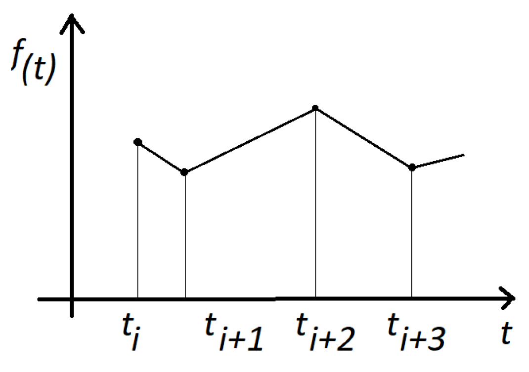
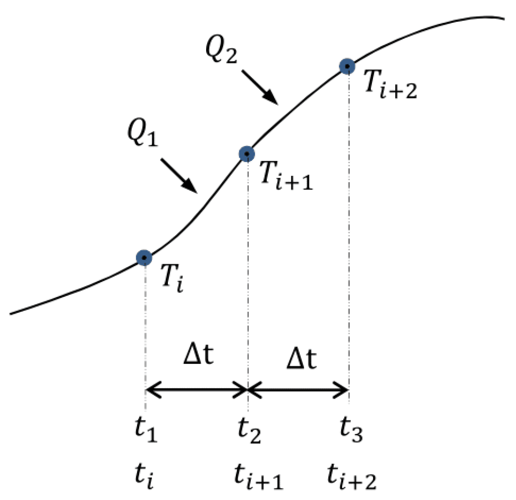
The energy flow readings and temperature readings are considered to be discrete with a certain time interval between readings $▵t$ that is uniform for all the process; therefore, $t_1=t_1$, $t_2=▵t$, $t_3=t_1+2▵t$, $t_4=t_1+3▵t$ and so on. Additionally, during each time interval $▵t$, there would be an input of thermal energy specific to that interval, that is, $Q_1$, $Q_2$, $Q_3$, and so on, as shown in Figure 16. In this manner, Equation (66) can be discretized and expressed as Equation (67), where $i=1,2,3,\dots$ is the time interval number and $Q_i$ is the net heat that is captured by the substance.

$$T_{(i+1)}=T_i+i\alpha Q_i▵t$$

(67)

In the Section 3.1 of this paper, it is assumed that $\alpha$ is a constant value, i.e., it does not change over time since $\rho$, c and k do not vary. This is given that the mathematical model developed is considered as an approximation to the description of the real process.

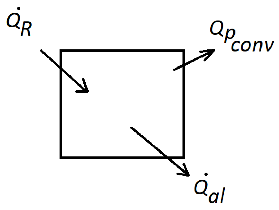
3.1. A Body with Convection Losses

Since each period between readings is listed with i, the heat $Q_i$ is equal to the heat of solar radiation $Q_{R_i}$ minus convection heat $Q_{c_i}$, which is energy that is returned to the environment, as can be seen in Equations (68) and (69), where $h_i$ is the convection coefficient of the material, $T_i$ the body temperature, $T_{a_i}$ is the temperature of the environment around the body, and A is the area through which thermal energy flows by convection. Equation (67) under these considerations is written as Equation (70).

$$Q_i=Q_{R_i}-Q_{c_i}$$

(68)

$$Q_{c_i}=h_{i}A(T_i-T_{a_i})$$

(69)

$$T_{(i+1)}=T_i+i\alpha ▵t\left[Q_{R_i}-h_{i}A(T_i-T_{a_i})\right]$$

(70)

This one-body behavior will then—in the following items—be extended to two bodies: one will represent the cultivation soil that has water on both sides, and the other will represent the water. Together, they represent a thermal energy storage system intended for agriculture called WW, which has been used for centuries and is becoming important today as a measure to counteract global warming and climate change.

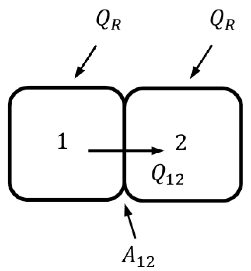
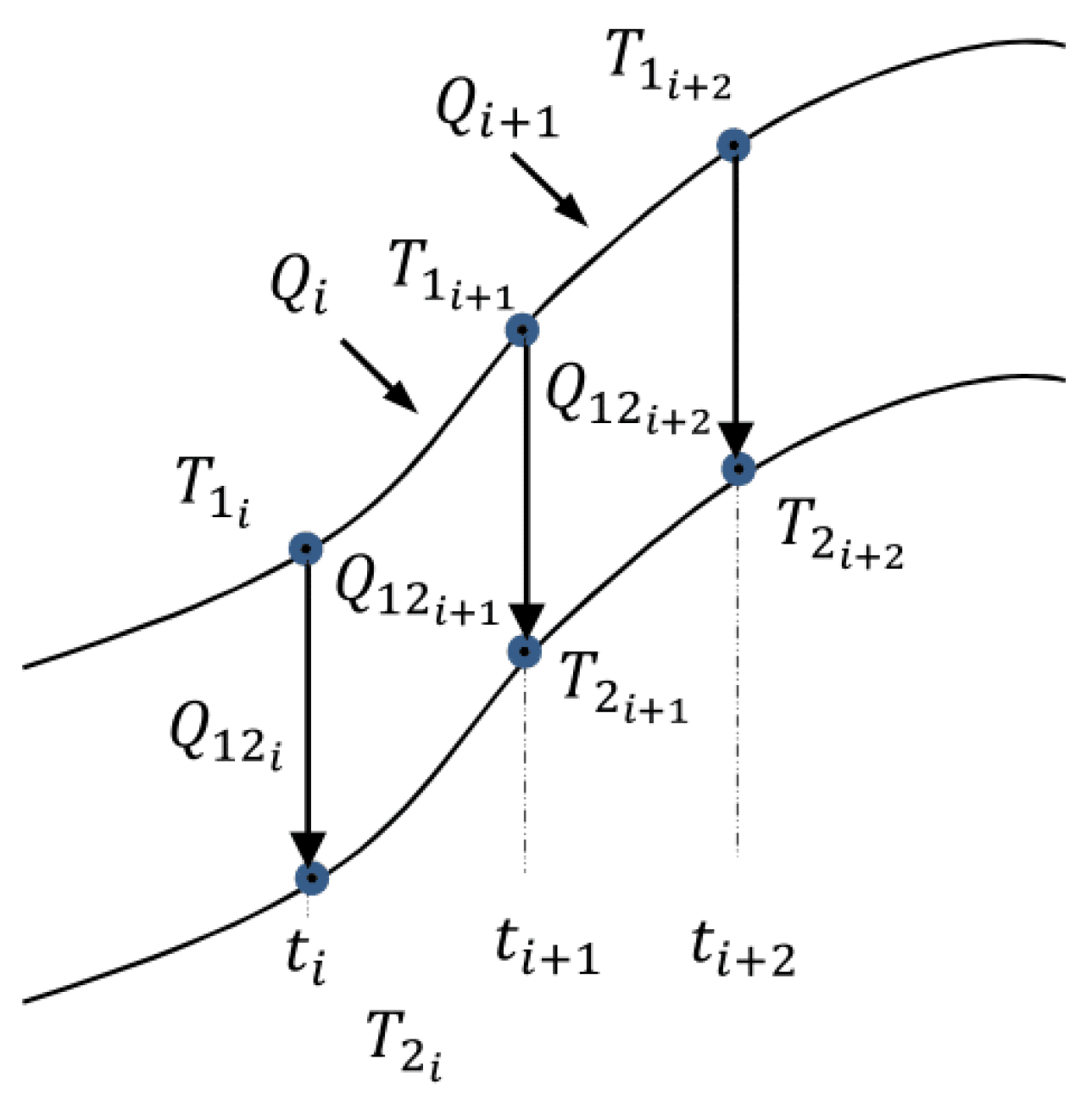
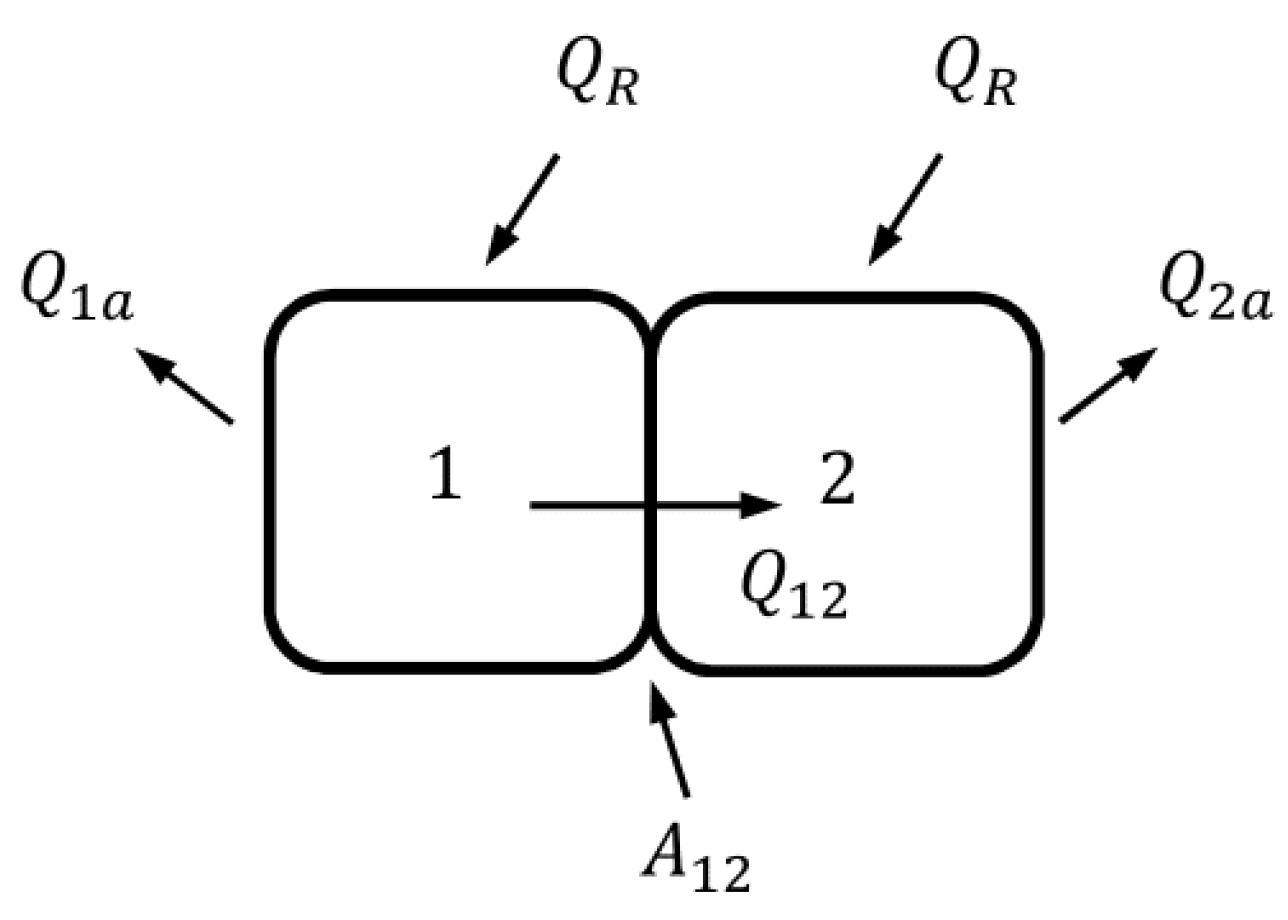
3.2. Two Bodies in Contact and Different Thermal Properties—Without Convection

Figure 17 and Figure 18 show the flow of thermal energy by radiation and conduction and the evolution of temperatures that lead to obtaining Equations (71) and (72), where it is understood that $Q_{1_i}$ and $Q_{2_i}$ are the heat values that affect bodies 1 and 2, respectively.

$$T_{1_{(i+1)}}=T_{1_i}+i{\alpha }_1▵t{Q}_{1_i}$$

(71)

$$T_{2_{(i+1)}}=T_{2_i}+i{\alpha }_2▵t{Q}_{2_i}$$

(72)

The heat flow by conduction $Q_c=-kA▵T/L$ applied to the case under study is obtained by Equation (73).

$$Q_{{12}_i}=-k_{12}{A}_{12}{\displaystyle \frac{T_{1_i}-T_{2_i}}{L_{12}}}$$

(73)

Thermodynamics states that heat naturally moves from an object with a higher temperature to one with a lower temperature, resulting in the flow of thermal energy. Assuming that the heat by conduction goes from body 1 to 2, Equation (74) is obtained.

$$Q_{1_i}=Q_{R_i}+Q_{{12}_i}$$

(74)

Furthermore, considering that the radiation $Q_R$ that both bodies 1 and 2 receive is equal, then Equations (75) and (76) are obtained, where $k_{12}$ is the thermal conductivity coefficient that allows the passage of thermal energy from body 1 to 2; $A_{12}$ is the equivalent area through which the flow of thermal energy occurs between bodies 1 and 2 (or area of interaction by conduction between bodies 1 and 2); and $L_{12}$ is the equivalent distance (distance between centers of mass) between bodies 1 and 2. It is assumed that the rest of the surfaces do not intervene in the process, that is, they are adiabatic.

$$Q_{1_i}=Q_{R_i}-k_{12}{A}_{12}{\displaystyle \frac{T_{1_i}-T_{2_i}}{L_{12}}}$$

(75)

$$Q_{2_i}=Q_{R_i}+k_{12}{A}_{12}{\displaystyle \frac{T_{1_i}-T_{2_i}}{L_{12}}}$$

(76)

So, by rearranging Equations (75) and (76), Equations (77) and (78) are obtained, which allow us to determine the temperatures $T_{1_{(i+1)}}$ and $T_{2_{(i+1)}}$.

$$T_{1_{(i+1)}}=T_{1_i}+i{\alpha }_1▵t\left[Q_{R_i}-k_{12}{A}_{12}{\displaystyle \frac{T_{1_i}-T_{2_i}}{L_{12}}}\right]$$

(77)

$$T_{2_{(i+1)}}=T_{2_i}+i{\alpha }_2▵t\left[Q_{R_i}+k_{12}{A}_{12}{\displaystyle \frac{T_{1_i}-T_{2_i}}{L_{12}}}\right]$$

(78)

3.3. Two Bodies in Contact with Different Thermal Properties and Convection with the Air

It is considered that $Q_{a_1}$ and $Q_{a_2}$ are the convection losses of each body, as shown in Figure 19, and whose mathematical expressions are shown in Equations (79) and (80). Then, the heat fluxes in each period i are shown in Equations (81) and (82).

$$Q_{a_1}=h_{1_i}{A}_{a_i}\left(T_{1_i-T_{a_i}}\right)$$

(79)

$$Q_{a_2}=h_{2_i}{A}_{2_i}\left(T_{2_i-T_{a_i}}\right)$$

(80)

$$Q_{1_i}=Q_{R_i}-k_{12}{A}_{12}{\displaystyle \frac{T_{1_i}-T_{2_i}}{L_{12}}}-h_{1_i}{A}_{1a}\left(T_{1_i-T_{a_i}}\right)$$

(81)

$$Q_{2_i}=Q_{R_i}+k_{12}{A}_{12}{\displaystyle \frac{T_{1_i}-T_{2_i}}{L_{12}}}-h_{2_i}{A}_{2a}\left(T_{1_i-T_{a_i}}\right)$$

(82)

Therefore, by rearranging Equations (81) and (82), (83) and (84) are obtained, which allow us to determine the temperatures $T_{1_{(i+1)}}$ and $T_{2_{(i+1)}}$.

$$T_{1_{(i+1)}}=T_{1_i}+i{\alpha }_1▵t\left\{Q_{R_i}-k_{12}{A}_{12}{\displaystyle \frac{T_{1_i}-T_{2_i}}{L_{12}}}-h_{1_i}{A}_{1a}\left(T_{1_i-T_{a_i}}\right)\right\}$$

(83)

$$T_{2_{(i+1)}}=T_{2_i}+i{\alpha }_2▵t\left\{Q_{R_i}-k_{12}{A}_{12}{\displaystyle \frac{T_{1_i}-T_{2_i}}{L_{12}}}-h_{2_i}{A}_{2a}\left(T_{2_i-T_{a_i}}\right)\right\}$$

(84)

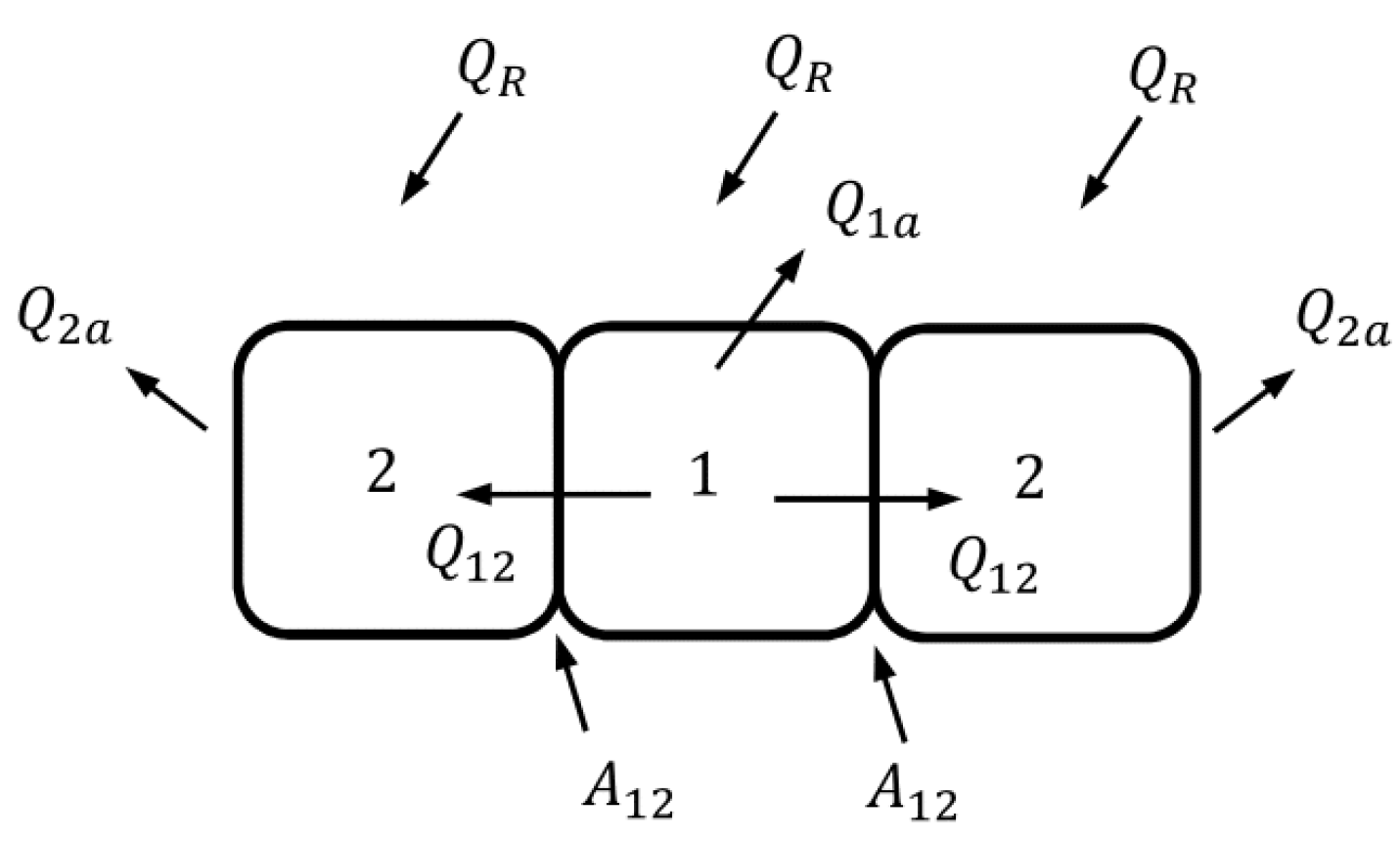
3.4. Three Bodies in Contact with Different Thermal Properties and Convection with the Air

Figure 20 shows an arrangement of bodies 1 and 2, which are considered to be of different nature (they are different material substances); for example, in the case of a WW, the materials are soil and water. Under these considerations and continuing the same conduction and convection procedure, Equations (85) and (86) are obtained.

$$T_{1_{(i+1)}}=T_{1_i}+i{\alpha }_1▵t\left\{Q_{R_i}-2k_{12}{A}_{12}{\displaystyle \frac{T_{1_i}-T_{2_i}}{L_{12}}}-h_{1_i}{A}_{1a}\left(T_{1_i-T_{a_i}}\right)\right\}$$

(85)

$$T_{2_{(i+1)}}=T_{2_i}+i{\alpha }_2▵t\left\{Q_{R_i}-2k_{12}{A}_{12}{\displaystyle \frac{T_{1_i}-T_{2_i}}{L_{12}}}-h_{2_i}{A}_{2a}\left(T_{2_i-T_{a_i}}\right)\right\}$$

(86)

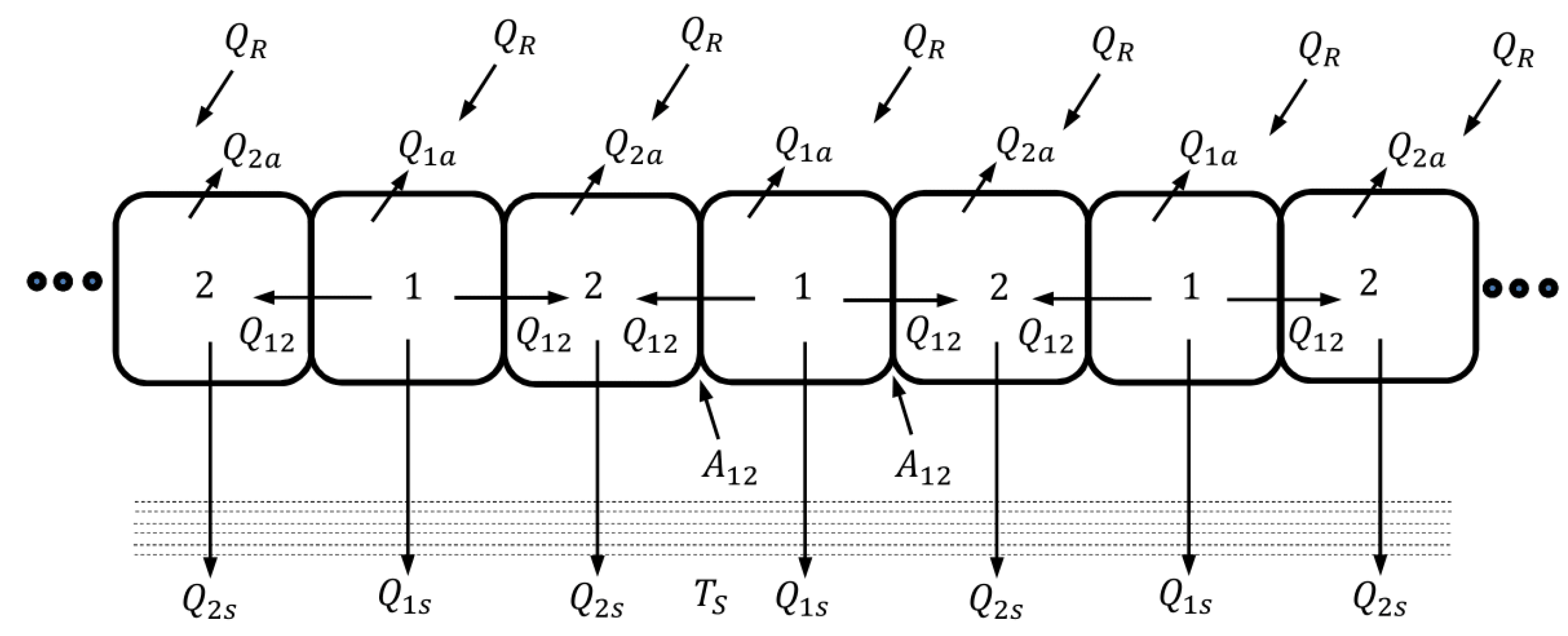
3.5. Many Bodies in Contact with Different Thermal Properties and Convection with the Air and Conduction with Soil

This is the most general case, and as shown in Figure 21, the arrangement consists of many bodies 1 and 2. In addition, there is interaction by conduction with the ground, which is described according to Equations (87) and (88). Under these considerations and continuing the same conduction and convection procedure, Equations (89) and (90) are obtained.

$$Q_{1s}=-k_{1s}{A}_{1s}{\displaystyle \frac{T_{1i}-T_s}{L_{1s}}}$$

(87)

$$Q_{2s}=-k_{2s}{A}_{2s}{\displaystyle \frac{T_{2i}-T_s}{L_{2s}}}$$

(88)

$$\begin{array}{c}{T}_{1_{(i+1)}}=T_{1_i}+i{\alpha }_1▵t\left\{Q_{R_i}-2k_{12}{A}_{12}{\displaystyle \frac{T_{1_i}-T_{2_i}}{L_{12}}}-h_{1_i}{A}_{1a}\left(T_{1_i-T_{a_i}}\right)\right\}\hfill \\ \hspace{1em}\hspace{1em}\hspace{1em}\hspace{1em}\hspace{1em}\hspace{1em}\hspace{1em}\hspace{1em}\hspace{1em}\hspace{1em}\hspace{1em}\hspace{1em}\hspace{1em}\hspace{1em}\hspace{1em}\hspace{1em}\hspace{1em}\hspace{1em}\hspace{1em}\hspace{1em}\hspace{1em}-i{\alpha }_1▵t\left\{k_{1s}{A}_{1s}{\displaystyle \frac{T_{1i}-T_s}{L_{1s}}}\right\}\hfill \end{array}$$

(89)

$$\begin{array}{c}{T}_{2_{(i+1)}}=T_{2_i}+i{\alpha }_2▵t\left\{Q_{R_i}-2k_{12}{A}_{12}{\displaystyle \frac{T_{1_i}-T_{2_i}}{L_{12}}}-h_{2_i}{A}_{2a}\left(T_{2_i-T_{a_i}}\right)\right\}\hfill \\ \hspace{1em}\hspace{1em}\hspace{1em}\hspace{1em}\hspace{1em}\hspace{1em}\hspace{1em}\hspace{1em}\hspace{1em}\hspace{1em}\hspace{1em}\hspace{1em}\hspace{1em}\hspace{1em}\hspace{1em}\hspace{1em}\hspace{1em}\hspace{1em}\hspace{1em}\hspace{1em}\hspace{1em}-i{\alpha }_2▵t\left\{k_{2s}{A}_{2s}{\displaystyle \frac{T_{2i}-T_s}{L_{2s}}}\right\}\hfill \end{array}$$

(90)

Therefore, what has been shown in (89) and (90) means that the thermal behavior has been generalized: as long as there are many bodies 1 and 2, the thermal behavior of bodies 1 and 2, whatever their location in relation to the crops, will be the same.

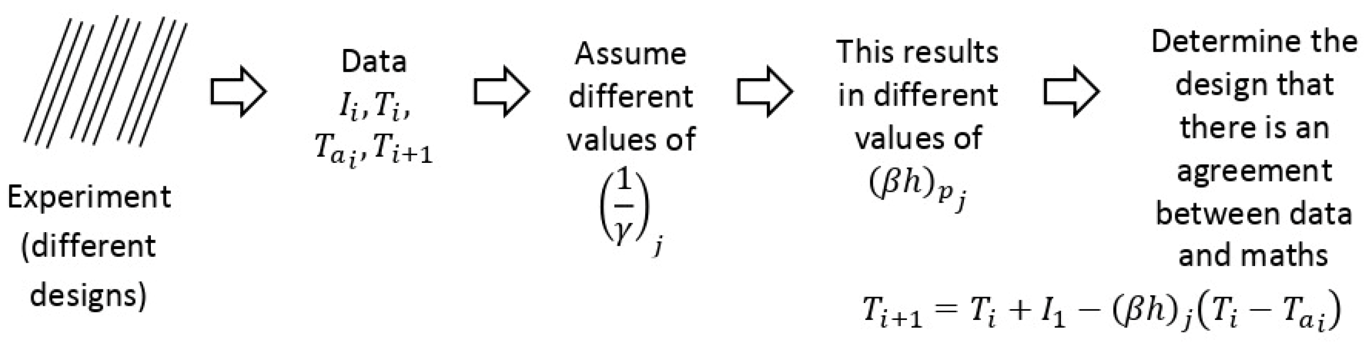
4. Feasibility of Experimental Implementation

Equation (89) of $T_{1_{(i+1)}}$ is an expression that depends on the previous temperature values and solar radiation, as shown in Equation (91).

$$\begin{array}{c}{T}_{1_{(i+1)}}=T_{1_i}-(i▵t)\left\{{\alpha }_1\left\{{\displaystyle \frac{2k_{12}{A}_{12}}{L_{12}}}+h_{1_i}{A}_{1a}+{\displaystyle \frac{k_{1s}{A}_{1s}}{L_{1s}}}\right\}\right\}{T}_{1_i}+\\ (i▵t)\left\{{\displaystyle \frac{{\alpha }_{1}2k_{12}{A}_{12}}{L_{12}}}\right\}{T}_{2_i}+(i▵t)\left\{{\alpha }_1{h}_{1_i}{A}_{1a}\right\}{T}_{a_i}+\\ (i▵t)\left\{{\displaystyle \frac{{\alpha }_1{k}_{1s}{A}_{1s}}{L_{1s}}}\right\}{T}_s+{\alpha }_1(i▵t)Q_{R_i}\end{array}$$

(91)

Equation (91) can be simplified to Equations (92)–(96), which contain constant coefficients since the properties of the materials and geometries are conserved.

$$T_{1_{(i+1)}}=T_{1_i}-(i▵t){\xi }_1{T}_{1_i}+(i▵t){\xi }_2{T}_{2_i}+(i▵t){\xi }_3{T}_{a_i}+(i▵t){\xi }_4{T}_s+{\alpha }_1(i▵t)Q_{R_i}$$

(92)

$${\xi }_1={\alpha }_1\left\{{\displaystyle \frac{2k_{12}{A}_{12}}{L_{12}}}+h_{1_i}{A}_{1a}+{\displaystyle \frac{k_{1s}{A}_{1s}}{L_{1s}}}\right\}$$

(93)

$${\xi }_2={\displaystyle \frac{{\alpha }_{1}2k_{12}{A}_{12}}{L_{12}}}$$

(94)

$${\xi }_3={\alpha }_1{h}_{1_i}{A}_{1a}$$

(95)

$${\xi }_4={\displaystyle \frac{{\alpha }_1{k}_{1s}{A}_{1s}}{L_{1s}}}$$

(96)

Finally, Equation (92), which is used to determine the temperature evolution in body 1, can be expressed as shown in Equation (97).

$$T_{1_{(i+1)}}=(1-i▵t{\xi }_1)T_{1_i}+(i▵t){\xi }_2{T}_{2_i}+(i▵t){\xi }_3{T}_{a_i}+(i▵t){\xi }_4{T}_s+{\alpha }_1(i▵t)Q_{R_i}$$

(97)

For body 2, a procedure similar to that carried out with Equation (89) is carried out with Equation (90) and whose ordered expression is shown in Equation (98), which depends on the previous values of temperature and solar radiation.

$$\begin{array}{c}{T}_{2_{(i+1)}}=T_{2_i}-(i▵t)\left\{{\alpha }_2\left\{{\displaystyle \frac{2k_{12}{A}_{12}}{L_{12}}}+h_{2_i}{A}_{2a}+{\displaystyle \frac{k_{2s}{A}_{2s}}{L_{2s}}}\right\}\right\}{T}_{2_i}+\\ (i▵t)\left\{{\displaystyle \frac{{\alpha }_{2}2k_{12}{A}_{12}}{L_{12}}}\right\}{T}_{1_i}+(i▵t)\left\{{\alpha }_2{h}_{2_i}{A}_{2a}\right\}{T}_{a_i}+\\ (i▵t)\left\{{\displaystyle \frac{{\alpha }_2{k}_{2s}{A}_{2s}}{L_{2s}}}\right\}{T}_s+{\alpha }_2(i▵t)Q_{R_i}\end{array}$$

(98)

Equation (98) can be simplified to Equations (99)—(103), where coefficients are used that contain the properties of the materials and that, together with the geometries, are preserved.

$$T_{2_{(i+1)}}=(1-i▵t{\gamma }_1)T_{2_i}+(i▵t){\gamma }_2{T}_{1_i}+(i▵t){\gamma }_3{T}_{a_i}+(i▵t){\gamma }_4{T}_s+{\alpha }_2(i▵t)Q_{R_i}$$

(99)

$${\gamma }_1={\alpha }_2\left\{{\displaystyle \frac{2k_{12}{A}_{12}}{L_{12}}}+h_{2_i}{A}_{2a}+{\displaystyle \frac{k_{2s}{A}_{2s}}{L_{2s}}}\right\}$$

(100)

$${\gamma }_2={\displaystyle \frac{{\alpha }_{2}2k_{12}{A}_{12}}{L_{12}}}$$

(101)

$${\gamma }_3={\alpha }_2{h}_{2_i}{A}_{2a}$$

(102)

$${\gamma }_4={\displaystyle \frac{{\alpha }_2{k}_{2s}{A}_{2s}}{L_{2s}}}$$

(103)

In both Equations (97) and (99), there are five coefficients to be determined: those in Equation (97) are ${\xi }_1$, ${\xi }_2$, ${\xi }_3$, ${\xi }_4$, and ${\alpha }_1$, while those in Equation (99) are ${\gamma }_1$, ${\gamma }_2$, ${\gamma }_3$, ${\gamma }_4$, and ${\alpha }_2$. If temperature and solar radiation data are taken, the values of the coefficients can be determined. Therefore, as there are 5 coefficients to be determined, at least 5 readings are required; then, Equation (97) is written in the form shown in Equation (104) to determine the change in the temperature readings.

$$T_{1_{(i+1)}}-T_{1_i}=-(i▵t){\xi }_1{T}_{1_i}+(i▵t){\xi }_2{T}_{2_i}+(i▵t){\xi }_3{T}_{a_i}+(i▵t){\xi }_4{T}_s+{\alpha }_1(i▵t)Q_{R_i}$$

(104)

On the right side of Equation (104), it can be observed that the expression $i▵t$ is present in all the components, which makes it feasible to take it to the left side of the equality, and then, the equations to determine the value of the coefficients $\xi$ and $\gamma$ with field readings are written as Equations (105) and (106).

$$-{\xi }_1{T}_{1_i}+{\xi }_2{T}_{2_i}+{\xi }_3{T}_{a_i}+{\xi }_4{T}_s+{\alpha }_1{Q}_{R_i}={\displaystyle \frac{T_{1_{(i+1)}}-T_{1_i}}{i▵t}}$$

(105)

$$-{\gamma }_1{T}_{2_i}+{\gamma }_2{T}_{1_i}+{\gamma }_3{T}_{a_i}+{\gamma }_4{T}_s+{\alpha }_2{Q}_{R_i}={\displaystyle \frac{T_{2_{(i+1)}}-T_{2_i}}{i▵t}}$$

(106)

Once the coefficients $\xi$, $\gamma$, ${\alpha }_1$, and ${\alpha }_2$ have been determined, the values of the other variables involved can be deduced.

5. Discussion

The Inca and pre-Inca cultures have long been considered outstanding for their technological achievements, including high-altitude agriculture. As written above, it should be considered that understanding their technologies and techniques involves a mixture of physical principles and high mathematics that can be conducted with simple operations and test crops for adjustments of local crop yield parameters. It was essential to master the principles of thermal energy storage and to know how to apply them. In the specific case study of this paper, sustainable thermal energy storage and its application were studied in high Andean areas near Lake Titikaka, territories dominated by the low temperatures that occur above 3800 m above sea level, which were converted into productive lands that have allowed the establishment of populations and cultures for many centuries up to the present day.

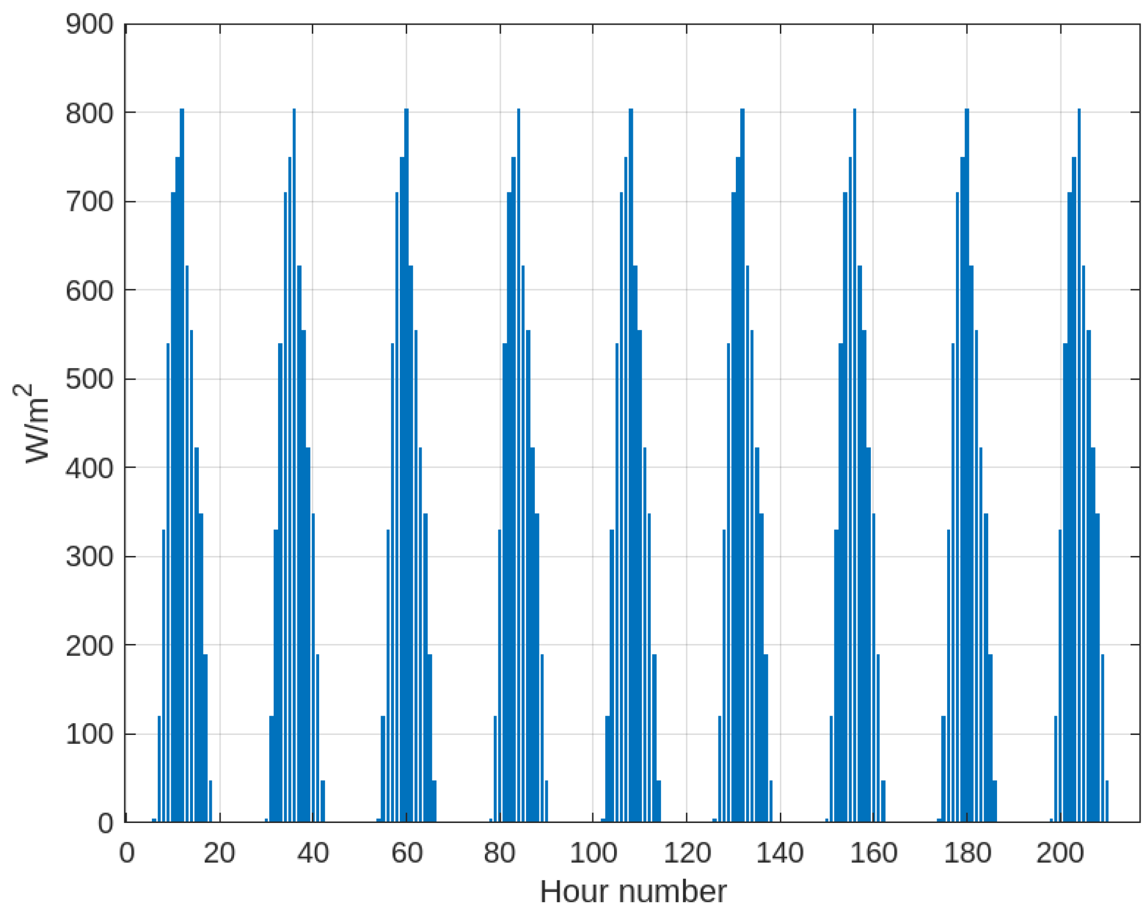
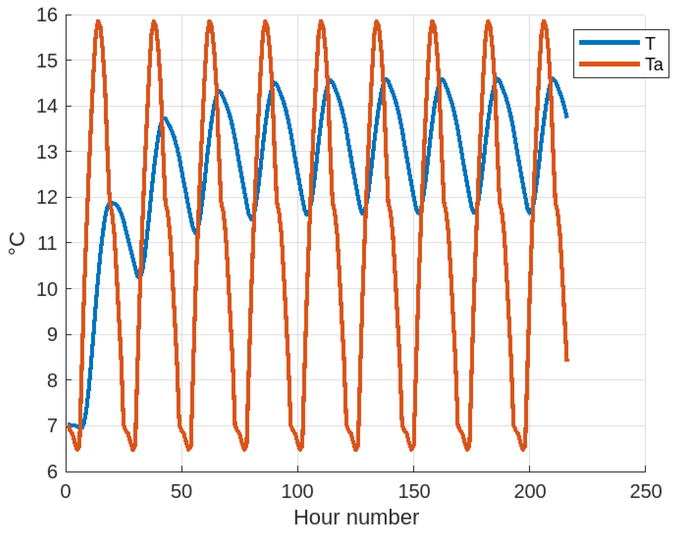
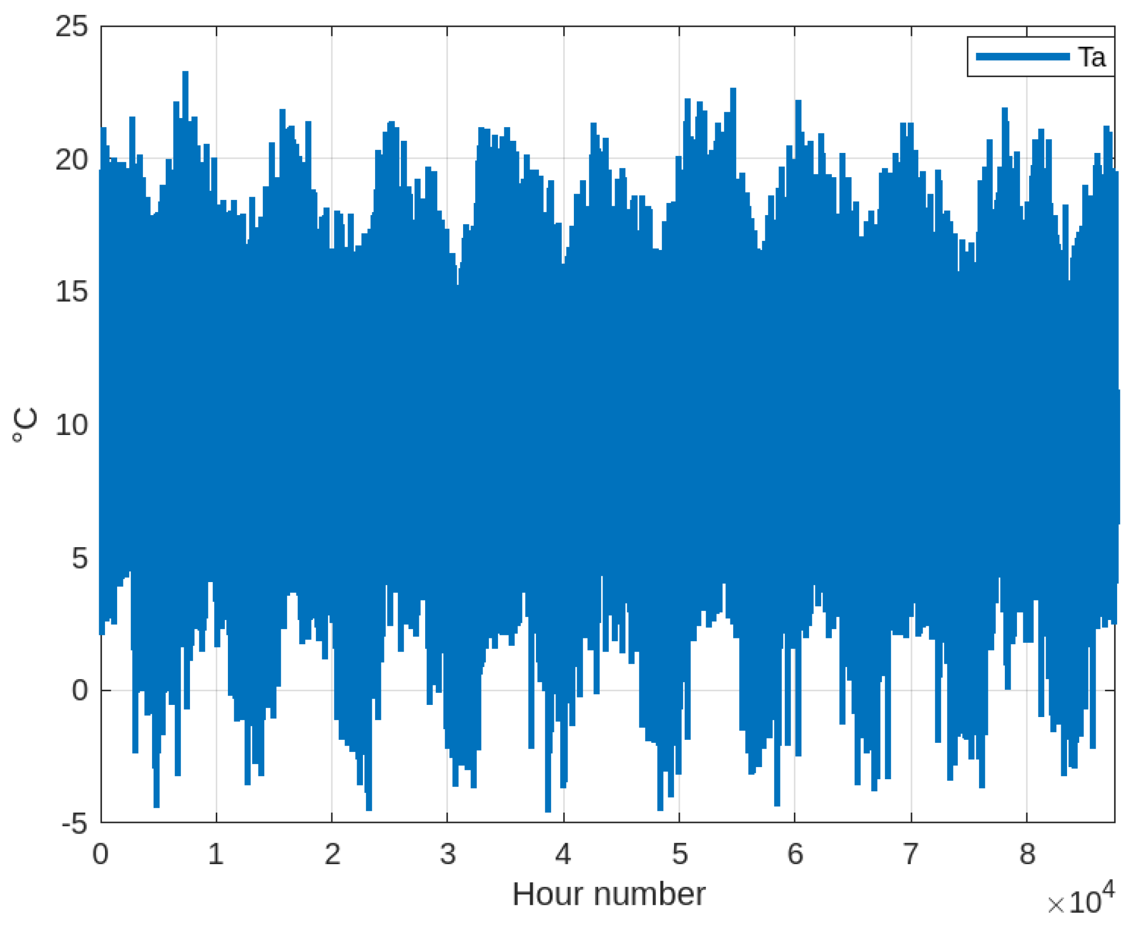
Analyzing the data shown in Figure 7 in which the ambient temperature and solar irradiation data of a specific day (23 February 2024) have been considered as a reference for the calculation of the body temperature trend, it is found that from an initial body temperature equal to the ambient temperature of the first hour of the data, there is an increase to a steady state whose maximum body temperature is 14.59 °C and minimum body temperature is 11.61 °C, which is a body temperature difference of 2.98 °C. Meanwhile, the maximum ambient temperature is 15.86 °C and the minimum ambient temperature is 6.47 °C, which is an ambient temperature difference of 9.39 °C. Then, the temperature difference that occurs in the body is 31.74% of the ambient temperature difference. There is then a damping of the body temperature due to thermal energy storage.

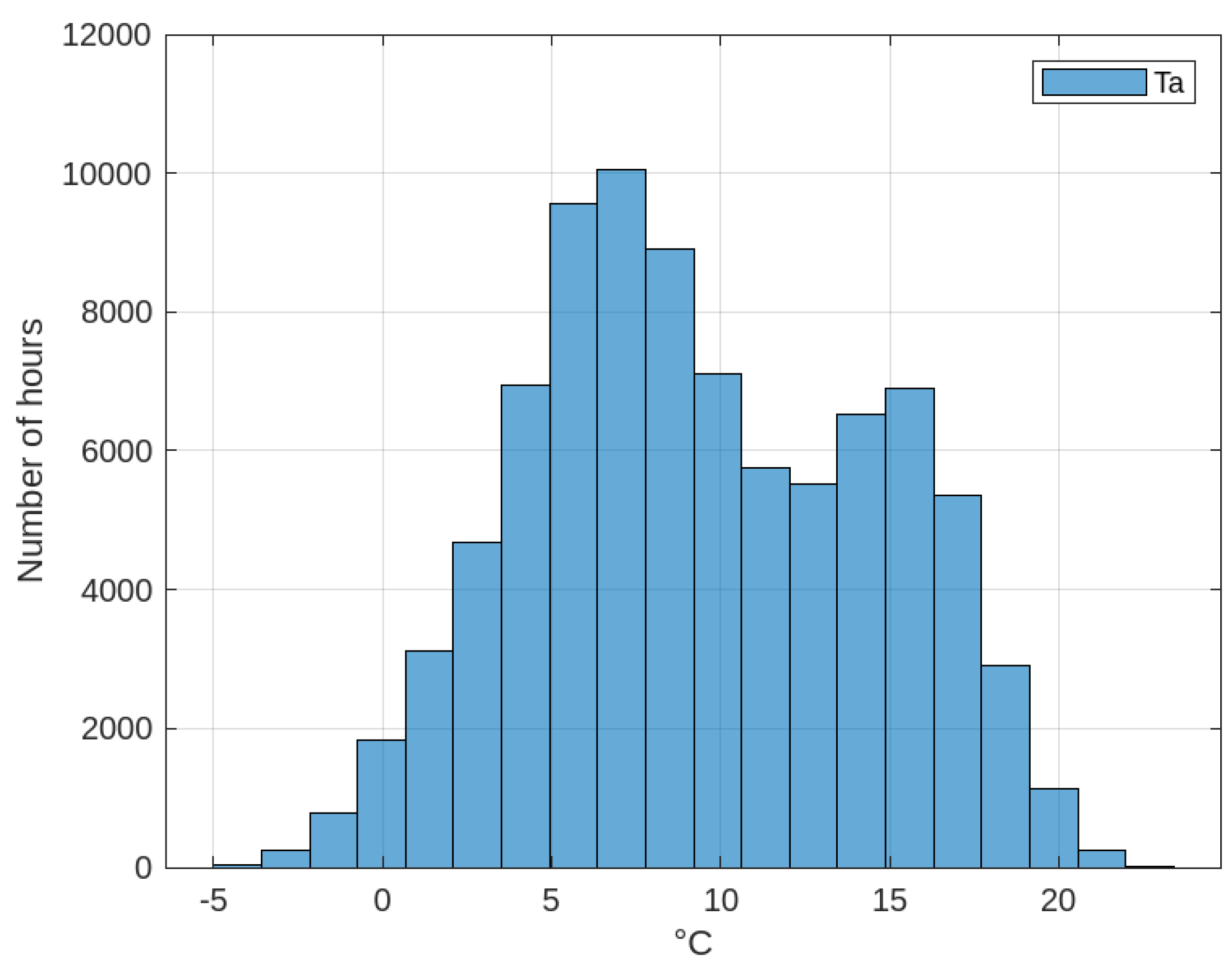
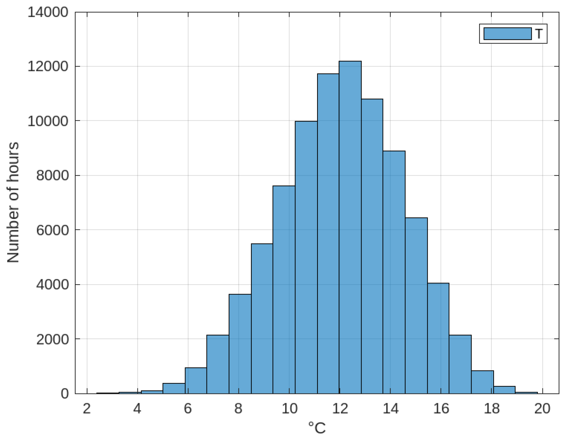
In Case Study No. 4 in Section 2, histograms of ambient and body temperature are shown, which must be analyzed. Using the MATLAB Curve Fitter Toolbox [13], the distribution function associated with the ambient and body temperature data, which is normal, can be determined. The mathematical expression of the normal distribution function is shown in Equation (107), where $\lambda$ is the standard deviation and $\mu$ is the mean. However, MATLAB’s Curve Fitter Toolbox [13] defines it according to Equation (108), where $a_1$ and $c_1$ are coefficients and $b_1$ is the mean; therefore, $b_1=\mu$. 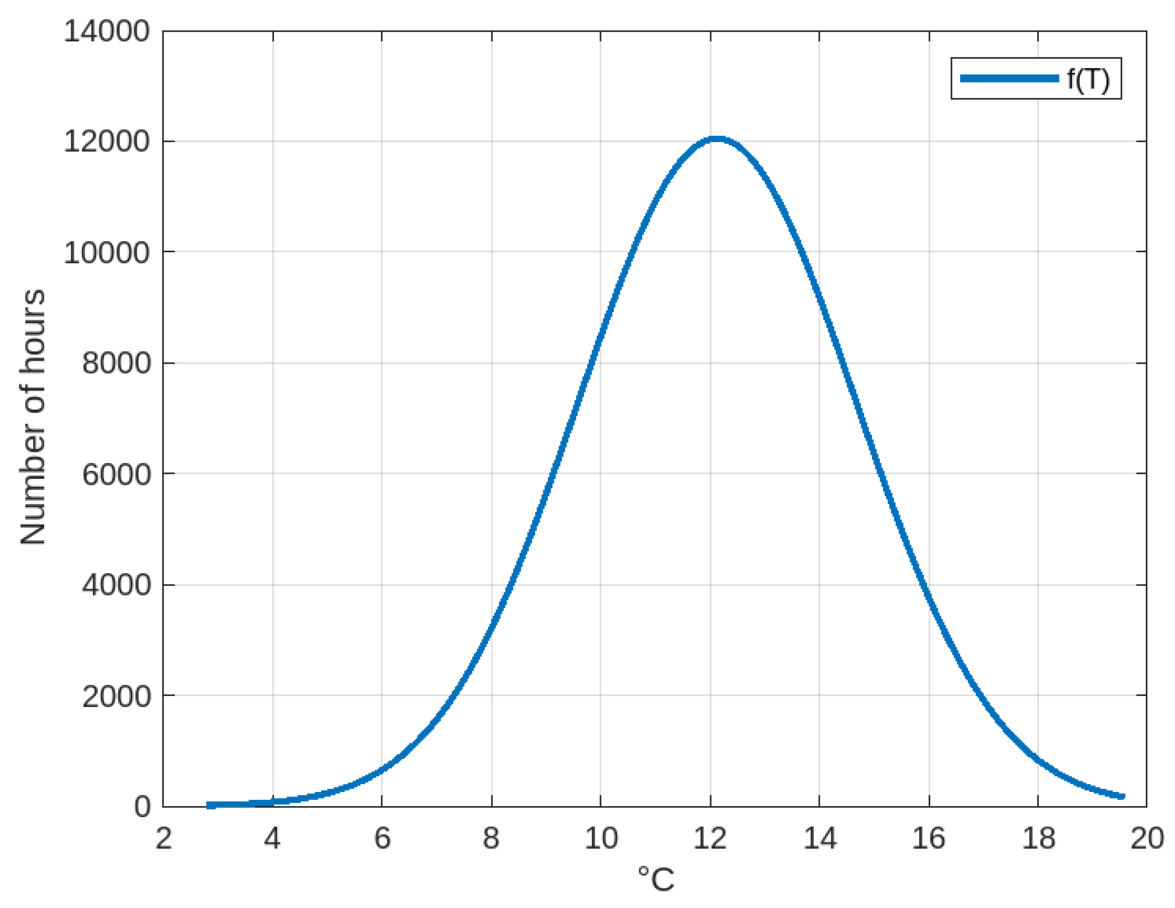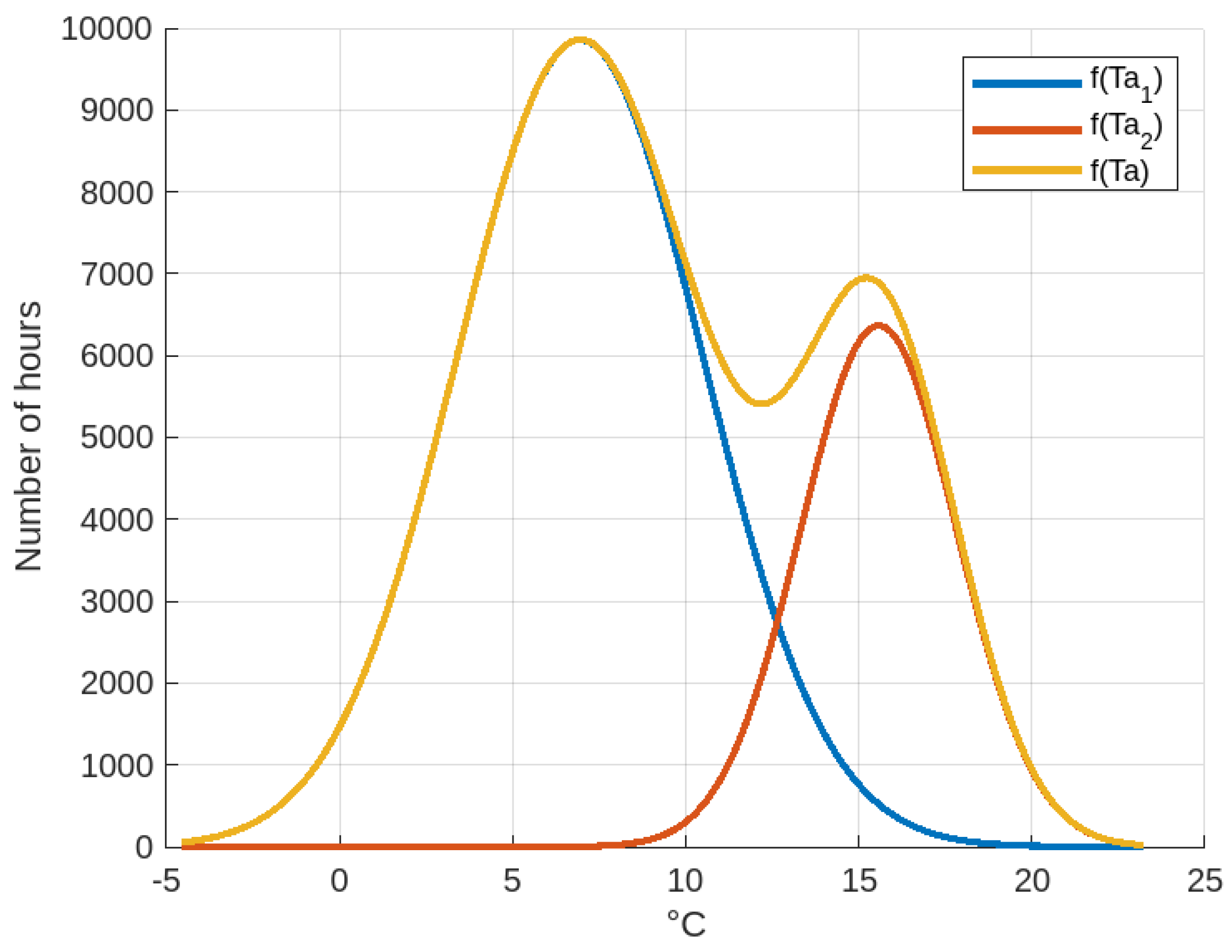Thus, the normal distribution function of body temperature shown in Figure 22 is obtained, whose mathematical expression is Equation (109) with coefficients $a_1=1.2047\times {10}^4$, $b_1={\mu }_T=12.1280$, where ${\mu }_T$ is the mean value of the normal distribution function of body temperature, $c_1=3.5925$, and the R-square is 0.9983. In the case of ambient temperature, the distribution function $f\left(Ta\right)$ consists of two normal distribution functions shown in Figure 23 as $f\left(T{a}_1\right)$ and $f\left(T{a}_2\right)$, whose mathematical expression is Equation (110) and whose coefficients are $a_2=9.857\times {10}^3$. $b_1={\mu }_{T{a}_1}=6.9464$, where ${\mu }_{T{a}_1}$ is the mean value of the normal distribution function $f\left(T{a}_1\right)$ of body temperature, $c_1=5.033$, $a_2=6.3677\times {10}^3$, $b_2={\mu }_{T{a}_2}=15.5732$, where ${\mu }_{T{a}_2}$ is the mean value of the normal distribution function $f\left(T{a}_2\right)$ of body temperature, $c_2=3.1969$, and the R-square = 0.9968. The two mean values (${\mu }_{T{a}_1}=6.9464$ $°$C,${\mu }_{T{a}_2}=15.5732$) $°$C of the normal distributions that make up the ambient temperature distribution would represent the two climatic seasons that occur during the year (summer, winter) and during each day (a marked difference between daytime and nighttime temperatures), which are characteristic of the climate at that altitude above sea level (approx. 3880 m.a.s.l.). However, the mean body temperature value ${\mu }_T=12.1280$ $°$C is unique and forms part of a normal distribution function, unaffected by daily, seasonal, and annual climate variations, and demonstrates the buffering effect of the WWT thermal energy storage system.

$$f\left(x\right)={\displaystyle \frac{1}{\lambda \sqrt{2\pi }}}{e}^{-{\displaystyle \frac{{(x-\mu )}^2}{2{\lambda }^2}}}$$

(107)

$$f\left(x\right)=a_1{e}^{-{\left[{\displaystyle \frac{(x-b_1)}{c_1}}\right]}^2}$$

(108)

$$f\left(T\right)=a_1{e}^{-{\left[{\displaystyle \frac{(T-b_1)}{c_1}}\right]}^2}$$

(109)

$$f\left(T_a\right)=f\left(T{a}_1\right)+f\left(T{a}_2\right)=a_2{e}^{-{\left[{\displaystyle \frac{(T{a}_1-b_2)}{c_2}}\right]}^2}+a_3{e}^{-{\left[{\displaystyle \frac{(T{a}_2-b_3)}{c_3}}\right]}^2}$$

(110)

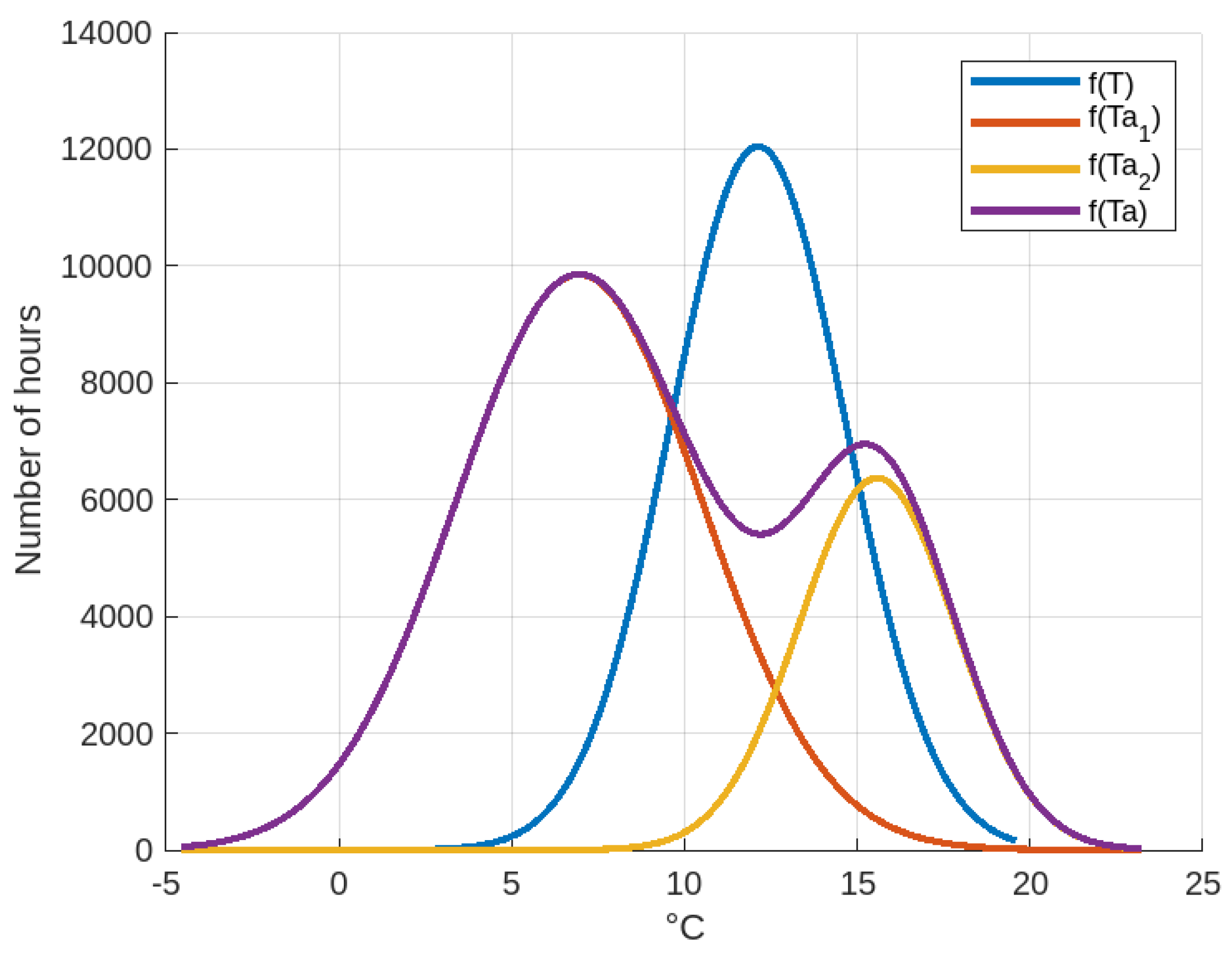
Of interest are the standard deviation values $\lambda$ of the distribution functions, which are determined by the mathematical relationship $c_1^2=2{\lambda }^2$, which leads to $\lambda =c_1/\sqrt{2}$, obtained by equating Equations (107) and (108). Then, (a) the standard deviation of the normal distribution function of body temperature ${\lambda }_T$ is ${\lambda }_T=3.5925/1.4142=2.5403$ $°$C, and (b) the standard deviations of the normal distribution functions ${\lambda }_{T{a}_1}$ and ${\lambda }_{T{a}_2}$, which make up the distribution function of the ambient temperature, are ${\lambda }_{T{a}_1}=5.033/1.4142=3.5589$ $°$C and ${\lambda }_{T{a}_2}=3.1969/1.4142=2.2605$ $°$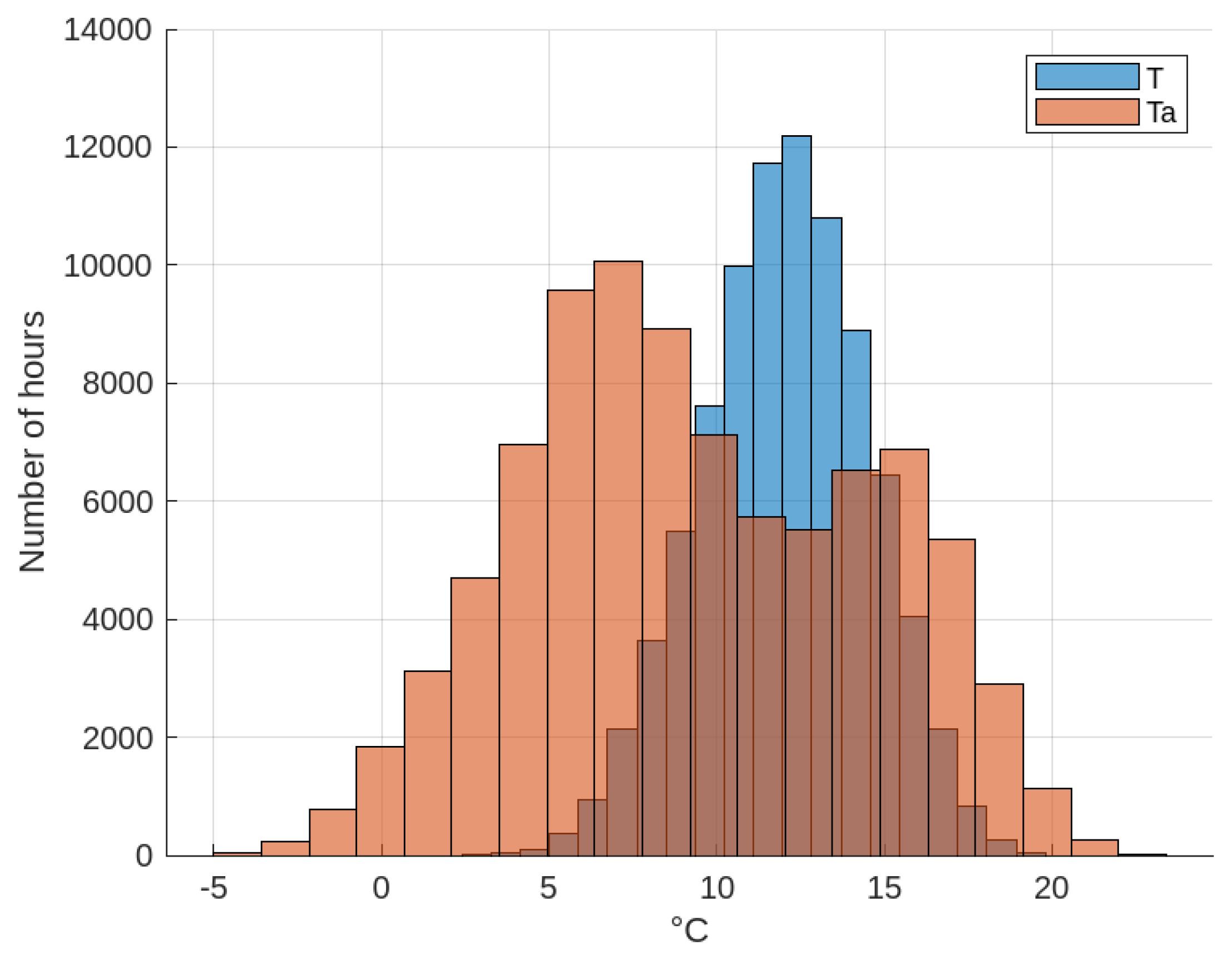C, respectively. A superposition of the normal distribution functions of body and ambient temperature is shown in Figure 24. So, if the mean value of body temperature ${\mu }_T=12.1280$ $°$C, this means that (a) 68.2% of the values of the normal distribution of body temperature lie between the values from ${\mu }_T-{\lambda }_T=9.5877$ $°$C to ${\mu }_T+{\lambda }_T=14.6683$ $°$C, and (b) 95.4% of the values in the normal distribution of body temperature are between the values from ${\mu }_T-2{\lambda }_T=7.0474$ $°$C to ${\mu }_T+2{\lambda }_T=17.2086$ $°$C, which suggests that the body (water) has allowed the storage of thermal energy (capture and delivery) in such a way that the body temperature (and therefore, the temperature of the crop fields) is maintained at values that are permissible for crops, with no freezing of water or rapid changes in body temperature.

Analyzing the model and results obtained during the development of this research, given the dimensions of the WW components, the boundary conditions are not relevant to the overall thermal behavior of the thermal energy storage system. However, this does not mean that it is not an interesting topic that should be investigated in future work or by other researchers. The maximum time interval considered in this paper was 10 years, with a large amount of hourly data that supported the conclusion that the WWT is a thermal energy storage system. Furthermore, the methodology used by NASA for the environmental temperature and solar radiation data has been detailed. However, one recommendation is to perform an analysis with paleo-archaeological environmental temperature and solar radiation records and/or simulations of the thermal behavior of the WWT in other places that archaeological evidence describes as having been built and used.

The mathematical model developed in this paper led to calculations which were made or can be made based on sums and multiplications (both possible utilizing a calculation tool called yupana) and data taken from experiments. In addition, while conducting experiments, measuring parameters with instruments as presented in other papers is not required; instruments or some techniques for measuring temperature, solar radiation and time are necessary. The results could be transmitted to farmers through quipus or similar, as if they were a technical construction standard, or transmitted verbally to instruct them on how they should build.

Most probably—given that the Inca Empire was well-organized—technical experts were the ones who taught, trained, and supervised the construction and operation of the WW, a technique that demonstrates the maximum use of energy resources available on-site sustainably, both in terms of capture and storage, for the cultivation of agricultural products. This knowledge was preserved and continued to be passed down from generation to generation, and the fields continued to be used and preserved for generations, leading to the physical archaeological evidence that exists today.

Regarding its practical applicability, recent use has been reported (at least until the last century, it was used extensively). However, I believe there are two things to consider in order for it to be reconsidered as a practice in agriculture: (a) research should be conducted on updating and/or adjusting dimensions due to climate changes that may have occurred over the last 3000 years; (b) field tests should be conducted on soil performance (nutrients, nitrogen, etc.) for certain crops commonly grown in the study area, for example, quinoa, given that it is possible that the crop fields, due to abandonment and/or ignorance of the advantages of the WWT, have lost their nutrients and need to be replenished through natural processes (small animal excrement, etc.) or artificial processes (artificial fertilizers, etc.).

Regarding extensions of the study, future research could investigate the thermal behavior of a WWT in which the soil platforms are semicircular and sets of linear soil platforms are arranged radially, surrounded in both cases by water channels. This would be a good complement to what is reported in this paper, which considered soil platforms that are linear and arranged in parallel. A more general case would be mathematical modeling, numerical simulation, and/or experimental data collection from a large-area crop field, where WWs are organized in different ways (parallel, perpendicular, semicircular, radial, etc.). I believe that despite the apparent randomness, everything was adequately studied, calculated, planned, and used as large thermal energy storage systems.

6. Conclusions

The mathematical model and the geometric shapes studied here allow us to describe, explain, and understand the Inca and pre-Inca technique used for thermal energy storage in crop fields—and in use for more than 2000 years—called Waru-Waru (WW). In essence, the most appropriate geometric shapes have been defined and studied—according to principles of fluid mechanics, thermodynamics, and heat transfer—for the best preservation of temperature for agricultural purposes. In addition, this paper provides a theoretical framework that can be used to carry out the experimental part in the laboratory and/or crop fields. The theoretical and experimental framework has been elaborated in accordance with its calculation and information storage instruments: yupana and quipu. From this, it has been proposed and argued that Incas (and pre-Incas) dominated higher mathematics, mainly that based on addition and multiplication, such as linear programming. They did not use complex mathematical expressions, which can be explained given that the objective was the common benefit of the population and that the constructions can last a long time and/or have been implemented. And globally, the technique and the populations in charge of each cultivation zone developed sustainable thermal energy storage systems (STESSs), which allowed the cultivation of agricultural production from ancestral generations to the recent and/or current ones that are still using it in the Peruvian Altiplano.

Future work includes conducting detailed studies on the problem of boundary conditions with the construction of a scale model (or a full-scale model in crop fields) of WW, for which a certain number of sensors must be placed along the boundary and used to record data on water temperature, soil platform temperature, and ambient temperature, solar radiation, and other necessary parameters (possibly soil moisture, soil electrical conductivity, etc.) using a SCADA system or similar. These measurements should be taken every second (desirable) or every minute to identify sudden changes and new phenomena (processes) in the WWT. All of this can be considered part of a future validation plan.

Another recommendation is to review the chronicles (or similar documents) and archaeological evidence to deduce and/or explain their high mathematics. The research subsequent to what is presented in this document may be to study more complex geometries and consider convection, radiation, and thermal conduction, but to maintain the consideration that they used the calculations, information storage techniques, and instruments of that time. If the experimental part is to be carried out now, it has to consider the climatic variations that have occurred during the last few decades and centuries due to global warming. Other variables to consider are the loss of the habit of cultivating land (abandoned WW) and the reduction in the amount of water in Lake Titicaca (decrease in the height of the lake’s water body), among others.

References

1. de Lozada, D.S.; Baveye, P.; Riha, S. Heat and moisture dynamics in raised field systems of the lake Titicaca region (Bolivia). Agric. For. Meteorol. 1998, 92, 251–265. [Google Scholar] [CrossRef]
2. Lhomme, J.; Vacher, J. Modelling nocturnal heat dynamics and frost mitigation in Andean raised field systems. Agric. For. Meteorol. 2002, 112, 179–193. [Google Scholar] [CrossRef]
3. Smith, C.T.; Denevan, W.M.; Hamilton, P. Ancient Ridged Fields in the Region of Lake Titicaca. Geogr. J. 1968, 134, 353. [Google Scholar] [CrossRef]
4. Bandy, M.S. Energetic efficiency and political expediency in Titicaca Basin raised field agriculture. J. Anthropol. Archaeol. 2005, 24, 271–296. [Google Scholar] [CrossRef]
5. Rashid, F.L.; Al-Obaidi, M.A.; Alsebeei, M.M.; Alkhekany, Z.A.; Ameen, A.; Ahmad, S.; Chibani, A.; Kezzar, M.; Agyekum, E.B.; Alshammari, A. Enhancing solar greenhouse efficiency through the integration of phase change materials: Thermal regulation and sustainable crop growth. Energy Build. 2025, 337, 115667. [Google Scholar] [CrossRef]
6. Lorenzo, P.; Reyes, R.; Medrano, E.; Granados, R.; Bonachela, S.; Hernández, J.; López, J.C.; Magán, J.J.; del Amor, F.M.; Sánchez-Guerrero, M.C. Hybrid passive cooling and heating system for Mediterranean greenhouses. Microclimate and sweet pepper crop response. Agric. Water Manag. 2024, 301, 108937. [Google Scholar] [CrossRef]
7. Rucins, A.; Viesturs, D.; Narvils, M.; Ivanovs, S.; Auce, A. Use of accumulated solar thermal energy in greenhourse for extending vegetation period of crop plants. Eng. Rural. Dev. 2023, 628–635. [Google Scholar] [CrossRef]
8. Ajarostaghi, S.S.M.; Amiri, L.; Poncet, S. Application of Thermal Batteries in Greenhouses. Appl. Sci. 2024, 14, 8640. [Google Scholar] [CrossRef]
9. Agho, C.; Avni, A.; Bacu, A.; Bakery, A.; Balazadeh, S.; Baloch, F.S.; Bazakos, C.; Čereković, N.; Chaturvedi, P.; Chauhan, H.; et al. Integrative approaches to enhance reproductive resilience of crops for climate-proof agriculture. Plant Stress 2025, 15, 100704. [Google Scholar] [CrossRef]
10. Stackhouse, P. POWER|DAV. Available online: https://power.larc.nasa.gov/data-access-viewer/ (accessed on 11 May 2025).
11. Stackhouse, P. POWER|Data Sources. Available online: https://power.larc.nasa.gov/docs/methodology/data/sources/ (accessed on 11 May 2025).
12. Catepillán, X.; Szymanski, W. Counting and arithmetic of the INCa. DOAJ Dir. Open Access J. 2012, 5, 47–62. Available online: https://doaj.org/article/b50844ae6af642bbb81b38e831cb65b0 (accessed on 11 May 2025).
13. MathWorks Inc. MATLAB. Available online: https://matlab.mathworks.com/ (accessed on 11 May 2025).
Figure 1. Schematic representation of the “Waru-Waru” technique (WWT) implemented in field crops.
Energies 18 03116 g001
Figure 2. Heat flow on square-section body.
Energies 18 03116 g002
Figure 3. Heat flow on square-section body and convection process.
Energies 18 03116 g003
Figure 4. Concept of discretization of the function f ( t ) in time by means of subfixes i.
Energies 18 03116 g004
Figure 5. Heat flow on circular-section body.
Energies 18 03116 g005
Figure 6. Solar irradiance evolution used as one of the input data for testing the evolution of body temperature behavior (with ϕ f = 2 ).
Energies 18 03116 g006
Figure 7. Evolution of body temperature and ambient temperature during test days (09). Initial body temperature: 7.02 °C (with ϕ f = 2 ).
Energies 18 03116 g007
Figure 8. Evolution of body temperature and ambient temperature with different ϕ f values. Test days: 09. Initial body temperature: 7.02 °C.
Energies 18 03116 g008
Figure 9. Evolution of body temperature and ambient temperature over 9 days from 23 February to 2 March 2024, with latitude −15.38 and longitude −69.95, according to data obtained from [10]. Initial body temperature: 7.02 °C.
Energies 18 03116 g009
Figure 10. Hourly ambient temperature (air) evolution over a 10-year study period (1 January 2010–31 December 2019).
Energies 18 03116 g010
Figure 11. Body temperature evolution per hour over a study period of 10 years (1 January 2010–31 December 2019).
Energies 18 03116 g011
Figure 12. Histogram of hourly ambient temperature at a location with coordinates of latitude −15.38 and longitude −69.95, and an observation period of 10 years (1 January 2010–31 December 2019).
Energies 18 03116 g012
Figure 13. Histogram of hourly body temperature at a location with coordinates of latitude −15.38 and longitude −69.95, and an observation period of 10 years (1 January 2010–31 December 2019).
Energies 18 03116 g013
Figure 14. Histograms of hourly body and ambient temperatures at coordinates of latitude −15.38 and longitude −69.95; observation period: 10 years (1 January 2010–31 December 2019).
Energies 18 03116 g014
Figure 15. Experimental–theoretical process of WW design.
Energies 18 03116 g015
Figure 16. Scheme of thermal flow and temperatures on square-section body and convection process.
Energies 18 03116 g016
Figure 17. Geometric representation of two bodies showing the flow of thermal energy without convection.
Energies 18 03116 g017
Figure 18. Scheme of thermal flow and temperatures between two bodies without convection.
Energies 18 03116 g018
Figure 19. Geometric representation of two bodies showing the flow of thermal energy considering conduction and convection with air.
Energies 18 03116 g019
Figure 20. Geometric representation of three bodies showing the flow of thermal energy considering conduction and convection with air.
Energies 18 03116 g020
Figure 21. Geometric representation of many bodies showing the flow of thermal energy considering conduction between bodies and bodies–soil, and convection between bodies and air.
Energies 18 03116 g021
Figure 22. Normal distribution function of body temperature obtained using MATLAB’s Curve Fitter Toolbox [13].
Energies 18 03116 g022
Figure 23. Normal distribution function of ambient temperature obtained using MATLAB’s Curve Fitter Toolbox [13].
Energies 18 03116 g023
Figure 24. Normal distribution functions of body temperature and ambient temperature (and their component distribution functions) obtained using MATLAB’s Curve Fitter Toolbox [13].
Energies 18 03116 g024
Disclaimer/Publisher’s Note: The statements, opinions and data contained in all publications are solely those of the individual author(s) and contributor(s) and not of MDPI and/or the editor(s). MDPI and/or the editor(s) disclaim responsibility for any injury to people or property resulting from any ideas, methods, instructions or products referred to in the content.