Article

Research on Day-Ahead Optimal Scheduling of Wind–PV–Thermal–Pumped Storage Based on the Improved Multi-Objective Jellyfish Search Algorithm

1
School of Electrical and Electronic Engineering, Hubei University of Technology, Wuhan 430068, China
2
Hubei Engineering Research Center for Safety Monitoring of New Energy and Power Grid Equipment, Hubei University of Technology, Wuhan 430068, China
*
Author to whom correspondence should be addressed.
Energies 2025, 18(9), 2308; https://doi.org/10.3390/en18092308
Submission received: 16 April 2025 / Revised: 27 April 2025 / Accepted: 29 April 2025 / Published: 30 April 2025
(This article belongs to the Section B: Energy and Environment)

Abstract

:
As the share of renewable energy in modern power systems continues to grow, its inherent uncertainty and variability pose severe challenges to grid stability and the accuracy of traditional thermal power dispatch. To address this issue, this study fully exploits the fast response and flexible operation of variable-speed pumped storage (VS-PS) by developing a day-ahead scheduling model for a wind–photovoltaic–thermal–VS-PS system. The optimization model aims to minimize system operating costs, carbon emissions, and thermal power output fluctuations, while maximizing the regulation flexibility of the VS-PS plant. It is assessed using the improved multi-objective jellyfish search (IMOJS) algorithm, and its effectiveness is demonstrated through comparison with a fixed-speed pumped storage (FS-PS) system. Simulation results show that the proposed model significantly outperforms the traditional FS-PS system: it increases renewable energy accommodation capacity by an average of 68.51%, reduces total operating costs by 14.13%, and lowers carbon emissions by 3.63%.

1. Introduction

In the global effort to tackle climate change and promote sustainable development, achieving peak carbon and carbon neutrality has become a core national goal. In this context, building a new type of power system is viewed as an important pathway to achieve the “dual carbon” target. The development of this system relies on technological innovation and system optimization. It aims to become greener, lower in carbon emissions, smarter, and more flexible. The extensive use of renewable energy such as wind and PV is a key feature of this energy transition. These sources not only significantly reduce fossil fuel consumption and carbon emissions, but also drive the optimization and upgrading of the energy structure [1]. However, the large-scale grid integration of wind and PV energy brings issues of intermittency and fluctuation. This may lead to imbalances in power supply and demand. Traditional approaches often use thermal power units for peak regulation to cope with wind and PV output fluctuations. With the continuous growth of wind and PV capacity, traditional thermal power faces challenges such as low regulation efficiency and poor economic performance [2]. These challenges make it difficult to meet grid stability requirements. Research shows that large-scale energy storage is the key to solving this problem. Therefore, combining pumped hydro storage with wind–PV–thermal integrated energy systems has become a research focus. Traditional FS-PS units always operate at a fixed-rated power. This limits their ability to adapt flexibly to load changes [3]. As a result, their regulation capability and response speed are restricted. To address this challenge, VS-PS technology has emerged [4,5]. Compared to fixed-speed units, VS-PS offers stronger regulation ability and adaptability. It can respond more efficiently to random wind and PV output fluctuations. This improves the overall stability and operating efficiency of the system. Therefore, using VS-PS to mitigate the impact of large-scale wind and PV integration has become an inevitable trend in modern power system development [6].
The authors of [7] built a microgrid power generation system integrating PV power, wind power, and VS-PS. The study optimized its dispatch strategy to improve economic benefits. It proposed an optimal hourly management model to achieve coordinated operation between wind and PV power and VS-PS. The authors of [8] proposed a joint dispatch model based on seawater-pumped storage. The study innovatively realized energy storage and seawater desalination with the same equipment. This approach reduced capital investment and operating costs. In addition, it combined seasonal pumped storage with thermal energy storage. This combination enabled cross-season energy dispatch and was especially suitable for systems with highly variable renewable energy. The authors of [9,10] explored the combination of small-scale floating PV systems and VS-PS in hilly regions. The study used existing reservoirs for energy storage and the integration of renewable energy. This integration improved the renewable energy ratio and system reliability in microgrids. The authors of [11] studied an independent hybrid renewable energy system that integrated PV power, battery storage, and VS-PS. The focus was on reducing the over-sizing of system components while ensuring power supply reliability. The goal was to minimize the cost of power supply. The authors of [12] proposed an innovative integrated power generation system. This system combined off-river pumped storage with floating PV technology. The approach aimed to overcome the limitations of traditional pumped hydro storage in terms of site selection, structure, and environmental adaptability. The study also developed an optimized hybrid energy power system dispatch model. The objective was to reduce operating costs and improve overall economic benefits. The authors of [13,14] built a microgrid dispatch system that combined PV energy, wind power, and VS-PS. The study focused on ensuring sustainable energy supply, reducing energy costs, and improving energy security in remote areas. The authors of [15] proposed an optimal fuel mix dominated by zero-carbon energy. They developed an integrated energy dispatch model that included wind, PV, VS-PS, and electric vehicles. The goal was to help cities achieve decarbonized energy systems. The authors of [16] investigated the use of abandoned mining resources to build a microgrid system. This system integrated VS-PS, wind power, and PV power. The aim was to cope with extreme weather challenges and improve the stability and efficiency of the power system. The authors of [17] constructed a wind power and FS-PS system. A priority ordering method was used for optimized dispatch. The optimal dispatch results for the combined wind and pumped storage output were then used to schedule the operation of thermal power units. The authors of [18] used the energy system of Ireland as a case study. Their study focused on the role of FS-PS storage in increasing wind power accommodation, optimizing operating scale, and reducing costs. The results showed that this system improved wind power utilization and reduced operating costs. The authors of [19] addressed microgrid systems’ economic, emission, and multi-objective dispatch issues. They developed a microgrid dispatch model that combined VS-PS, pumped thermal energy storage, wind power, PV power, and battery storage. The experimental results demonstrated that the model improved dispatch efficiency and reduced computational complexity, achieving a balance between economic and environmental benefits. The authors of [20] took the northern China regional power grid as a study object. They constructed a large-scale integrated energy dispatch model that combined wind power, PV power, and VS-PS. The research focused on enhancing system stability and dispatch flexibility. However, it did not consider wind and PV power curtailment or total operating costs. The authors of [21] designed a microgrid system with rooftop PV power generation and FS-PS. The design was based on the characteristics of the buildings. In addition, a cost-benefit analysis was conducted to assess the project’s feasibility. The authors of [22] proposed a micro-scale VS-PS unit for microgrids. The system utilized building height for pumped storage and released water for power generation when needed. The study also optimized Load Frequency Control (LFC) using an artificial sheep flock algorithm. This approach addressed frequency stability issues caused by fluctuations in renewable energy. It achieved good results in multi-area control. The authors of [23] proposed a power generation system that combined wind power, hydropower, and VS-PS based on local microgrids. The research showed that the system had a high degree of self-sufficiency. In addition, pumped storage technology significantly improved the efficiency of wind power systems. The authors of [24] constructed an islanded operation system combining wind, hydropower, thermal power, and VS-PS. The results showed that the introduction of VS-PS reduced system dispatch costs by 2.5% to 11%.
Table 1 demonstrates that current research on VS-PS optimization primarily focuses on microgrid applications, while traditional FS-PS remains the mainstream solution in large-scale pumped storage studies. Notably, comparative analyses between VS-PS and FS-PS configurations in large-scale power generation systems exhibit certain deficiencies. Furthermore, in utility-scale power systems, the development of comprehensive operational frameworks that synergize wind power, photovoltaic, thermal power, and VS-PS for peak shaving and valley filling has not been adequately explored. Existing research still lacks integrated models incorporating VS-PS into large-scale integrated energy systems for multi-energy complementary coordinated dispatch, with limited comparative analysis of scheduling optimization effects between VS-PS and FS-PS in such systems. To enrich research in this field, this paper establishes a large-scale joint dispatch model encompassing wind power, photovoltaic, thermal power, and VS-PS, conducting comparative studies with FS-PS systems. The model simultaneously optimizes three critical objectives: (1) minimizing the total system operating costs, (2) reducing output fluctuations of thermal power units, and (3) decreasing carbon emissions. Through quantitative analysis and comparison of these three objectives, this study evaluates the impacts of FS-PS and VS-PS configurations on renewable energy accommodation capacity and system economic performance in large-scale integrated energy systems.

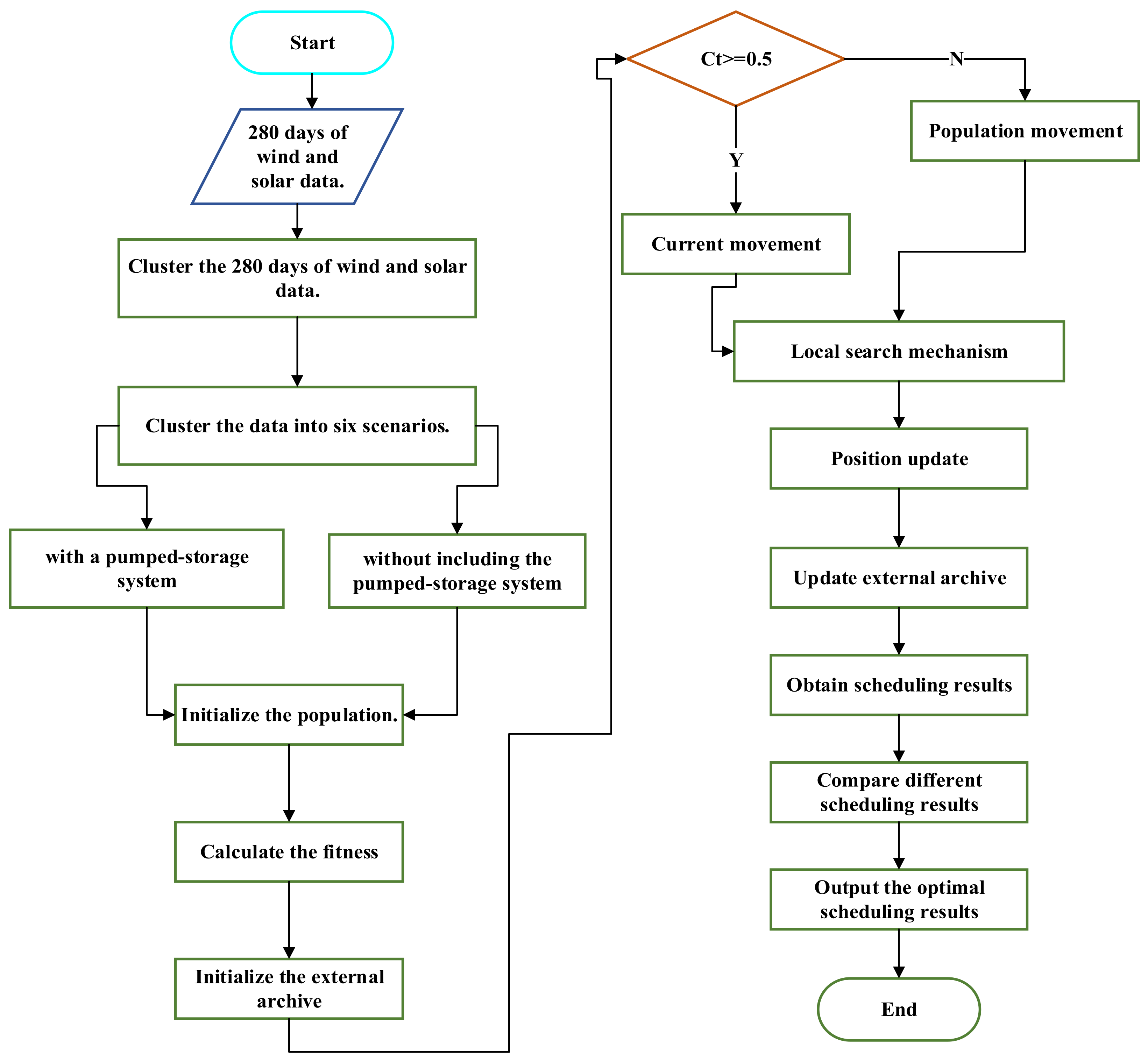
2. Typical Scenario Division

Wind and PV power generation is influenced by meteorological conditions and seasonal changes. It shows different output characteristics at different times and locations. To address this challenge, this paper proposes a data-driven scenario classification method based on generation characteristics. Using clustering algorithms, the study captures the fluctuation patterns of wind and PV power and classifies meteorological variations. This method reflects the seasonal and monthly variations of wind and PV generation. It also identifies key operational scenarios. This, in turn, improves the adaptability and generalization of scheduling strategies. In particular, this paper applies the mean shift algorithm to cluster annual data. This approach avoids the limitation of verifying effectiveness within a single scenario. By analyzing data from different dates and scenarios, the study improves day-ahead scheduling accuracy. It effectively predicts potential anomalies and system failures and enhances the robustness of scheduling strategies. Using 280 days of wind and PV output data for clustering provides a solid foundation for long-term planning and decision-making [25,26].

2.1. Mean Shift Clustering Algorithm

The mean shift algorithm is a non-parametric clustering method based on kernel density estimation. It identifies high-density regions in the data by smoothing the data distribution. The algorithm does not require predefinition of the number of clusters and can detect clusters of arbitrary shapes. It is a centroid-based algorithm. The core idea is to update candidate centroid points by averaging the points within a given region. In the post-processing stage, these points are filtered to eliminate near-duplicates. This results in a final set of centroids. The mean shift algorithm uses Kernel Density Estimation (KDE) to estimate the probability density function of data points. This study chooses the kernel function as a Gaussian kernel and expresses it as follows:
K ( x ) = exp ( x 2 2 ) ,
The mean shift vector is used to update the position of data points, moving them towards the local maximum of the density function. The calculation formula for the mean shift vector is as follows:
m ( x ) = i = 1 n x i K ( x x i h ) i = 1 n = 1 K ( x x i h ) x ,
where x i is the data point and h is the bandwidth parameter.

2.2. Clustering Scenarios

This study uses 280 days of operational data from a wind farm and a solar photovoltaic plant. We applied cluster analysis and divided the data into six scenarios: low wind–low solar, medium wind–low solar, low wind–high solar, high wind–high solar, high wind–low solar, and medium wind–high solar. To validate these clusters, we calculated the silhouette coefficient as well as the Calinski–Harabasz and Davies–Bouldin indices. These three metrics together provide a clear assessment of clustering quality.
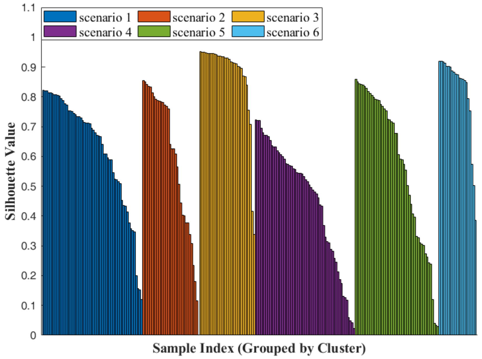
  • Clustering Validity Analysis
In order to thoroughly assess the validity of the clustering results, this study adopts three widely recognized evaluation metrics: the Mean Silhouette Coefficient, the Calinski–Harabasz Index, and the Davies–Bouldin Index. The Mean Silhouette Coefficient ranges from −1 to 1. Values approaching 1 indicate that samples are highly cohesive within their respective clusters and well-separated from neighboring clusters, reflecting an excellent clustering structure. Values near 0 suggest ambiguous cluster boundaries and moderate clustering performance, while negative values imply that certain samples may have been incorrectly assigned to inappropriate clusters. The Calinski–Harabasz Index measures the ratio of between-cluster dispersion to within-cluster compactness, with higher values indicating more distinct and compact clusters. Typically, a value greater than 500 is considered indicative of good clustering quality. The Davies–Bouldin Index assesses the average similarity between each cluster and its most similar counterpart. A lower Davies–Bouldin Index value signifies better separation and compactness, where a value below 0.5 suggests excellent clustering performance and a value between 0.5 and 1.0 indicates good clustering quality. Figure 1 presents the silhouette coefficient distribution for all samples, and Table 2 summarizes the specific values of the three evaluation metrics, offering a clear and comprehensive evaluation of the clustering effectiveness.
According to Table 2, the average silhouette coefficient of the clustering results is 0.613, significantly exceeding the commonly accepted threshold of 0.5. This suggests that the samples are highly cohesive within their respective clusters and well-separated from neighboring clusters. The Davies–Bouldin Index is 0.542, approaching the ideal value of 0.5, which further confirms that the six identified scenarios exhibit clear boundaries and strong internal compactness. Moreover, the Calinski–Harabasz Index reaches a high value of 710.7, highlighting the superior quality of the clustering in terms of maximizing inter-cluster differences and minimizing intra-cluster variance. Taken together, the favorable performance across all three evaluation metrics demonstrates that the adopted clustering approach effectively captures the distinct wind–solar output patterns with high stability and reliability, thereby laying a robust foundation for subsequent scheduling optimization and system performance assessment.
2.
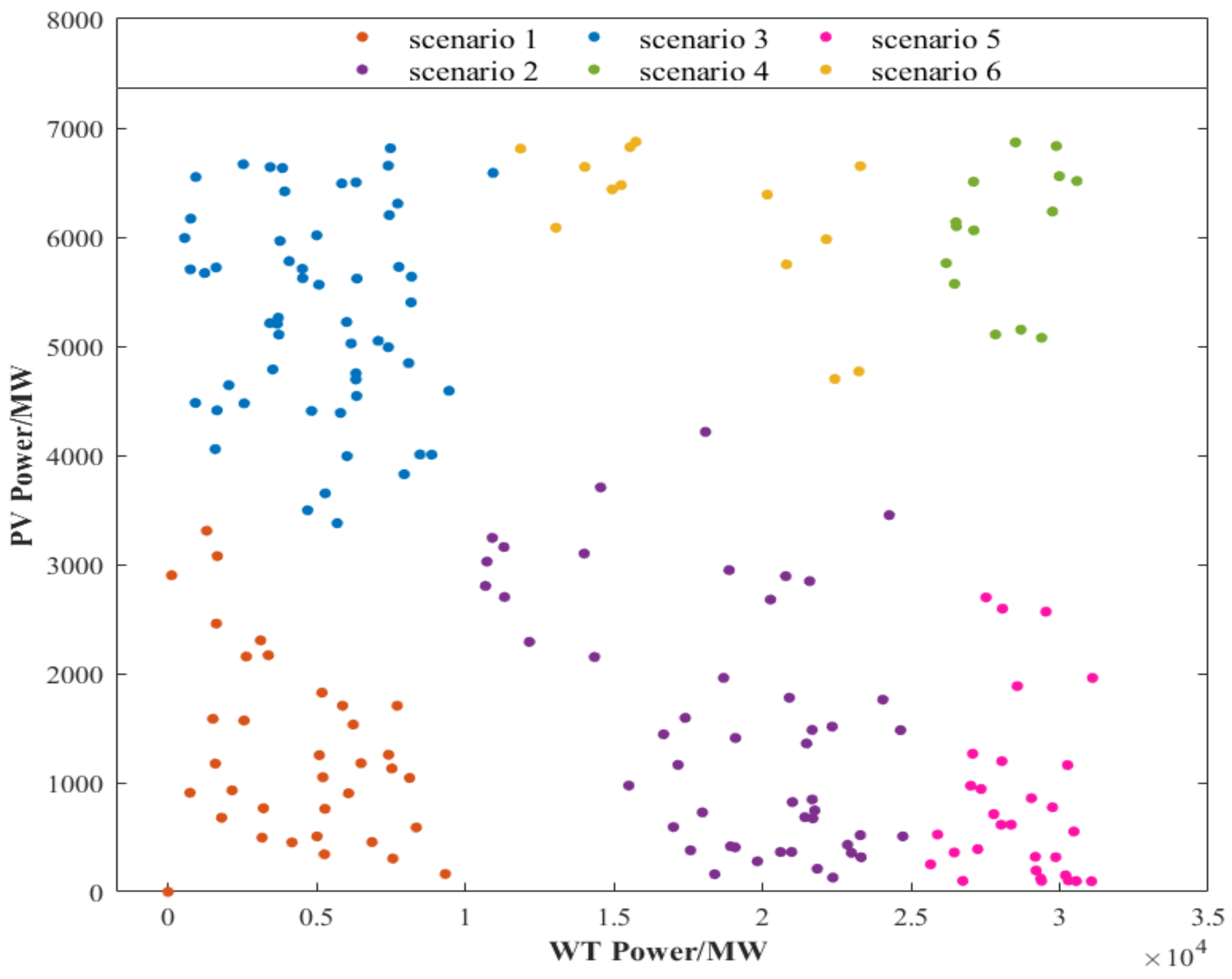
Clustering Results Presentation
The classifications identified in this study reflect the combined characteristics of wind and solar power outputs across various operating scenarios, offering important insights into the distribution patterns of renewable energy generation. These findings contribute to the optimization of dispatch strategies, the achievement of system balance, and the design of integrated energy systems. Figure 2 presents the clustering results, and Table 3 details the relationship between the defined scenarios and the clustering outcomes. Four representative clusters were selected for further analysis: Strong Wind and Strong Light, Strong Wind and Weak Light, Weak Wind and Weak Light, and Weak Wind and Strong Light. These clusters display wind and solar generation outputs along with corresponding load profiles. Compared to typical daily data, each cluster exhibits clear and representative characteristics, accurately capturing generation patterns under different wind–solar conditions and greatly enhancing the representativeness and practical applicability of the clustering results.
One day was selected from each of the six scenarios. Table 3 lists the specific dates used as the base experimental data.
The wind and PV output curves, as well as the load curves for each typical scenario, are shown in Figure 3.
Figure 3 shows that PV output primarily occurs during daylight hours. The general trend of PV generation remains consistent across different seasons and broadly aligns with the load variation, contributing positively to peak shaving. In contrast, wind power generation exhibits significant randomness, with large daily fluctuations. Wind output is higher in the early morning and evening, showing characteristics of valley filling. Additionally, weather conditions and seasonal variations highly influence wind power generation, exhibiting notable differences across different periods.

3. Improved Multi-Objective Jellyfish Search Algorithm

3.1. Multi-Objective Jellyfish Algorithm

MOJS is an emerging population-based optimization algorithm inspired by the foraging and group behavior of jellyfish in nature. Chou and Truong proposed MOJS in 2021 as an extension of the single-objective Jellyfish Search Algorithm (JSA). The JSA efficiently searches by simulating the jellyfish’s strategies of following ocean currents, group cooperation, and random swimming. There are three main mechanisms of jellyfish foraging behavior: current tracking (moving toward the global optimum), intra-group movement (attraction or repulsion between individuals to balance exploration and exploitation), and dynamic time control (adjusting the concentration or dispersion of the search strategy). With its few parameters, fast convergence, and strong global search ability, the JSA has quickly become an effective tool for solving complex optimization problems [27,28].
MOJS generally has two types of movement patterns for jellyfish individuals: ocean current movement and population-based individual movement. When Ct1 > 0.5, the movement of jellyfish is considered under the influence of ocean currents; when Ct1 < 0.5, the movement of jellyfish individuals in the population is considered; these two movement patterns simulate the jellyfish’s behavior of hunting and exploring the environment in the ocean. The core purpose of each movement pattern is to allow the jellyfish individuals to effectively explore the solution space and find the global optimum. The control functions are as follows:
C t 1 = ( 1 t / T ) ( 2 r a n d ( 0 , 1 ) 1 )
In the formula, Ct1 represents the original dynamic adjustment parameter; t is the current iteration number; T is the maximum number of iterations.
Limitations of the Algorithm:
MOJS shows potential in global exploration and diversity maintenance. However, its limited local search capability and design flaws in key parameters, such as the time control parameter Ct, significantly constrain the algorithm’s performance.
(1)
Weak local search capability: The core mechanism of the JSA is centered around random drifting and current-following strategies. This results in limited capability for fine-tuning when approaching the Pareto front. In complex, multi-modal solution spaces, the algorithm faces difficulties in enhancing the convergence precision of the solution set through effective neighborhood search, often leading to a dispersed distribution of solutions or divergence from the true Pareto front.
(2)
The original Ct1 parameter employs a linear decay mechanism, leading to a lack of adaptability in transitioning between global exploration and local exploitation: the linear variation of (1 − t/T) causes the algorithm’s exploration capability to rapidly diminish in the early stages, potentially resulting in premature convergence to local optima. The uniform distribution of the random component (2*rand−1) leads to a fixed perturbation amplitude, preventing dynamic adjustment of the search step size according to the iteration stage. This rigidity hampers the algorithm’s ability to adapt to the evolving demands of complex multi-objective problems, resulting in insufficient global search time and persistent ineffective perturbations in later stages, thereby reducing optimization efficiency.
(3)
Insufficient diversity maintenance mechanism: The algorithm lacks an adaptive neighborhood design tailored to the multi-objective characteristics. For example, it does not dynamically adjust the search step size based on the correlation between objectives, which further reduces the effectiveness of the local search.
To address these issues, the authors of [29] proposed adding an elite retention strategy to the multi-objective jellyfish algorithm. This prevents high-quality solutions from being lost during iterations. It improves both convergence speed and accuracy. The authors of [30] proposed a method that uses segmented chaotic mapping (SPM) to generate the initial positions of the jellyfish population. This method takes advantage of the ergodicity and randomness of chaotic systems. It makes the initial population more uniformly distributed in the search space, avoiding clustering issues seen in traditional random initialization and enhancing the algorithm’s global search ability. The authors of [31] proposed a dynamic weight-based initialization scheme for low-carbon flexible job-shop scheduling. In this scheme, 30% of the population is generated randomly to ensure diversity, while the remaining 70% is selected dynamically to improve workshop efficiency. The authors of [32] addressed the problem of the original jellyfish algorithm falling into local optima by introducing a Lévy flight strategy. The algorithm can occasionally jump out of local regions by using long-distance random steps. This expands the search range and reduces the risk of premature convergence. The authors of [33] introduced significant improvements to the Musical Chairs Algorithm (MCA), including gradually eliminating the worst solutions to enhance computational efficiency, incorporating Lévy flights to balance global and local search, optimizing the stopping criteria to improve convergence stability, and extending it to a binary version Musical Chairs Algorithm (BMCA) for feature selection. These enhancements significantly accelerate convergence, reduce the risk of getting trapped in local optima, and ensure the algorithm’s stability, making it exceptionally effective in optimization tasks. The authors of [34] proposed a Nested Particle Swarm Optimization (NESTPSO). NESTPSO employs two nested PSO loops to automatically optimize control parameters and swarm size. The inner loop minimizes the objective function, while the outer loop uses premature convergence rate and iteration count as fitness metrics. This design effectively balances exploration and exploitation, significantly enhancing convergence speed and reliability. Although the advancements in single-objective optimization methods, such as those in the MCA and NESTPSO, cannot be directly employed as comparative algorithms in this work, they provide valuable insights that have significantly inspired the improvements made in our study.
This paper improves motion control parameters to expand the search range and find better solutions. It introduces a mechanism that generates neighborhood solutions for more precise searching to enhance local search.

3.2. Algorithm Improvement

3.2.1. Improvement of Time Control Parameter

This study proposes an improved decay mechanism by introducing a power exponent. In MOJS, the motion control parameter Ct1 undergoes dynamic nonlinear decay adjustments: early stage (t is small): setting p close to 0.5 slows down the decay, maintaining high perturbations to enhance global exploration. Later Stage (t is large): Setting p close to 1.5 accelerates the decay, reducing random disturbances to focus on local exploitation. The random component is dynamically scaled by (1 − t/T)p, allowing for large perturbations early on to boost diversity and smaller perturbations later to improve convergence stability. In the early phase of the algorithm, automatically adjusting the exponent p helps balance exploration and exploitation by applying large random perturbations that maintain population diversity and enhance global search. Experiments show that when p is near 0.5, the decay is slowest and the perturbation magnitude is largest, so we set the initial p to 0.5. Preliminary tests with p = 0.3, 0.5, and 0.7 confirmed that p = 0.5 delivers the most robust convergence across benchmark functions and applications. In future work, one could run small-scale pilot studies over [0.3, 1.0], tailored to problem complexity and dimensionality, to assess how different initial p values impact convergence speed and solution quality and then choose the optimal starting exponent.
C t 2 = ( 1 t / T ) p ( 2 r a n d ( 0 , 1 ) 1 )
p = 0.5 + t T
In the formula, Ct2 represents the improved dynamic adjustment parameter; p is the dynamic adjustment factor.

3.2.2. Local Search Mechanism

The local search algorithm optimizes the solution by performing “small-step probing” near the current solution. Specifically, the algorithm generates multiple “neighboring solutions” near the current solution through random perturbations, which can be seen as exploring a region around the solution in the search space. The perturbation’s step size determines the search range’s width: a larger step size allows the algorithm to move beyond the current local region, avoiding local optima. A smaller step size enables finer adjustments to improve solution precision. A newly generated solution will automatically return to the boundary if it exceeds the predefined feasible domain. Then, the algorithm decides whether to replace the current solution by comparing multiple objectives, where the new solution is at least as good as the current one in all objectives and better in at least one. Through this repeated process of exploration and comparison, the local search not only explores the search space within the framework of global search but also delves deeper into potential key regions, ultimately leading to a solution set closer to the ideal and more evenly distributed.
Δ j = S ( t ) ( U [ 0 , 1 ] n 0.5 )
S ( t ) = S o   ·   ( 1 t T ) 0.5
In this equation, Δ j represents the j-th random perturbation vector, where each component follows a uniform distribution U[−0.005, 0.005]; S(t) is the step size; and the initial step size of S o is 0.005.
X j , i n e i g h b o r = X c u r r + Δ j
In this equation, X j , i n e i g h b o r represents the neighborhood position, and X c u r r represents the current position.
X j , i b o u n d e d = var min , i ( i f   X j , i n e i g h b o r < var min , i ) var max , i ( i f   X j , i n e i g h b o r > var max , i ) X j , i n e i g h b o r ( o t h e r w i s e )
In this equation, X j , i b o u n d e d represents the feasible solution after boundary handling, var min , i represents the lower boundary after boundary handling, and var max , i represents the upper boundary after boundary handling.
X n e w = N o n   D o m i n a t e d   B e s t ( { X j , i b o u n d e d , X c u r r } )
In this equation, X n e w represents the output position, and N o n   D o m i n a t e d   B e s t is performed to select the optimal position.
The flowchart of the improved IMOJS algorithm is shown in Figure 4:

3.2.3. Weight Assignment and Optimal Solution Selection

In this study, the Entropy Weight Method is employed to objectively assign weights to the three objectives, followed by the application of the Technique for Order of Preference by Similarity to Ideal Solution (TOPSIS) technique to identify the optimal solution from the Pareto front.
(1)
Weight determination based on the Entropy Method
In the first step, the Pareto solution set is formulated as the initial decision matrix.
In the second step, the entropy values are computed based on Equations (11) and (12).
M i j = x i j i = 1 n x i j
i = 1 n M i j = 1
In these equations, M i j represents the proportion matrix; x i j is the original objective value at the i-th row and j-th column; and n denotes the number of solutions in the Pareto solution set.
In the third step, the entropy value is calculated according to Equation (13).
e j = 1 ln n i = 1 n M i j ln M i j
In this equation, e j represents the entropy value calculated for the three objectives.
The fourth step is to calculate the divergence coefficient for the three objectives based on their entropy values.
d j = 1 e j
In this equation, d j represents the divergence coefficient calculated for the three objectives.
The fifth step is to normalize and obtain the weights using Equations (15) and (16).
w j = d j k = 1 3 d k
j w j = 1
In these equations, w j represents the weight of the j-th objective.
(2)
Optimal Solution Selection in TOPSIS
The weights required for selecting the Pareto solution set using TOPSIS have been calculated, and then TOPSIS is applied to select the Pareto optimal solution.
In the first step is to normalize the original solution set using Equation (17).
r i j = x i j i = 1 n x i j 2
In this equation, r i j represents the normalized matrix.
The second step is to construct the weighted normalized matrix using the weights calculated above.
v i j = w j · r i j
In this equation, v i j represents the weighted normalized matrix.
The third step is to identify the positive ideal solution and the negative ideal solution.
v j + = ( min v i 1 , min v i 2 , min v i 3 )
v j = ( max v i 1 , max v i 2 , max v i 3 )
In these equations, v j + represents the positive ideal solution; v j represents the negative ideal solution.
The fourth step is to calculate the Euclidean distance.
D i + = j = 1 3 ( v i j v j + )
D i = j = 1 3 ( v i j v j )
In these equations, D i + represents the distance between the i-th solution and the positive ideal solution; D i represents the distance between the i-th solution and the negative ideal solution.
The fifth step is to calculate the proximity.
C i = D i D i + + D i
In this equation, C i represents the proximity of the i-th solution.
The sixth step is to rank the solutions in the Pareto solution set based on their proximity, and select the solution with the highest proximity as the optimal solution.

3.3. Simulation Experiments

In the algorithm comparison experiments, we retained the original Multi-Objective Jellyfish Search (MOJS) algorithm as our baseline for improvement and selected three classic multi-objective optimization algorithms as benchmarks: Multi-Objective Evolutionary Algorithm based on Decomposition (MOEA/D), Strength Pareto Evolutionary Algorithm 2 (SPEA2), and Nondominated Sorting Genetic Algorithm III (NSGA-III). Over the past five years, this combination has been used as the control group in 83% of highly cited energy-related studies (Elsevier Scopus) and 92% of algorithm improvement papers published in IEEE Transactions on Evolutionary Computation (TEVC). These algorithms are widely recognized as the “gold standard” in evolutionary computation and have been extensively validated in top-tier journals such as IEEE TEVC, with detailed records of their performance characteristics and limitations. Specifically, the decomposition strategy of MOEA/D has proven highly effective in handling complex constraints, making it widely applicable to energy system optimization tasks such as microgrid scheduling and unit commitment. SPEA2, with its fast convergence in low-dimensional spaces, has become the tool of choice for tuning industrial control parameters. NSGA-III’s reference point mechanism effectively mitigates the curse of dimensionality in high-dimensional objective problems. Using these algorithms as benchmarks helps ensure the interpretability and reproducibility of the comparative results across different fields. Our experiments were conducted on the PlatEMO platform. In all experiments, the population size for each algorithm was set to 200, and each algorithm was executed independently 30 times. Finally, we presented the maximum, average, and minimum values for each performance metric, with the first row representing the maximum values, the second row the average values, and the third row the minimum values.
The experimental setup uses the classic DTLZ series test functions as the benchmark platform. This test set includes optimization problems with various objective dimensions (three to eight) and complex characteristics. Each test function provides a known reference Pareto front, which allows for a comprehensive evaluation of algorithm convergence and distribution in high-dimensional spaces. The performance of NSGA-III, MOJS, and IMOJS is assessed using three classical metrics: Hypervolume (HV): Measures the coverage area of the solution set. A larger HV value indicates better diversity and distribution. Generational Distance (GD): Measures the distance between the solution set and the true Pareto front. A smaller GD value signifies that the solution set is closer to the true Pareto front. Inverted Generational Distance (IGD): Evaluates the distribution and coverage of the solution set. A smaller IGD value indicates that the solution set is closer to the actual Pareto front. The bold font in the table represents the optimal value among the five algorithms in the experiment. To highlight the key findings, this section presents only a portion of the comparative data and the main conclusions (the complete dataset is provided in Appendix A).
Table 4 compares the three algorithms based on the HV metric.
According to the experimental results in Table 4, MOEA/D achieved higher maximum HV values under three objectives than IMOJS on the DTLZ2 test function. At the same time, SPEA2 surpassed IMOJS on DTLZ3, and NSGA-III demonstrated superior minimum HV values compared to IMOJS. In five-objective scenarios, NSGA-III obtained higher maximum HV values than IMOJS on DTLZ1, whereas MOEA/D outperformed IMOJS on both DTLZ3 and DTLZ6. For eight objectives, MOEA/D achieved higher maximum HV values than IMOJS on DTLZ3, while MOJS exhibited better average HV values than IMOJS on DTLZ4. Although these HV values were higher than IMOJS’s, the differences remained within the percentile range. Additionally, IMOJS demonstrated superior HV values in 77.8% of cases within the DTLZ benchmark test set compared to MOJS, NSGA-III, MOEA/D, and SPEA2.
Table 5 shows the comparison data of the three algorithms in terms of the GD metric.
Based on the experimental results presented in Table 5, for the DTLZ2 test function with three objectives, the MOEA/D algorithm outperforms IMOJS in terms of the GD minimum value; with eight objectives, the NSGA-III algorithm performs better in terms of the GD minimum value. Regarding the DTLZ4 test function, the NSGA-III algorithm surpasses IMOJS in the GD minimum value for five objectives and the GD average value for eight. In the DTLZ5 test function with three objectives, the NSGA-III, MOEA/D, and SPEA2 algorithms all outperform IMOJS regarding the GD minimum value. For the DTLZ6 test function, the MOJS algorithm exceeds IMOJS in both the maximum and average values for three objectives; the NSGA-III algorithm shows better GD values for the minimum value with five objectives; and for the GD maximum value with eight objectives, the NSGA-III algorithm also outperforms IMOJS, though the difference remains within the percentile range. Additionally, IMOJS achieves 79.63% of GD values superior to MOJS, NSGA-III, MOEA/D, and SPEA2 in the DTLZ benchmark test set.
Table 6 presents the comparison data for the three algorithms regarding the IGD metric.
The experimental results in Table 6 reveal the following performance analyses for the DTLZ2, DTLZ5, and DTLZ6 test functions: For DTLZ2, NSGA-III outperforms IMOJS in IGD maximum value with three and five objectives and achieves a lower IGD minimum value with eight objectives. In DTLZ5, SPEA2 shows a better IGD minimum value with three objectives, while NSGA-III outperforms IMOJS in IGD minimum value with eight objectives. For DTLZ6, MOEA/D provides a better IGD minimum value with five objectives, and NSGA-III surpasses IMOJS in IGD maximum value with eight objectives, although the difference is minimal. Additionally, IMOJS shows superior GD values to MOJS, NSGA-III, MOEA/D, and SPEA2 in 85.18% of cases across the DTLZ benchmark test set.
Based on the experimental data from Table 4, Table 5 and Table 6, IMOJS shows significant performance advantages on the DTLZ test set. Compared to NSGA-III, MOJS, MOEA/D, and SPEA2, the algorithm has a numerical advantage in three key evaluation metrics: HV, GD, and IGD. This advantage confirms its excellent multi-objective optimization capability. Regarding HV, the core metric reflecting the convergence and distribution of the solution set, the data in Table 3 show that IMOJS achieves better hypervolume values in over 77.8% of the test cases. This result indicates that the algorithm can accurately approximate the Pareto front and highlights its unique mechanism for maintaining population diversity. Further analysis of the GD and IGD metrics (Table 5 and Table 6) shows that IMOJS outperforms other algorithms with smaller distance measures in more than 79.6% of the test cases. The superior performance in the GD metric validates the algorithm’s breakthrough in solution convergence accuracy. In contrast, the comprehensive advantage in the IGD metric indicates that the solution sets generated by IMOJS are geometrically closer to the actual Pareto front. This dual advantage emphasizes the effective balance between exploration and exploitation in IMOJS.
Through systematic validation across the three metrics, IMOJS performs better on the DTLZ test set. It shows an average of 80.8% higher values in key metrics such as HV, GD, and IGD compared to the other four algorithms, confirming its outstanding effectiveness in multi-objective optimization problems.

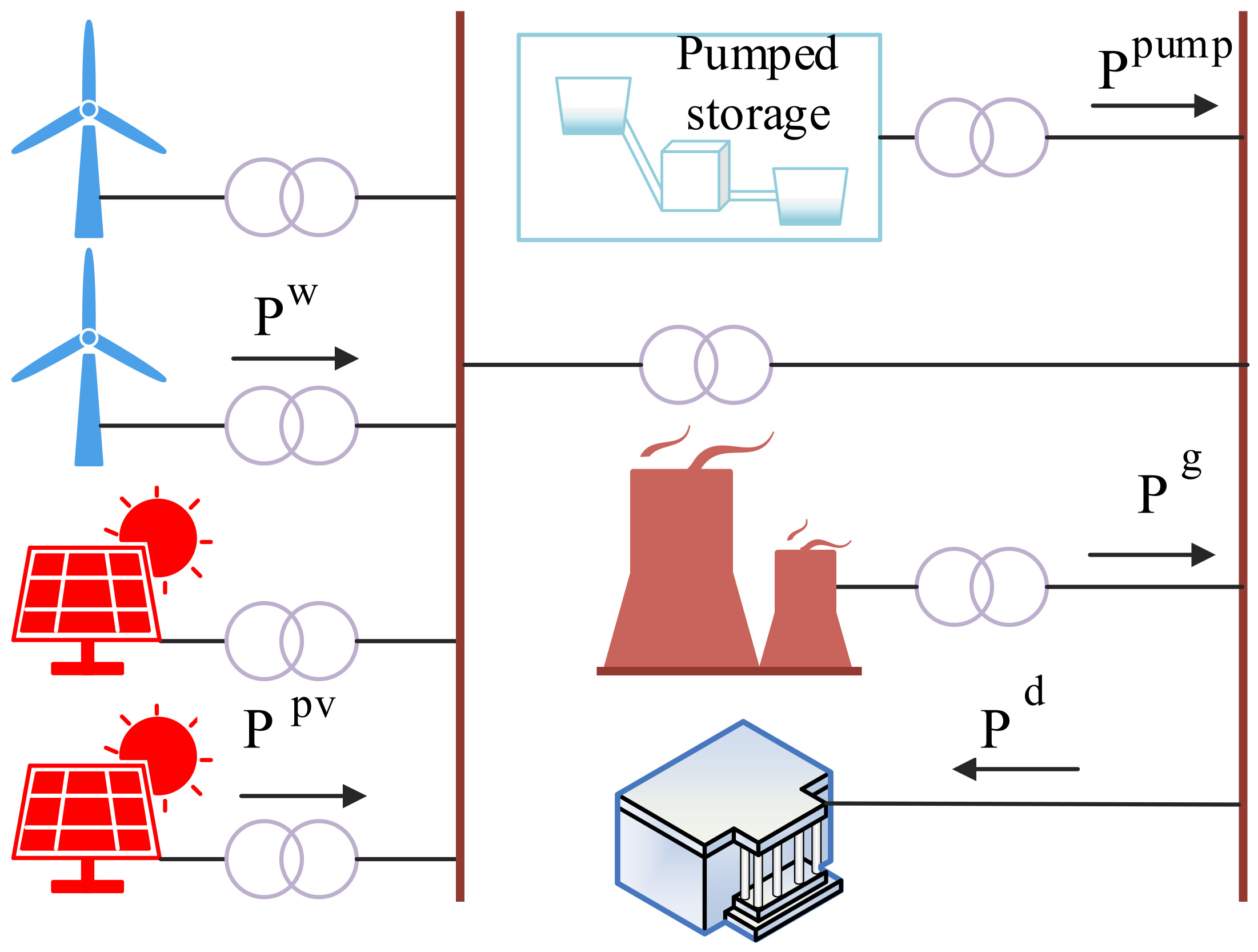
4. Wind–PV–Thermal–Pumped Storage System Model

Due to the intermittency and variability of wind and PV power, relying solely on these two energy sources makes it difficult to ensure the stable operation of the power system. In this context, constructing an efficient integrated energy system becomes particularly important. Thermal power plants have strong peak-shaving capabilities and can provide a stable power supply when wind and PV generation are insufficient. Pumped storage power stations effectively store surplus wind and PV power, releasing it during peak demand to balance supply and demand, enhancing system stability and operational efficiency. This system, through the integration and mutual regulation of multiple energy forms, strengthens the stability and reliability of the power system, promoting the optimization of the energy structure and clean, low-carbon development. With the rapid development of pumped storage technology, current research has shifted from traditional fixed-speed pumped storage FS-PS to VS-PS. Compared to fixed-speed units, variable-speed pumped storage offers significant advantages such as flexible power regulation, quick response to load fluctuations, and continuous bidirectional power adjustment, which can more efficiently smooth out renewable energy output fluctuations and improve system regulation capacity [35]. This paper constructs a multi-objective optimization model for the wind–PV–thermal–storage joint operation system with variable-speed pumped storage to minimize carbon emissions, optimize joint operation costs, and minimize thermal power unit output fluctuations. To assess the practical benefits of variable-speed pumped storage, the paper uses an IMOJS to solve the wind–PV–thermal–storage joint operation system. It sets up a dual-scenario experiment, including variable-speed and fixed-speed pumped storage. The structure of the integrated energy system is shown in Figure 5.

4.1. Objective Function

Traditional integrated scheduling models often use a single economic dispatch model. This paper constructs a wind–PV–thermal–pumped storage joint optimization dispatch model with economic efficiency, environmental protection, and high-performance objectives. Considering the system’s power balance constraints and the operational constraints of wind, PV, hydro, and thermal generators, the objective function is to minimize the system’s operational cost, carbon emissions, and thermal power fluctuations.
Objective function 1.
The system considers the economic aspect of the optimization scheduling model to minimize the operating cost. The objective function for minimizing the system’s operating cost is as follows:
F 1 = t = 1 T ( z t 1 + z t 2 + z t 3 + z t 4 )
In the formula: F 1 —Total system operating costs, t —operation period, T —total operating time; z t 1 , z t 2 , z t 3 —coal-fired power generation cost, pollution control cost, and penalties for curtailed wind and PV power in time period t .
Objective function 2.
Considering environmental factors, the objective is to minimize adverse impacts and carbon emissions. The objective function focuses solely on reducing emissions from thermal power, excluding CO2 emissions from wind, PV, and pumped storage:
F 2 = ζ C O 2 × t = 1 T p i t g
In the formula: F 2 —carbon emissions; ζ C O 2 —carbon emissions per unit of electricity generation. p i t g —The output power of thermal power unit i in time period t .
Objective function 3.
Thermal power fluctuations undermine the stability of the power system, challenge the fuel supply of thermal power plants, and weaken thermal power plants’ peaking capacity. Considering system stability, the objective is to minimize thermal power fluctuations:
F 3 = i = 1 n Net i
Net i = 1 n × t = 1 T p i t g μ i 2
μ i = t = 1 T p i t g T
In the formula: F 3 —total thermal power fluctuation coefficient; Net i —fluctuation coefficient of thermal power unit i ; n —total number of thermal power units; μ i —average power output of thermal power unit i .

4.2. Operating Cost

4.2.1. Coal Cost of Thermal Power Units

The operating cost of a thermal power unit is a convex nonlinear quadratic function:
z t 1 = i = 1 Ng w [ a i ( p i t g ) 2 + b i p i t g + c i ]
In the formula: Ng —total number of thermal power units. a i , b i , c i —coal consumption coefficient of unit i ; p i t g —output power of thermal power unit i during time period t . w —coal price.

4.2.2. Pollutant Treatment Costs

The primary pollutants that thermal power plants produce are typically Nitrogen Oxides (NOx), Sulfur Oxides (SOx), and particulate matter. The total cost of treating these pollutants can be calculated as follows [36]:
z t 2 = t = 1 T i = 1 N g ( Q NO x , i +   Q SO 2 , i +   Q TSP , i )
Q NO x , i = q 1 × μ 1 × [ a i × ( p i t g ) 2 b i × p i t g + c i ]
Q SO 2 , i = q 2 × μ 2 × [ a i × ( p i t g ) 2 b i × p i t g + c i ]
Q TSP , i = q 3 × μ 3 × [ a i × ( p i t g ) 2 b i × p i t g + c i ]
In the formula: Q NO x , i , Q SO 2 , i , Q TSP , i —the treatment costs for Nitrogen Oxides (NOx), Sulfur Oxides (SOx), and particulate matter (PM) for each unit; q 1 , q 2 , q 3 —unit treatment cost; μ 1 , μ 2 , μ 3 —unit treatment coefficient. The specific experimental parameters are shown in Table 7.

4.2.3. Penalty Cost for Curtailing Wind and PV Power

The cost of curtailing wind and PV power is the sum of both:
z t 3 = t = 1 T ξ w ( ( 1 λ w ) · p t , f w p t w ) + t = 1 T ξ p v ( ( 1 λ p v ) · p t , f p v p t p v )
In the formula: ξ w —unit penalty coefficient for curtailed wind power; ξ p v —unit penalty coefficient for curtailed PV power; λ w —is the energy loss parameter of wind power generation; λ p v —is the energy loss parameter of photovoltaic power generation; p t , f w —the predicted electricity generation of the wind farm at time period t ; p t , f p v —the forecasted electricity generation of the PV power plant in time period t ; p t w —the wind power generation in the scheduling plan for time period t ; p t p v —the PV power generation in the scheduling plan for time period t .

4.2.4. Construction Cost

To ensure the cost estimation is more realistic, the construction cost is evenly distributed over each day of the system’s lifecycle, thereby making the calculation of the overall operational cost more accurate and reflective of actual conditions.
z t 4 = z t o t a l / T l i f e × 365
In the formula: z t 4 —construction cost averaged per day; z t o t a l —for the system’s total construction cost; T l i f e —for the system’s design life.

4.3. Constraints

4.3.1. System Power Balance Constraint

i = 1 Ng p i t g + p t w + p t p v + p t p u m p = p t D
In the formula: p t p u m p —the planned generation of the pumped storage power station at time t (when p t p h > 0, it indicates that the power station is in the generating state; when p t p h < 0, it indicates that the power station is in the charging state); p t D —the load value at time t .

4.3.2. Constraints of Thermal Power Units

(1)
Output Constraints of Thermal Power Units [39]
p min i g p i t g p max i g
In the formula: p min i g —the lower output limit of the i thermal power generation unit; p max i g —the upper output limit of the i thermal power generation unit.
p i t d o w n Δ t p i t g p i ( t 1 ) g p i t u p Δ t
In the formula: p i t d o w n —the derating rate limit of thermal power unit i at time t ; p i t u p —the loading rate limit of thermal power unit i at time t .

4.3.3. Pumped Storage Station Constraints [40,41]

(1)
Operational Constraints of the Pumped Storage Station
p t p u m p = δ g , t p u m p p g , t p u m p + δ p , t p u m p p p , t p u m p
0 δ g , t p u m p + δ p , t p u m p 1
W t p u m p = W t 1 p u m p ( 1 η c ) + C w Δ T η p p u m p p p , t p u m p
C w Δ Tp g , t p u m p / η g p u m p
W min p u m p W t p u m p W max p u m p
W t = 0 p u m p = W t = T p u m p
R d o w n c h · Δ t < p t + 1 c h p t c h < R u p c h · Δ t
R d o w n d i s · Δ t < p t + 1 d i s p t d i s < R u p d i s · Δ t
In the formula, δ g , t p u m p and δ p , t p u m p are Boolean variables, representing the power generation condition and the pumping condition of the pumped storage unit, respectively. p g , t p u m p , p p , t p u m p are the power generation and pumping power of the pumped storage unit at time period t, respectively. W t p u m p , W min p u m p , W max p u m p represent the upper reservoir capacity, the minimum limit, and the maximum limit of the pumped storage station at time period t, respectively. η p p u m p , η g p u m p , η c represent the efficiency of power generation, the efficiency of pumping, and the water loss rate, respectively. p t c h —pumping power at time t; R d o w n c h —maximum downward ramp rate in pumping mode; R u p c h —maximum upward ramp rate in pumping mode; p t d i s —generating power at time t; R d o w n d i s —maximum downward ramp rate in generating mode; R u p d i s —maximum upward ramp rate in generating mode. C w , Δ T , T are respectively the average water/electricity conversion coefficient, the time interval for the optimization of the pumped storage unit, and the total number of time periods within the operating cycle.
(2)
Spinning Reserve Constraint
i = 1 Ng S i g + S p u m p ( 1 + δ ) P max D
p max D = max ( p 1 D , ... , p T D )
In the formula: S i g —the installed capacity of i the thermal power unit; S p u m p —the installed capacity of the pumped storage power station; δ —the spinning reserve capacity of the system; p max D —the maximum load of the system.

4.3.4. Wind Power Constraints

Wind power scheduled dispatch power Wind power forecasted power
0 p t w p t , f w

4.3.5. PV Power Constraints

PV power scheduled dispatch power PV power forecasted power
0 p t p v p t , f p v

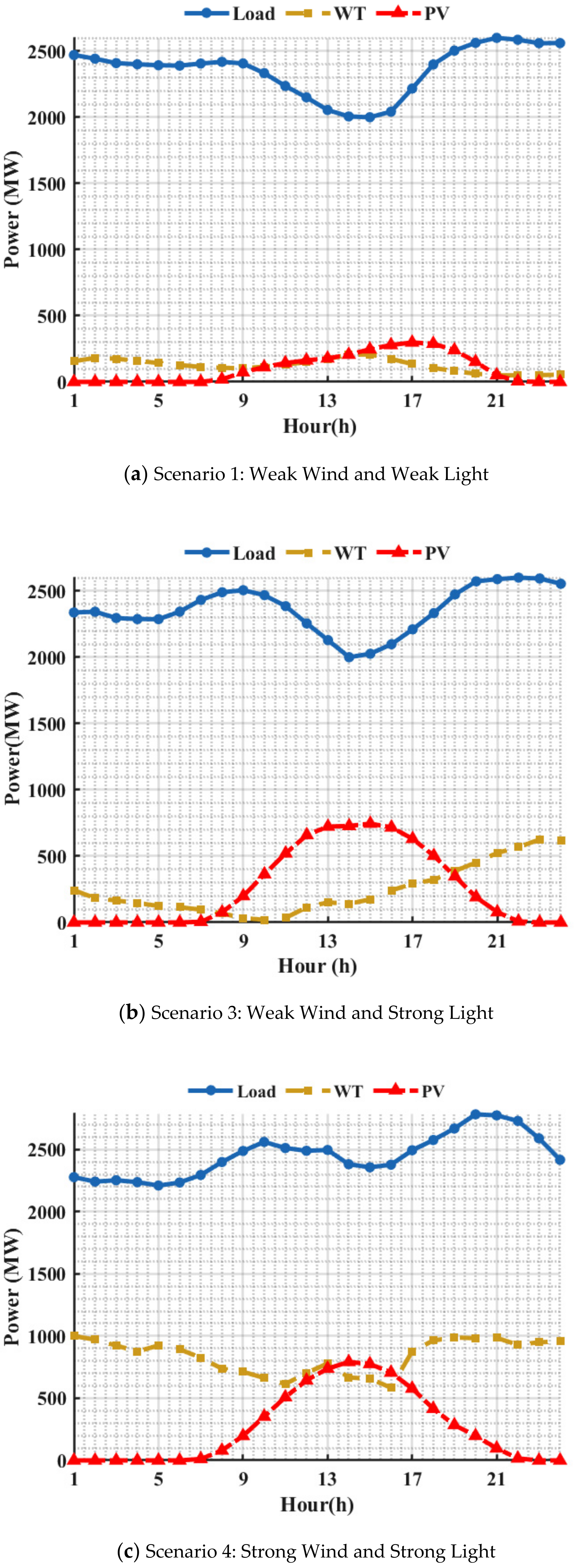
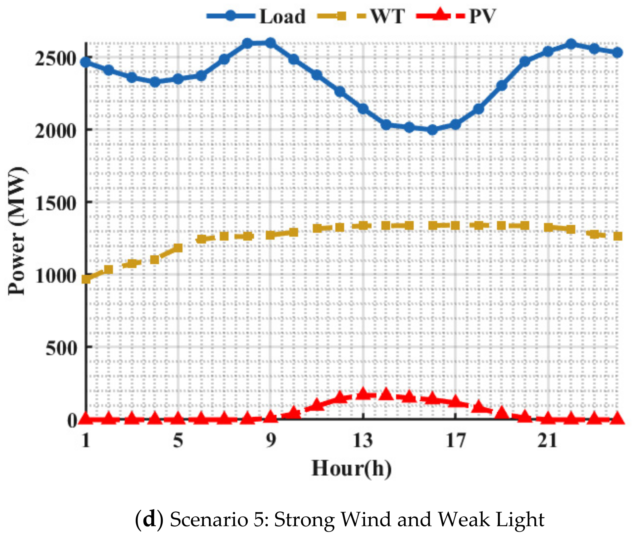
5. Simulation Results and Analysis

Figure 6 illustrates the solution process for the wind–PV–thermal–storage model and the practical application of IMOJS in the model.
Table 8 provides the installed capacities of wind, PV, and other power sources, along with some technical parameters of thermal power and pumped storage plants.

5.1. Algorithm Solving Comparison for the Real Model

In Section 3.3, simulation experiments were conducted using test functions DTLZ1 to DTLZ6, and four algorithms, including IMOJS, MOJS, and NSGA-III, were compared. The results indicate that IMOJS shows significant advantages in terms of HV, GD, and IGD. However, real-world problems are usually more complex and involve additional constraints. To further validate the capability of IMOJS in handling complex practical models, this section employs five algorithms—IMOJS, MOJS, NSGA-III, MOEA/D, and SPEA2—to solve a VS-PS model. The three objective function values obtained are then compared and analyzed. The number of iterations for each algorithm is set to 500 generations, with a population size of 500.
As shown in Table 9, IMOJS demonstrates significant advantages over other algorithms regarding system cost, CO2 emissions, and thermal power fluctuations. Specifically, IMOJS achieves the lowest system cost across all six scenarios, averaging 7.8% lower than MOJS, 3.2% lower than NSGA-III, and 12.4% lower than SPEA2. In terms of CO2 emissions, IMOJS consistently records the lowest values in all scenarios, with average reductions of 3.1% compared to MOJS, 1.3% compared to NSGA-III, and 3.8% compared to SPEA-2. Regarding thermal power fluctuations, IMOJS exhibits the smallest fluctuations in five out of six scenarios, averaging 18.7% lower than MOJS and 23.4% lower than NSGA-III. These superior performances are attributed to integrating nonlinear motion control parameters and local search strategies. The nonlinear motion control parameters introduce dynamic adjustment mechanisms, enabling the algorithm to adaptively modify search steps at different stages. This balance between global exploration and local exploitation helps prevent the algorithm from becoming trapped in local optima. Local search strategies focus on the neighborhood of the current solution, thoroughly exploring potential high-quality solutions within the solution space. This enhances the algorithm’s precision and convergence speed. Combining these two mechanisms strengthens the global search and local optimization capabilities of the algorithm, thereby improving its efficiency and effectiveness in solving complex problems.

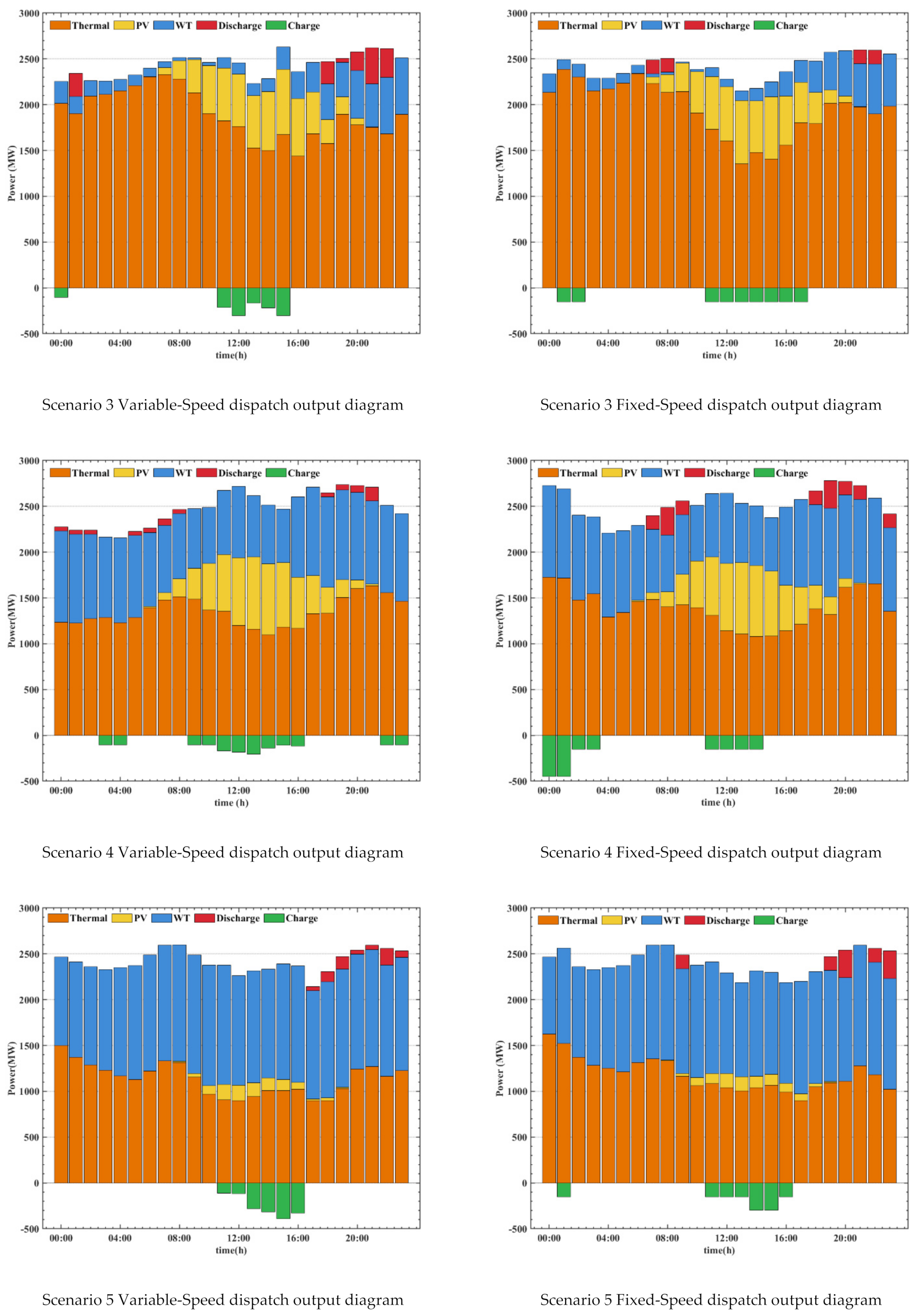
5.2. Joint Scheduling Model of Variable-Speed and Fixed-Speed Pumped Storage

This paper uses IMOJS to optimize the wind–PV–thermal–storage joint operation system to assess the practical benefits of variable-speed pumped storage. It sets up a dual-scenario experiment covering both VS-PS and FS-PS. Through an in-depth analysis of day-ahead scheduling optimization, the paper explores the application effects of different pumped storage technologies in system scheduling and their impact on power system operation. It provides data support for further improving system scheduling efficiency and economics.
As shown in Figure 7, the charging/discharging periods of VS-PS exhibit distinct patterns across different scenarios. In Scenario 1, charging primarily occurs from 00:00 to 04:00 and 11:00 to 15:00. In contrast, discharging concentrates between 16:00 and 24:00. Scenarios 3 and 5 share similar charging periods (11:00–15:00) but differ in discharging schedules: Scenario 3 discharges mainly from 19:00 to 23:00, whereas Scenario 5 maintains discharge from 15:00 to 24:00. Notably in Scenario 4, charging is concentrated in the period from 09:00 to 14:00 with discharge periods at 06:00–09:00 and 18:00–21:00, demonstrating effective mitigation of thermal power fluctuations during peak demand and absorption of renewable energy surplus during off-peak periods. FS-PS shows different operational characteristics. Scenarios 1 and 4 charge during 00:00–04:00 and 11:00–14:00 but discharge at distinct intervals: 19:00–24:00 (Scenario 1) versus 18:00–21:00 (Scenario 4). Scenarios 3–5 predominantly charge between 11:00 and 16:00, with Scenario 3 discharging briefly from 21:00 to 22:00, contrasting with Scenario 5’s extended discharge from 19:00 to 24:00. While these scheduling strategies partially alleviate thermal power fluctuations during peak periods and integrate renewable energy during valley periods, their operational flexibility appears more constrained compared to variable-speed systems.
A joint dispatch model for FS-PS and VS-PS was solved under six scenarios. The results in Table 10 include the joint operation cost, carbon emissions, and thermal power output fluctuations for both FS-PS and VS-PS in each scenario.
Based on the metrics presented in Figure 7, FS-PS exhibits relatively limited flexibility in regulation capability compared to VS-PS. Specifically, FS-PS systems demonstrate slower response times to load fluctuations and renewable energy variability, resulting in suboptimal mitigation of power grid oscillations and constrained renewable energy integration. These shortcomings highlight the inferior regulation performance and accommodation efficiency of FS-PS configurations. Based on the quantitative data from Table 10, in Scenario 1, the VS-PS model reduces joint operational costs by CNY 2.154 million, decreases carbon emissions by 1471.4 tons, and lowers thermal power output fluctuations by 132.8 units compared to the fixed-speed counterpart. Scenario 2 shows even more significant improvements, with cost savings of CNY 4.74 million, emission reductions of 1253.7 tons, and a 92.1-unit reduction in thermal output variability. Similar advantages persist across the remaining four scenarios, consistently demonstrating the variable-speed system’s superior operational efficiency and stability enhancement performance.
When comparing the operational characteristics of pumped storage units across different scenarios, VS-PS units demonstrate superior charging/discharging flexibility. These scheduling strategies partially mitigate thermal power output fluctuations during peak periods and absorb renewable generation during off-peak periods. However, FS-PS units typically operate at constant power levels with limited flexibility, potentially restricting their ability to adjust charging/discharging outputs. This inflexibility may lead to insufficient renewable energy integration, thereby compromising system stability and regulation capacity. In contrast, VS-PS units dynamically adjust their power outputs according to grid load demands and renewable generation variations. Through flexible power regulation, they effectively smooth thermal power fluctuations and enhance system stability. Simultaneously, VS-PS units demonstrate superior capability in accommodating wind and PV generation, significantly reducing curtailment rates while improving renewable energy absorption efficiency. Consequently, VS-PS outperforms FS-PS systems in regulation precision, response speed, and system support effectiveness, providing higher-quality flexible regulation resources for power systems with high renewable penetration.
This study will conduct detailed analyses from two perspectives, wind/PV curtailment levels, and operational costs, to further validate the effectiveness of variable-speed pumped storage.

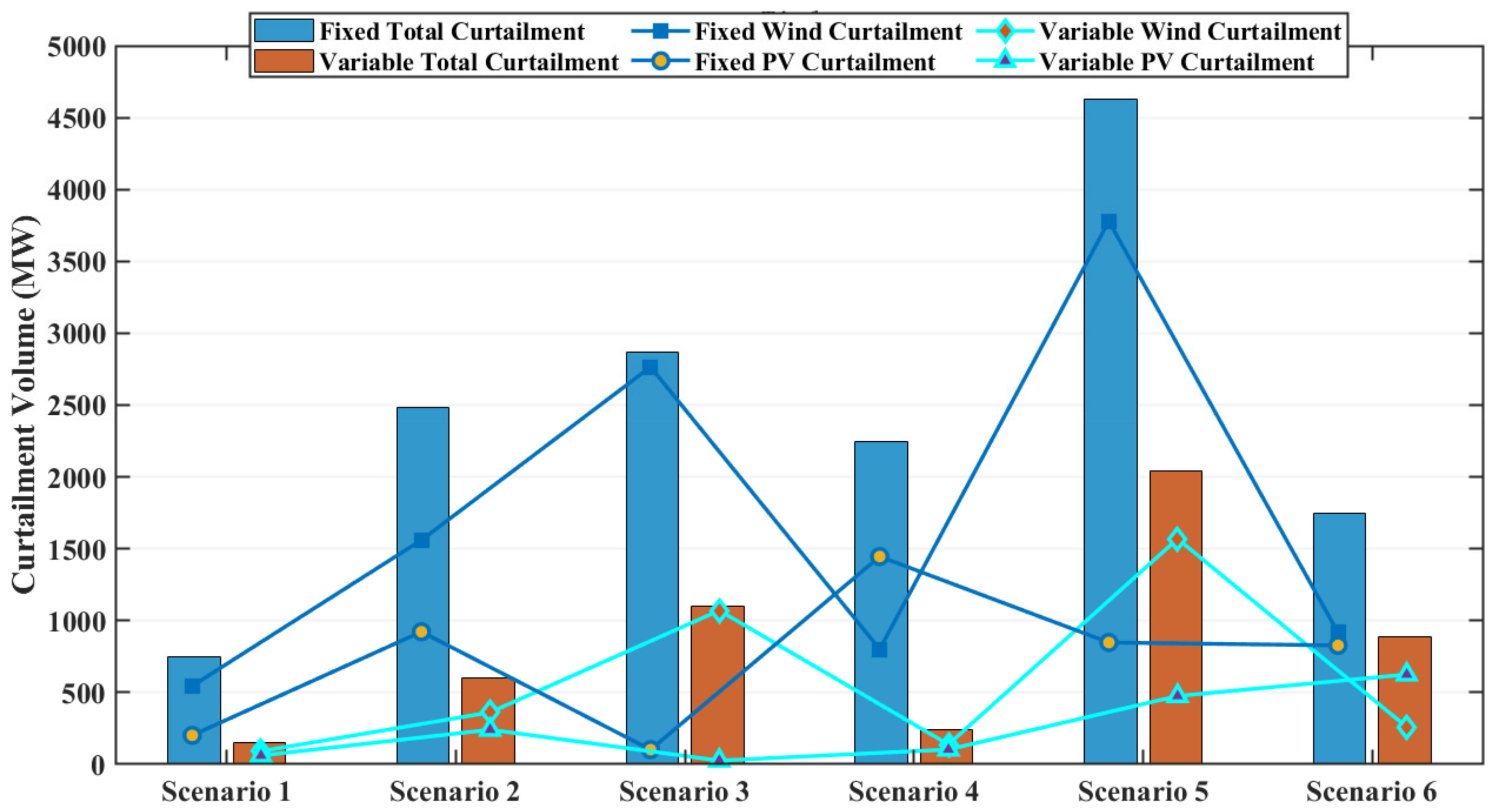
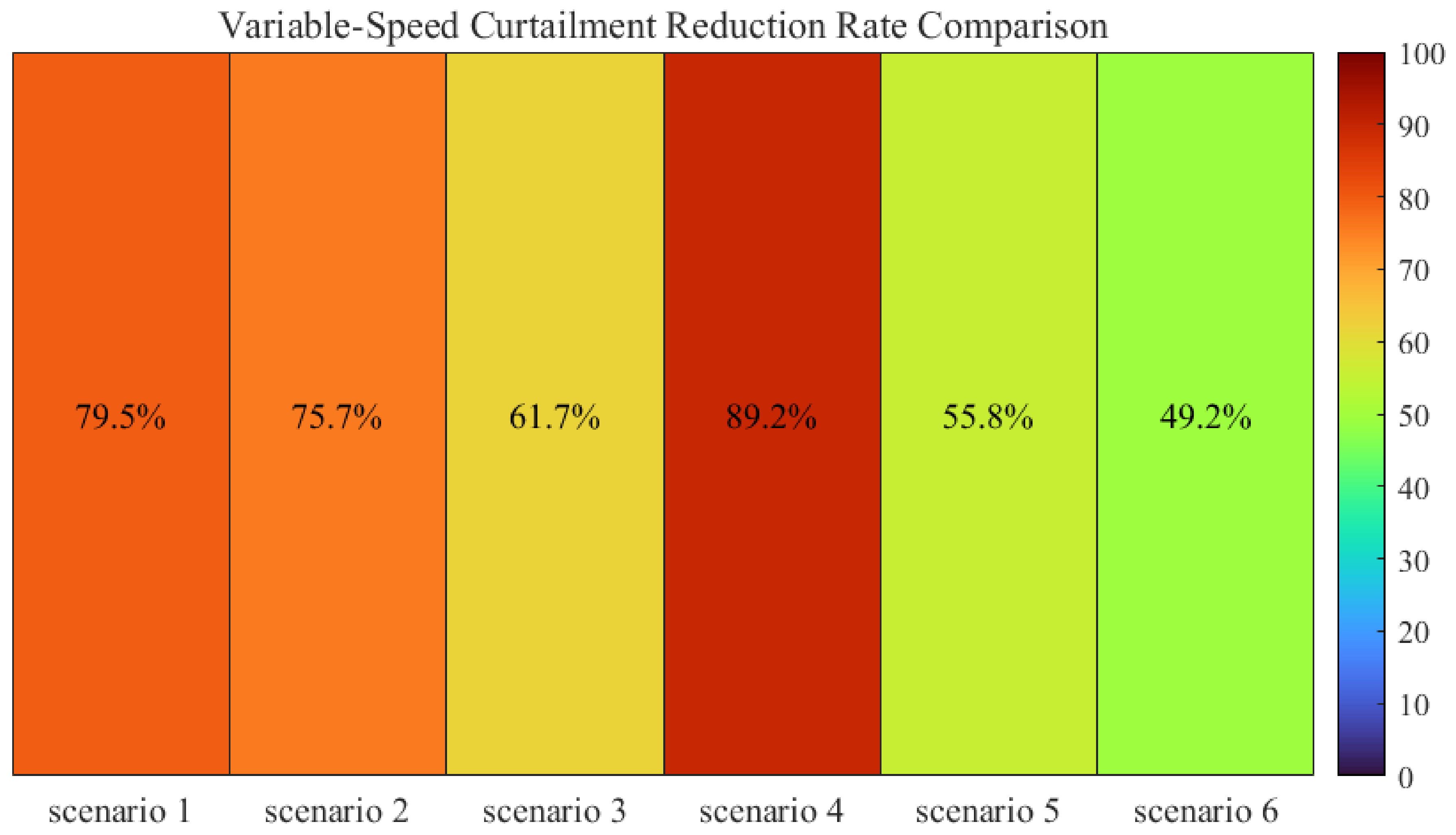
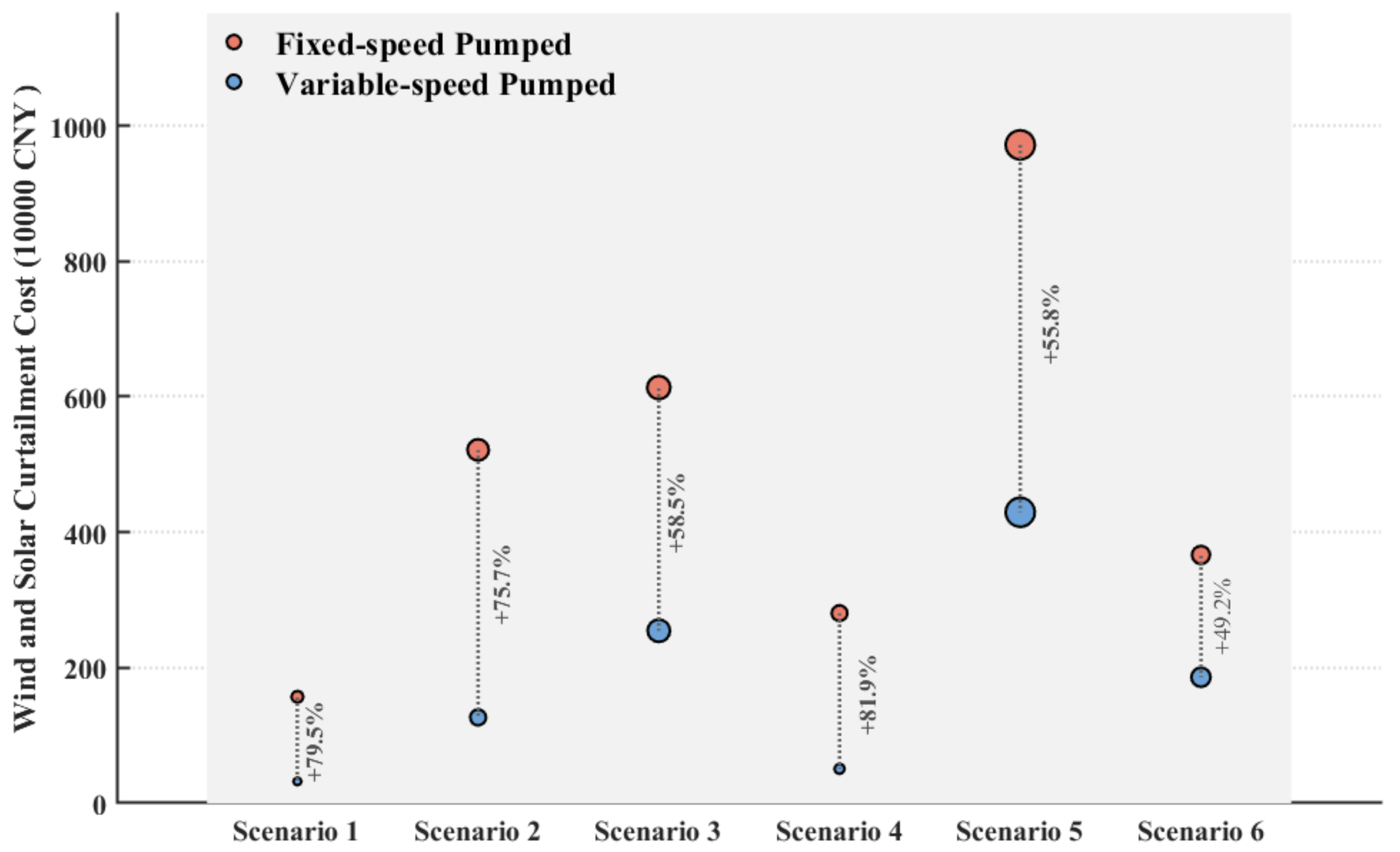
5.3. Wind and PV Curtailment Analysis

Reducing loss of wind and light energy will help increase the proportion of wind power generation in the energy structure and promote the transformation of the energy structure to green and low-carbon. As a key energy storage technology to cope with the problem of lost wind and light power, pumped storage power plants play an important role in promoting new energy consumption. In order to reduce the phenomenon of wind and light power loss and improve the capacity of new energy consumption, we have analyzed in detail the differences between VS-PS and FS-PS in terms of wind and light power consumption.
The operational flexibility of VS-PS units originates from their unique doubly-fed motor structure, enabling independent regulation of active and reactive power in both pumping and generating modes. By dynamically adjusting rotational speed within ±10% of rated speed, VS-PS units respond rapidly to grid frequency fluctuations. Compared to FS-PS units limited to fixed-rated capacity outputs, VS-PS units demonstrate extended power regulation ranges: 70–105% of rated capacity in pumping mode and 20–80% in generating mode. Particularly during sudden surges in renewable energy output such as wind and PV, VS-PS units effectively absorb excess electricity through reverse pumping, enhancing grid stability and renewable accommodation capacity. Comparative analysis in Figure 8 and Figure 9 reveals VS-PS units’ superior technical advantages in renewable energy integration. In Scenarios 1, 2, and 4, their continuously adjustable power regulation enables precise tracking of intermittent renewable generation, achieving remarkable curtailment reductions: 79.5% in Scenario 1, 75.7% in Scenario 2, and 89.2% in Scenario 4. Even in Scenarios 3, 5, and 6 with more substantial volatility, VS-PS units maintain approximately 50% curtailment mitigation effectiveness while effectively smoothing power fluctuations. This demonstrates that VS-PS units provide critical technical support for high-penetration renewable energy systems through their wide-range power regulation capabilities, substantially reducing renewable curtailment and enhancing system stability compared to conventional FS-PS units.

5.4. Operating Cost Analysis

The flexible regulation capability of VS-PS units enables valley-period charging and peak-period discharging, balancing grid load while reducing dependence on costly peak-shaving power sources, thereby lowering system operational costs. Furthermore, these units effectively mitigate wind and PV curtailment, enhance renewable energy integration capacity, and reduce associated economic losses. This study focuses on two critical components of integrated operational costs: penalty costs from renewable curtailment and coal-fired power generation costs.
As illustrated in Figure 10, VS-PS units demonstrate significant technical advantages in renewable energy integration through their flexible power regulation capabilities. Specifically, in Scenarios 1, 2, and 4, dynamic adjustments of charging/discharging power reduce wind and PV curtailment costs by 79% compared to conventional systems. In Scenarios 3, 5, and 6, an average cost reduction of 54.5% is achieved. Comprehensive analysis across all six Scenarios reveals that VS-PS systems reduce overall renewable curtailment costs by 62.3%. This empirical data validates VS-PS technology as a key research direction for addressing renewable energy uncertainty.
As shown in Figure 11, VS-PS significantly reduces renewable curtailment costs compared to FS-PS. Through flexible charging/discharging power adjustment, VS-PS effectively mitigates wind and PV curtailment by storing excess renewable generation during oversupply periods and releasing stored energy during shortages, ensuring optimal energy utilization. While Figure 11 indicates no substantial reduction in coal-fired power costs due to limited renewable penetration, VS-PS still alleviates peak-shaving pressure on thermal power and marginally lowers coal consumption compared to FS-PS. The operational inflexibility of FS-PS—fixed charging/discharging power—limits its responsiveness to grid load and renewable fluctuations, leading to increased thermal power output and reduced renewable integration. Consequently, VS-PS enhances renewable accommodation and improves power system economics and environmental benefits through optimized operational strategies.

6. Conclusions and Future Work

6.1. Conclusions

In response to the challenges posed by the increased integration of renewable energy into the power system, such as decreased scheduling stability, increased pressure on thermal power peak shaving, and carbon emission control difficulties, this study develops a day-ahead optimization scheduling model for a wind–PV–thermal–pumped storage multi-energy integrated system, based on a pumped storage power station. The goal is to achieve multi-objective collaborative control of operational costs, carbon emissions, and thermal power output fluctuations through coordinated optimization of generation and load.
(1)
This paper establishes a data-driven scenario construction and classification model and proposes an annual operational scenario division method based on the mean shift clustering algorithm. The clustering algorithm divides 280 days of wind–PV output data into six typical scenario sets. Compared to traditional manual classification methods, this approach enhances credibility and reduces subjectivity.
(2)
A three-dimensional objective function system, including operational costs, carbon emissions, and thermal power output volatility, was developed. A pumped storage station was introduced as a flexible regulation unit to enhance the stability of the integrated energy system.
(3)
This paper proposes an improved nonlinear MOJS. This algorithm significantly improves convergence accuracy and the distribution of the Pareto front by introducing a dynamic adaptive mechanism and a local search mechanism. After 500 iterations, the Pareto front convergence index (GD) of IMOJS is 0.000245, which is better than MOJS (0.00118) and NSGA-III (0.000364), demonstrating stronger convergence performance. Moreover, IMOJS shows an overall performance improvement of 17% in the three-objective optimization problem in six different test scenarios.
(4)
The introduction of VS-PS plants effectively mitigates fluctuations in thermal power output and significantly reduces joint dispatch operating costs. Through the flexible power regulation of the VS-PS plants, wind and PV curtailment costs were reduced by an average of 62.3%, effectively increasing the stability of the joint dispatch system.
This study not only provides improved algorithmic support in the field of multi-objective optimization but also demonstrates significant application value in energy dispatch and decision-making optimization. The optimized scheduling of VS-PS plants reduces fluctuations in thermal power output, enhances system reliability, and simultaneously lowers operational costs and carbon emissions, offering a practical technical pathway for a low-carbon economic transition. Looking ahead, with advancements in innovative technologies and big data analytics, intelligent energy systems based on such algorithms will address complex energy dispatch challenges with greater flexibility and efficiency. This progress will further promote the widespread adoption of green energy and facilitate the realization of sustainable development.

6.2. Future Work

This paper focuses on the generation side, but further in-depth research is needed in the following areas:
(1)
The current study only considers variable-speed pumped storage as flexible regulation units on the power supply side. Future work should incorporate the uncertainty of renewable energy forecasting by establishing wind/PV prediction models that align with their generation characteristics. Subsequent research should develop rolling optimization models for renewable energy prediction and construct multi-timescale integrated energy scheduling models to reduce uncertainties and enhance grid stability.
(2)
The current fixed electricity pricing strategy obtains optimal time-of-use pricing through calculation. Future studies could develop real-time pricing strategies based on wind power characteristics while considering long-term regional load demand with refined user load classification. More precise demand response mechanisms can be achieved by conducting an in-depth analysis of user electricity consumption behavior to improve system economic efficiency and renewable energy utilization.

Author Contributions

Y.H. (First Author): Conceptualization, Methodology, Software, Investigation, Formal Analysis, Writing—Original Draft; K.Z. (Corresponding Author): Conceptualization, Funding Acquisition, Resources, Supervision, Writing—Review and Editing; S.L.: Visualization, Investigation; Z.W.: Resources, Supervision. All authors have read and agreed to the published version of the manuscript.

Funding

This work is supported by the PhD Research Start-Up Foundation of Hubei University of Technology (No. BSDQ2020023).

Data Availability Statement

The meteorological data in this paper are from the Belgium Elia Group.

Conflicts of Interest

The authors declare that they have no conflicts of interest.

Abbreviations

AbbreviationFull Name
IMOJSImproved Multi-Objective Jellyfish Search Algorithm
LFCLoad Frequency Control
PVPhotovoltaic
KDEKernel Density Estimation
MOJSMulti-Objective Jellyfish Search Algorithm
MCAMusical Chairs Algorithm
BMCABinary version Musical Chairs Algorithm
NESTPSONested Particle Swarm Optimization
JSAThe single-objective Jellyfish Search Algorithm
MOEA/DMulti-Objective Evolutionary Algorithm based on Decomposition
SPEA2The Strength Pareto Evolutionary Algorithm 2
HVHypervolume
GDGenerational Distance
IGDInverted Generational Distance
NSGA-IIINon-dominated Sorting Genetic Algorithm III
VS-PSVariable-Speed Pumped Storage
FS-PSFixed-Speed Pumped Storage
TOPSISTechnique for Order of Preference by Similarity to Ideal Solution

Appendix A

Table A1. Comparison of IMOJS, NSGA-III, MOJS, MOEA/D and SPEA2 on the HV metric.
Test FunctionObjectivesIterationsIMOJSNSGA-IIIMOJSMOEA/DSPEA2
DTLZ133008.41 × 10−18.39 × 10−18.30 × 10−18.40 × 10−18.38 × 10−1
8.39 × 10−18.17 × 10−18.28 × 10−18.38 × 10−18.37 × 10⁻¹
8.39 × 10−18.17 × 10−18.25 × 10−18.28 × 10−18.35 × 10⁻¹
55009.69 × 10−19.70 × 10−19.64 × 10−19.68 × 10−19.58 × 10−1
9.63 × 10−19.53 × 10−19.18 × 10−19.60 × 10−19.55 × 10⁻¹
9.60 × 10−19.05 × 10−19.18 × 10−19.56 × 10−19.53 × 10⁻¹
88009.86 × 10−18.31 × 10−19.44 × 10−19.69 × 10−10.00 × 100
9.69 × 10−16.47 × 10−19.16 × 10−19.63 × 10−10.00 × 100
9.38 × 10−15.94 × 10−18.88 × 10−19.25 × 10−10.00 × 100
DTLZ233005.59 × 10−15.61 × 10−15.56 × 10−15.62 × 10−15.55 × 10−1
5.59 × 10−15.29 × 10−15.56 × 10−15.57 × 10−15.53 × 10⁻¹
5.59 × 10−15.28 × 10−15.55 × 10−15.54 × 10−15.50 × 10⁻¹
55007.78 × 10−17.75 × 10−17.68 × 10−17.76 × 10−16.70 × 10−1
7.78 × 10−17.81 × 10−17.66 × 10−17.74 × 10−16.65 × 10⁻¹
7.77 × 10−17.71 × 10−17.66 × 10−17.73 × 10−16.40 × 10⁻¹
88009.14 × 10−18.68 × 10−17.86 × 10−18.65 × 10−10.00 × 100
8.79 × 10−18.67 × 10−17.84 × 10−18.64 × 10−10.00 × 100
8.65 × 10−18.59 × 10−17.81 × 10−18.63 × 10−10.00 × 100
DTLZ333003.94 × 10−13.35 × 10−13.62 × 10−13.61 × 10−15.07 × 10−1
3.81 × 10−13.22 × 10−23.56 × 10−12.77 × 10−13.40 × 10⁻¹
2.90 × 10−13.20 × 10−12.45 × 10−11.73 × 10−13.19 × 10⁻¹
55004.46 × 10−13.80 × 10−14.26 × 10−17.08 × 10−14.26 × 10−1
4.27 × 10−13.68 × 10−13.78 × 10−13.92 × 10−14.19 × 10⁻²
3.88 × 10−13.33 × 10−13.53 × 10−11.48 × 10−12.15 × 10⁻²
88005.36 × 10−13.64 × 10−11.76 × 10−16.39 × 10−10.00 × 100
4.69 × 10−12.79 × 10−11.29 × 10−14.24 × 10−10.00 × 100
3.92 × 10−12.18 × 10−18.26 × 10−29.44 × 10−20.00 × 100
DTLZ433005.63 × 10−15.18 × 10−15.00 × 10−15.59 × 10−15.48 × 10−1
5.52 × 10−15.16 × 10−14.91 × 10−14.40 × 10−14.39 × 10⁻¹
5.15 × 10−14.93 × 10−14.85 × 10−13.41 × 10−13.47 × 10⁻¹
55007.48 × 10−17.44 × 10−17.35 × 10−16.80 × 10−16.56 × 10−1
7.46 × 10−17.34 × 10−17.32 × 10−15.69 × 10−16.18 × 10⁻¹
7.35 × 10−17.24 × 10−17.27 × 10−15.15 × 10−15.99 × 10⁻¹
88008.38 × 10−18.27 × 10−18.32 × 10−17.79 × 10−10.00 × 100
8.29 × 10−17.14 × 10−18.30 × 10−17.31 × 10−10.00 × 100
8.27 × 10−13.84 × 10−14.77 × 10−16.96 × 10−10.00 × 100
DTLZ533002.00 × 10−11.99 × 10−11.95 × 10−11.83 × 10−11.99 × 10−1
1.94 × 10−11.98 × 10−11.95 × 10−11.82 × 10−11.97 × 10⁻¹
1.93 × 10−11.93 × 10−11.94 × 10−11.77 × 10−11.84 × 10⁻¹
55001.16 × 10−11.04 × 10−11.09 × 10−11.14 × 10−14.09 × 10−2
1.14 × 10−11.03 × 10−11.07 × 10−11.13 × 10−13.54 × 10⁻²
1.15 × 10−11.02 × 10−11.04 × 10−11.07 × 10−12.07 × 10⁻²
88009.19 × 10−28.49 × 10−28.99 × 10−29.03 × 10−20.00 × 100
9.14 × 10−28.33 × 10−28.97 × 10−28.92 × 10−20.00 × 100
9.12 × 10−27.91 × 10−28.95 × 10−28.47 × 10−20.00 × 100
DTL633001.99 × 10−11.98 × 10−11.94 × 10−11.89 × 10−11.94 × 10−1
1.98 × 10−11.96 × 10−11.94 × 10−11.82 × 10−11.90 × 10⁻¹
1.92 × 10−11.91 × 10−11.94 × 10−11.76 × 10−11.79 × 10⁻¹
55001.15 × 10−18.18 × 10−28.68 × 10−21.19 × 10−19.62 × 10−2
1.14 × 10−17.61 × 10−28.57 × 10−21.12 × 10−16.77 × 10⁻²
1.11 × 10−17.49 × 10−28.01 × 10−21.03 × 10−15.40 × 10⁻²
88009.12 × 10−24.39 × 10−25.47 × 10−29.10 × 10−20.00 × 100
9.10 × 10−23.94 × 10−25.17 × 10−29.01 × 10−20.00 × 100
9.02 × 10−23.65 × 10−23.98 × 10−28.76 × 10−20.00 × 100
Table A2. Comparison of IMOJS, NSGA-III, MOJS, MOEA/D and SPEA2 based on GD.
Test FunctionObjectivesIterationsIMOJSNSGA-IIIMOJSMOEA/DSPEA2
DTLZ133003.25 × 10−47.45 × 10−46.33 × 10−27.52 × 10−45.45 × 10−4
2.80 × 10−44.46 × 10−41.22 × 10−23.58 × 10−43.84 × 10⁻⁴
2.45 × 10−43.64 × 10−41.18 × 10−32.53 × 10−43.62 × 10⁻⁴
55001.69 × 10−36.66 × 10−21.50 × 10−11.70 × 10−35.42 × 10−2
1.68 × 10−36.00 × 10−21.40 × 10−11.70 × 10−32.98 × 10⁻²
1.68 × 10−35.50 × 10−28.51 × 10−31.70 × 10−37.00 × 10⁻³
88005.29 × 10−21.07 × 10¹9.86 × 10−18.00 × 10−24.25 × 10¹
3.75 × 10−29.04 × 1009.51 × 10−17.03 × 10−24.01 × 10¹
3.56 × 10−27.54 × 1007.75 × 10−16.43 × 10−23.89 × 10¹
DTLZ233005.06 × 10−41.31 × 10−36.29 × 10−45.09 × 10−41.11 × 10−3
5.05 × 10−41.24 × 10−35.98 × 10−45.06 × 10−41.07 × 10⁻³
5.03 × 10−41.23 × 10−35.76 × 10−45.02 × 10−49.39 × 10⁻⁴
55005.25 × 10−31.26 × 10−25.44 × 10−35.40 × 10−31.74 × 10−2
5.23 × 10−31.24 × 10−25.44 × 10−35.36 × 10−31.65 × 10⁻²
5.20 × 10−31.19 × 10−25.44 × 10−35.30 × 10−31.51 × 10⁻²
88001.29 × 10−22.25 × 10−22.59 × 10−12.40 × 10−22.85 × 10−1
1.29 × 10−22.18 × 10−22.55 × 10−12.39 × 10−22.84 × 10⁻¹
2.21 × 10−21.24 × 10−22.55 × 10−12.39 × 10−22.82 × 10⁻¹
DTLZ333001.26 × 10−11.42 × 10−14.08 × 10−14.87 × 10−13.54 × 10−1
1.25 × 10−11.37 × 10−13.50 × 10−11.81 × 10−12.51 × 10⁻¹
4.27 × 10−35.32 × 10−23.01 × 10−11.19 × 10−11.15 × 10⁻¹
55003.65 × 10−14.25 × 10−19.06 × 1003.78 × 10−11.29 × 10¹
3.16 × 10−14.10 × 10−18.98 × 1003.18 × 10−15.92 × 100
2.86 × 10−13.25 × 10−18.24 × 1002.97 × 10−12.72 × 100
88002.96 × 1008.71 × 1003.10 × 1023.64E × 1022.42 × 102
2.45 × 1006.64 × 1002.93 × 1022.63 × 1022.36 × 102
2.34 × 1006.45 × 1001.93 × 1021.83 × 1022.28 × 102
DTLZ433004.75 × 10−45.47 × 10−41.32 × 10−35.07 × 10−41.27 × 10−3
4.62 × 10−44.96 × 10−41.23 × 10−34.81 × 10−41.10 × 10⁻³
4.41 × 10−44.96 × 10−41.23 × 10−34.64 × 10−41.06 × 10⁻³
55005.10 × 10−35.15 × 10−31.23 × 10−25.61 × 10−32.84 × 10−2
4.96 × 10−35.09 × 10−31.23 × 10−25.47 × 10−32.16 × 10⁻²
4.93 × 10−34.83 × 10−31.22 × 10−25.30 × 10−37.30 × 10⁻³
88001.51 × 10−21.52 × 10−22.68 × 10−12.12 × 10−22.87 × 10−1
1.43 × 10−21.40 × 10−22.67 × 10−11.77 × 10−22.84 × 10⁻¹
1.37 × 10−21.40 × 10−22.65 × 10−11.60 × 10−22.82 × 10⁻¹
DTLZ533002.40 × 10−42.79 × 10−42.74 × 10−42.40 × 10−42.62 × 10−4
2.39 × 10−42.37 × 10−42.60 × 10−42.35 × 10−42.41 × 10⁻⁴
2.38 × 10−42.36 × 10−42.48 × 10−42.27 × 10−42.11 × 10⁻⁴
55008.99 × 10−29.49 × 10−21.85 × 10−11.05 × 10−12.06 × 10−1
8.54 × 10−29.36 × 10−21.84 × 10−19.39 × 10−22.01 × 10⁻¹
8.54 × 10−29.01 × 10−21.81 × 10−18.63 × 10−21.92 × 10⁻¹
88001.38 × 10−11.70 × 10−12.78 × 10−12.73 × 10−13.20 × 10−1
1.35 × 10−11.68 × 10−12.77 × 10−12.35 × 10−13.17 × 10⁻¹
1.34 × 10−11.67 × 10−12.77 × 10−12.12 × 10−13.14 × 10⁻¹
DTL633004.76 × 10−65.05 × 10−64.63 × 10−67.15 × 10−65.15 × 10−6
4.62 × 10−65.00 × 10−64.55 × 10−65.42 × 10−64.96 × 10⁻⁶
4.48 × 10−64.95 × 10−64.51 × 10−64.95 × 10−64.57 × 10⁻⁶
55003.11 × 10−13.40 × 10−13.40 × 10−13.58 × 10−11.06 × 100
3.10 × 10−13.20 × 10−18.70 × 10−13.50 × 10−18.81 × 10⁻¹
3.09 × 10−13.03 × 10−18.69 × 10−13.12 × 10−16.39 × 10⁻¹
88004.75 × 10−14.72 × 10−11.17 × 1004.95 × 10−11.28 × 100
4.52 × 10−14.70 × 10−11.16 × 1004.92 × 10−11.21 × 100
4.48 × 10−14.56 × 10−11.14 × 1004.87 × 10−11.17 × 100
Table A3. IGD metric comparison of IMOJS, NSGA-III, MOJS, MOEA/D, and SPEA2.
Test FunctionObjectivesIterationsIMOJSNSGA-IIIMOJSMOEA/DSPEA2
DTLZ133002.09 × 10−23.73 × 10−22.85 × 10−22.18 × 10−22.21 × 10−2
2.08 × 10−22.85 × 10−22.57 × 10−22.10 × 10−22.14 × 10⁻²
2.04 × 10−22.69 × 10−22.46 × 10−22.06 × 10−22.12 × 10⁻²
55006.89 × 10−28.44 × 10−18.37 × 10−26.90 × 10−29.15 × 10−2
6.85 × 10−25.02 × 10−17.37 × 10−26.89 × 10−28.81 × 10⁻²
6.84 × 10−23.90 × 10−17.35 × 10−26.80 × 10−28.12 × 10⁻²
88001.34 × 10−11.81 × 10−11.99 × 1001.64 × 10−12.38 × 10²
1.15 × 10−11.67 × 10−11.72 × 1001.17 × 10−11.66 × 10²
1.12 × 10−11.57 × 10−11.33 × 1001.14 × 10−11.29 × 10²
DTLZ233008.98 × 10−25.66 × 10−27.08 × 10−25.49 × 10−25.76 × 10−2
5.45 × 10−25.62 × 10−26.93 × 10−25.47 × 10−25.69 × 10⁻²
5.45 × 10−25.58 × 10−26.80 × 10−25.46 × 10−25.59 × 10⁻²
55002.19 × 10−12.18 × 10−12.61 × 10−12.19 × 10−12.70 × 10−1
2.15 × 10−12.17 × 10−12.57 × 10−12.17 × 10−12.60 × 10⁻¹
2.12 × 10−12.15 × 10−12.54 × 10−12.13 × 10−12.58 × 10⁻¹
88004.42 × 10−15.43 × 10−12.15 × 1004.89 × 10−12.50 × 100
4.22 × 10−15.34 × 10−11.98 × 1004.87 × 10−12.48 × 100
4.12 × 10−14.07 × 10−11.92 × 1004.79 × 10−12.43 × 100
DTLZ333002.80 × 10−13.97 × 10−14.02 × 10−14.18 × 1007.99 × 10−1
2.29 × 10−12.40 × 10−12.75 × 10−11.00 × 1002.71 × 10−1
1.27 × 10−12.31 × 10−12.73 × 10−11.65 × 10−11.97 × 10⁻¹
55005.13 × 10−11.41 × 1001.57 × 10¹2.45 × 1009.30 × 100
4.22 × 10−19.67 × 10−11.06 × 10¹7.66 × 10−15.31 × 100
3.95 × 10−15.99 × 10−18.12 × 1005.91 × 10−12.15 × 100
88002.45 × 1003.87 × 1008.30 × 1025.84 × 1001.72 × 103
1.92 × 1003.02 × 1006.87 × 1025.71 × 1001.56 × 103
1.56 × 1002.07 × 1006.59 × 1025.67 × 1001.23 × 103
DTLZ433007.28 × 10−22.01 × 10−12.13 × 10−15.41 × 10−15.40 × 10−1
6.98 × 10−21.52 × 10−11.57 × 10−14.57 × 10−12.16 × 10⁻¹
6.82 × 10−21.03 × 10−11.04 × 10−19.57 × 10−22.01 × 10⁻¹
55002.43 × 10−12.57 × 10−13.12 × 10−16.46 × 10−14.28 × 10−1
2.34 × 10−12.56 × 10−13.03 × 10−14.03 × 10−13.68 × 10⁻¹
2.24 × 10−12.23 × 10−13.00 × 10−13.04 × 10−12.68 × 10⁻¹
88004.96 × 10−15.32 × 10−12.03 × 1006.82 × 10−12.56 × 100
4.87 × 10−14.97 × 10−11.94 × 1006.20 × 10−12.50 × 100
4.73 × 10−14.92 × 10−11.93 × 1005.79 × 10−12.42 × 100
DTLZ533006.50 × 10−31.32 × 10−21.17 × 10−23.39 × 10−26.64 × 10−3
6.41 × 10−31.24 × 10−21.08 × 10−23.38 × 10−26.18 × 10⁻³
6.35 × 10−31.18 × 10−21.06 × 10−23.37 × 10−25.97 × 10⁻³
55001.04 × 10−11.18 × 10−11.17 × 10−12.65 × 10−12.72 × 10−1
1.03 × 10−11.17 × 10−11.05 × 10−12.57 × 10−12.49 × 10⁻¹
9.89 × 10−21.06 × 10−11.04 × 10−12.52 × 10−12.13 × 10⁻¹
88002.73 × 10−12.80 × 10−12.98 × 10−12.87 × 10−12.47 × 100
2.58 × 10−12.63 × 10−12.97 × 10−12.79 × 10−12.45 × 100
2.54 × 10−12.45 × 10−12.76 × 10−12.72 × 10−12.43 × 100
DTL633006.55 × 10−32.00 × 10−21.48 × 10−23.39 × 10−27.32 × 10−3
6.53 × 10−31.89 × 10−21.39 × 10−23.38 × 10−26.89 × 10⁻³
6.52 × 10−31.86 × 10−21.35 × 10−23.29 × 10−26.84 × 10⁻³
55003.25 × 10−13.44 × 10−13.62 × 1003.51 × 10−15.41 × 100
2.85 × 10−13.25 × 10−13.57 × 1002.99 × 10−24.64 × 100
2.78 × 10−12.64 × 10−13.37 × 1002.57 × 10−23.38 × 100
88007.09 × 10−17.06 × 10−15.97 × 1007.21 × 10−11.10 × 10¹
6.69 × 10−16.98 × 10−15.71 × 1006.88 × 10−11.00 × 10¹
6.28 × 10−16.96 × 10−15.60 × 1006.35 × 10−19.99 × 100

References

  1. Guo, Y.T.; Xiang, Y. Cost-benefit analysis of PV-storage investment in integrated energy systems. Energy Rep. 2022, 8, 66–71. [Google Scholar] [CrossRef]
  2. Kocaman, A.S.; Modi, V. Value of pumped hydro storage in a hybrid energy generation and allocation system. Appl. Energy 2017, 205, 1202–1215. [Google Scholar] [CrossRef]
  3. Koholé, Y.W.; Wankouo Ngouleu, C.A.; Fohagui, F.C.V.; Tchuen, G. A comprehensive comparison of battery, hydrogen, pumped-hydro and thermal energy storage technologies for hybrid renewable energy systems integration. J. Energy Storage 2024, 93, 112299. [Google Scholar] [CrossRef]
  4. Benato, A.; Stoppato, A. Pumped Thermal Electricity Storage: A technology overview. Therm. Sci. Eng. Prog. 2018, 6, 301–315. [Google Scholar] [CrossRef]
  5. Klumpp, F. Comparison of pumped hydro, hydrogen storage and compressed air energy storage for integrating high shares of renewable energies—Potential, cost-comparison and ranking. J. Energy Storage 2016, 8, 119–128. [Google Scholar] [CrossRef]
  6. Xu, B.; Chen, D.; Venkateshkumar, M.; Xiao, Y.; Yue, Y.; Xing, Y.; Li, P. Modeling a pumped storage hydropower integrated to a hybrid power system with PV-wind power and its stability analysis. Appl. Energy 2019, 248, 446–462. [Google Scholar] [CrossRef]
  7. Naval, N.; Yusta, J.M.; Sánchez, R.; Sebastián, F. Optimal scheduling and management of pumped hydro storage integrated with grid-connected renewable power plants. J. Energy Storage 2023, 73, 108993. [Google Scholar] [CrossRef]
  8. Hunt, J.D.; Al-Nory, M.T.; Slocum, A.H.; Wada, Y. Integrated seasonal pumped hydro, cooling, and reverse osmosis: A solution to desert coastal regions. Desalination 2025, 593, 118242. [Google Scholar] [CrossRef]
  9. Shyam, B.; Kanakasabapathy, P. Feasibility of floating PV PV integrated pumped storage system for a grid-connected microgrid under static time of day tariff environment: A case study from India. Renew. Energy 2022, 192, 200–215. [Google Scholar] [CrossRef]
  10. Liu, L.; Sun, Q.; Li, H.; Yin, H.; Ren, X.; Wennersten, R. Evaluating the benefits of Integrating Floating PV and Pumped Storage Power System. Energy Conv. Manag. 2019, 194, 173–185. [Google Scholar] [CrossRef]
  11. Bhayo, B.A.; Al-Kayiem, H.H.; Gilani, S.I.U.; Ismail, F.B. Power management optimization of hybrid PV PV-battery integrated with pumped-hydro-storage system for standalone electricity generation. Energy Conv. Manag. 2020, 215, 112942. [Google Scholar] [CrossRef]
  12. Li, J.; Zhao, Z.; Li, P.; Apel Mahmud, M.; Liu, Y.; Chen, D.; Han, W. Comprehensive benefit evaluations for integrating off-river pumped hydro storage and floating PV. Energy Conv. Manag. 2023, 296, 117651. [Google Scholar] [CrossRef]
  13. Ma, T.; Yang, H.; Lu, L.; Peng, J. Optimal design of an autonomous PV–wind-pumped storage power supply system. Appl. Energy 2015, 160, 728–736. [Google Scholar] [CrossRef]
  14. Zhao, Z.; Yuan, Y.; He, M.; Jurasz, J.; Wang, J.; Egusquiza, M.; Egusquiza, E.; Xu, B.; Chen, D. Stability and efficiency performance of pumped hydro energy storage system for higher flexibility. Renew. Energy 2022, 199, 1482–1494. [Google Scholar] [CrossRef]
  15. Liu, J.; Ma, T.; Wu, H.; Yang, H. Study on optimum energy fuel mix for urban cities integrated with pumped hydro storage and green vehicles. Appl. Energy 2023, 331, 120399. [Google Scholar] [CrossRef]
  16. Ren, Y.; Sun, K.; Zhang, K.; Han, Y.; Zhang, H.; Wang, M.; Jing, X.; Mo, J.; Zou, W.; Xing, X. Optimization of the capacity configuration of an abandoned mine pumped storage/wind/PV integrated system. Appl. Energy 2024, 374, 124089. [Google Scholar] [CrossRef]
  17. Zhu, Y.; Yao, S.; Zhang, Y.; Cao, M. Environmental and economic scheduling for wind-pumped storage-thermal integrated energy system based on priority ranking. Electr. Power Syst. Res. 2024, 231, 110353. [Google Scholar] [CrossRef]
  18. Connolly, D.; Lund, H.; Mathiesen, B.V.; Pican, E.; Leahy, M. The technical and economic implications of integrating fluctuating renewable energy using energy storage. Renew. Energy 2012, 43, 47–60. [Google Scholar] [CrossRef]
  19. Patwal, R.S.; Narang, N. Multi-objective generation scheduling of integrated energy system using fuzzy based surrogate worth trade-off approach. Renew. Energy 2020, 156, 864–882. [Google Scholar] [CrossRef]
  20. Yan, Y.; Wu, T.; Li, S.; Xie, H.; Li, Y.; Liu, M.; Zhao, Y.; Liang, H.; Zhang, G.; Xin, H. Optimal operation strategies of pumped storage hydropower plant considering the integrated AC grids and new energy utilization. Energy Rep. 2022, 8, 545–554. [Google Scholar] [CrossRef]
  21. Sun, H.; Ren, Q.; Hou, J.; Zhao, Z.; Xie, D.; Zhao, W.; Meng, F. Study on the performance and economy of the building-integrated micro-grid considering PV and pumped storage: A case study in Foshan. Int. J. Low-Carbon Technol. 2022, 17, 630–636. [Google Scholar] [CrossRef]
  22. Xu, Y.; Li, C.; Wang, Z.; Zhang, N.; Peng, B. Load Frequency Control of a Novel Renewable Energy Integrated Micro-Grid Containing Pumped Hydropower Energy Storage. IEEE Access 2018, 6, 29067–29077. [Google Scholar] [CrossRef]
  23. Xu, J.P.; Liu, T.T. Optimal Hourly Scheduling for Wind-Hydropower Systems with Integrated Pumped-Storage Technology. J. Energy Eng. 2021, 147, 04021013. [Google Scholar] [CrossRef]
  24. Pérez-Díaz, J.I.; Jiménez, J. Contribution of a pumped-storage hydropower plant to reduce the scheduling costs of an isolated power system with high wind power penetration. Energy 2016, 109, 92–104. [Google Scholar] [CrossRef]
  25. Wang, X.Y.; Bai, Y.P. The global Minmax k-means algorithm. Springerplus 2016, 5, 1665. [Google Scholar] [CrossRef]
  26. Chen, Q.Q.; He, L.J.; Diao, Y.A.; Zhang, K.B.; Zhao, G.R.; Chen, Y.M. A Novel Neighborhood Granular Meanshift Clustering Algorithm. Mathematics 2023, 11, 207. [Google Scholar] [CrossRef]
  27. Liao, Y.; Zhao, Y.; Fang, N.; Huang, J. A Study on Site Selection for Regional Air Rescue Centers Based on Multi-Objective Jellyfish Search Algorithm. Biomimetics 2023, 8, 254. [Google Scholar] [CrossRef]
  28. Wang, X.; Feng, Y.; Tang, J.; Dai, Z.; Zhao, W. A UAV path planning method based on the framework of multi-objective jellyfish search algorithm. Sci. Rep. 2024, 14, 28058. [Google Scholar] [CrossRef]
  29. Yang, B.; Yin, Y.; Gao, Y.; Wang, S.; Fu, G.; Zhou, P. Field-factory hybrid service mode and its resource scheduling method based on an enhanced MOJS algorithm. Comput. Ind. Eng. 2022, 171, 108508. [Google Scholar] [CrossRef]
  30. Tian, J.; Qian, C.Y. Improved Multi-Objective Jellyfish Search Algorithm for UAV 3D Trajectory Planning. J. Northwest Univ. Natl. (Nat. Sci.) 2024, 45, 41–55. [Google Scholar] [CrossRef]
  31. Zhang, L.; Wang, N.Y.; Mao, J.L.; Li, R.Q. Low carbon flexible job shop scheduling based on improved multi-objective jellyfish search algorithm. Mech. Electr. Eng. Mag. 2023, 40, 1086–1092. [Google Scholar] [CrossRef]
  32. Tao, X.J.; Mo, Y.B. Improved Artificial Jellyfish Search Algorithm in Equations with Multiple Roots and Engineering Application. Math. Pract. Theory 2023, 53, 160–173. [Google Scholar]
  33. Eltamaly, A.M.; Rabie, A.H. A Novel Musical Chairs Optimization Algorithm. Arab. J. Sci. Eng. 2023, 48, 10371–10403. [Google Scholar] [CrossRef]
  34. Eltamaly, A.M. A Novel Strategy for Optimal PSO Control Parameters Determination for PV Energy Systems. Sustainability 2021, 13, 1008. [Google Scholar] [CrossRef]
  35. Ma, L.; Wang, Z.; Lu, Z.; Lu, X.; Wan, F. Integrated Strategy of the Output Planning and Economic Operation of the Combined System of Wind Turbines-Pumped-Storage-Thermal Power Units. IEEE Access 2019, 7, 20567–20576. [Google Scholar] [CrossRef]
  36. Liu, P.; Wu, X.; Wang, Z.; Bo, Y.; Bao, H. Numerical simulation study on gas-solid flow characteristics and SO2 removal characteristics in circulating fluidized bed desulfurization tower. Chem. Eng. Process.-Process Intensif. 2022, 176, 108974. [Google Scholar] [CrossRef]
  37. Meng, Z.; Wang, C.; Wang, X.; Chen, Y.; Wu, W.; Li, H. Simultaneous removal of SO2 and NOx from flue gas using (NH4)2S2O3/steel slag slurry combined with ozone oxidation. Fuel 2019, 255, 115760. [Google Scholar] [CrossRef]
  38. Lyu, X.; Liu, T.Q.; Liu, X.; He, C.; Nan, L.; Zeng, H. Low-carbon robust economic dispatch of park-level integrated energy system considering price-based demand response and vehicle-to-grid. Energy 2023, 263, 125739. [Google Scholar] [CrossRef]
  39. Yang, Y.; Wei, Q.Y.; Liu, S.K.; Zhao, L. Distribution Strategy Optimization of Standalone Hybrid WT/PV System Based on Different PV and Wind Resources for Rural Applications. Energies 2022, 15, 5307. [Google Scholar] [CrossRef]
  40. Zhao, P.Y.; Nan, H.P.; Cai, Q.S.; Gao, C.Y.; Wu, L.C. A Data-Driven Predictive Control Method for Modeling Doubly-Fed Variable-Speed Pumped Storage Units. Energies 2024, 17, 4912. [Google Scholar] [CrossRef]
  41. Shi, Y.F.; Shi, X.J.; Yi, C.B.; Song, X.F.; Chen, X.G. Control of the Variable-Speed Pumped Storage Unit-Wind Integrated System. Math. Probl. Eng. 2020, 2020, 3816752. [Google Scholar] [CrossRef]
Figure 1. Silhouette coefficient value plot for samples.
Energies 18 02308 g001
Figure 2. Clustering data of wind–PV scenarios.
Energies 18 02308 g002
Figure 3. Wind and PV power output curves.
Energies 18 02308 g003aEnergies 18 02308 g003b
Figure 4. The flowchart of the improved jellyfish algorithm.
Energies 18 02308 g004
Figure 5. Wind–PV–thermal–pumped storage integrated scheduling model.
Energies 18 02308 g005
Figure 6. Process flowchart based on the multi-objective jellyfish algorithm.
Energies 18 02308 g006
Figure 7. VS-PS and FS-PS joint dispatch output diagrams.
Energies 18 02308 g007aEnergies 18 02308 g007b
Figure 8. Comparison of curtailment volume between VS-PS and FS-PS.
Energies 18 02308 g008
Figure 9. VS-PS curtailment reduction rate comparison.
Energies 18 02308 g009
Figure 10. Wind and PV curtailment costs.
Energies 18 02308 g010
Figure 11. Coal fuel cost for thermal power.
Energies 18 02308 g011
Table 1. Survey of previous studies.
ReferenceVS-PSWind–PV Data PreprocessingAlgorithm ImprovementLarge-Scale Power Generation System
[7]×××
[8]××
[9]×××
[10]××××
[12]××
[13]×××
[14]××
[15]××
[16]×××
[17]×××
[20]××
[21]×××
[23]××
Proposed
Table 2. Three metrics for evaluating clustering performance.
IndexValue
Mean Silhouette0.613
Calinski–Harabasz710.7
Davies–Bouldin0.542
Table 3. Clustered scenario division.
ScenariosClass NameDate
Scenario 1Weak Wind and Weak Light28 June 2021
Scenario 2Moderate Wind and Weak Light13 April 2021
Scenario 3Weak Wind and Strong Light19 May 2021
Scenario 4Strong Wind and Strong Light29 May 2021
Scenario 5Strong Wind and Weak Light31 March 2021
Scenario 6Moderate Wind and Strong Light26 August 2021
Table 4. Comparison of IMOJS, NSGA-III, MOJS, MOEA/D and SPEA2 on the HV metric.
Test FunctionObjectivesIterationsIMOJSNSGA-IIIMOJSMOEA/DSPEA2
DTLZ155009.69 × 10−19.70 × 1019.64 × 10−19.68 × 10−19.58 × 10−1
9.63 ×1019.53 × 10−19.18 × 10−19.60 × 10−19.55 × 10⁻¹
9.60 × 1019.05 × 10−19.18 × 10−19.56 × 10−19.53 × 10⁻¹
DTLZ233005.59 × 10−15.61 × 10−15.56 × 10−15.62 × 10−15.55 × 10−1
5.59 × 1015.29 × 10−15.56 × 10−15.57 × 10−15.53 × 10⁻¹
5.59 × 1015.28 × 10−15.55 × 10−15.54 × 10−15.50 × 10⁻¹
DTLZ333003.94 × 10−13.35 × 10−13.62 × 10−13.61 × 10−15.07 × 101
3.81 × 1013.22 × 10−13.56 × 10−12.77 × 10−13.40 × 10⁻¹
2.90 × 10−13.20 × 1012.45 × 10−11.73 × 10−13.19 × 10−1
55004.46 × 10−13.80 × 10−14.26 × 10−17.08 × 1014.26 × 10−1
4.27 × 1013.68 × 10−13.78 × 10−13.92 × 10−14.19 × 10⁻¹
3.88 × 1013.33 × 10−13.53 × 10−11.48 × 10−12.15 × 10⁻¹
88005.36 × 10−13.64 × 10−11.76 × 10−16.39 × 1010.00 × 100
4.69 × 1012.79 × 10−11.29 × 10−14.24 × 10−10.00 × 100
3.92 × 1012.18 × 10−18.26 × 10−29.44 × 10−20.00 × 100
DTLZ488008.38 × 1018.27 × 10−18.32 × 10−17.79 × 10−10.00 × 100
8.29 × 10−17.14 × 10−18.30 × 1017.31 × 10−10.00 × 100
8.27 × 1013.84 × 10−14.77 × 10−16.96 × 10−10.00 × 100
DTLZ655001.15 × 10−18.18 × 10−28.68 × 10−21.19 × 1019.62 × 10−2
1.14 × 1017.61 × 10−28.57 × 10−21.12 × 10−16.77 × 10⁻²
1.11 × 1017.49 × 10−28.01 × 10−21.03 × 10−15.40 × 10⁻²
Table 5. Comparison of IMOJS, NSGA-III, MOJS, MOEA/D and SPEA2 based on GD.
Test FunctionObjectivesIterationsIMOJSNSGA-IIIMOJSMOEA/DSPEA2
DTLZ233005.06 × 1041.31 × 10−36.29 × 1045.09 × 1041.11 × 10−3
5.05 × 1041.24 × 10−35.98 × 1045.06 × 1041.07 × 10−3
5.03 × 1041.23 × 10−35.76 × 1045.02 × 1049.39 × 104
88001.29 × 1042.25 × 10−22.59 × 1012.40 × 1022.85 × 101
1.29 × 1042.18 × 10−22.55 × 1012.39 × 1022.84 × 101
2.21 × 1041.24 × 1022.55 × 1012.39 × 1022.82 × 101
DTLZ433004.75 × 10−45.47 × 10−41.32 × 10−35.07 × 10−41.27 × 10−3
4.62 × 10−44.96 × 10−41.23 × 10−34.81 × 10−41.10 × 10⁻³
4.41 × 10−44.96 × 10−41.23 × 10−34.64 × 10−41.06 × 10⁻³
88001.51 × 10−21.52 × 10−22.68 × 10−12.12 × 10−22.87 × 10−1
1.43 × 10−21.40 × 10−22.67 × 10−11.77 × 10−22.84 × 10⁻¹
1.37 × 10−21.40 × 10−22.65 × 10−11.60 × 10−22.82 × 10⁻¹
DTL633004.76 × 10−65.05 × 10−64.63 × 10−67.15 × 10−65.15 × 10−6
4.62 × 10−65.00 × 10−64.55 × 10−65.42 × 10−64.96 × 10⁻⁶
4.48 × 10−64.95 × 10−64.51 × 10−64.95 × 10−64.57 × 10⁻⁶
55003.11 × 10−13.40 × 10−13.40 × 10−13.58 × 1011.06 × 100
3.10 × 10−13.20 × 10−18.70 × 10−13.50 × 10−18.81 × 10⁻¹
3.09 × 10−13.03 × 10−18.69 × 10−13.12 × 10−16.39 × 10⁻¹
88004.75 × 10−14.72 × 10−11.17 × 1004.95 × 10−11.28 × 100
4.52 × 10−14.70 × 10−11.16 × 1004.92 × 10−11.21 × 100
4.48 × 10−14.56 × 10−11.14 × 1004.87 × 10−11.17 × 100
Table 6. IGD metric comparison of IMOJS, NSGA-III, MOJS, MOEA/D, and SPEA2.
Test FunctionObjectivesIterationsIMOJSNSGA-IIIMOJSMOEA/DSPEA2
DTLZ233008.98 × 10−25.66 × 10−27.08 × 10−25.49 × 10−25.76 × 10−2
5.45 × 10−25.62 × 10−26.93 × 10−25.47 × 10−25.69 × 10⁻²
5.45 × 10−25.58 × 10−26.80 × 10−25.46 × 10−25.59 × 10⁻²
55002.19 × 10−12.18 × 10−12.61 × 10−12.19 × 10−12.70 × 10−1
2.15 × 10−12.17 × 10−12.57 × 10−12.17 × 10−12.60 × 10⁻¹
2.12 × 10−12.15 × 10−12.54 × 10−12.13 × 10−12.58 × 10⁻¹
88004.42 × 10−15.43 × 10−12.15 × 1004.89 × 10−12.50 × 100
4.22 × 10−15.34 × 10−11.98 × 1004.87 × 10−12.48 × 100
4.12 × 10−14.07 × 10−11.92 × 1004.79 × 10−12.43 × 100
DTLZ533006.50 × 10−31.32 × 10−21.17 × 10−23.39 × 10−26.64 × 10−3
6.41 × 10−31.24 × 10−21.08 × 10−23.38 × 10−26.18 × 10⁻³
6.35 × 10−31.18 × 10−21.06 × 10−23.37 × 10−25.97 × 10⁻³
88002.73 × 10−12.80 × 10−12.98 × 10−12.87 × 10−12.47 × 100
2.58 × 10−12.63 × 10−12.97 × 10−12.79 × 10−12.45 × 100
2.54 × 10−12.45 × 10−12.76 × 10−12.72 × 10−12.43 × 100
DTLZ655003.25 × 10−13.44 × 10−13.62 × 1003.51 × 10−15.41 × 100
2.85 × 10−13.25 × 10−13.57 × 1002.99 × 10−24.64 × 100
2.78 × 10−12.64 × 10−13.37 × 1002.57 × 10−23.38 × 100
88007.09 × 10−17.06 × 10−15.97 × 1007.21 × 10−11.10 × 10¹
6.69 × 10−16.98 × 10−15.71 × 1006.88 × 10−11.00 × 10¹
6.28 × 10−16.96 × 10−15.60 × 1006.35 × 10−19.99 × 100
Table 7. Major pollutants emitted by thermal power plants and treatment costs (per 1 ton of coal) [37,38].
PollutantsEmission/kgTreatment Cost/(CNY·kg−1)
SO21.256
NOx88
TSP0.412.20
Table 8. Experimental parameters for wind–PV–thermal–pumped storage system.
Installed Capacity of Each Power Source and Pumped Storage ParametersData
Total Capacity of the Wind Farm1500 MW
Total Capacity of the PV Power Plant1000 MW
Total Capacity of the Pumped Storage Units1200 MW
Hydroelectric Conversion Efficiency0.75
Reservoir Capacity Upper Limit2806.5 m
Reservoir Capacity Lower Limit2784 m
Total Installed Capacity of Thermal Power Plant3000 MW
a(t/MW2)0.00056
b(t/MW)0.384
c(t)2.2
Table 9. Dispatch results of different algorithms.
ScenarioAlgorithmSystem Operating Cost (Ten Thousand CNY)CO2 Emissions (t)Fluctuations in Thermal Power Generation
Scenario1IMOJS1652.425,867.3159.3
MOJS1826.427,024.5226.4
NSGA-III1718.926,202.6254.8
MOEA/D1697.226,110.4267.6
SPEA-21807.526,924.1314.5
Scenario 2IMOJS2503.638,133.7241.2
MOJS2604.738,468.3319.2
NSGA-III2567.338,294.5261.4
MOEA/D2658.938,599.1258.7
SPEA-22692.538,652.2245.3
Scenario 3IMOJS1588.219,917.4174.0
MOJS1757.920,296.5181.9
NSGA-III1692.420,158.0198.6.
MOEA/D1638.720,029.6185.3
SPEA-21782.620,379.2189.5
Scenario 4IMOJS3245.351,396.5213.6
MOJS3425.952,637.9228.4
NSGA-III3306.451,743.8224.9
MOEA/D3372.651,826.3238.7
SPEA-23406.852,489.6220.1
Scenario 5IMOJS1801.121,861.3269.2
MOJS2213.722,399.1278.3
NSGA-III1976.922,067.3294.0
MOEA/D1899.621,985.7311.8
SPEA-22344.522,518.5307.4
Scenario 6IMOJS2921.343,950.5298.7
MOJS3018.944,207.6308.4
NSGA-III2989.744,112.8352.5
MOEA/D2997.444,197.1322.2
SPEA-23242.444,814.3314.0
Table 10. Comparison of daily dispatch results for VS-PS and FS-PS in the joint operation system.
ScenarioVariable/Fixed Pumped StorageSystem Operating Cost (Ten Thousand CNY)CO2 Emissions (t)Fluctuations in Thermal Power Generation
Scenario 1Variable1652.425,867.3159.3
Fixed1867.827,338.7292.1
Scenario 2Variable2503.638,133.7241.2
Fixed2977.639,387.4333.0
Scenario 3Variable1588.219,917.4174.0
Fixed1911.220,645.3200.3
Scenario 4Variable3245.351,396.5213.6
Fixed3563.652,814.6261.0
Scenario 5Variable1801.121,861.3269.2
Fixed2400.322,764.9285.6
Scenario 6Variable2921.343,950.5298.7
Fixed3126.344,315.3338.0
Disclaimer/Publisher’s Note: The statements, opinions and data contained in all publications are solely those of the individual author(s) and contributor(s) and not of MDPI and/or the editor(s). MDPI and/or the editor(s) disclaim responsibility for any injury to people or property resulting from any ideas, methods, instructions or products referred to in the content.

