Design and Analysis of a Novel Ocean Current Two-Coupled Crossflow Turbine Energy Converter

Abstract

In this study, a novel ocean current energy converter is proposed. The energy converter is composed of two crossflow turbines. The two turbines rotate at the same speed but in opposite directions; therefore, the summation of the hydrodynamic torques applied to the two turbines is equal to zero, which can make the converter self-stabilizing. A channel is designed to guide a large amount of water flowing through the turbine, thereby increasing the incident velocity, power, and efficiency of the turbine. The guide vanes are positioned in front of the turbine to guide the ocean current, producing the optimal flow incident angle and thereby increasing the performance of the turbine. A novel empirical formula for determining the power and efficiency of the converter is derived. Moreover, a computational fluid dynamics (CFD) analysis of the energy converter is conducted using the commercial software Star CCM+ in the standard κ-ω turbulence model with wall functions. The accuracy of the empirical formula is verified by comparing the theoretical results with those obtained using the CFD method. Finally, the effects of several parameters on the performance of the energy converter are investigated. The optimal parameters are obtained as follows: (1) The optimal setting angles of vanes γ₁ = 78°, ${\gamma }_2={\gamma }_1+10°$, and ${\gamma }_3={\gamma }_1-5°$. (2) The optimal blade angle β = 44°. (3) The optimal rotating speed N = 2.6 (V_cur/1.6) rpm. (4) The optimal ratio of turbine center distance r_L4 ≥ 2.50. (5) The optimal ratio of turbine shaft length is approximately 5.5 < (r_shaft = W_shaft/D_tur)_opt < 5.7. (6) The performance of each turbine with N_blade = 31 blades is significantly better than that with N_blade = 23 blades.

1. Introduction

Ocean energy that can be harnessed by exploiting an aspect of the physical or chemical characteristics of the ocean includes (1) global ocean currents, (2) tidal currents, (3) wave motion, (4) thermal gradients, and (5) salinity gradients. A turbine is a vital device for converting energy from global ocean and tidal currents whose energy source is ocean current velocity. The direction of flow of global ocean currents is steady, but tidal currents vary [1,2].

Global ocean currents hold substantial energy potential. Taiwan is influenced by the Kuroshio Current along its eastern coastline. The estimated potential for electricity generation from the Kuroshio Current near Taiwan exceeds 10 GW during the summer months and reaches approximately 4 GW in winter. The Kuroshio Current is part of the global ocean current system. In general, the seabed beneath the Kuroshio Current is almost over 1000 m in the area mentioned above. Deep mooring technology and the self-stability of turbines are essential for harnessing this energy [2,3,4]. However, tidal power generation turbines are often installed on the seabed at a depth of less than 50 m, and the turbines can be directly fixed to the seabed using high-strength structures [5,6].

Two principal types of ocean current turbines (OCTs) have been developed to date. The first type is the translational blade turbine, characterized by blades that undergo linear reciprocating motion in the vertical direction relative to the sea surface (Figure 1a) [3]. The second type is the horizontal-axis ocean current turbine, which employs blades that rotate about a horizontal shaft aligned with the direction of the ocean current—an operational principle analogous to that of horizontal-axis tidal current turbines (Figure 1b) [2,7,8,9]. In a field demonstration, Chen et al. [4] successfully deployed a 50 kW ocean current energy converter, moored at a depth of 850 m on the seabed in the Pingtung offshore region of Taiwan. The characteristics of the translational blade OCT include (1) high efficiency, (2) complex mechanism, (3) high cost, and (4) self-stability. The blades of the first energy converter move in translational motion, like a conveyor belt. Because the blade is subjected to hydrodynamic forces, no rotating torques are applied to the converter; it is self-stabilizing. However, the mechanism is complex and expensive. The efficiency of a translational blade OCT is high because the attack angle of each blade in motion can be optimally adjusted and fixed [4]. The characteristics of the horizontal-axis rotational blade OCTs include (1) high efficiency, (2) a weak connecting structure, (3) two turbines and two generators, and (4) low dynamic stability. The efficiency is high because the blade operates effectively regardless of the rotation angle, and there is no interference between blades. The horizontal-axis OCT energy converter rotates about the horizontal axis in the same direction as the current. The converter includes two turbines that rotate at the same speed but in opposite directions so that the torque summation of the two turbines is equal to zero; therefore, it is self-stabilizing [2,7]. However, because its center of gravity is too high, the dynamic stability of the mooring system is low. The diameter of the horizontal-axis ocean turbine increases with power. The diameter of an MW-scale turbine is very large. Two turbines are connected by a beam. The distance between the two turbines must be very large to prevent them from interfering with each other; therefore, the span of the connecting beam is very long, resulting in weak bending rigidity of the beam [2]. The purpose of this study is to develop a better ocean current power turbine. A more efficient ocean current power generation method is proposed in this study based on the characteristics of tidal and traditional hydropower turbines. The literature on tidal currents and hydraulic turbines is reviewed below.

The global exploitable tidal current power based on currently available technologies is estimated to be about 75 GW [1,5,6]. In recent years, several studies have investigated the horizontal-axis tidal current turbines (TCTs) [10,11,12] and the vertical-axis ones [13,14,15]. The majority of industrialized TCT devices are horizontal-axis turbines with rotation axes parallel to the current flow direction. The main disadvantages associated with vertical-axis turbines are their relatively low self-starting capability, high torque fluctuations, and generally lower efficiency compared with horizontal-axis turbine designs. The efficiency of a horizontal-axis TCT is high because each blade operates effectively regardless of rotation angle [5,6]. The efficiency of a vertical-axis TCT is low because the relative motion of the blade in response to the current depends on the rotational angle; thus, the energy generated by the relative blade–current motion varies and may even be negative. However, power generation by vertical-axis TCTs with a symmetrical wing can be driven regardless of the flow direction.

The main component of a traditional hydropower plant is the hydraulic turbine, in which the potential energy is derived from the water head; however, the ocean current energy source is kinetic energy, i.e., current velocity. Therefore, the design of the ocean current turbine (OCT) is different from that of the hydraulic turbine. There have been several studies on the successful application of hydropower. Hydraulic turbines under high head drop conditions include Pelton, Francis, or Kaplan turbines; on the other hand, crossflow turbines (CFTs) are suitable for low head drop conditions. They can operate efficiently at various flow rates. They are simple in design, easy to manufacture, and easy to maintain and have low costs and high efficiency. The differences between traditional CFT hydroelectric turbines and vertical-axis tidal current turbines include the following: (1) The energy type of traditional hydroelectric turbines is potential energy, while the energy type of ocean and tidal current turbines is kinetic energy. (2) Traditional hydraulic turbines have many blades, while tidal current turbines generally have three blades. (3) The shape of traditional CFT hydraulic turbine blades is curved and asymmetric, while the shape of vertical-axis tidal current turbine blades is symmetrical. (4) The efficiency of the hydraulic CFT is significantly higher than that of the vertical-axis tidal current turbines (TCT).

Some studies have focused on developing an empirical formula expressing the performance and parameters of hydraulic turbines. The formula is simple and helpful for the initial design of CFT geometry. Mockmore and Merryfield [16], Sinagra et al. [17], Sinagra et al. [18], and Adanta et al. [19] investigated the relationship between the incident velocity at the inlet of the turbine and the net head. Mockmore and Merryfield [16] and Sammartano et al. [20] proposed a formula for power and efficiency. However, these empirical formulas exclude the effects of the blade angle and the inlet and outlet areas. Adanta et al. [19], Woldemariam et al. [21], and Picone et al. [22] analyzed the CFD of CFTs using the commercial software ANSYS Fluent in the standard κ-ε turbulence model. Acharya et al. [23] conducted a CFD analysis of CFT using the commercial software ANSYS CFX in the Menter shear stress transport (SST) turbulence model. Kaya et al. [24] conducted a CFD analysis of the CFT using the commercial software Star CCM+ in the standard κ-ε turbulence model with wall function.

This study presents a novel high-efficiency and self-balancing ocean current power generation turbine to improve the shortcomings of the horizontal-axis OCTs’ weak structure and poor stability. The ocean current multi-blade CFT has high efficiency and structural strength. It is a vertical-axis CFT with a low center of gravity and good stability. The ocean current multi-blade CFT is different from vertical-axis three-blade tidal current turbines. The innovative design of an ocean current converter integrates a pair of CFTs with forward and reverse rotation, which can make the entire unit self-stabilizing. In addition, theoretical formulas for accurately calculating the power and efficiency of the energy converter are provided. The effects of several parameters on performance and efficiency are also investigated using the CFD method.

2. Design of Ocean Current CFT Energy Converters

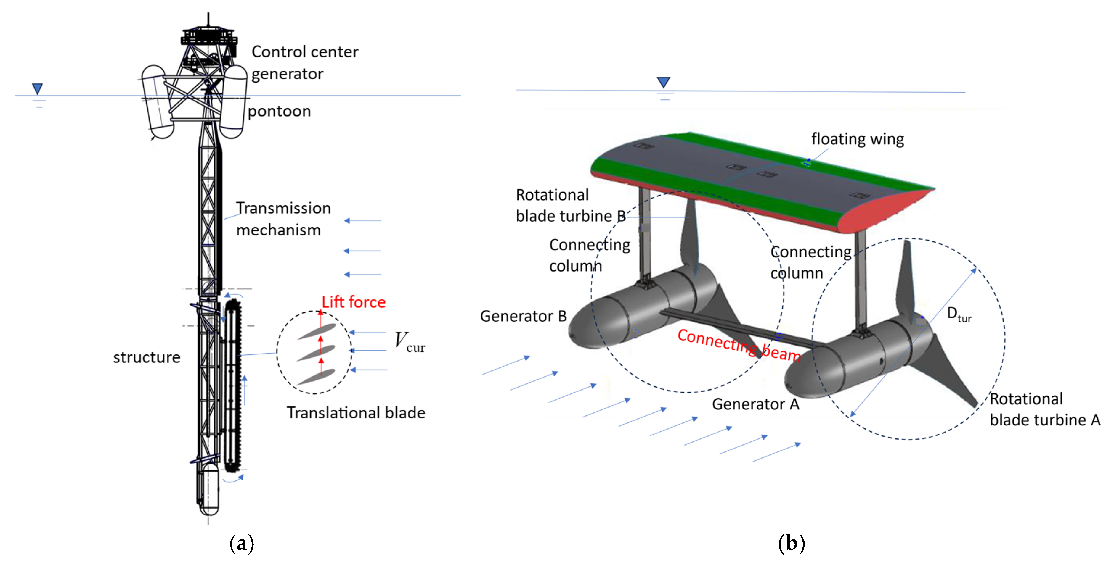
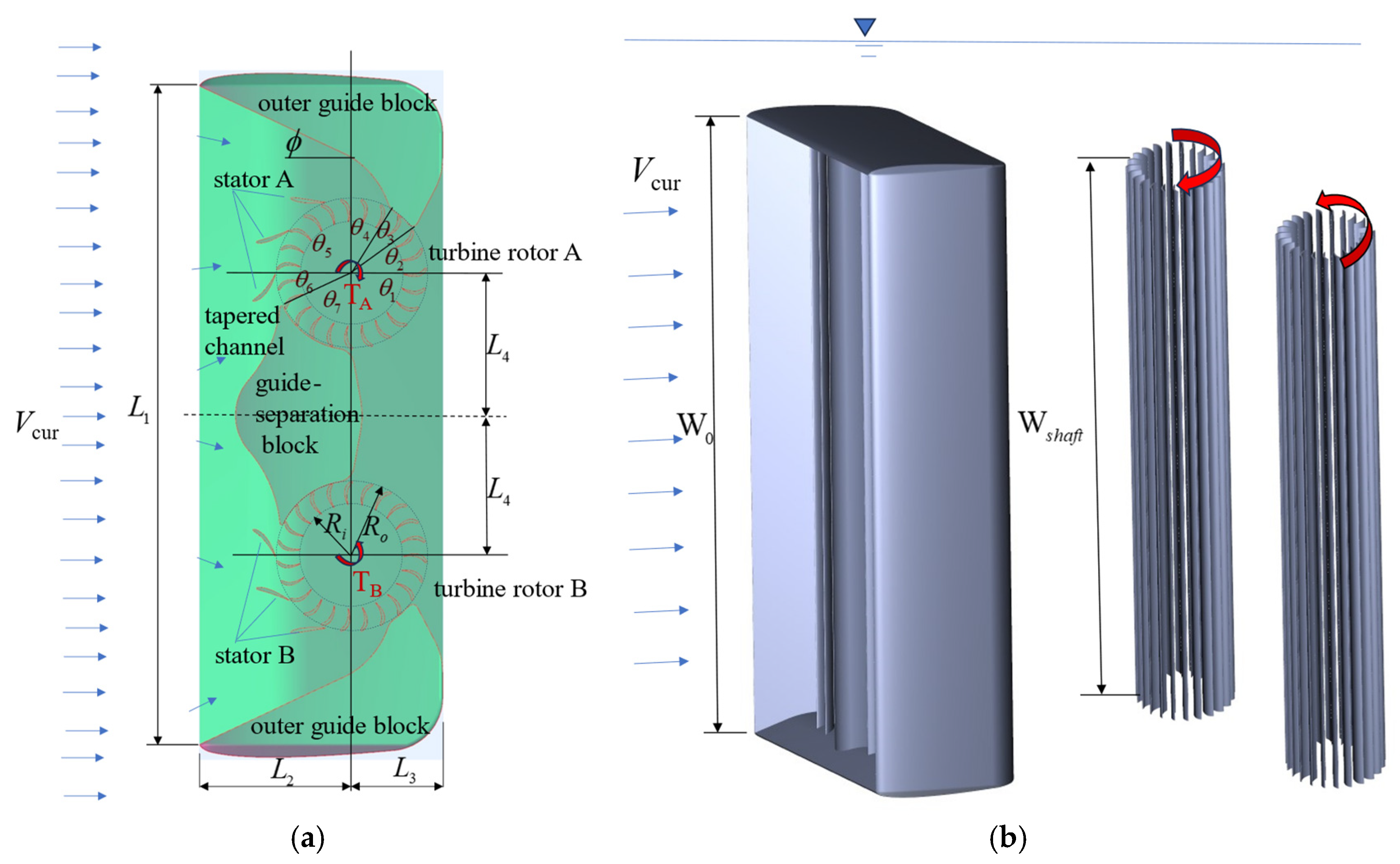
2.1. Configuration and Features of a Novel Ocean Current CFT Converter

As shown in Figure 2, two crossflow turbines, A and B, are integrated and set up in a tapered channel to guide the current into the two turbines. The two turbines rotate at the same speed but in opposite directions. When the two turbines are running under ocean currents, they generate torques T_A and T_B, respectively. Since they have the same specifications and rotate in different directions, the torque relation is T_A = −T_B. In other words, the torque summation is equal to zero; hence, the converter is self-stabilizing. For the horizontal-axis ocean turbine [2], the diameter of the turbine blade increases with power. The diameter of an MW-scale turbine is very large. Two turbines are connected by a beam. The distance between the two turbines needs to be very large to prevent interference between them. Therefore, the span of the connecting beam is very long, resulting in weak bending rigidity. This design requires two generators. In this study, the crossflow and vertical-axis ocean turbine is proposed. One can increase the power by using the same turbine diameter and increasing the length of the turbine axis; therefore, the center distance L₄ between the two turbines is very short, and the connecting structure is strong and safe. Because the distance between the centers of the two turbines of this novel converter is shorter than for the horizontal-axis converter, the power generated by the two turbines can be transmitted to a single generator using a transmission mechanism that also functions to transform the low rotating speed of the turbine to the high speed of the generator for high-efficiency electricity generation. To reduce the impact of typhoon waves, the ocean current power generator needs to dive to a safe depth, so the generator needs a high-pressure waterproof design. This proposed converter requires a single generator, so it can reduce waterproofing difficulties and costs.

The tapered channel is designed to increase the flow rate through the turbine. As shown in Figure 2, the tapered channel is composed of the outer guide blocks and a center guide-separation block. Therefore, the incident velocity V₁ is greater than the ocean current velocity V_cur, and the power and efficiency of the turbine increase effectively. A guide-separation block is installed between the two turbines to prevent the flow of water from the two turbines from interfering with each other and guides the ocean current to flow into the turbine along the turbine blades. Three guide vanes are positioned in front of the turbine inlet to guide the ocean current so that the water hits the rotor blades and pushes the turbine to rotate. The appropriate guide vane angle can produce an optimal water incident angle α₁, resulting in the best turbine performance.

The horizontal-axis energy converter is very wide horizontally and shallow vertically, making it unstable and prone to rolling. However, the outer geometry of this novel design is narrow horizontally and deep vertically. One can easily place the center of gravity at the bottom and the center of buoyancy at the top, giving it high stability.

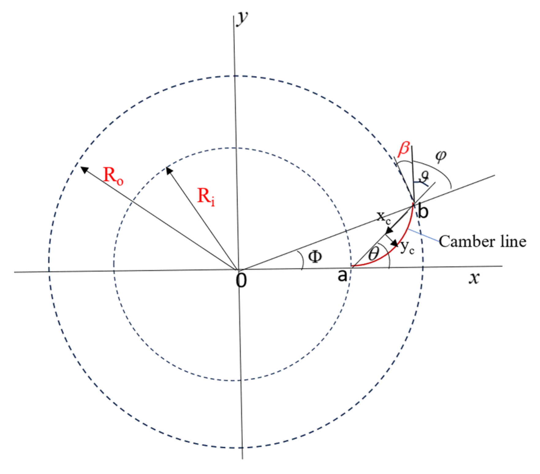
2.2. Configuration and Specifications of the Rotor Blades

In this study, the NACA profile of the blade is chosen [25]. The formula for the camber line is

$$y_c=\left\{\begin{array}{c}m{\displaystyle \frac{x_c}{p^2}}\left(2p-{\displaystyle \frac{x_c}{c}}\right),\hspace{1em}\hspace{1em}\hspace{1em}0\le x_c\le pc\\ m{\displaystyle \frac{c-x_c}{{\left(1-p\right)}^2}}\left(1+{\displaystyle \frac{x_c}{c}}-2p\right),\hspace{1em}pc\le x_c\le c\hspace{1em} \end{array}\right.$$

(1)

where m is the maximum camber, and p is the maximum camber position. One can derive the blade angle $\vartheta$ as

$$tan\vartheta ={\displaystyle \frac{d{y}_c\left(0\right)}{d{x}_c}}={\displaystyle \frac{2m}{p}}$$

(2)

As shown in Figure 3, the angle relation is

$$\theta =\left({\displaystyle \frac{\pi }{2}}-\beta \right)+\Phi -\vartheta$$

(3)

and

$$\tan \theta ={\displaystyle \frac{y_b-y_a}{x_b-x_a}}={\displaystyle \frac{R_o\sin \Phi }{R_o\cos \Phi -R_i}}$$

(4)

where $x_a=R_i, y_a=0; x_b=R_o\cos \Phi , y_b=R_o\sin \Phi$. Based on Equations (3) and (4), the relationship is obtained as

$${\displaystyle \frac{R_o\sin \Phi }{R_o\cos \Phi -R_i}}=\tan \left({\displaystyle \frac{\pi }{2}}-\beta +\Phi -\vartheta \right)$$

(5)

Given $\left\{\beta ,R_i,R_o,NACA m,p\right\}$ via Equation (5), and using the bisection method, the angle Φ is obtained. Furthermore, one can determine the chord of the blade as $c=\sqrt{{\left(x_b-x_a\right)}^2+{\left(y_b-y_a\right)}^2}$.

The thickness of the blade is

$$y_t=5tc\left[0.2969\sqrt{{\displaystyle \frac{x_c}{c}}}-0.1260\left({\displaystyle \frac{x_c}{c}}\right)-0.3516{\left({\displaystyle \frac{x_c}{c}}\right)}^2+0.2843{\left({\displaystyle \frac{x_c}{c}}\right)}^3-0.1015{\left({\displaystyle \frac{x_c}{c}}\right)}^4\right]$$

(6)

where t is the ratio of the maximum thickness to the chord.

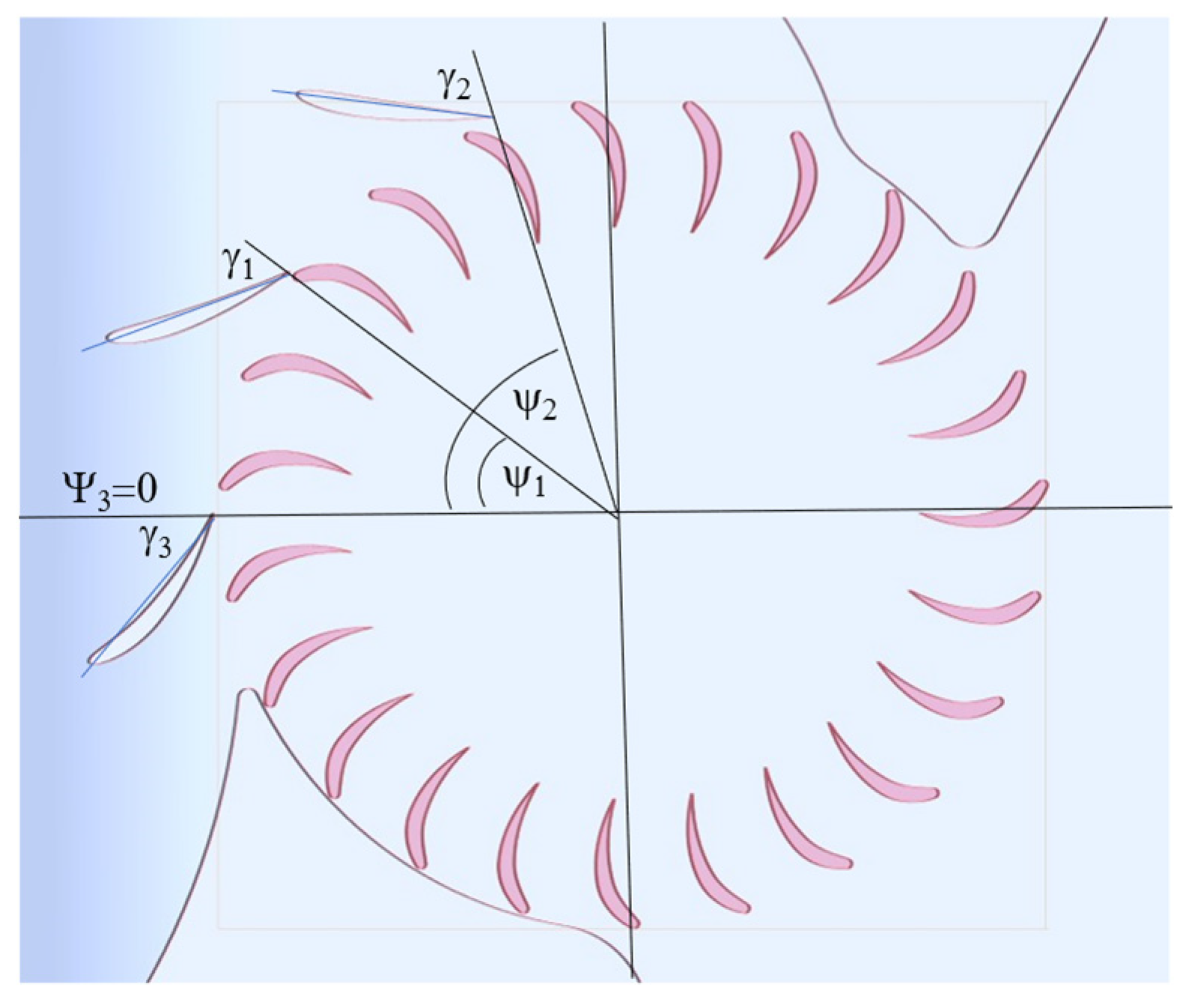
2.3. Configuration and Specifications of Guide Vanes

In this study, three guide vanes are set up as shown in Figure 4. The NACA profile of the vane is chosen. The formula of the camber line is as described in Equation (1). The relationship between the setting angles $\left\{{\psi }_i,{\gamma }_i\right\}$ and vane coefficients $\left\{m_i,p_i\right\}$ is

$$tan\left({\gamma }_i-{\psi }_i\right)={\displaystyle \frac{d{y}_c\left(0\right)}{dx}}={\displaystyle \frac{2m_i}{p_i}}$$

(7)

The thickness of the vane is as described in Equation (6).

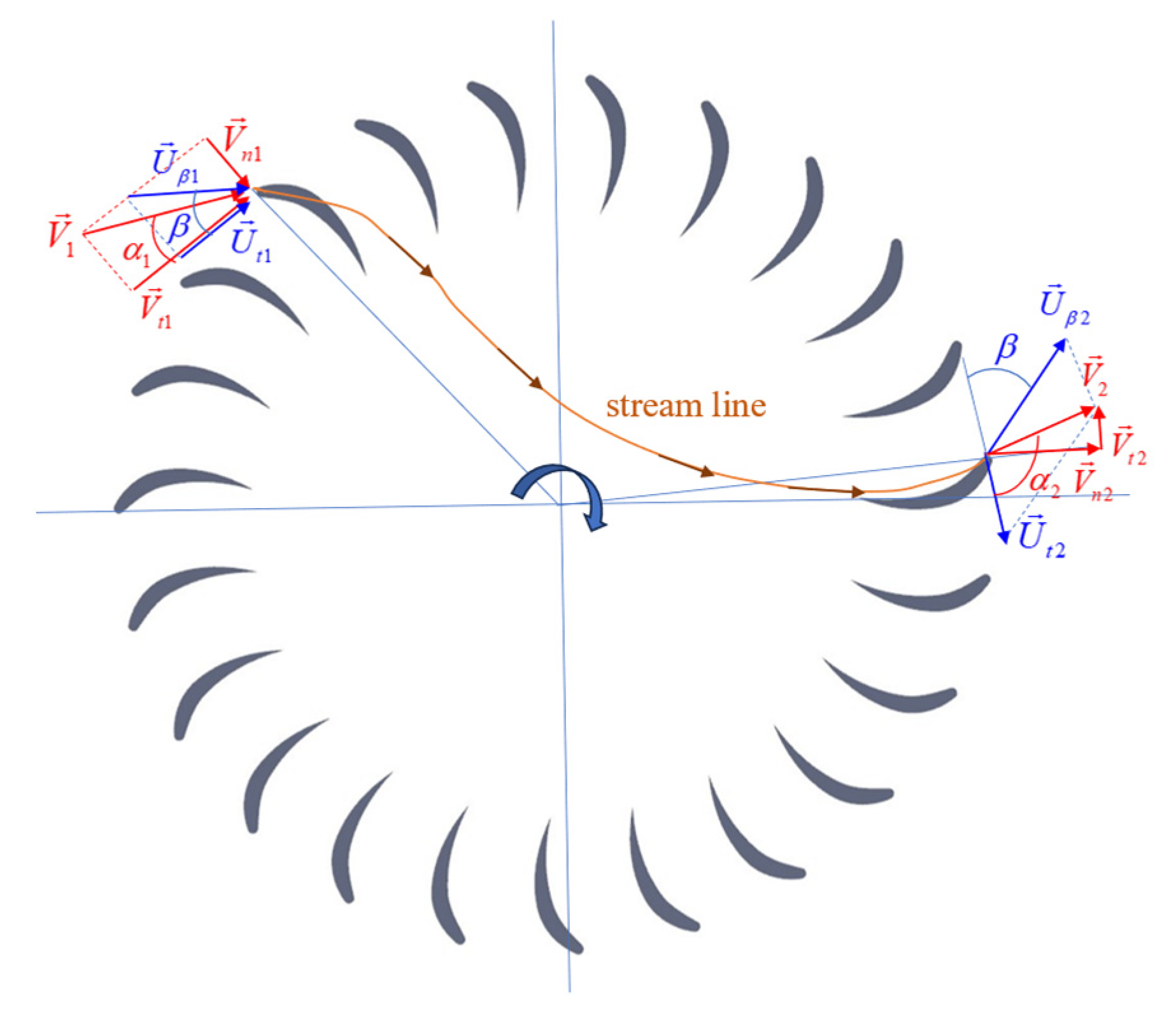
3. Theoretical Power and Efficiency of Ocean Current CFT Converters

As shown in Figure 5, the torque of a single turbine can be derived by using the Euler turbine equation

$$T_{tur}=\rho \left(Q/2\right)R_o\left(V_1\cos {\alpha }_1+V_2\cos {\alpha }_2\right)$$

(8)

where r is the fluid density, Q is the total flow rate of two turbines, R_o is the outer radius of the rotor, V₁ and α₁ are the incident velocity and angle at the inlet, respectively, and V₂ and α₂ are the departing velocity and angle at the outlet, respectively.

The total power of two turbines is given by

$$Powe{r}_{tur}=2T_{tur}\omega =\rho Q{R}_o\omega \left(V_1\cos {\alpha }_1+V_2\cos {\alpha }_2\right)$$

(9)

where the tangential velocity $U_{t1}=U_{t2}=R_o\omega \equiv U_t$. The velocity relationships at the turbine inlet and outlet are ${\overrightarrow{V}}_i={\overrightarrow{V}}_{ti}+{\overrightarrow{V}}_{ni}={\overrightarrow{U}}_{ti}+{\overrightarrow{U}}_{\beta i},i=1,2$. The normal velocity relationship at the inlet is

$$U_{\beta 1}\sin {\beta }_1=V_1\sin {\alpha }_1$$

(10)

where β₁ is the blade angle at the outlet. In fact, ${\beta }_1={\beta }_2\equiv \beta$. The tangential velocity relationship at the inlet is

$$U_{\beta 1}\cos {\beta }_1=V_1\cos {\alpha }_1-U_{t1}\mathrm{or} U_{\beta 1}={\displaystyle \frac{\left(V_1\cos {\alpha }_1-U_{t1}\right)}{\cos {\beta }_1}}$$

(11)

The relationship of the inlet–outlet relative velocities is expressed as

$$U_{\beta 2}=\delta U_{\beta 1}$$

(12)

where δ is the velocity coefficient depending on the turbine geometry and the operational conditions. Mockmore and Merryfield [16], Sinagra et al. [17], and Adanta et al. [19] assumed δ = 0.98 for the hydraulic crossflow turbine. In this study, the coefficient of velocity is derived based on continuity conditions as follows:

The relationship between the total flow rate Q₁ and incident velocity V₁ at the inlet is

$$Q_1=2V_1\sin {\alpha }_1{W}_{shaft}{R}_o{\theta }_{inlet}\mathrm{or} V_1=Q_1/2\sin {\alpha }_1{W}_{shaft}{R}_o{\theta }_{inlet}$$

(13)

where ${\theta }_{inlet}$ is the inlet angle, and W_shaft is the length of the turbine shaft. The total flow rate Q₂ at the outlet is

$$Q_2=2W_{shaft}{R}_o{\theta }_{outlet}{V}_{n2}$$

(14)

where the normal velocity at the outlet $V_{n2}=U_{\beta 2}\sin \beta$. ${\theta }_{outlet}$ is the outlet angle. Substituting Equation (12) into Equation (14), one obtains

$$Q_2=2W_{shaft}{R}_o{\theta }_{outlet}\delta U_{\beta 1}\sin \beta$$

(15)

Based on the continuity condition, Q₁ = Q₂ $\equiv$ Q, and Equation (11), the velocity coefficient is obtained as follows:

$$\delta =r_{\theta }{\displaystyle \frac{\sin {\alpha }_1}{\left(\cos {\alpha }_1-r_{ts}\right)}}\cot \beta$$

(16)

where the tip speed ratio $r_{ts}=U_t/V_1$. The ratio of the inlet–outlet area $r_{\theta }={\theta }_{inlet}/{\theta }_{outlet}$.

The velocity relationships at the outlet are defined as

$$V_2\cos {\alpha }_2=U_{\beta 2}\cos \beta -U_t=\delta \left(V_1\cos {\alpha }_1-U_t\right)-U_t$$

(17)

$$V_2\sin {\alpha }_2=\delta U_{\beta 1}\sin \beta =V_1\sin {\alpha }_1{r}_{\theta }$$

(18)

Based on Equations (17) and (18), the departing velocity at the outlet is

$$V_2=V_1\sqrt{{\left(r_{\theta }\sin {\alpha }_1\right)}^2+{\left(r_{\theta }\sin {\alpha }_1\cot \beta -r_{ts}\right)}^2}$$

(19)

Substituting Equations (16) and (17) into Equation (9), the power is

$$Powe{r}_{tur}=\rho Q{V}_1^2{r}_{ts}\left(\cos {\alpha }_1-r_{ts}\right)\left(1+r_{\theta }{\displaystyle \frac{\sin {\alpha }_1}{\left(\cos {\alpha }_1-r_{ts}\right)}}\cot \beta \right)$$

(20)

This equation describes the effects of the density r, the flow rate Q, the incident angle α₁, the tip speed ratio $r_{ts}=U_t/V_1$, the blade angle β, and the inlet–outlet area ratio $r_{\theta }$ on the power of the turbine. It is a modified formula that differs from the traditional one proposed by Mockmore and Merryfield [16] for the hydraulic CFT, $powe{r}_{tur}=\rho Q{V}_1^2{r}_{ts}\left(\cos {\alpha }_1-r_{ts}\right)\left(1+\delta \right)$, which excludes the effects of the blade angle β and the inlet–outlet area ratio $r_{\theta }$.

Based on the conservation of energy, the energy relationship is expressed as

$$Powe{r}_{inlet}=Powe{r}_{tur}+Powe{r}_{outlet}$$

(21)

where power_inlet is the total power entering the turbines, power_tur is the output power of the turbine from the fluid energy to the mechanical energy, and Power_outlet is the flow-out power from the turbine outlet. Ocean currents do not have potential energy. The pressure difference between the inlet and outlet is small; therefore, the fluid energy at the outlet is kinetic only. Thus, $Powe{r}_{outlet}={\displaystyle \frac{1}{2}}\rho Q{V}_2^2$. Furthermore, the efficiency of the converter is

$$\eta ={\displaystyle \frac{Powe{r}_{tur}}{Powe{r}_{inlet}}}={\displaystyle \frac{1}{1+\xi r_V^2}}$$

(22)

where $\xi ={\displaystyle \frac{1}{2r_{ts}\left(\cos {\alpha }_1+r_{\theta }\sin {\alpha }_1\cot \beta -r_{ts}\right)}}$, $r_V=\sqrt{{\left(r_{\theta }\sin {\alpha }_1\right)}^2+{\left(r_{\theta }\sin {\alpha }_1\cot \beta -r_{ts}\right)}^2}$.

Assuming the parameters $\left\{{\alpha }_1,r_{\theta },r_{ts},Q\right\}$ are independent, the optimal efficiency can be obtained by adjusting the tip speed ratio r_ts. In other words, one can determine the optimal rotating speed N for the highest efficiency. Letting $d\eta /d{r}_{ts}=0$, one obtains

$$\begin{array}{l}\left[\left(\cos {\alpha }_1+r_{\theta }\sin {\alpha }_1\cot \beta \right)-2r_{ts}\right]\left[{\left(r_{\theta }\sin {\alpha }_1\right)}^2+{\left(r_{\theta }\sin {\alpha }_1\cot \beta -r_{ts}\right)}^2\right]\\ \hspace{1em}\hspace{1em}\hspace{1em}\hspace{1em}\hspace{1em}+2\left[r_{ts}\left(\cos {\alpha }_1+r_{\theta }\sin {\alpha }_1\cot \beta \right)-r_{ts}^2\right]\left(r_{\theta }\sin {\alpha }_1\cot \beta -r_{ts}\right)=0\end{array}$$

(23)

By using the bisection method and applying Equation (23), the optimal tip speed ratio r_ts,opt can be determined. Substituting it back into Equation (22) gives the optimal efficiency.

4. Numerical Results and Discussion

4.1. Power Comparison Using Empirical Formula and the CFD Method

As illustrated in Figure 6, the CFD modeling procedure consists of the following steps:

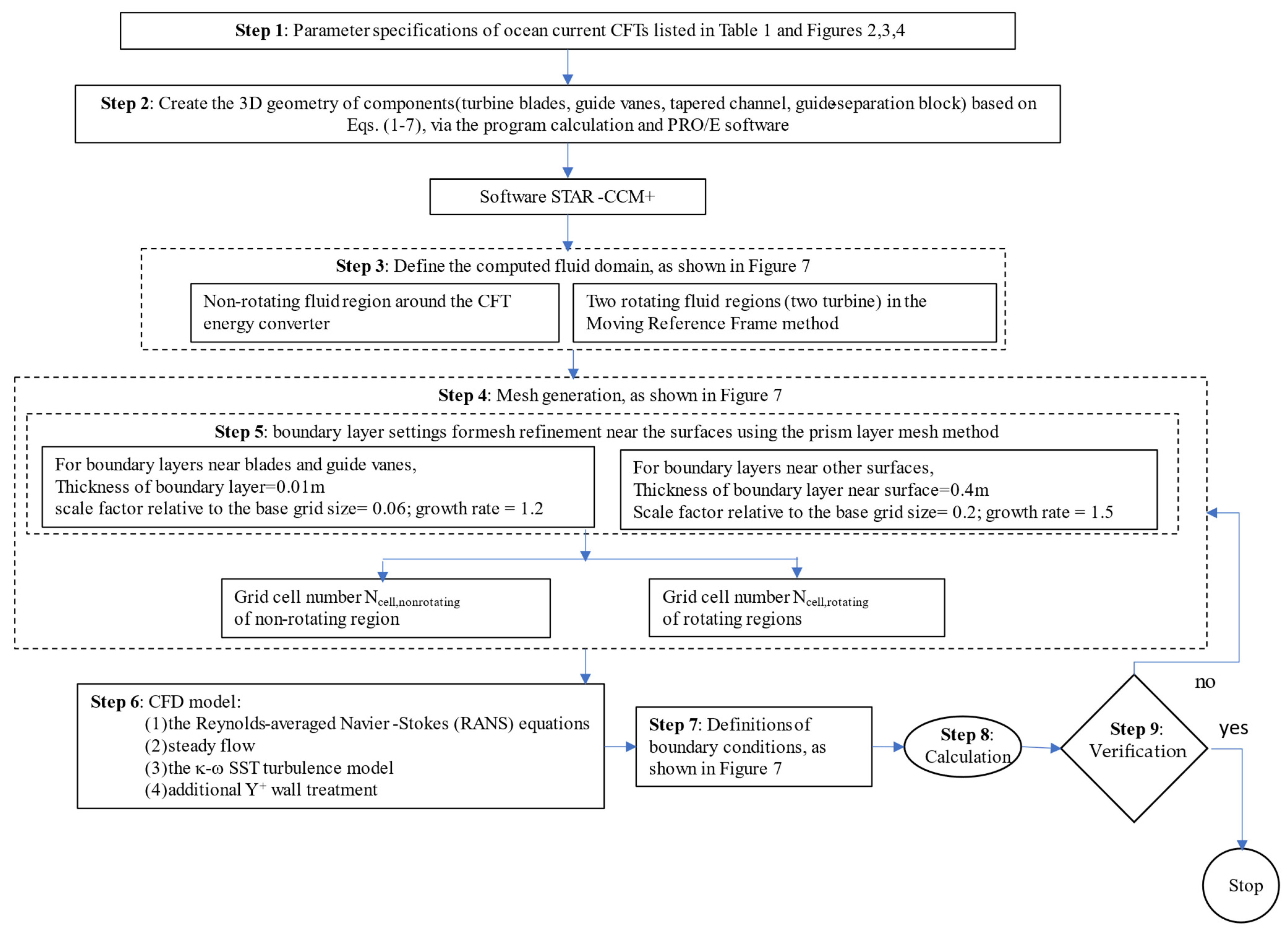
• Step 1: Specification of Parameters

The parameters of CFD model are classified as four kinds: (1) channel parameters, as shown in Figure 2; (2) rotor parameters, as shown in Figure 3; (3) guide vane parameters, as shown in Figure 4; and (4) operating parameters. These specifications are listed in

Table 1. Parameter specifications.

Classification	Parameter	Dimension
Structure of channel	Channel horizontal width L1	37.02 m
	Distance from turbine center to channel inlet L2	8.20 m
	Distance from turbine center to channel outlet L3	5.09 m
	Distance between two turbine centers L4	-
	Channel vertical length W0	54.213 m
Turbine rotor	Outer radius of rotor Ro	4.20 m
	Inner radius of rotor Ri	2.887 m
	length of turbine shaft Wshaft	50.0 m
	Maximum thickness of blade m	0.2
	Maximum camber position of blade p	0.4
	Blade angle β	45°
	Number of rotor blades Nblade	23
Guide vane	Directions of three vanes ψ1/ψ2/ψ3	35°/70°/0°
	Setting angle of three vanes γ1/γ2/γ3	78°/88°/73°
	chords of three vanes c1/c2/c3	1.9688 m
	Maximum thickness of three vanes m1/m2/m3	0.05/0.03/0.1
	Maximum camber position of three vanes p1/p2/p3	0.4
Operating parameter	Angle of turbine inlet θinlet	136.5°
	Angle of turbine outlet θoutlet	90°
	Ratio of inlet–outlet area $r_{\theta }={\theta }_{inlet}/{\theta }_{outlet}$	1.517
	Current velocity Vcur	1.6 m/s
	Rotating speed N	2.4 rpm

.

• Step 2: Construction of 3D Component Geometries

Using Equations (1)–(7), the 3D coordinates of curved surfaces for the turbine blades and guide vanes can be determined through numerical calculations. Moreover, those for the tapered channel and the guide-separation block can be easily determined. These coordinates are then utilized to construct the 3D geometries in PTC Creo 10.0.2.0 CAD software, as shown in Figure 2.

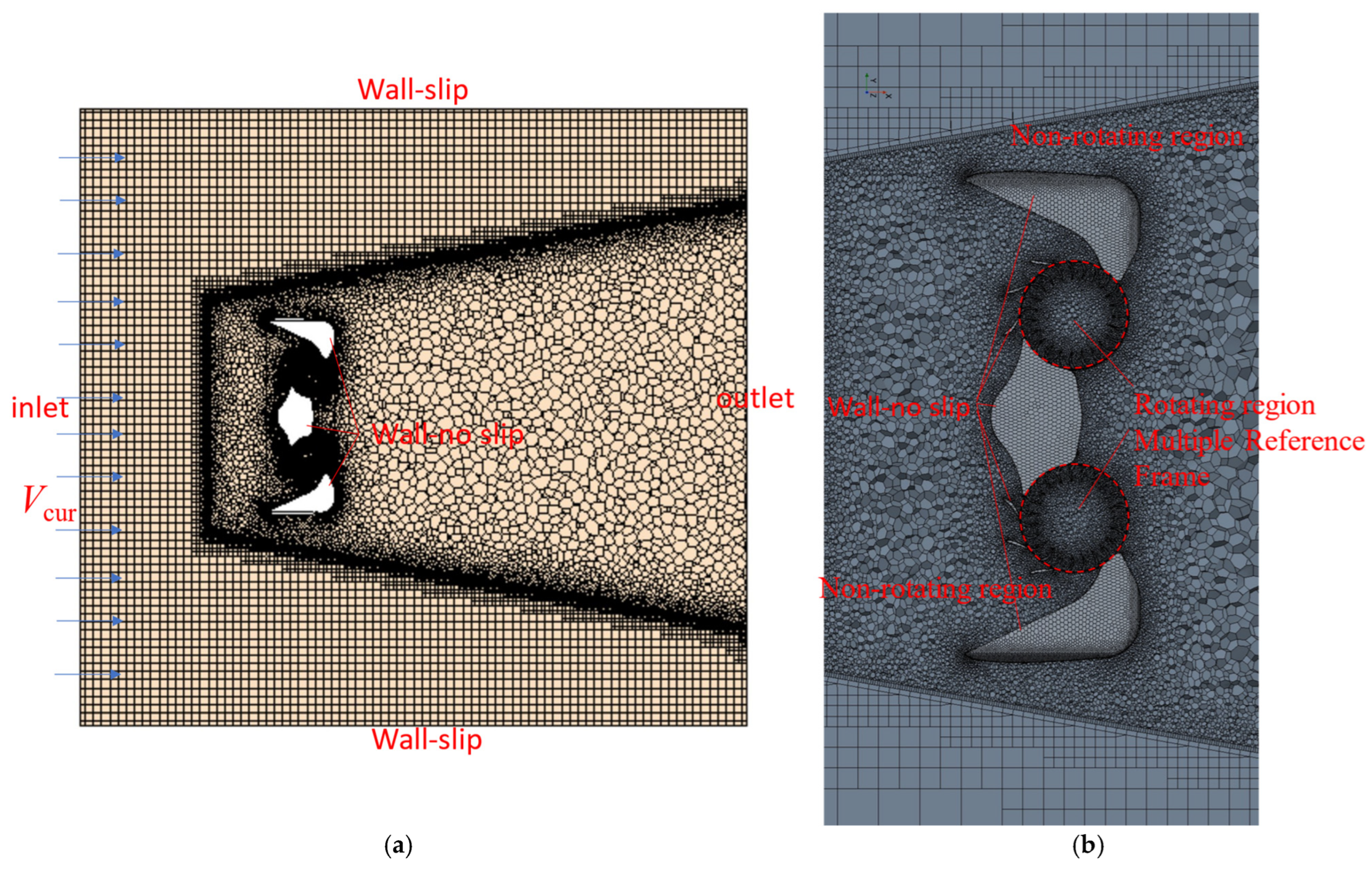
• Step 3: Creation of the CFD Fluid Domain

The geometric models are imported into the STAR-CCM+ 2021.1 CFD software, where they are segmented into respective parts. The computational domain comprises two rotating regions for the turbine rotors and one stationary region representing the supporting structure, as shown in Figure 7.

• Step 4: Mesh Generation of the Fluid Domain

The domain is discretized to form a computational mesh suitable for numerical simulation, as shown in Figure 7. N_{cell,nonrotating} is the grid cell number of the nonrotating region. N_{cell,rotating} is the grid cell number of the rotating region.

• Step 5: Boundary Layer Mesh Settings

To accurately resolve near-wall flow features, prism-layer mesh refinement is applied along all solid surfaces, as shown in Figure 7b. The settings are as follows:

• Near blades and guide vanes:

  ○

  Boundary layer thickness: 0.01 m;

  ○

  Scale factor (relative to base mesh): 0.06;

  ○

  Growth rate: 1.2.

• Near other surfaces:

  ○

  Boundary layer thickness: 0.4 m;

  ○

  Scale factor (relative to base mesh): 0.2;

  ○

  Growth rate: 1.5.

These mesh settings are critical for achieving reliable boundary layer resolution and ensuring the accuracy of the CFD predictions.

• Step 6: CFD Model Setup

The computational model is based on the following:

• Reynolds-Averaged Navier–Stokes (RANS) equations;
• Steady-state flow assumption;
• k-ω SST turbulence model;
• Additional y+ based wall treatment for near-wall modeling.

• Step 7: Definition of Boundary Conditions

Boundary conditions applied to the computational domain are detailed in Figure 7.

• Step 8: Numerical Simulation

The CFD solver is executed under the prescribed conditions to compute the flow field and turbine performance.

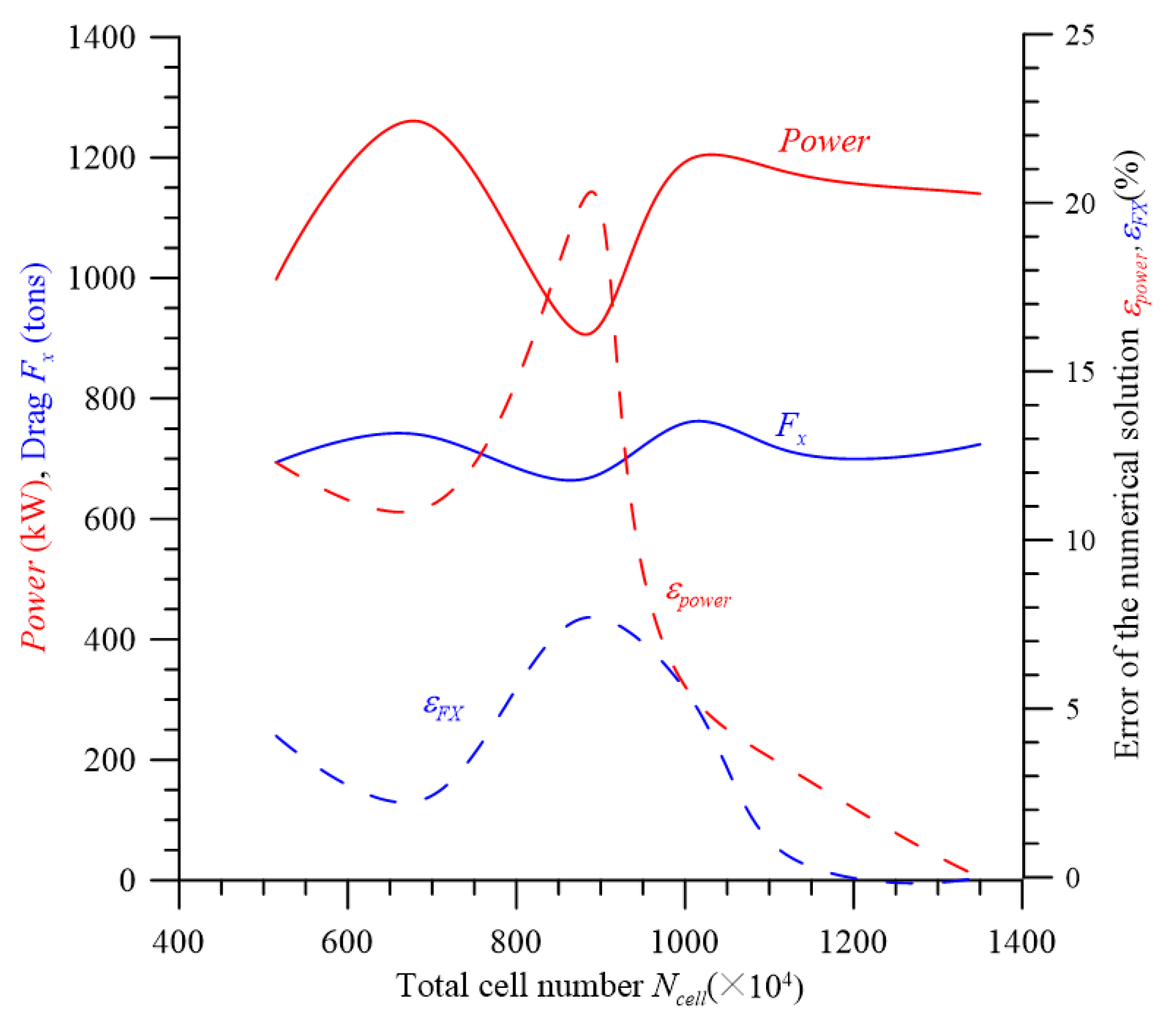
• Step 9: Grid Independence Verification

A mesh sensitivity study is conducted, and results are presented later to ensure that the solution is independent of the mesh resolution.

First, a comparison of the numerical results using the CFD method and the empirical formula in Section 3 is carried out as follows:

All the parameters for the converter are listed in Table 1.

Table 2. Comparison of theoretical and CFD results.

L4 (m)	Flow Rate Q (m3/s) (*)	Average Incident Angle α1 (deg) (*)	Tip Speed Ratio rts = Ut/V1 (#)	Average Incident Velocity V1 (m/s) (**)	Power (kW) (CFD) (*)	Power (kW) (***)	Error of Power (%)
5.0	629.37	32.8	0.909	1.161	594.6	595.4	0.13
6.0	689.56	34.0	0.857	1.232	744.6	754.5	1.33
6.5	698.05	33.4	0.833	1.267	799.0	801.0	0.25
7.0	706.44	30.8	0.766	1.379	914.0	916.9	0.32
8.0	707.90	25.7	0.647	1.631	1133.7	1139.3	0.49
9.0	714.05	23.5	0.590	1.790	1307.5	1288.6	1.45
13.0	754.73	20.0	0.491	2.148	1640.2	1652.7	0.76

*: by CFD method; **: by substituting the parameters {Q, R_o, W_shaft, α₁, θ_inlet } into Equation (13); #: by substituting V1 into r_ts = U_t/V₁; ***: by substituting the parameters {Q, α₁, β, r_ts, r_θ, V₁} into Equation (20).

shows the effect of the turbine center distance L₄ on the incident angle α₁, the incident velocity V₁, the tip speed ratio r_ts, and two powers determined using the empirical formula and the CFD method. Using the CFD method, one can obtain the flow rate Q, power, incident angle α₁, and 3D velocity field, force, moments, etc.

Grid independence verification was conducted, and the results are presented in

Table 3. Grid independent verification.

Grid Type	Grid	Ncell,rotating/ Ncell,nonrotating	$\dot{\mathit{m}}$(kg/s)	εm (%) *	Power (kw)	εpower (%) *	Fx (N)	εFX (%) *
A	coarse	6,802,362/ 8,516,028	654,652	1.34	1065.92	13.65	6,654,329	0.10
B	medium	10,809,792/ 13,204,668	656,401	1.08	1190.20	3.59	6,759,912	1.48
C	fine	12,788,736/ 15,806,913	663,557	0	1234.47	0	6,661,119	0

*: Equation (24).

. All converter parameters are detailed in Table 1, with the exception of the following values: L₂ = 8.56 m, L₃ = 4.66 m, L₄ = 8.0 m, W_shaft = 48 m, W₀ = 52.21 m, N_blade = 31, and β = 44°. The influence of different grid types on flow rate, power output, and drag force was evaluated, with corresponding results summarized in Table 3. The numerical solution error, denoted as ε, was computed for each grid configuration according to the method described in [26].

$${\epsilon }_m=\left|{\displaystyle \frac{{\dot{m}}_i-{\dot{m}}_C}{{\dot{m}}_C}}\right|\times 100\%, {\epsilon }_{power}=\left|{\displaystyle \frac{powe{r}_i-powe{r}_C}{powe{r}_C}}\right|\times 100\%, {\epsilon }_{FX}=\left|{\displaystyle \frac{F_{Xi}-F_{XC}}{F_{XC}}}\right|\times 100\%,i=A,B,C$$

(24)

The analysis reveals that increasing the number of grid cells results in a reduction in numerical error.

Furthermore, Figure 8 provides a visual representation of the grid independence study, based on the converter configuration listed in Table 1, with modified parameters: L₂ = 8.47 m, L₃ = 5.09 m, L₄ = 7.875 m, W_shaft = 51.5 m, W₀ = 55.63 m, N_blade = 23, β = 34°, and γ₁/γ₂/γ₃ = 55°/63°/50°. The impact of the total number of cells, N_cell,total (=N_{cell,rotating} + N_{cell,nonrotating}), on power output, drag force, and numerical error is illustrated in Figure 8. It was observed that when N_cell,total < $1.2 \times {10}^7$, both power and drag force exhibit significant sensitivity to changes in cell count. Conversely, for N_cell,total > $1.2 \times {10}^7$, the numerical error decreases markedly with increasing cell count.

Figure 9a shows the local flow field of the center distance L₄ = 8 m using the CFD method. It is found that the incident angle α₁~25.7°, the inlet angle θ_inlet = 136.5°, and the outlet angle θ_outlet~90°, as listed in Table 2. Due to the complexity of 3D velocity distribution, it is challenging to accurately calculate the average incident velocity V₁ based on the velocity field using CFD. Fortunately, the average incident velocity can be obtained using Formula (13) based on the continuity condition. Further, by substituting the parameters {Q, α₁, β, r_ts, r_θ, V₁} into the empirical Formula (20), the theoretical power can be obtained. Table 2 shows that the powers obtained using the CFD method and empirical Formula (20) are very similar.

The flow fields with different values of center distance L₄ are shown in Figure 9. As shown in Figure 9b, where L₄ = 5 m, because the distance between the two turbines is too short, the streams from the outlet of the two turbines flow toward the rear and middle and mix together, resulting in significant interference with each other. The maximum flow speed in the flow field is 2.96 m/s. Figure 9c, with L₄ = 6.5 m, shows that the water at the outlet of the two turbines flows horizontally toward the rear, causing no interference between the two. The maximum flow velocity is 3.13 m/s. If the distance L₄ is further increased to 8.0 m, as shown in Figure 9a,d, the outlet water flows horizontally to the rear and outside without interference. The maximum flow velocity is 3.44 m/s. If the distance L₄ = 13.0 m, as shown in Figure 9e, the water from the two outlets flows horizontally to the rear and outside without interference. The maximum flow velocity is 3.85 m/s.

Table 2 shows that the larger the turbine center distance L₄ is, the larger the flow rate Q and the power are. The powers obtained using the CFD method and empirical Formula (20) are very similar.

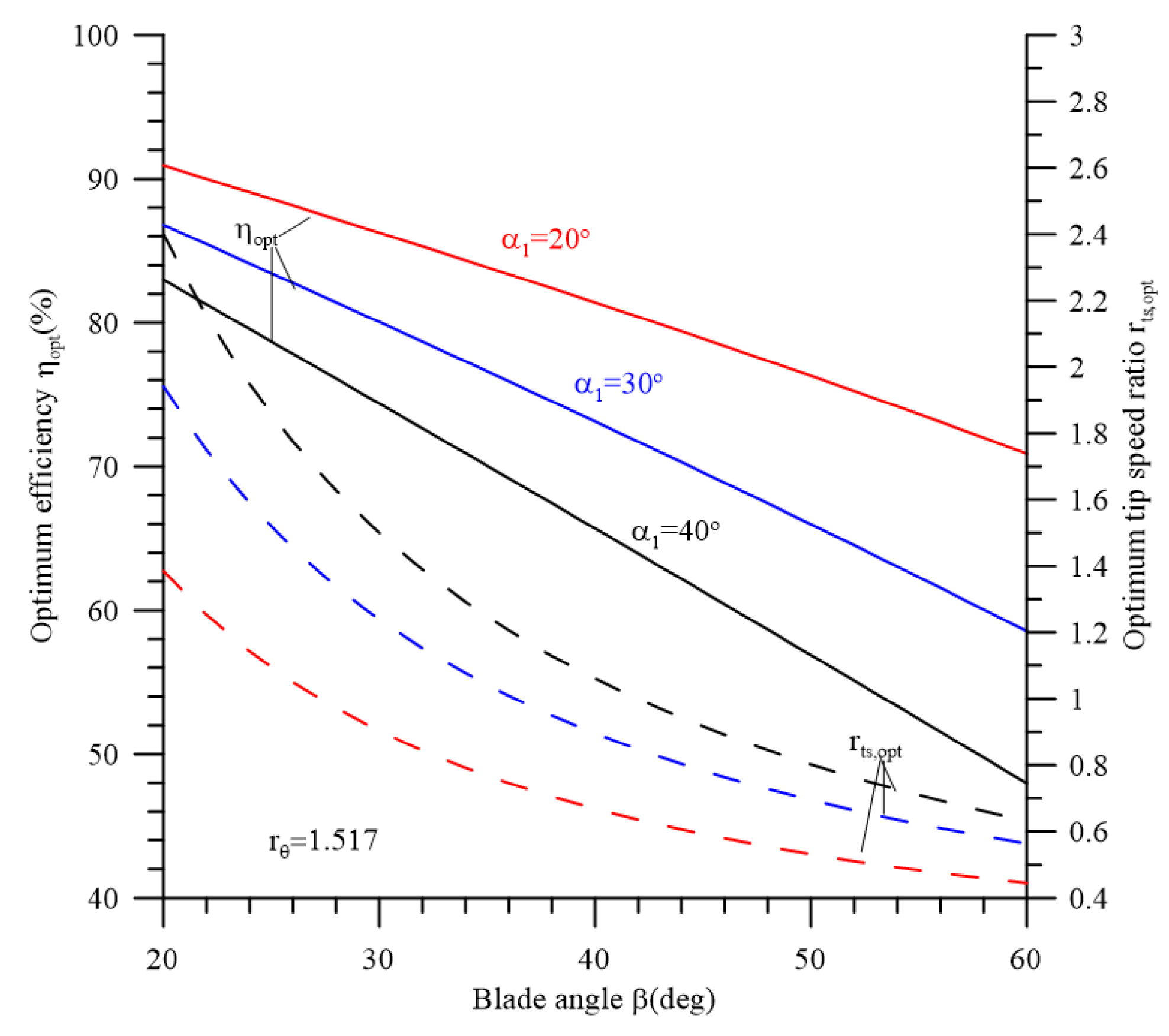
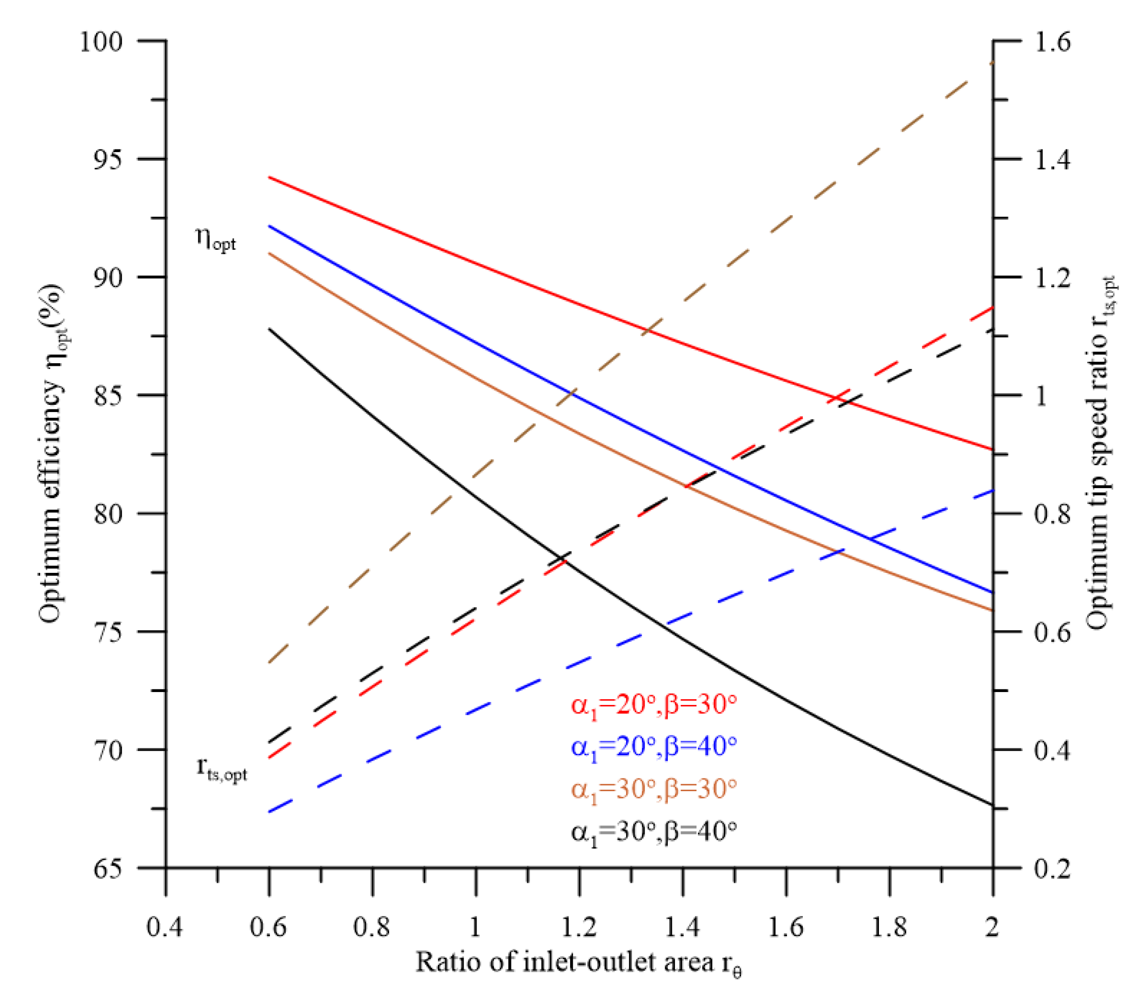
4.2. Theoretical Performance Using the Empirical Formula

Figure 10 demonstrates the effect of the tip speed ratio r_ts = U_t/V₁ on the performance of the turbine. The parameters of this case are the same as those in Table 1, except for the rotating speed N. Using Equations (20) and (22), the association of the tip speed ratio r_ts and the turbine center distance L₄ with the power and efficiency η is determined and shown in Figure 10a,b. It is observed in Figure 10a that for turbine center distance L₄ = 13 m, the mass flow rate $\dot{m} = 7.536 \times {10}^5 (\mathrm{kg}/\mathrm{s})$, and the incident angle α₁ = 21.5°, and based on Equations (20) and (22), if the tip speed ratio r_ts is increased above 0.1, the power and efficiency η are significantly increased. The maximum power = 1673 kW and optimum efficiency η_opt = 77.38% at r_ts =0.60. Using the CFD method, for r_ts = 0.548 and L₄ = 13 m, the corresponding power is 1640 kW. The errors for the two powers are about 2%. If the tip speed ratio r_ts is increased from the critical point, the power and efficiency η are significantly decreased. Moreover, for turbine center distance L₄ = 15 m, the mass flow rate $\dot{m} = 7.736 \times {10}^5 (\mathrm{kg}/\mathrm{s})$ and the incident angle α₁ = 20.0°, and based on Equations (20) and (22), the maximum power is 2065 kW and optimum efficiency η_opt = 78.98% at r_ts = 0.59. Using the CFD method, for r_ts = 0.478 and L₄ = 15 m, the corresponding power is 2070 kW. The power error Is about 0.2%.

It is observed in Figure 10b that for turbine center distance L₄ = 8 m, the mass flow rate $\dot{m} = 7.256 \times {10}^5 (\mathrm{kg}/\mathrm{s})$ and the incident angle α₁ = 26.5°, and based on Equations (20), (22) and (24), the maximum power is 1137.8 kW and the optimal efficiency η_opt = 72.69% at r_ts = 0.700. Using the CFD method, for r_ts = 0.661 and L₄ = 8 m, the corresponding power is 1133.7 kW. The error of the two powers is about 0.36%. Moreover, for turbine center distance L₄ = 6 m, the mass flow rate $\dot{m} = 7.068 \times {10}^5 (\mathrm{kg}/\mathrm{s})$ and the incident angle α₁ = 34.3°, and based on Equations (20) and (22), the maximum power is 754.8 kW and the optimum efficiency η_opt = 65.91% at r_ts = 0.85. Using the CFD method, for r_ts = 0.892 and L₄ = 6 m, the corresponding power is 744.6 kW. The error of the two powers is about 1.4%.

The effects of the incident angle α₁, the turbine blade angle β, and the ratio of inlet–outlet area $r_{\theta } = {\theta }_{inlet}/{\theta }_{outlet}$ on the optimal efficiency η_opt and optimal tip speed ratio r_ts,opt are investigated according to Equations (22) and (23), and the results are shown in Figure 10, Figure 11 and Figure 12. The optimal efficiency η_opt and optimal tip speed ratio r_ts,opt are obtained via the empirical Formulas (22) and (23) using three assumptions: (1) tip speed ratio r_ts is independent of the flow rate Q and the incident angle α₁, (2) the number of rotor blades is infinite, and (3) any blade angle β is allowed.

As shown in Figure 11 and Figure 12 and based on the empirical Formulas (22) and (23), the smaller the incident angle α₁ and the turbine blade angle β, the higher the optimal efficiency η_opt. If the turbine blade angle β is very small, the flow channel becomes narrow, resulting in a lower flow rate Q. On the other hand, the larger the setting angles γ_i of the guide vanes, the smaller the incident angle α₁, as shown in Figure 4. However, if the setting angle γ_i is very large, the flow resistance increases, resulting in a lower flow rate Q. The smaller the incident angle α₁, the lower the optimal tip speed ratio r_ts,opt. The smaller the turbine blade angle β, the higher the optimal tip speed ratio r_ts,opt. As shown in Figure 13, the smaller the ratio of the inlet–outlet area $r_{\theta }$, the higher the optimal efficiency η_opt. The smaller the ratio of inlet–outlet area $r_{\theta }$, the lower the optimal tip speed ratio r_ts,opt.

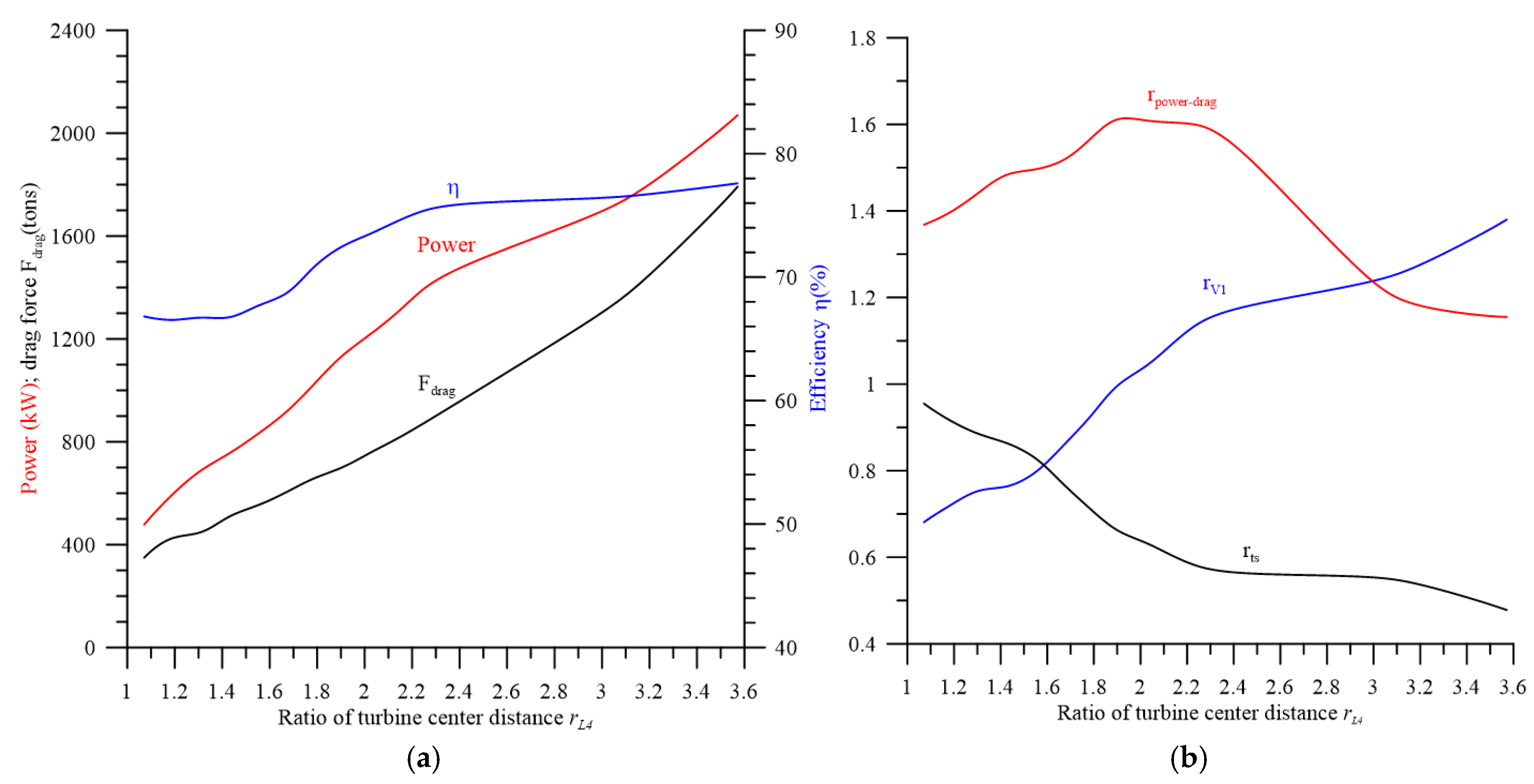
4.3. Determining the Effect of the Turbine Center Distance Ratio on Energy Converter Performance Using CFD

The effect of the turbine center distance ratio r_L4 = L₄/R_o on the performance of the energy converter is investigated using the CFD method; the results are shown in Figure 14a,b. All the parameters are the same as those listed in Table 1. As shown in Figure 14a, the longer the ratio r_L4, the larger the flow rate Q, the power, and the drag force F_drag. When the ratio r_L4 < 1.50, the efficiency η is approximately 66.8% and low. This is because the distance between the two turbines is too short and interference of the flow of the two turbines occurs at the outlet, as shown in Figure 9b. The efficiency η is significantly increased when the turbine center distance ratio r_L4 is increased above 1.50. For example, when r_L4 = 2.50, the optimal efficiency η_opt = 76.0%. Furthermore, the efficiency η is also slightly increased when the turbine center distance ratio is increased above r_L4 = 2.50.

As shown in Figure 14b, the larger the turbine center distance ratio r_L4 is, the larger the incident velocity V₁ and the incident velocity ratio $r_{V1}=V_1/V_{cur}$ are. The power increases with the turbine center distance ratio r_L4. If r_L4 < 1.90, the incident velocity V₁ is lower than the current velocity V_cur, i.e., the incident velocity ratio $r_{V1} = V_1/V_{cur}<1$. If r_L4 = 1.90, the incident velocity V₁ is equal to the current velocity V_cur, i.e., the incident velocity ratio $r_{V1} = V_1/V_{cur}=1$. The power–drag ratio r_power-drag is maximum when r_L4 = 1.90. This is beneficial for the mooring design of ocean current power generation.

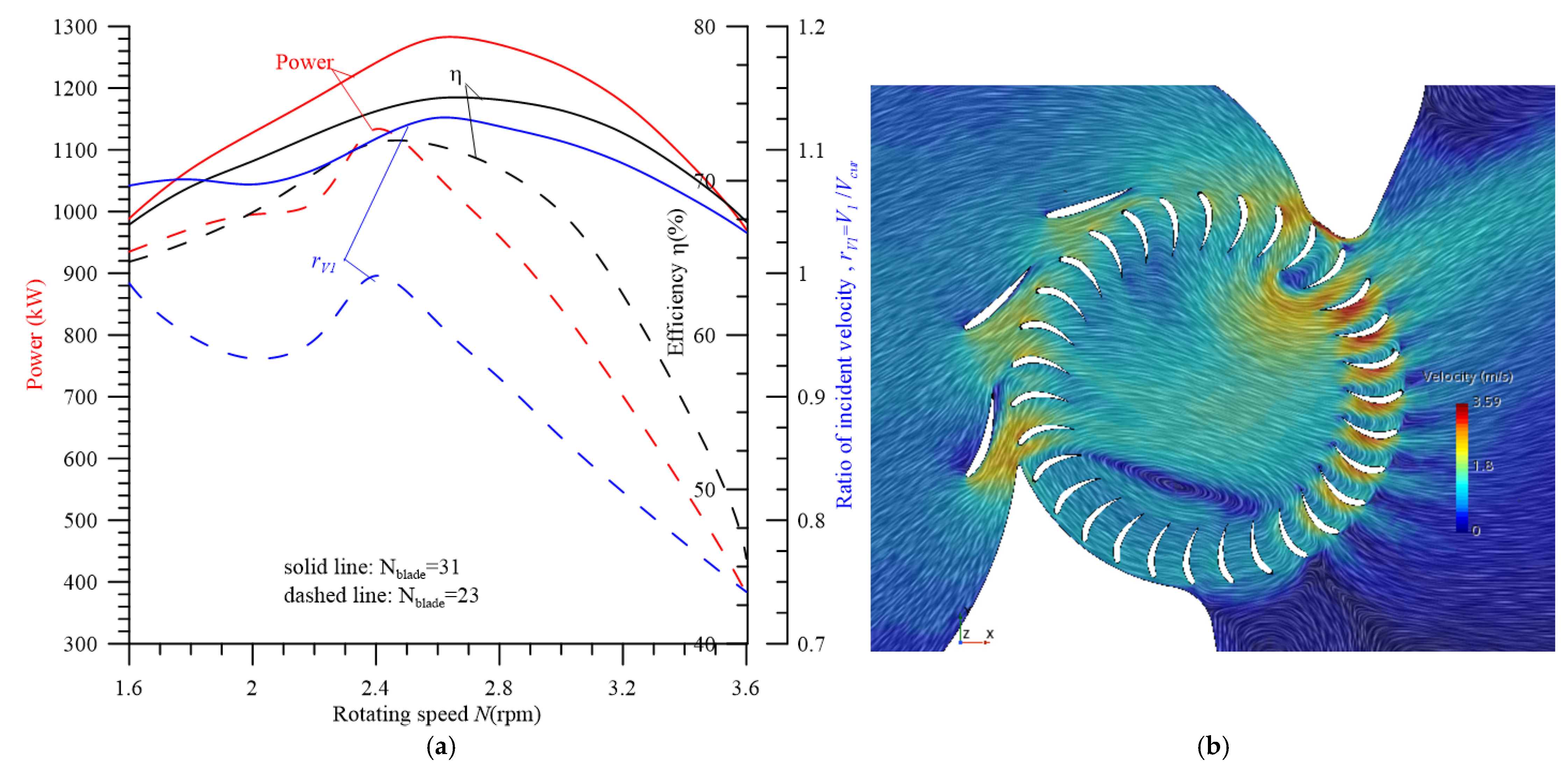
4.4. Determination of the Effect of Rotating Speed and Blade Number on Turbine Performance Using CFD

Figure 15a demonstrates the effect of the rotating speed N and the number of rotor blades N_blade on the performance of the turbine when the number of rotor blades N_blade = 23 and 31. All the parameters are the same as those in Table 1, except for the rotating speed N. For the case where N_blade = 23, it is found that for 2.0 rpm < N < 2.2 rpm, the power and the incident velocity ratio r_V1 = V₁/V_cur slightly increase with the rotating speed N. For 2.2 rpm < N < 2.4 rpm, the power and the incident velocity ratio r_V1 increase significantly with the rotating speed N. When N = 2.4 rpm, the power is at its maximum, power_max = 1133.7 kW, the incident velocity ratio r_V1 = 1.619, and the maximum efficiency η_max = 72.48%. When N > 2.4 rpm, the power, the incident velocity ratio r_V1, and the efficiency η decrease significantly with the rotating speed N.

For the case where N_blade = 31, it is found that if N = 2.6 rpm, the maximum power is 1281.6 kW, the incident velocity ratio r_V1= 1.762, and the maximum efficiency η_max = 75.35%. These results are obviously better than those for the case where N_blade = 23. Furthermore, Figure 15b shows the local flow fields with L₄ = 8 m, N_blade = 31, and N = 2.6 rpm. Comparing Figure 15b, where N_blade = 31, with Figure 9d, where N_blade = 23, shows that the flow field with N_blade = 31 is smoother than that with N_blade = 23.

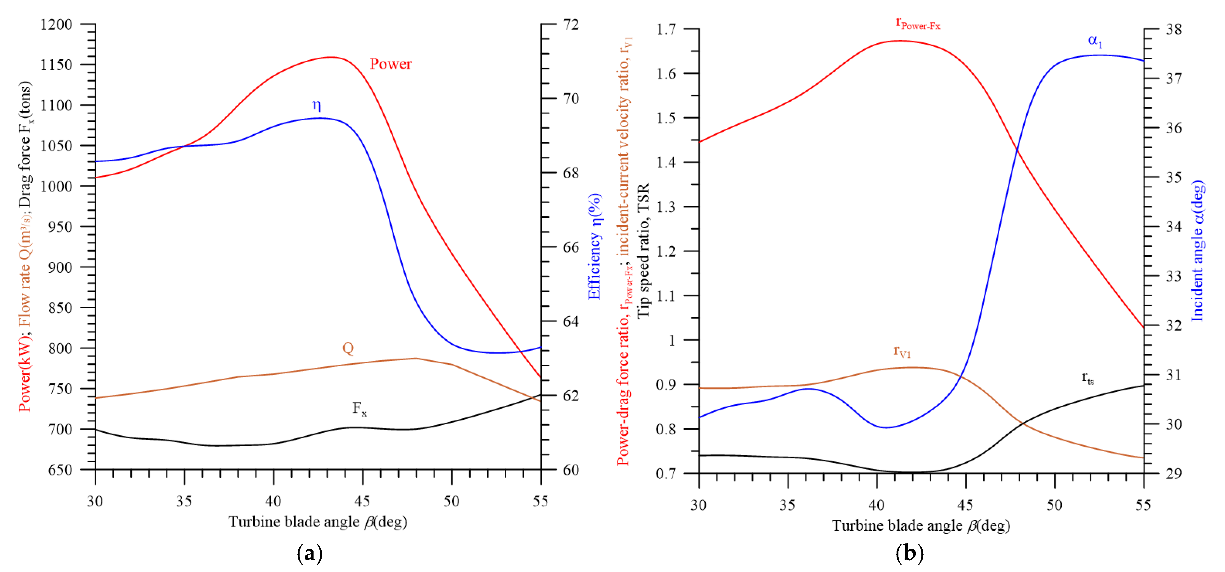
4.5. Determination of the Effect of Blade Angle on Turbine Performance Using CFD

Figure 16 demonstrates the effect of turbine blade angle β on the performance of the turbine. All parameters are the same as those in Table 1, except for those listed in

Table 4. Parameter specifications for Figure 16.

Parameter	Dimension
Channel horizontal width L1	36.69 m
Distance from turbine center to channel inlet L2	8.47 m
Distance of turbine center L4	7.875 m
Channel vertical length W0	55.63 m
Length of turbine shaft Wshaft	51.5 m
Setting angle of three blades γ1/γ2/γ3	55°/63°/50°

.

As shown in Figure 16a, if the rotor blade angle β < 48°, the flow rate Q increases with the blade angle β. If the rotor blade angle β = 48°, the flow rate is at its maximum, Q_max = 787.36 m³/s. If the rotor blade angle β > 48°, the flow rate Q decreases with the blade angle β. If the rotor blade angle β = 44°, the power is at its maximum, Power_max = 1156 kW. Meanwhile, the efficiency is highest, η_max,cfd = 69.3%. Figure 12—generated using the empirical Formulas (22) and (23)—shows that if the blade angle β = 44°, the incident angle α₁ = 30° and the efficiency is at its highest, η_opt = 71.5%, which is slightly higher than that obtained using the CFD method, η_max,cfd = 69.3%.

Figure 16b demonstrates the effect of the rotor blade angle β on the incident angle α₁, incident velocity ratio r_V1, tip speed ratio r_ts, and power–drag ratio r_power-drag. As shown in Figure 16b, if the rotor blade angle β < 37°, the incident velocity ratio r_V1 = V₁/V_cur~0.89. If 37° < β < 40°, the incident velocity ratio r_V1 increases with the blade angle β. If 40° < β < 44°, the incident velocity ratio is at its maximum, r_V1,max~0.93, the incident angle is at its minimum, α_1,min~30°, and the power–drag ratio is at its maximum, r_{power-drag,max}~1.67. If the rotor blade angle β > 44°, the incident velocity ratio r_V1 significantly decreases with the rotor blade angle β; however, this occurs in reverse for the incident angle α₁. In conclusion, the rotor blade angle β has a significant effect on the incident angle α₁, power, flow rate Q, and efficiency η.

4.6. Determining the Effects of the Setting Angles of Guide Vanes on Turbine Performance Using CFD

Figure 17 demonstrates the effects of the setting angles {γ₁, γ₂, γ₃} of three guide vanes on the performance of the turbine. The parameters of this case are the same as those listed in Table 2, except for the blade angle β = 45°. The other setting angles are ${\gamma }_2={\gamma }_1+10°$ and ${\gamma }_3={\gamma }_1-5°$. As shown in Figure 17a, if 40° < γ₁ < 78°, the power, efficiency η, and drag force F_drag increase with the vane angle γ₁; however, the reverse occurs for the flow rate Q. When the setting angle γ₁ = 78°, the power is at its maximum, power_max = 1285.4 kW and the efficiency is at its highest, η_max = 74.62%. If the setting angle γ₁ increases from 78°, the power and efficiency η will decrease. In practice, if the setting angle γ₁ is too large, the inlet flow gate will be partly covered.

As shown in Figure 17b, if 40° < γ₁ < 78°, the incident velocity ratio r_V1 and the power–drag ratio r_power-drag increase with the setting angle γ₁; however, the reverse occurs for the incident angle α₁. When the setting angle γ₁ = 78°, the incident velocity ratio is at its maximum, r_V1,max = 1.093, the power–drag ratio is at its maximum, r_{power-drag,max} = 1.764 (kW/tons), and the incident angle is at its minimum, α_1,min = 24.0°. If the setting angle γ₁ increases above 78°, the incident velocity ratio r_V1 and the power–drag ratio r_power-drag will decrease with the setting angle γ₁, but the reverse will occur for the incident angle α₁.

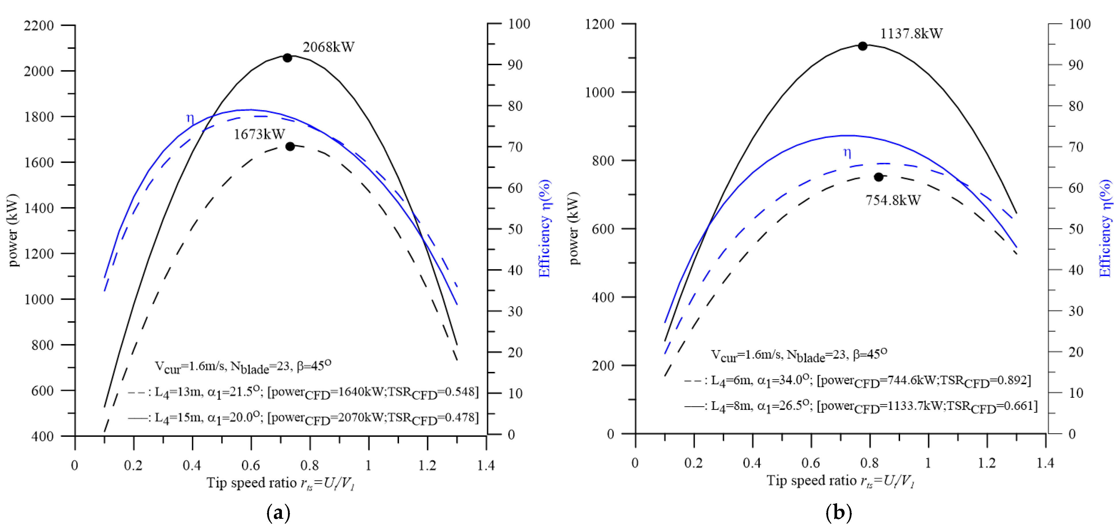
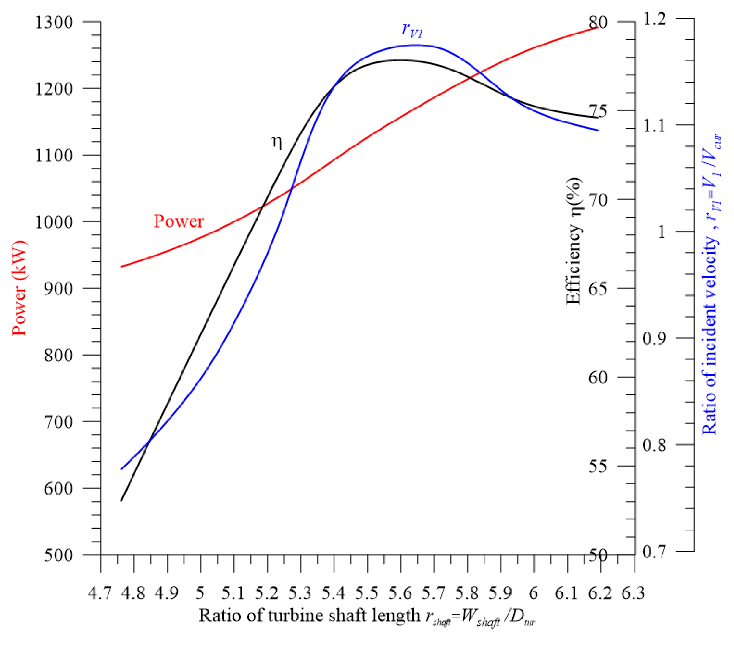
4.7. Determining the Effect of the Ratio of Turbine Shaft Length on Turbine Performance Using CFD

Figure 18 demonstrates the effect of the ratio of turbine shaft length r_shaft = W_shaft/D_tur on the performance of the turbine, where D_tur = 8.4 m. All parameters are the same as those in Table 1, except for those listed in

Table 5. Parameter specification.

Parameter	Dimension
Distance from turbine center to channel inlet L2	8.56 m
Distance from turbine center to channel outlet L3	4.66 m
Distance of two turbine centers L4	8.00
Channel vertical length W0	-
Length of turbine shaft Wshaft	-
Blade angle β	44°
Number of rotor blade Nblade	31

.

As shown in Figure 18, power increases with the ratio of turbine shaft length r_shaft. When the ratio of the turbine shaft length is increased above r_shaft = 4.762, the incident velocity ratio r_V1 also increases. If r_shaft,opt = 5.714, the incident velocity ratio is at its maximum, r_V1,max = 1.172. Meanwhile, if the ratio of turbine shaft length r_shaft is increased above 4.762, the efficiency η is also increased. If r_shaft = 5.476, the efficiency η = 77.40%. When r_shaft = 5.714, the efficiency is at its maximum, η_max = 77.54%. If r_shaft > 5.714, the efficiency η slowly decreases with the ratio of turbine shaft length. In conclusion, the optimal ratio of the turbine shaft length is approximately 5.5 < r_shaft,opt < 5.7.

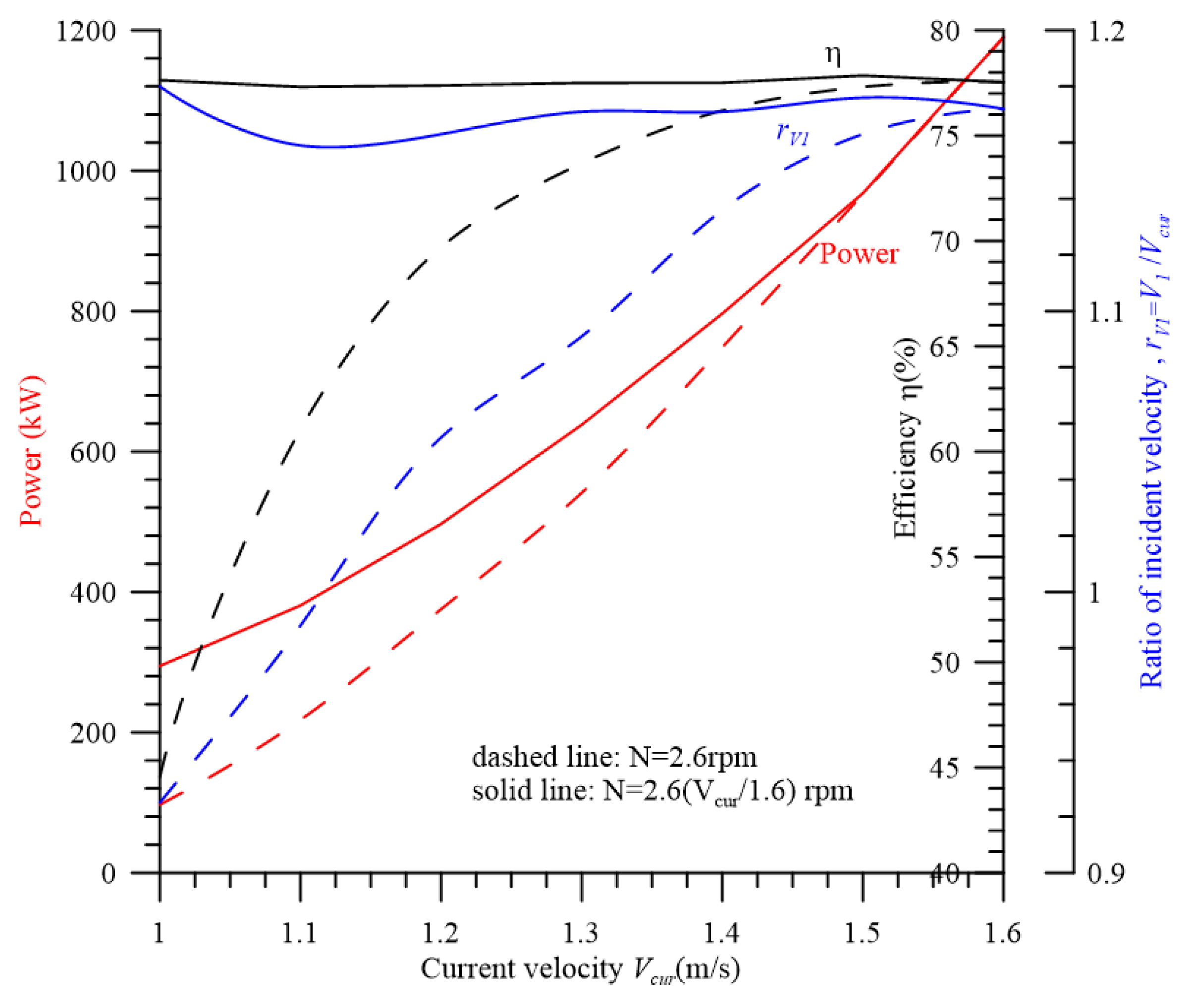
4.8. Determination of the Effect of Current Velocity on Turbine Performance Using CFD

Figure 19 demonstrates the effect of the current velocity V_cur on the performance of the turbine. All the parameters are the same as those of Figure 18, except for the current velocity V_cur and the length of the blade W_shaft = 48 m.

As shown in Figure 19, for the rotating speed N = 2.6 rpm, if the current velocity V_cur = 1.0 m/s, the power is 97.1 kW, the efficiency η = 44.54%, and the incident velocity ratio r_V1 = 0.925. The larger the current velocity V_cur is, the larger the power, incident velocity ratio r_V1, and efficiency η are. When V_cur = 1.6 m/s, the power is 1190.2 kW, the incident velocity ratio r_V1 = 1.172, and the efficiency η = 77.54%.

For the rotating speed N = 2.6 (V_cur/1.6) rpm, if the current velocity V_cur = 1.0 m/s, the power increases to 294.6 kW, the efficiency η = 77.63%, and the incident velocity ratio r_V1 = 1.180. These responses are significantly better than those obtained at a rotating speed of N = 2.6 rpm. When the rotating speed N = 2.6 (V_cur/1.6) rpm, the power, efficiency η, and incident velocity ratio r_V1 of any current velocity V_cur are increased. Moreover, whatever V_cur is, the corresponding efficiency η is about 77.5%.

5. Conclusions

A novel ocean current converter composed of two-coupled crossflow turbines is presented. The rotor, stator, and channel of the turbine are designed. The empirical formulas for calculating the power and efficiency of the converter are presented. The accuracy of these formulas is verified by comparing the theoretical results with those obtained using the CFD method. Finally, the effects of several parameters on the performance of the MW-class ocean energy converter are determined as follows:

(1)

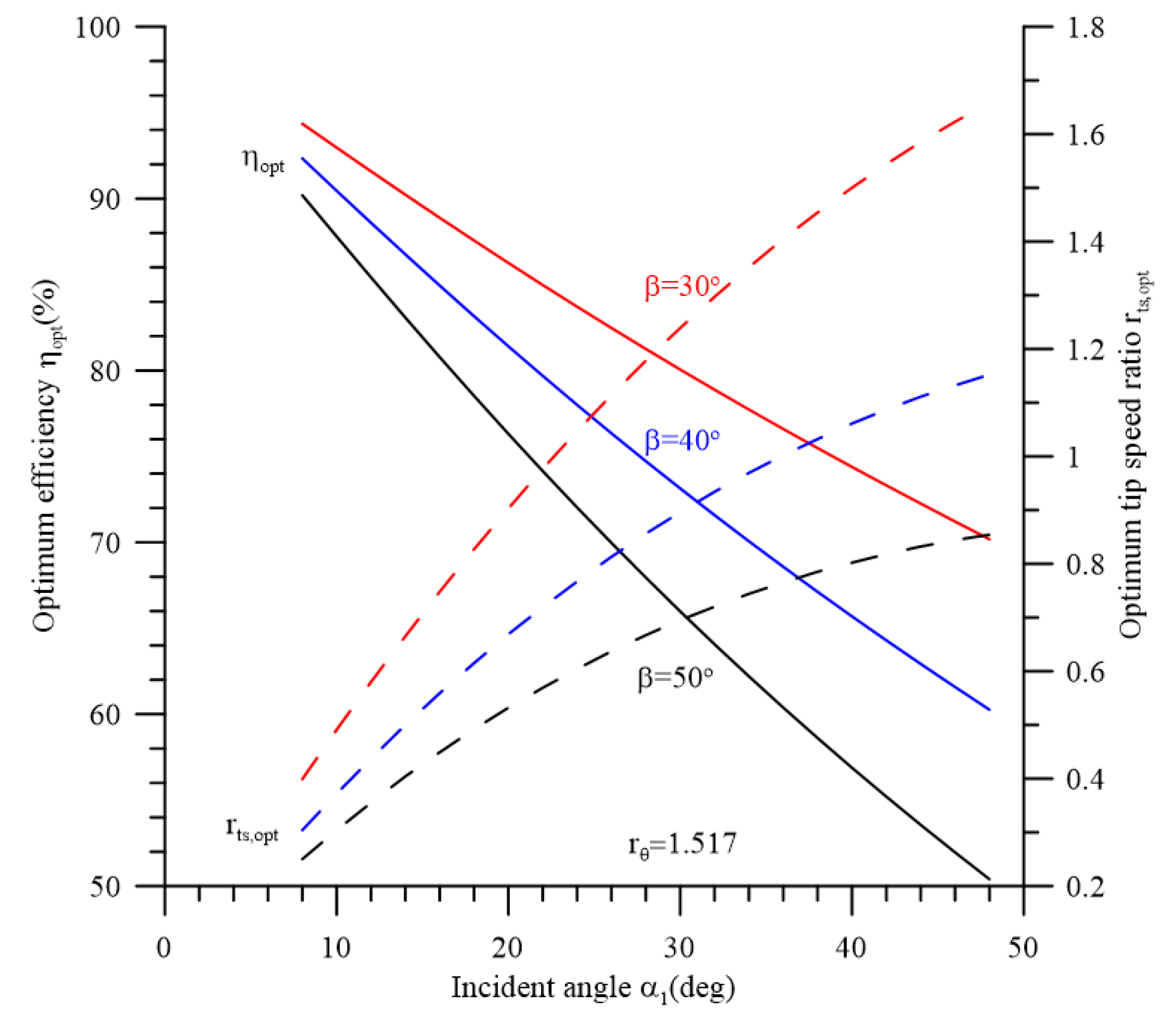
Considering the relationships of the setting angles of vanes${\gamma }_2={\gamma }_1+10°$ and ${\gamma }_3={\gamma }_1-5°$, if the setting angle γ₁ is increased, the incident angle a is decreased, and the power, efficiency η, and power–drag ratio r_power-drag are also increased. The minimum incident angle α₁ and the maximum power, efficiency η, and the power–drag ratio are obtained when γ₁ =78°. The performance of the converter decreases when the setting angle γ₁ is further increased.

(2)

If the blade angle β is increased above 30°, the flow rate Q, power, efficiency η, the power–drag ratio r_power-drag, and the incident velocity ratio r_V1 are also increased. The optimum performance is obtained when β = 44°; if the blade angle β is further increased, the performance decreases.

(3)

If the rotating speed N = 2.6 (V_cur/1.6) rpm is considered, the power, efficiency η, and incident velocity ratio r_V1 for any current velocity V_cur are significantly high. Moreover, whatever V_cur is, the corresponding efficiency η is approximately 77.5%.

(4)

The performance of each turbine with N_blade = 31 is significantly better than that with N_blade = 23.

(5)

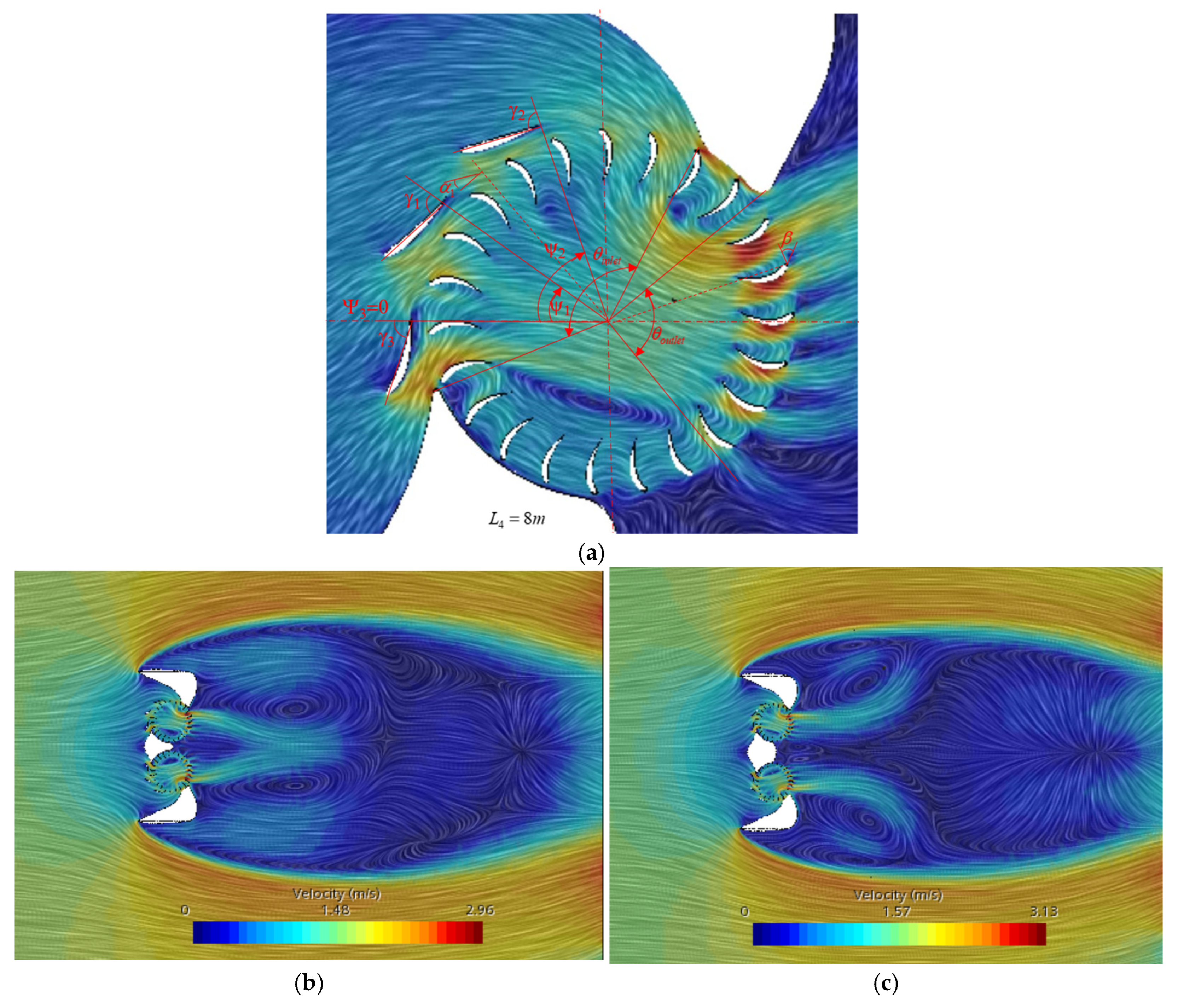
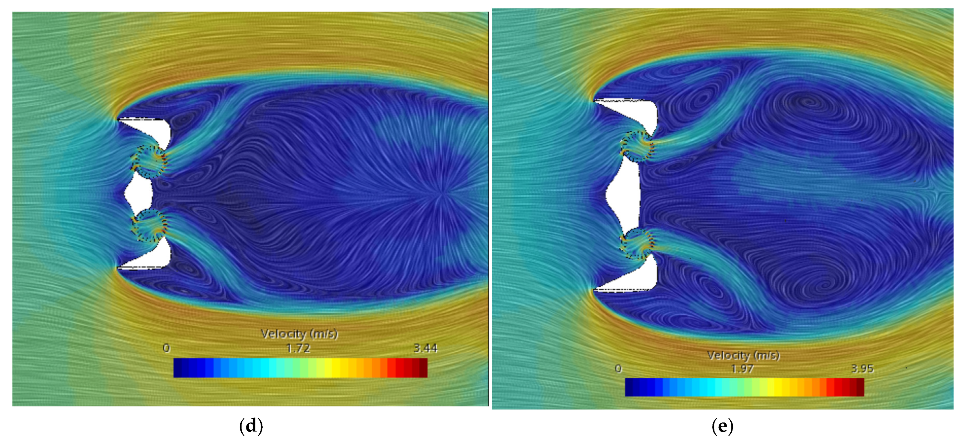
If the turbine center distance ratio r_L4 = L₄/R_o < 1.50, the efficiency η is low. Because the distance between the two turbines is too short, the outlet flows of the two turbines will interfere with each other. When r_L4 ≥ 2.50, the efficiency η is significantly high, and the two outlet flows do not interfere with each other.

(6)

The optimal ratio of the turbine shaft length is approximately 5.5 < (r_shaft = W_shaft/D_tur)_opt < 5.7.

References

1. Korte, A.; Windt, C.; Goseberg, N. Review and assessment of the German tidal energy resource. J. Ocean Eng. Mar. Energy 2024, 10, 239–261. [Google Scholar] [CrossRef]
2. Lin, S.M.; Wang, W.R.; Yuan, H. The Hydrodynamic Similarity between Different Power Levels and a Dynamic Analysis of Ocean Current Energy Converter–Platform Systems with a Novel Pulley–Traction Rope Design for Irregular Typhoon Waves and Currents. J. Mar. Sci. Eng. 2024, 12, 1670. [Google Scholar] [CrossRef]
3. Lin, S.M.; Wang, W.R.; Yuan, H. Transient translational-rotational motion of an ocean current converter mooring system with initial conditions. J. Mar. Sci. Eng. 2023, 11, 1533. [Google Scholar] [CrossRef]
4. Chen, Y.Y.; Hsu, H.C.; Bai, C.Y.; Yang, Y.; Lee, C.W.; Cheng, H.K.; Shyue, S.W.; Li, M.S. Evaluation of test platform in the open sea and mounting test of KW Kuroshio power-generating pilot facilities. In Proceedings of the 2016 Taiwan Wind Energy Conference, Keelung, Taiwan, 24–25 November 2016. [Google Scholar]
5. Zhou, Z.; Benbouzid, M.; Charpentier, J.F.; Scuiller, F.; Tang, T. Developments in large marine current turbine technologies–A review. Renew. Sustain. Energy Rev. 2017, 71, 852–858. [Google Scholar]
6. Guillou, S.S.; Eric Bibeau, E. Tidal Turbines. Energies 2023, 16, 3204. [Google Scholar] [CrossRef]
7. IHI; NEDO. The Demonstration Experiment of the IHI Ocean Current Turbine Located off the Coast of Kuchinoshima Island, Kagoshima Prefecture, Japan. 14 August 2017. Available online: https://tethys.pnnl.gov/project-sites/ihi-ocean-current-turbine (accessed on 28 August 2021).
8. Guo, J.F.; Chiu, F.C.; Tsai, J.F.; Lee, K.Y.; Li, J.H.; Hsin, C.Y. Manufacture and Sea Trial of 20 kW Floating Kuroshio Turbine; NAMR110050; Ocean Affairs Council: Kaohsiung, Taiwan, 2021. (In Chinese) [Google Scholar]
9. Zwieten, J.V.; Driscoll, F.R.; Leonessa, A.; Deane, G. Design of a prototype ocean current turbine—Part I: Mathematical modeling and dynamics simulation. Ocean Eng. 2006, 33, 1485–1521. [Google Scholar]
10. Yan, J.; Deng, X.; Korobenko, A.; Bazilevs, Y. Free-surface flow modeling and simulation of horizontal-axis tidal-stream turbines. Comput. Fluids 2017, 158, 157–166. [Google Scholar] [CrossRef]
11. Encarnacion, J.I.; Johnstone, C.; Ordonez-Sanchez, S. Design of a Horizontal Axis Tidal Turbine for Less Energetic Current Velocity Profiles. J. Mar. Sci. Eng. 2019, 7, 197. [Google Scholar] [CrossRef]
12. Kumar, M.; Nam, G.W.; Oh, S.J.; Seo, J.; Samad, A.; Hyun, S. Design Optimization of a Horizontal Axis Tidal Stream Turbine Blade Using CFD. In Proceedings of the Fifth International Symposium on Marine Propulsors SMP’17, Espoo, Finland, 12–15 June 2017. [Google Scholar]
13. Jégo, L.; Guillou, S.S. Study of a Bi-Vertical Axis Turbines Farm Using the Actuator Cylinder Method. Energies 2021, 14, 5199. [Google Scholar] [CrossRef]
14. Moreau, M.; Germain, G.; Maurice, G. Experimental performance and wake study of a ducted twin vertical axis turbine in ebb and flood tide currents at a 1/20th scale. Renew. Engergy 2023, 214, 318–333. [Google Scholar] [CrossRef]
15. Delafin, P.L.; Deniset, F.; Astolfi, J.A.; Hauville, F. Performance improvement of a Darrieus tidal turbine with active variable pitch. Energies 2021, 14, 667. [Google Scholar] [CrossRef]
16. Mockmore, C.A.; Merryfield, F. The Banki Water Turbine. In Bullettin Series, Engineering Experiment Station; Oregon State System of Higher Education, Oregon State College: Corvallis, OR, USA, 1949. [Google Scholar]
17. Sinagra, M.; Sammartanoa, V.; Aricòa, C.; Collurab, A.; Tucciarellia, T. Cross-Flow turbine design for variable operating conditions. Procedia Eng. 2014, 70, 1539–1548. [Google Scholar] [CrossRef]
18. Sinagra, M.; Sammartano, V.; Arico, C.; Collura, A. Experimental and numerical analysis of a cross-flow turbine. J. Hydraul. Eng. 2016, 142, 04015040. [Google Scholar]
19. Adanta, D.; Budiarso; Warjito; Siswantara, A.I.; Prakoso, A.P. Performance Comparison of NACA 6509 and 6712 on Pico Hydro Type Cross-Flow Turbine by Numerical Method. J. Adv. Res. Fluid Mech. Therm. Sci. 2018, 45, 116–127. [Google Scholar]
20. Sammartano, V.; Aricò, C.; Carravetta, A.; Fecarotta, O.; Tucciarelli, T. Banki-Michell Optimal Design by Computational Fluid Dynamics Testing and Hydrodynamic Analysis. Energies 2013, 6, 2362–2385. [Google Scholar] [CrossRef]
21. Woldemariam, E.T.; Lemu, H.G.; Wang, G.G. CFD-Driven Valve Shape Optimization for Performance Improvement of a Micro Cross-Flow Turbine. Energies 2018, 11, 248. [Google Scholar] [CrossRef]
22. Picone, C.; Sinagra, M.; Gurnari, L.; Tucciarelli, T.; Filianoti, P.G.F. A New Cross-Flow Type Turbine for Ultra-Low Head in Streams and Channels. Water 2023, 15, 973. [Google Scholar] [CrossRef]
23. Acharya, N.; Kim, C.G.; Thapa, B.; Lee, Y.H. Numerical analysis and performance enhancement of a cross-flow hydro turbine. Renew. Energy 2015, 80, 819–826. [Google Scholar] [CrossRef]
24. Kaya, M.; Özdemir, Y.H.; Yiğit, K.S. Investigation of a cross-flow turbine under natural conditions. Sadhana 2022, 47, 11. [Google Scholar] [CrossRef]
25. “NACA Airfoils”. nasa.gov. NASA. Available online: https://en.wikipedia.org/wiki/NACA_airfoil (accessed on 6 March 2025).
26. Lee, M.; Park, G.; Park, C.; Kim, C. Improvement of Grid Independence Test for Computational Fluid Dynamics Model of Building Based on Grid Resolution. Adv. Civ. Eng. 2020, 2020, 8827936. [Google Scholar] [CrossRef]
Figure 1. Two types of ocean current turbines (OCTs): (a) translational blade turbine (b) horizontal-axis rotational blade turbine.
Energies 18 02303 g001
Figure 2. Configuration of vertical-axis ocean current CFT converter: (a) top view; (b) side view.
Energies 18 02303 g002
Figure 3. Coordinates of the rotor blade camber.
Energies 18 02303 g003
Figure 4. Coordinates of the guide vanes.
Energies 18 02303 g004
Figure 5. Velocity triangles at the turbine inlet and outlet.
Energies 18 02303 g005
Figure 6. Procedure of CFD modeling.
Energies 18 02303 g006
Figure 7. CFD fluid regions: (a) boundary condition (b) mesh representation.
Energies 18 02303 g007
Figure 8. Effects of the total cell number Ncell on the error of numerical solution.
Energies 18 02303 g008
Figure 9. Flow fields with different turbine center distance L4: (a) local flow field with L4 = 8 m, (b) L4 = 5.0 m, (c) L4 = 6.5 m, (d) L4 = 8.0 m, and (e) L4 = 13 m.
Energies 18 02303 g009aEnergies 18 02303 g009b
Figure 10. Effect of the tip speed ratio on performance: (a) cases with L4 = 13 m, 15 m, (b) cases with L4 = 6 m, 8 m.
Energies 18 02303 g010
Figure 11. Effect of incident angle α1 on the optimum efficiency ηopt and the optimum tip speed ratio rts,opt.
Energies 18 02303 g011
Figure 12. Effect of the rotor blade angle β on the optimum efficiency ηopt and the optimum tip speed ratio rts,opt.
Energies 18 02303 g012
Figure 13. Effect of the ratio of inlet–outlet area rθ on the optimum efficiency ηopt and the optimum tip speed ratio rts,opt.
Energies 18 02303 g013
Figure 14. Effect of the ratio of turbine center distance rL4 on the performance of the converter: (a) association of rL4 = L4/Ro, power, η and Fdrag; (b) association of rL4 = L4/Ro, rts, rv1, and rpower-drag.
Energies 18 02303 g014
Figure 15. Effect of the rotating speed N on the performance of converters with different Nblade: (a) Nblade = 23, 31; association of N, power, η and Fdrag. (b) Flow field (L4 = 8 m, Nblade = 31, N = 2.6 rpm).
Energies 18 02303 g015
Figure 16. Effect of the rotor blade angle β on the performance of the turbine: (a) effect of the rotor angle β on the power, flow rate Q, and efficiency η; (b) effect of the rotor angle β on the incident angle α1, incident velocity ratio rV1, and power–drag ratio rpower-drag.
Energies 18 02303 g016
Figure 17. Effect of the setting angles {γ1, γ2, γ3} of three guide vanes on the performance of the turbine: (a) effect on the power, flow rate Q, efficiency η, and drag force Fdrag, (b) the incident angle α1, incident velocity ratio rV1, and power–drag ratio rpower-drag.
Energies 18 02303 g017
Figure 18. Effect of the ratio of the turbine shaft length rshaft on the performance of the turbine.
Energies 18 02303 g018
Figure 19. Effect of ocean current velocity on the performance of the turbine.
Energies 18 02303 g019