Detection of Cross-Line Successive Faults in Non-Effective Neutral Grounding Distribution Networks

Abstract

In a non-effectively grounded neutral point distribution network, prolonged feeder operation reduces the insulation level, thereby increasing the likelihood of single-phase grounding faults that can generate over-voltages and eventually lead to successive two-point grounding faults. Existing detection methods for single-phase grounding faults fail to identify the second grounding fault in such scenarios. This paper derives the steady-state analytical expressions for the electrical quantities during faults and examines the characteristic differences at various stages of successive grounding faults under different fault phase sequences. Based on these distinctive features, the paper proposes a detection method for successive cross-line grounding faults with varying fault phases. The effectiveness of the proposed algorithm is verified through both simulation and field data.

1. Introduction

Most medium voltage distribution networks utilize neutral point grounding via an arc suppression coil. When a single-phase grounding fault occurs, the voltage of the non-fault phase rises, which can easily lead to breakdown at weak insulation points within the non-fault phase line, potentially resulting in successive two-phase grounding faults [1,2]. If the impedance of the two-phase grounding fault circuit is low, the resulting high short-circuit current can trigger the overcurrent protection mechanism, isolating the faulted feeder. Conversely, if the impedance is high, the overcurrent protection may fail to operate. Additionally, conventional distribution networks face challenges with small-current grounding fault selection devices, including difficulties in setting the startup threshold and the inadequacy of detection methods. This often prevents the identification of a second grounding fault, hindering the rapid and accurate isolation of the faulty feeder. As a result, there may be a mistaken belief that the correctly identified first grounding fault feeder is erroneous, which can lead to unnecessary actions such as automatic line switching. This can significantly expand the impact of the fault and result in serious consequences.

Experts have conducted valuable research on the above-mentioned issue [3,4,5,6,7,8,9,10,11,12]. Starting from the fault-equivalent zero-sequence network and the compound sequence network, respectively, and by employing methods such as phasor analysis and solving differential equations, the steady-state and transient electrical quantity characteristics of successive grounding faults under different neutral grounding methods were theoretically analyzed and simulated, and the corresponding fault detection methods were proposed.

Reference [3] summarizes the key points and current status of successive fault research, including evolution mechanisms, pattern representation, scenario selection criteria, and prospects for research focus and possible breakthroughs. Reference [4] analyzed the mechanism of intermittent arc grounding transient overvoltage, which is helpful for the cause of successive faults, but did not further analyze the detection of successive faults.

References [5,6] used simulation analysis to analyze successive faults. Reference [5] simulated and analyzed the fault voltage and current characteristics of four types of successive faults—same line same phase, same line different phase, different line same phase, and different line different phase—and proposed corresponding judgment methods; Reference [6] simulated and analyzed the changes in zero sequence voltage and the current of successive faults, and selected fault lines based on the amplitude and phase of the zero sequence current characteristic frequency band. However, the above studies only provided simulation analysis, and the methods lack theoretical support, resulting in low credibility.

References [7,8,9,10] used the method of establishing an equivalent zero sequence circuit to analyze successive faults. Reference [7] calculated the transient characteristics of successive faults by constructing a zero sequence equivalent model and solving circuit differential equations, and analyzed the applicability of existing methods, but did not propose a fault detection method; Reference [8] analyzes the zero sequence equivalent network when a successive fault occurs in an ungrounded system, and obtains the variation law of the zero sequence voltage of the bus and the zero sequence current of each feeder line with the grounding resistance. Based on this, a two-stage reactive power detection method is proposed; Reference [9] proposed a two-point grounding fault protection method based on the comparison of zero sequence current amplitude and phase by analyzing the zero sequence network during successive faults in a small resistance grounding system; Reference [10] established a successive fault zero sequence equivalent model, and proposed corresponding criteria by analyzing the changes in the fault current and voltage before and after parallel resistance in the arc suppression coil. However, the method proposed in References [8,9,10] may result in missed judgments when the two grounding resistances differ significantly.

References [11,12] employed the composite sequence network method to analyze successive faults. Specifically, Reference [11] examined the characteristics of fault current and voltage changes in a neutral unground system experiencing consecutive faults of different types through a composite sequence network. It also evaluated the adaptability of existing single-phase grounding line selection methods to successive faults. However, no line selection method tailored to successive faults was proposed. In Reference [12], the composite sequence network method revealed that at least one significant difference exists—in either the magnitude or phase angle of the zero-sequence admittance—of the fault line before and after successive grounding faults occur. Based on this finding, a fault detection method was proposed. Nonetheless, this study only considered the scenarios involving B and C dependent secondary grounding, while in reality, there are cases where the phase that experiences the second grounding fault leads the phase of the first grounding fault. This method also suffers from the issue of detecting dead zones.

In summary, current research on successive faults is not comprehensive, and further investigation is urgently needed. To address this research gap, this paper refines the selection of fault scenarios. In particular, it considers a first grounding fault characterized by a relatively small transition resistance, followed by a second fault in which a high-resistance grounding fault occurs as a cross-line and different-phase successive fault. We derived analytical expressions for the fault voltage and current, and conducted a detailed analysis of the amplitude and phase changes of these parameters, especially under different fault sequences. We proposed a detection method for cross-line grounding faults in different-phase successive faults under different fault sequences, and validated the effectiveness of the algorithm through simulations and field data.

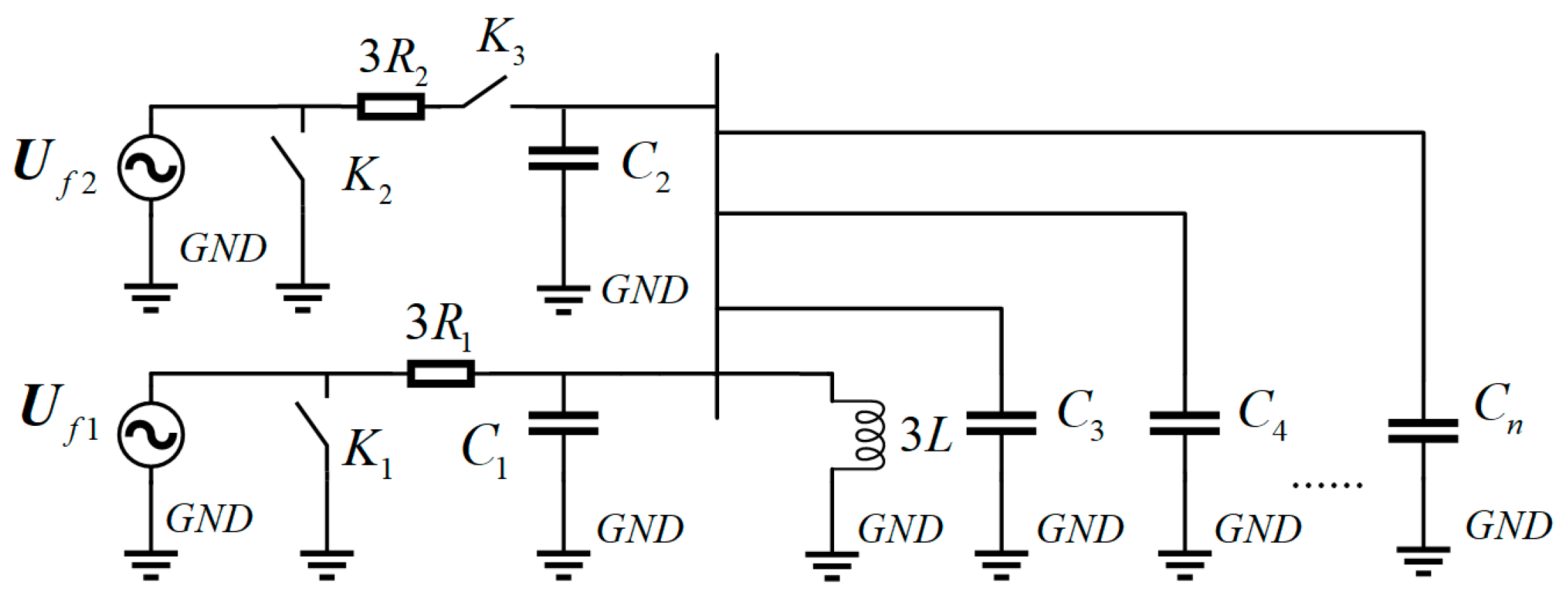
2. Modelling and Analysis of Successive Grounding Faults

Figure 1 shows the zero-sequence equivalent circuit diagram for a different-phase successive cross-line grounding fault.

Among them, U_f1 is the additional power source at fault point one, and U_f2 is the additional power source at fault point two. C_j (j = 1, 2, 3, 4, …, n) represents the zero-sequence capacitance from each feeder line to ground, and C_M denotes the total sum of these zero-sequence capacitances. L is the equivalent inductance of the arc suppression coil, while R₁ and R₂ represent the transition resistors for the two grounding faults. K₁, K₂, and K₃ are equivalent switches, and various combinations of these switches can depict the equivalent circuit for different fault scenarios.

Firstly, consider the simultaneous action of the additional power sources at the two fault points (U_f1 and U_f2), with switch K₃ closed and both K₁ and K₂ open. This configuration indicates that both points are grounded concurrently. Let U₀ represent the zero-sequence voltage, I₁₀ represent the zero-sequence current on fault line one, I₂₀ represent the zero-sequence current on fault line two, and I_j0 (j = 3, 4, …, n) represent the zero-sequence current at the outlet of an intact line. By applying the superposition theorem, the analytical expressions for the electrical quantities after the two-point grounding fault can be calculated as follows:

$$\begin{array}{l}{\mathit{U}}_0={\displaystyle \frac{{\mathit{U}}_{f1}}{3R_1+\frac{1}{j\omega C_M}//3j\omega L//3R_2}}\times {\displaystyle \frac{1}{j\omega C_M}}//3j\omega L//3R_2\\ +{\displaystyle \frac{{\mathit{U}}_{f2}}{3R_2+\frac{1}{j\omega C_M}//3j\omega L//3R_1}}\times {\displaystyle \frac{1}{j\omega C_M}}//3j\omega L//3R_1\\ ={\displaystyle \frac{j\omega L(R_2{\mathit{U}}_{f1}+R_1{\mathit{U}}_{f2})}{-3{\omega }^{2}L{C}_M{R}_1{R}_2+j\omega L(R_1+R_2)+R_1{R}_2}}\end{array}$$

(1)

$${\mathit{I}}_{j0}={\displaystyle \frac{-{\omega }^{2}L{C}_j(R_2{\mathit{U}}_{f1}+R_1{\mathit{U}}_{f2})}{-3{\omega }^{2}L{C}_M{R}_1{R}_2+j\omega L(R_1+R_2)+R_1{R}_2}}$$

(2)

$${\mathit{I}}_{10}={\displaystyle \frac{[3{\omega }^{2}L(C_M-C_1)R_2-R_2-j\omega L]{\mathit{U}}_{f1}}{-9{\omega }^{2}L{C}_M{R}_1{R}_2+3j\omega L(R_1+R_2)+3R_1{R}_2}}+{\displaystyle \frac{-3{\omega }^{2}L{C}_1{R}_1{\mathit{U}}_{f2}+j\omega L{\mathit{U}}_{f2}}{-9{\omega }^{2}L{C}_M{R}_1{R}_2+3j\omega L(R_1+R_2)+3R_1{R}_2}}$$

(3)

$${\mathit{I}}_{20}={\displaystyle \frac{[3{\omega }^{2}L(C_M-C_2)R_1-R_1-j\omega L]{\mathit{U}}_{f2}}{-9{\omega }^{2}L{C}_M{R}_1{R}_2+3j\omega L(R_1+R_2)+3R_1{R}_2}}+{\displaystyle \frac{-3{\omega }^{2}L{C}_2{R}_2{\mathit{U}}_{f1}+j\omega L{\mathit{U}}_{f1}}{-9{\omega }^{2}L{C}_M{R}_1{R}_2+3j\omega L(R_1+R_2)+3R_1{R}_2}}$$

(4)

The detailed derivation of Equations (1)–(4) is shown in Appendix A.

Next, consider the case where the switches K₁ and K₃ are disconnected to analyze the characteristics of a single-point, single-phase grounding fault. In this scenario, let U_0s denote the zero-sequence voltage, I_10s the zero-sequence current on fault line one, and I_20s the zero-sequence current on fault line two (which acts as a healthy line during the single-point, single-phase grounding fault). Thus, we have:

$${\mathit{U}}_{0s}={\displaystyle \frac{j\omega L{\mathit{U}}_{f1}}{j\omega L+R_1-3{\omega }^{2}L{C}_M{R}_1}}$$

(5)

$${\mathit{I}}_{10s}={\displaystyle \frac{[3{\omega }^2(C_M-C_1)L-1]{\mathit{U}}_{f1}}{3j\omega L+3R_1-9{\omega }^{2}L{C}_M{R}_1}}$$

(6)

$${\mathit{I}}_{20s}={\displaystyle \frac{-{\omega }^2{C}_{2}L{\mathit{U}}_{f1}}{j\omega L+R_1-3{\omega }^{2}L{C}_M{R}_1}}$$

(7)

3. Changes in Electrical Quantity Characteristics of Successive Grounding Faults

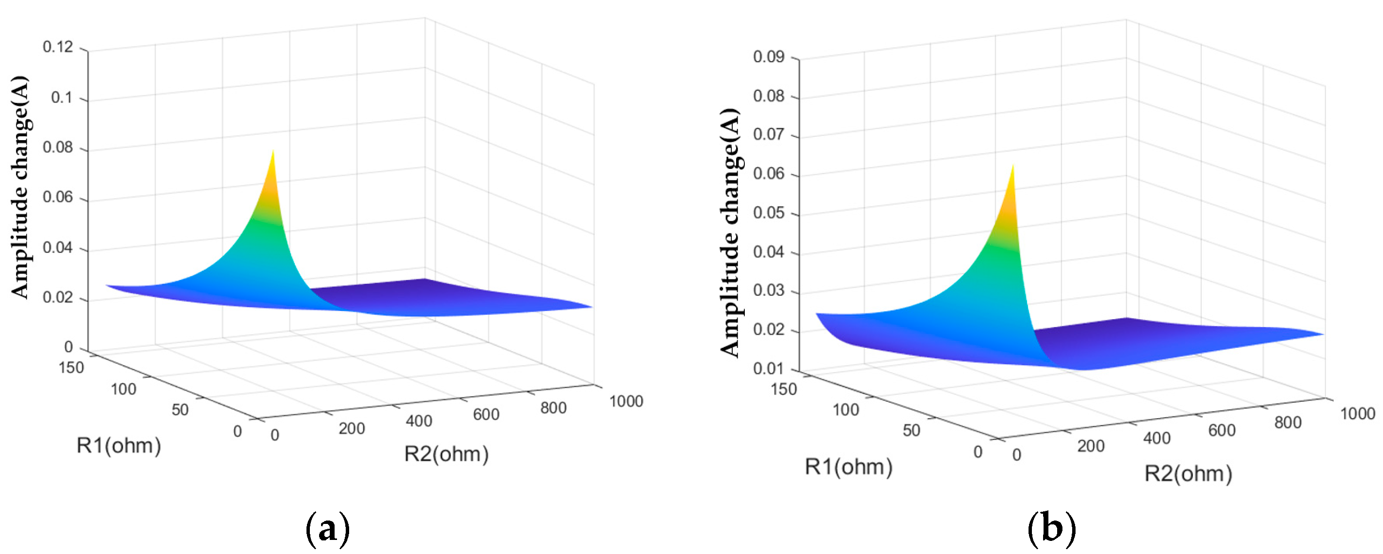
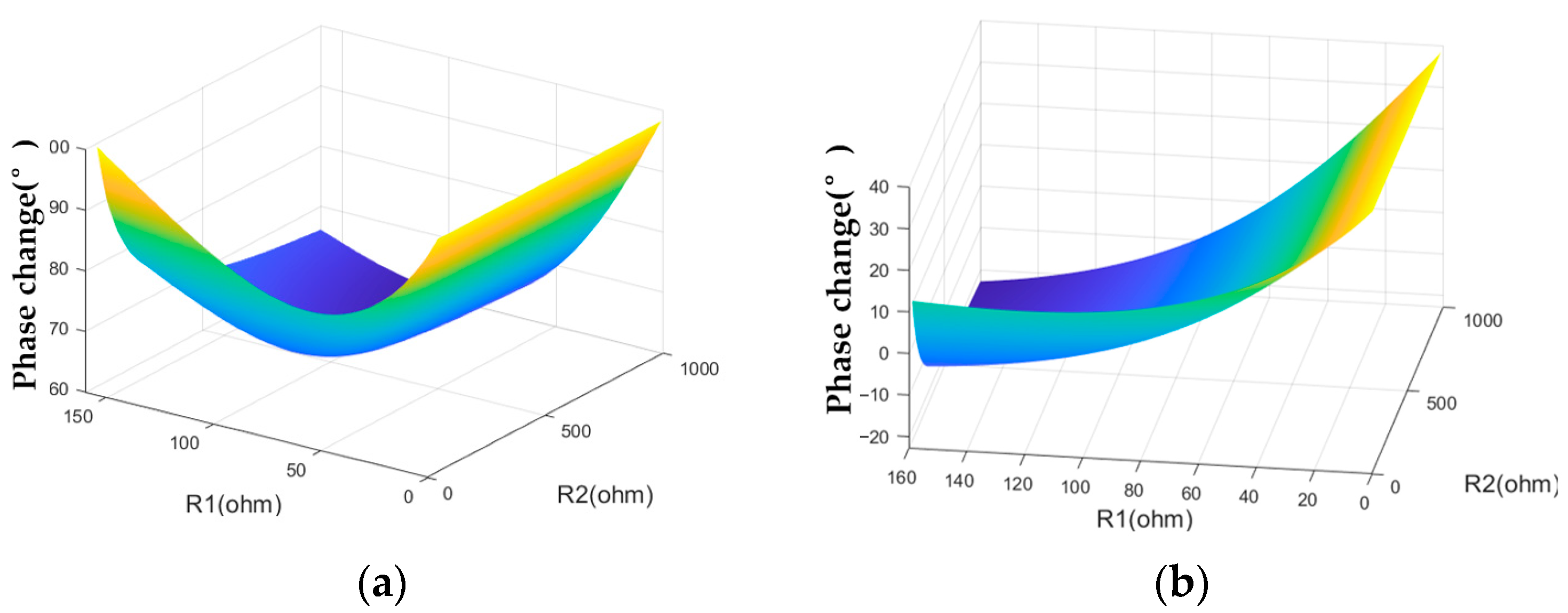
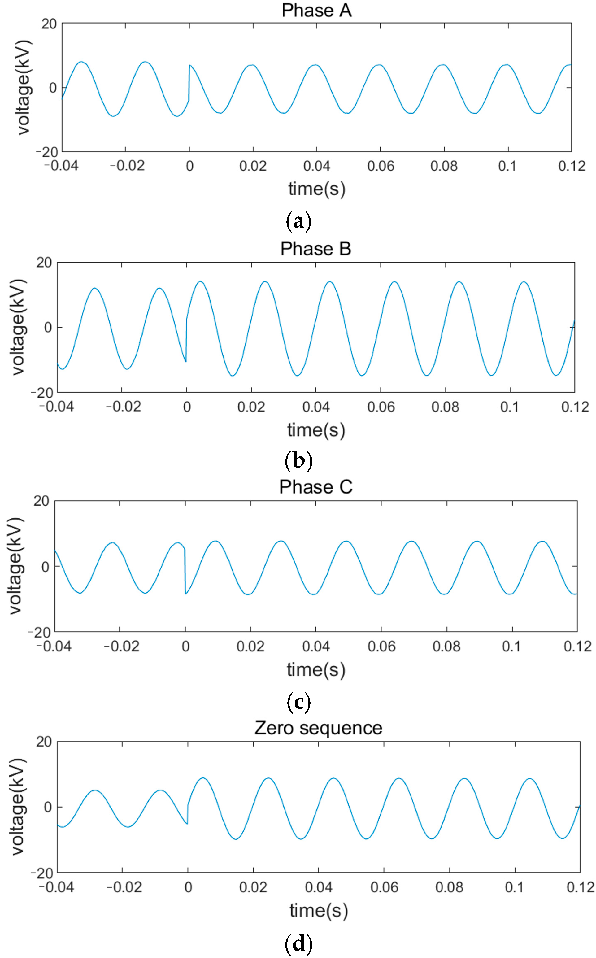
3.1. Fault Characteristic Analysis

In order to quantify the characteristic changes, analyze the difference in electrical quantities as a single-point, single-phase grounding fault evolves into a successive grounding fault. Specifically, define the electrical changes ΔU₀, ΔI₁₀, and ΔI₂₀ as the differences in voltage and current phasors between the single-point, single-phase grounding fault and the two-point, single-phase grounding fault, respectively.

$$\begin{array}{l}\mathrm{\Delta }{\mathit{U}}_0={\mathit{U}}_{0s}-{\mathit{U}}_0\\ ={\displaystyle \frac{j\omega L{\mathit{U}}_{f1}}{j\omega L+R_1-3{\omega }^{2}L{C}_M{R}_1}}-{\displaystyle \frac{j\omega L(R_2{\mathit{U}}_{f1}+R_1{\mathit{U}}_{f2})}{-3{\omega }^{2}L{C}_M{R}_1{R}_2+j\omega L(R_1+R_2)+R_1{R}_2}}\end{array}$$

(8)

$$\begin{array}{l}\mathrm{\Delta }{\mathit{I}}_{10}={\mathit{I}}_{10s}-{\mathit{I}}_{10}\\ ={\displaystyle \frac{[3{\omega }^2(C_M-C_1)L-1]{\mathit{U}}_{f1}}{3j\omega L+3R_1-9{\omega }^{2}L{C}_M{R}_1}}-{\displaystyle \frac{[3{\omega }^{2}L(C_M-C_1)R_2-R_2-j\omega L]{\mathit{U}}_{f1}}{-9{\omega }^{2}L{C}_M{R}_1{R}_2+3j\omega L(R_1+R_2)+3R_1{R}_2}}\\ -{\displaystyle \frac{-3{\omega }^{2}L{C}_1{R}_1{\mathit{U}}_{f2}+j\omega L{\mathit{U}}_{f2}}{-9{\omega }^{2}L{C}_M{R}_1{R}_2+3j\omega L(R_1+R_2)+3R_1{R}_2}}\end{array}$$

(9)

$$\begin{array}{l}\mathrm{\Delta }{\mathit{I}}_{20}={\mathit{I}}_{20s}-{\mathit{I}}_{20}\\ ={\displaystyle \frac{-{\omega }^2{C}_{2}L{\mathit{U}}_{f1}}{j\omega L+R_1-3{\omega }^{2}L{C}_M{R}_1}}-{\displaystyle \frac{[3{\omega }^{2}L(C_M-C_2)R_1-R_1-j\omega L]{\mathit{U}}_{f2}}{-9{\omega }^{2}L{C}_M{R}_1{R}_2+3j\omega L(R_1+R_2)+3R_1{R}_2}}\\ -{\displaystyle \frac{-3{\omega }^{2}L{C}_2{R}_2{\mathit{U}}_{f1}+j\omega L{\mathit{U}}_{f1}}{-9{\omega }^{2}L{C}_M{R}_1{R}_2+3j\omega L(R_1+R_2)+3R_1{R}_2}}\end{array}$$

(10)

Based on the research scenario in this article, if we assume that the second grounding fault employs high impedance grounding (i.e., R₂ >> R₁), and noting that jωLR₂ ≈ jωL (R₁ + R₂), then Equations (8) through (10) can be further simplified as:

$$\mathrm{\Delta }{\mathit{U}}_0\approx {\displaystyle \frac{-j\omega L{R}_1{\mathit{U}}_{f2}}{(1-3{\omega }^{2}L{C}_M)R_1{R}_2+j\omega L(R_1+R_2)}}$$

(11)

$$\mathrm{\Delta }{\mathit{I}}_{10}\approx {\displaystyle \frac{3{\omega }^{2}L{C}_1{R}_1{\mathit{U}}_{f2}+j\omega L({\mathit{U}}_{f1}-{\mathit{U}}_{f2})}{(3-9{\omega }^{2}L{C}_M)R_1{R}_2+3j\omega L(R_1+R_2)}}$$

(12)

$$\mathrm{\Delta }{\mathit{I}}_{20}\approx {\displaystyle \frac{[1-3{\omega }^{2}L(C_M-C_2)]R_1{\mathit{U}}_{f2}+j\omega L({\mathit{U}}_{f2}-{\mathit{U}}_{f1})}{(3-9{\omega }^{2}L{C}_M)R_1{R}_2+3j\omega L(R_1+R_2)}}$$

(13)

The amplitude of ΔU₀ in Equation (11) is:

$$|\mathrm{\Delta }{\mathit{U}}_0|\approx \sqrt{{\displaystyle \frac{{(\omega L)}^2}{{[(1-3{\omega }^{2}L{C}_M)R_2]}^2+{[\omega L(1+R_2/R_1)]}^2}}}|{\mathit{U}}_{f2}|$$

(14)

It can be seen that with the determination of distribution line parameters, the amplitude of ΔU₀ increases with the increase in R₁ and decreases with the increase in R₂.

Further calculate the phase of Equation (11) ΔU₀:

$$\phi (\mathrm{\Delta }{\mathit{U}}_0)\approx -{90}^{\circ }-\arctan ({\displaystyle \frac{\omega L(R_1+R_2)}{(1-3{\omega }^{2}L{C}_M)R_1{R}_2}})+\phi ({\mathit{U}}_{f2})$$

(15)

By substituting the typical distribution line parameter values [13] (see Section 3.2 for specific parameters), it can be seen that the expression (1 − 3ω²LC_M) is numerically negative. Therefore, let:

$$\left\{\begin{array}{l}f(R_1,R_2)={\displaystyle \frac{\omega L(R_1+R_2)}{k{R}_1{R}_2}}\\ k=(1-3{\omega }^{2}L{C}_M)<0\end{array}\right.$$

(16)

The functions f(R₁, R₂) take the derivatives of R₁ and R₂, respectively, and obtain:

$$\left\{\begin{array}{l}{\displaystyle \frac{\partial f(R_1,R_2)}{\partial R_1}}=-{\displaystyle \frac{\omega L}{k{R_1}^2}}>0\\ {\displaystyle \frac{\partial f(R_1,R_2)}{\partial R_2}}=-{\displaystyle \frac{\omega L}{k{R_2}^2}}>0\end{array}\right.$$

(17)

f(R₁, R₂) increases as R₁ and R₂ increase, and according to Equation (15), the ΔU₀ phase decreases with the increases in R₁ and R₂.

By substituting typical distribution line parameter values, the values of expressions 3ω²LC₁R₁U_f2 and [1 − 3ω²L(C_M − C₂)]R₁U_f2 in Equations (12) and (13) are significantly smaller than the imaginary part of the molecule, so they can be discarded. Similarly, it can be seen that the amplitude and phase of ΔI₁₀ and ΔI₂₀ decrease monotonically with the increases in R₁ and R₂. Therefore, the amplitude or phase change of zero sequence voltage or the detected fault line zero sequence current can be used as the starting criterion for successive grounding fault detection.

The above description illustrates that the electrical quantities on a faulty line vary as a function of the transition resistance. However, an effective method for distinguishing between faulty and healthy lines still needs to be developed. According to Equations (1), (4), (5) and (7), the amplitude variations of the zero-sequence current and zero-sequence voltage on a healthy line are essentially identical, with the zero-sequence current’s phase consistently leading that of the zero-sequence voltage by 90°. Therefore, the more readily accessible zero-sequence voltage is adopted as a substitute for the zero-sequence current on the healthy line as a reference. Subsequently, by analyzing the difference in either the amplitude or phase changes between the zero-sequence current and zero-sequence voltage on the second faulty line, the faulty line can be effectively identified.

It is observed that Equations (12) and (13) contain the term (U_f1 − U_f2), which indicates that the fault phase sequence affects the phase and amplitude variations of the zero-sequence current in the faulted line. Therefore, it is necessary to analyze different fault phase sequences separately. Specifically, when the second grounding fault lags 120° behind the first grounding fault, it is defined as a sequential grounding fault; conversely, if the second grounding fault leads the first grounding fault by 120°, it is termed a reverse sequence grounding fault.

According to Equations (5), (7), (11) and (13), the difference in the amplitude changes of electrical quantities can be calculated, denoted as ΔB, as shown in Equation (18).

$$\mathrm{\Delta }\mathit{B}={\displaystyle \frac{j}{\omega C_x}}\mathrm{\Delta }{\mathit{I}}_{x0}-\mathrm{\Delta }{\mathit{U}}_0$$

(18)

Among them, the subscript x represents the line number.

ΔB represents the conversion of the zero-sequence current change into the same unit as the zero-sequence voltage change, followed by the calculation of the difference between the two. For a healthy power line, since the zero-sequence current and zero-sequence voltage are proportional, the value of |ΔB| is zero. Considering practical measurement errors, its value should be close to zero. Thus, this characteristic can be effectively used to distinguish between faulty and healthy lines.

By substituting Equations (11) and (13), calculate the difference between the zero-sequence current change and zero sequence voltage change of fault line 2, and obtain Equation (19):

$$\mathrm{\Delta }\mathit{B}={\displaystyle \frac{-\omega L({\mathit{U}}_{f2}-{\mathit{U}}_{f1})+j[1-3{\omega }^{2}L(C_M-2C_2)]R_1{\mathit{U}}_{f2}}{(3-9{\omega }^{2}L{C}_M)\omega C_2{R}_1{R}_2+3j{\omega }^{2}L{C}_2(R_1+R_2)}}$$

(19)

Equation (19) takes the parameter values and takes the derivatives of R₁ and R₂, respectively. It is found that the value of |ΔB| decreases with the increase in R₁ and R₂. At the same time, it can be found that there is a term (U_f2 − U_f1) in Equation (19), indicating that the fault phase sequence will affect the value of |ΔB|.

Furthermore, according to Equations (11) and (13), analyze the difference in phase variation between the zero-sequence current and zero sequence voltage of the fault line 2, denoted as Δφ, as shown in Equation (20):

$$\mathrm{\Delta }\phi =\phi (\mathrm{\Delta }{\mathit{I}}_{20})-\phi (\mathrm{\Delta }{\mathit{U}}_0)\approx \left\{\begin{array}{l}\arctan ({\displaystyle \frac{\sqrt{3}\omega L+2m{R}_1}{3\omega L}}), \mathrm{Sequential}\\ \arctan ({\displaystyle \frac{-\sqrt{3}\omega L+2m{R}_1}{3\omega L}}), \mathrm{Reverse} \mathrm{Sequential}\end{array}\right.$$

(20)

Among them

$$m=1-3{\omega }^{2}L(C_M-C_2)<0$$

(21)

Analysis shows that Δφ depends only on R₁ and is independent of R₂, and the fault phase sequence will have a significant impact on Δφ.

When addressing the fixed-value setting issue, the first step is to determine the variation range of the grounding resistors R₁ and R₂ based on the on-site conditions. According to the fault scenario discussed in this paper, it is recommended to treat the first fault as a low-resistance grounding fault and the second fault as a high-resistance grounding fault. For different fault phase sequences, sequential grounding faults and reverse grounding faults occur in phases B and C, and phases B and A, respectively. The next step is to substitute the parameters into Equations (12), (19) and (20) to calculate the minimum amplitude of ΔI₁₀, the corresponding phase change interval, the minimum value of |ΔB|, and the variation range of Δφ These calculated values are then used to determine the fixed-setting value, with the specific setting method detailed in Section 4.1.

3.2. Simulation Analysis of Fault Characteristics

As shown in Figure 2, a fault simulation model of a 10 kV medium voltage distribution network with a neutral point grounded through an arc suppression coil was built using the PSCAD 4.6.2 simulation software, and the compensation degree of the arc suppression coil was 8%. It includes four feeders, with Line 1 consisting of 3 km cables and 1 km overhead lines, Line 2 consisting of 6 km cables, Line 3 consisting of 2 km cables and 2.5 km overhead lines, and Line 4 consisting of 10 km overhead lines. The parameters of cables and overhead lines are shown in

Table 1. Model line parameters.

Line Type	R1 (Ω/km)	C1 (μF/km)	L1 (mH/km)	R0 (Ω/km)	C0 (μF/km)	L0 (mH/km)
Overhead line	0.1700	0.0097	1.2096	0.23	0.006	5.4749
Cable	0.2700	0.3390	0.2550	0.27	0.280	1.0190

. Fault F1 occurs at a distance of 2 km from the busbar on Line 3, and fault F2 occurs at a distance of 3 km from the busbar on Line 1.

Based on the topology in Figure 2, a simulation analysis was performed on the changes in electrical quantities when a single-point single-phase grounding fault develops into a successive grounding fault. Using the simulation model parameters, the following values were obtained: L = 0.844H, C₁ = 2.86 × 10⁻⁶F, C₂ = 2.818 × 10⁻⁶F, C_M = 1.1118 × 10⁻⁵F. In the subsequent analysis, R₁ is varied from 1 to 150 Ω and R₂ from 50 to 1000 Ω. (Note that the variation in resistance values does not affect the fault detection principle; it only influences the setting of the constant value, which can be chosen based on actual field conditions.) The amplitude and phase variations of ΔI₁₀ (i.e., the zero-sequence voltage variation on the faulted line) for sequential and reverse grounding faults are illustrated in Figure 3 and Figure 4, respectively.

By analyzing Figure 3 and Figure 4, the characteristics of the zero-sequence current variation on the faulted line, as shown in

Table 2. Comparison of changes in ΔI₁₀ under different fault phase sequences.

ΔI10	Characteristic	Sequential Grounding	Reverse Sequential Grounding
Amplitude variation	As R1 increases	Reduce	Reduce
	As R2 increases	Reduce	Reduce
	Maximum value	86.6 A	90.4 A
	Minimum value	1.0 A	2.2 A
Phase change	As R1 increases	Reduce first and then increase	Reduce
	As R2 increases	Reduce	Reduce
	Maximum value	98.9°	38.3°
	Minimum value	61.2°	−22.8°

, can be derived. A comparison between sequential grounding and reverse grounding reveals that the overall phase change of ΔI₁₀ is higher in sequential grounding than in reverse grounding, while the amplitude of ΔI₁₀ remains consistently above zero. This confirms that the fault phase sequence indeed affects the fault characteristics.

According to Table 2, the minimum value of ΔI₁₀ amplitude change of 1.0 A under two fault phase sequences can be taken as the starting criterion for successive grounding fault detection, and the point value of 50° in the ΔI₁₀ phase change interval under two fault phase sequences can be taken as the fault phase sequence detection criterion.

Furthermore, plot the variation of |ΔB| under different fault phase sequences as shown in Figure 5. It can be seen that the minimum value of |ΔB| is 1.7 kV under sequential grounding and 3.0 kV under reverse grounding.

Draw the variation of Δφ, as shown in Figure 6 for different fault phase sequences. The results indicate that the phase variation range is [−184.5°, −124.0°] for sequential grounding, and [185.5°, 236.4°] for reverse grounding.

Therefore, detection criteria can be established based on the fault phase sequence. In the case of sequential grounding, inspect the line, and if it meets the conditions that the change in |ΔB| exceeds 1.7 kV and Δφ falls within the range [−184.5°, −124.0°], then it is identified as the second grounding line. Conversely, in the case of reverse grounding, if a line exhibits a |ΔB| change greater than 3.0 kV with Δφ within the range [185.5°, 236.4°], it is similarly judged to be the second grounding line.

4. Detection Method for Cross Line Successive Grounding Faults

4.1. Detection Method

Based on the above criteria for detecting the characteristics of successive cross line faults with different names, the following fault detection methods are proposed:

(1)

Firstly, select the first single-phase grounded fault line and fault phase using traveling wave method or transient method [1,14].

(2)

Real-time monitoring of zero sequence current and zero sequence voltage of each line, denoted as I_0j(t) and U₀(t), with the single-phase grounding time denoted as t₀. If at a certain time t1, the zero sequence current of the first faulty line satisfies |I_0f(t₀) − I_0f(t₁)| > k, then proceed to step (3), otherwise return to step (1).

(3)

Determine whether it satisfies the condition of φ(I_0f(t₀)) φ(I_0f(t₁)) > g. If so, proceed to step (4), otherwise, proceed to step (5).

(4)

Continue to inspect the remaining lines. If a certain line satisfies |ΔB_x| > b₁ and p₁ < Δφ_x < q₁, it is considered as fault line two, and its fault phase is the phase that lags 120° behind the first fault phase. Then, proceed to step (6).

(5)

Continue to inspect the remaining lines. If a certain line satisfies |ΔB_x| > b₂ and p₂ < Δφ_x < q₂, then the line is fault line two, and its fault phase is the phase that leads the first fault phase by 120°. Enter step (6).

(6)

Exit trip or alarm, end.

The algorithm flowchart is shown in Figure 7.

The fixed values k, g, b₁, p₁, q₁, b₂, p₂, q₂ in the detection method can be calculated as follows.

Using the amplitude change of ΔI₁₀ as the fault initiation criterion, the fixed value k is calculated according to Equation (22), representing the smaller of the minimum amplitude change of ΔI₁₀ for sequential grounding and the minimum amplitude change of ΔI₁₀ for reverse grounding.

$$k=a_1\times \min \{\min |\mathrm{\Delta }{\mathit{I}}_{10}{|}_{\mathrm{seq}}, \min |\mathrm{\Delta }{\mathit{I}}_{10}{|}_{\mathrm{r}-\mathrm{seq}}\}$$

(22)

Among them, seq represents the sequential grounding situation and r-seq represents the reverse grounding situation.

Using the phase change of ΔI₁₀ as the fault initiation criterion, since the overall phase change of ΔI₁₀ during sequential grounding is higher than that during reverse grounding, the average of the maximum and minimum phase changes during reverse grounding is taken as the phase sequence criterion. Criterion g can be calculated according to Equation (23).

$$g={\displaystyle \frac{1}{2}}(\max \phi {(\mathrm{\Delta }{\mathit{I}}_{10})}_{\mathrm{r}-\mathrm{seq}}+\min \phi {(\mathrm{\Delta }{\mathit{I}}_{10})}_{\mathrm{seq}})$$

(23)

As shown in Figure 4, |ΔB| is always greater than zero, so b₁ and b₂ take the minimum values of |ΔB| for sequential grounding and reverse grounding, respectively, as shown in Equation (24).

$$\left\{\begin{array}{l}{b}_1=a_2\times \min {(|\mathrm{\Delta }\mathit{B}|)}_{\mathrm{seq}}\\ b_2=a_3\times \min {(|\mathrm{\Delta }\mathit{B}|)}_{\mathrm{r}-\mathrm{seq}}\end{array}\right.$$

(24)

p₁, q₁, p₂, and q₂ are, respectively, adjusted according to the variation interval of Δφ, as shown in Equation (25):

$$\left\{\begin{array}{l}{p}_1=a_4\times \min {(\mathrm{\Delta }\phi )}_{\mathrm{seq}},q_1=a_5\times \max {(\mathrm{\Delta }\phi )}_{\mathrm{seq}}\\ p_2=a_6\times \min {(\mathrm{\Delta }\phi )}_{\mathrm{r}-\mathrm{seq}},q_2=a_7\times \max {(\mathrm{\Delta }\phi )}_{\mathrm{r}-\mathrm{seq}}\end{array}\right.$$

(25)

In Equations (22)–(25), a₁~a₇ are setting coefficients, which can be adjusted according to the actual situation on site. It is recommended to take a₁ = 0.9, a₂ = 0.9, a₃ = 0.9, a₄ = 1.1, a₅ = 0.9, a₆ = 0.9, a₇ = 1.1.

4.2. Interference Analysis

The previous analysis indicated that the first grounding fault is stable; however, if the initial fault becomes unstable, both the zero-sequence current and voltage will change. The following analysis will evaluate the anti-interference capability of the proposed method. The core idea of the method is to ensure that the variation in zero-sequence current is consistent with that of the zero-sequence voltage in a sound line, using fixed thresholds to identify faulted lines. Therefore, it is crucial to analyze whether changes in fault conditions could affect this conclusion.

The first aspect distinguishes between unstable single-phase grounding faults and successive faults: When an unstable single-phase grounding fault occurs, the current amplitude and phase of the faulty line will change. However, for all other (sound) lines, the trend in the variation of the zero-sequence current remains consistent with that of the zero-sequence voltage. As a result, there is no risk of mistakenly identifying a sound line as exhibiting a secondary grounding fault.

It is worth noting that the single-phase grounding transition resistance is R₁ before the change and R_1n after the change. Calculate the changes in various electrical quantities as follows:

$$\mathrm{\Delta }{\mathit{U}}_0={\mathit{U}}_{0s}(R_1)-{\mathit{U}}_{0s}(R_{1n})={\displaystyle \frac{j\omega L{\mathit{U}}_{f1}}{j\omega L+R_1-3{\omega }^{2}L{C}_M{R}_1}}-{\displaystyle \frac{j\omega L{\mathit{U}}_{f1}}{j\omega L+R_{1n}-3{\omega }^{2}L{C}_M{R}_{1n}}}$$

(26)

$$\mathrm{\Delta }{\mathit{I}}_{10}={\mathit{I}}_{10s}(R_1)-{\mathit{I}}_{10s}(R_{1n})={\displaystyle \frac{[3{\omega }^2(C_M-C_1)L-1]{\mathit{U}}_{f1}}{3j\omega L+3R_1-9{\omega }^{2}L{C}_M{R}_1}}-{\displaystyle \frac{[3{\omega }^2(C_M-C_1)L-1]{\mathit{U}}_{f1}}{3j\omega L+3R_{1n}-9{\omega }^{2}L{C}_M{R}_{1n}}}$$

(27)

$$\mathrm{\Delta }{\mathit{I}}_{j0}={\mathit{I}}_{j0s}(R_1)-{\mathit{I}}_{j0s}(R_{1n})=j\omega C_j\mathrm{\Delta }{\mathit{U}}_0$$

(28)

From Equation (30), it can be inferred that:

$$\mathrm{\Delta }{B}_j={\displaystyle \frac{j}{\omega C_j}}\mathrm{\Delta }{\mathit{I}}_{j0}-\mathrm{\Delta }{\mathit{U}}_0=0$$

(29)

$$\mathrm{\Delta }{\phi }_j=\phi (\mathrm{\Delta }{\mathit{I}}_{j0})-\phi (\mathrm{\Delta }{\mathit{U}}_0)=90°$$

(30)

Based on the above analysis, unstable single-phase grounding faults can lead to fluctuations in the zero-sequence current on the faulty grounding line, potentially triggering a determination of a successive fault. However, as demonstrated by Equations (29) and (30), the amplitude and phase variation trends of the zero-sequence current in the intact line remain consistent with those of the zero-sequence voltage. Consequently, this consistency prevents the misidentification of a second faulted grounding line.

The second aspect is that for successive faults, if the transition resistance of the first grounding fault changes, analyze whether this situation will affect the judgment of the second faulty line.

Calculate the changes in various electrical quantities as follows:

$$\begin{array}{l}\mathrm{\Delta }{\mathit{U}}_0={\mathit{U}}_{0s}(R_1)-{\mathit{U}}_0(R_{1n},R_2)\\ ={\displaystyle \frac{j\omega L{\mathit{U}}_{f1}}{j\omega L+R_1-3{\omega }^{2}L{C}_M{R}_1}}-\\ {\displaystyle \frac{j\omega L(R_2{\mathit{U}}_{f1}+R_{1n}{\mathit{U}}_{f2})}{-3{\omega }^{2}L{C}_M{R}_{1n}{R}_2+j\omega L(R_{1n}+R_2)+R_{1n}{R}_2}}\end{array}$$

(31)

$$\begin{array}{l}\mathrm{\Delta }{\mathit{I}}_{10}={\mathit{I}}_{10s}(R_1)-{\mathit{I}}_{10}(R_{1n},R_2)\\ ={\displaystyle \frac{[3{\omega }^2(C_M-C_1)L-1]{\mathit{U}}_{f1}}{3j\omega L+3R_1-9{\omega }^{2}L{C}_M{R}_1}}-\\ {\displaystyle \frac{[3{\omega }^{2}L(C_M-C_1)R_2-R_2-j\omega L]{\mathit{U}}_{f1}}{-9{\omega }^{2}L{C}_M{R}_{1n}{R}_2+3j\omega L(R_{1n}+R_2)+3R_{1n}{R}_2}}\\ -{\displaystyle \frac{-3{\omega }^{2}L{C}_1{R}_{1n}{\mathit{U}}_{f2}+j\omega L{\mathit{U}}_{f2}}{-9{\omega }^{2}L{C}_M{R}_{1n}{R}_2+3j\omega L(R_{1n}+R_2)+3R_{1n}{R}_2}}\end{array}$$

(32)

$$\begin{array}{l}\mathrm{\Delta }{\mathit{I}}_{20}={\mathit{I}}_{20s}(R_1)-{\mathit{I}}_{20}(R_{1n},R_2)\\ ={\displaystyle \frac{-{\omega }^2{C}_{2}L{\mathit{U}}_{f1}}{j\omega L+R_1-3{\omega }^{2}L{C}_M{R}_1}}-\\ {\displaystyle \frac{[3{\omega }^{2}L(C_M-C_2)R_1-R_1-j\omega L]{\mathit{U}}_{f2}}{-9{\omega }^{2}L{C}_M{R}_{1n}{R}_2+3j\omega L(R_{1n}+R_2)+3R_{1n}{R}_2}}\\ -{\displaystyle \frac{-3{\omega }^{2}L{C}_2{R}_2{\mathit{U}}_{f1}+j\omega L{\mathit{U}}_{f1}}{-9{\omega }^{2}L{C}_M{R}_{1n}{R}_2+3j\omega L(R_{1n}+R_2)+3R_{1n}{R}_2}}\end{array}$$

(33)

$$\mathrm{\Delta }{\mathit{I}}_{j0}={\mathit{I}}_{j0s}(R_1)-{\mathit{I}}_{j0}(R_{1n},R_2)=j\omega C_j\mathrm{\Delta }{\mathit{U}}_0$$

(34)

Similarly, according to Equation (34), the amplitude and phase variation trend of the zero-sequence current in a sound transmission line remains consistent with that of the zero-sequence voltage. However, it has been observed that changes in the initial grounding transition resistance affect the variations of ΔI₁₀ and ΔI₂₀. Therefore, common variation patterns of single-phase grounding faults can be taken into account, and the values may be recalibrated using Equations (22) through (25) to enhance the detection method’s anti-interference capability.

5. Algorithm Effectiveness Verification

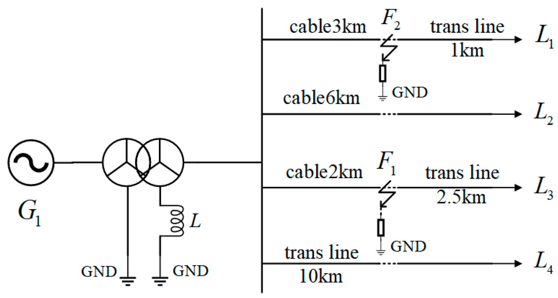
5.1. Testing Platform

The testing was conducted using the SL-03 single-phase grounding line selection device shown in Figure 8, which is from Beijing Hengtian Beidou Technology Co., Ltd., Beijing, China. The algorithm shown in Figure 7 was programmed into the device. Convert the test data into voltage and current signals via the platform, ultimately outputting the judgment result.

5.2. Simulation Verification

According to the previous analysis and calculation, k = 0.9, g = 50°, b₁ = 1.53, p₁ = −202.95°, q₁ = −111.6°, b₂ = 2.7, p₂ = 166.95°, q₂ = 289.74° can be obtained. The simulation data under different conditions are shown in

Table 3. Simulation inspection data table.

Fault Type	Resistance	Zero Sequence Voltage/Line Number	Phasor Variation (kV∠°/A∠°)	|ΔB| (kV)	Δφ(°)	Second Fault Line
Sequential grounding fault	R1 = 50 Ω R2 = 500 Ω	Zero sequence voltage	1.21∠87.83	-	-	Line 1
		1	8.64∠–94.34	33.53	−182.17
		2	0.61∠173.41	1.61	85.58
		3	8.61∠95.12	-	-
		4	0.03∠169.54	1.80	81.71
	R1 = 50 Ω R2 = 900 Ω	Zero sequence voltage	0.71∠88.04	-	-	Line 1
		1	5.00∠–91.55	19.64	−179.59
		2	0.47∠194.67	1.29	106.63
		3	4.99∠93.36	-	-
		4	0.02∠189.94	1.35	101.90
Reverse sequential grounding fault	R1 = 50 Ω R2 = 500 Ω	Zero sequence voltage	1.28∠27.62	-	-	Line 1
		1	8.61∠206.86	33.57	179.24
		2	0.59∠143.42	2.27	115.8
		3	8.47∠29.79	-	-
		4	0.04∠135.33	2.90	107.71
	R1 = 50 Ω R2 = 900 Ω	Zero sequence voltage	0.69∠34.27	-	-	Line 1
		1	4.97∠208.89	19.19	174.62
		2	0.37∠130.87	1.04	96.60
		3	5.11∠27.39	-	-
		4	0.03∠116.05	1.52	81.78

Note: The first grounding line has been selected according to the traveling wave method/transient method and is Line 3, which does not need to be included in the scope of successive fault inspection.

, and the results verify the correctness of the method.

The simulation results under interference conditions, as shown in

Table 4. Interference Simulation Test Table.

Fault Type	Fault Setting	Zero Sequence Voltage/Line Number	Phasor Variation (kV∠°/A∠°)	|ΔB| (kV)	Δφ(°)	Second Fault Line
Unstable single-phase grounding fault	R1 = 50 Ω R1n = 80 Ω	Zero sequence voltage	0.01∠−151.2	-	-	Do not accidentally start
		1	0.01∠120.6	-	-
		2	0.01∠120.6	-	-
		3	0.02∠−59.4	-	-
		4	0.01∠120.6	-	-
	R1 = 50 Ω R1n = 200 Ω	Zero sequence voltage	0.76∠113.54	-	-	Do not accidentally start
		1	0.27∠27.63	-	-
		2	0.26∠27.63	-	-
		3	0.20∠13.48	-	-
		4	0.26∠27.63	-	-
Successive fault with unstable grounding for the first time	Sequential grounding R1 = 50 Ω R1n = 200 Ω R2 = 500 Ω	Zero sequence voltage	4.17∠60.27	-	-	Line 1
		1	6.38∠247.35	28.04	187.08
		2	2.40∠154.75	5.94	94.48
		3	6.46∠55.21	-	-
		4	0.04∠155.34	4.62	95.07
	Reverse sequential grounding R1 = 50 Ω R1n = 200 Ω R2 = 500 Ω	Zero sequence voltage	3.75∠1.76	-	-	Line 1
		1	6.79∠−174.82	29.18	−176.58
		2	1.92∠95.32	5.38	93.56
		3	7.07∠−9.48	-	-
		4	0.03∠98.69	5.02	96.93

, demonstrate that this method exhibits strong anti-interference capabilities. For unstable single-phase grounding faults, the change in zero-sequence current on the faulted line is minimal and does not meet the criteria for initiating a successive fault. For successive faults resulting from unstable initial grounding faults, although multiple lines satisfy the criterion |ΔB_x| > b, the incorporation of the Δφ phase criterion still allows for the correct identification of the second faulty line. To further enhance the approach for this type of fault, an additional criterion can be considered: selecting the line with the maximum |ΔB| as the faulty line, thereby mitigating the interference effects caused by unstable faults.

Considering that there may be some errors in the zero sequence capacitance parameters obtained on site, it is assumed that there are errors in the zero-sequence capacitance of the faulty line 1, the faulty line 2, and the intact line. The sequential grounding faults of R₁ = 50 Ω and R₂ = 500 Ω are set for simulation testing. The results are shown in

Table 5. Simulation situation of parameter error interference.

Zero Sequence Capacitance Deviation of the Line	Zero Sequence Voltage/Line Number	Phasor Variation (kV∠°/A∠°)	|ΔB| (kV)	Δφ(°)	Second Fault Line
Line 1 +10%	Zero sequence voltage	1.22∠90.68	-	-	Line 1
	1	8.64∠−87.90	33.58	−178.58
	2	0.61∠188.28	1.56	82.40
	3	8.70∠87.63	-	-
	4	0.04∠197.08	1.31	106.4
Line 1 +30%	Zero sequence voltage	1.41∠80.24	-	-	Line 1
	1	8.71∠−94.31	34.03	−185.45
	2	0.61∠188.28	1.52	108.04
	3	8.95∠86.22	-	-
	4	0.04∠197.08	1.31	116.84
Line 2 +10%	Zero sequence voltage	1.27∠87.34	-	-	Line 1
	1	8.46∠−89.77	32.96	−177.11
	2	0.33∠159.75	1.56	72.41
	3	8.81∠87.74	-	-
	4	0.04∠188.94	1.26	101.60
Line 2 +30%	Zero sequence voltage	1.59∠75.03	-	-	Line 1
	1	8.49∠−89.77	33.34	−164.80
	2	0.79∠170.32	3.08	95.29
	3	9.18∠86.46	-	-
	4	0.05∠184.55	1.34	109.52
Line 3 +10%	Zero sequence voltage	1.21∠91.57	-	-	Line 1
	1	8.47∠−89.79	32.94	−181.36
	2	0.61∠188.28	1.57	96.71
	3	8.72∠87.64	-	-
	4	0.04∠187.39	1.26	95.82
Line 3 +30%	Zero sequence voltage	1.41∠80.24	-	-	Line 1
	1	8.46∠−89.77	33.08	−170.01
	2	0.67∠179.4	1.74	99.16
	3	8.86∠86.16	-	-
	4	0.04∠187.39	1.26	107.15

, indicating that this method has strong interference in this situation.

5.3. Field Data Verification

The field case is derived from an actual distribution network in Northwest China, which has a structure similar to that shown in Figure 2 and comprises a total of 24 outgoing lines. At 16:51:57 on a certain day, a grounding fault occurred on the line. The bus voltage was shown in Figure 9, and the A-phase voltage decreased. In addition, the amplitude of the zero-sequence current on line 12 was large and the phase was opposite to other lines. It was determined that line A was grounded. After a period of time, the line selection device activated and tripped the 12th switch of the line, but it was detected that the zero-sequence voltage still existed and the system grounding did not disappear.

At 17:00:42, switch 12 of the line was closed on site, and the bus voltage is shown in Figure 10. The voltage of phase C in Figure 10 is lower than that in Figure 9, indicating the presence of a phase C ground fault, which is a cross line grounding fault with different names. It is determined that the A phase of line 12 is grounded, causing an increase in the C phase voltage, which in turn leads to a breakdown grounding of the C phase of a certain line, resulting in a reverse sequence grounding fault. Subsequently, the switches of Line 12 and Line 3 were opened on site in sequence, and the zero-sequence voltage disappeared. The fault was resolved.

The calculation results are as follows: the zero-sequence voltage change ΔU₀ = 14.17 kV∠123.94°, and the zero sequence current change ΔI_{0_12} = 3.02 A∠8.82° of line 12 meet the starting criteria and are judged to be in reverse grounding condition. During the inspection of the remaining lines, the calculation results of Line 3 were |ΔB| = 53.88 kV and Δφ = 230.19°, which met the second fault line criterion under reverse grounding conditions, verifying the effectiveness of the algorithm proposed in this paper.

6. Conclusions

This article presents a comprehensive model and analysis of successive cross-line grounding faults with distinct phase characteristics in a neutral-point grounded distribution system equipped with arc suppression coils. The steady-state analytical expressions for the fault zero-sequence voltage and line zero-sequence current are derived using the phasor method. The study reveals significant differences in fault characteristics under various fault phase sequences, specifically identifying a unique differential relationship between the variations in zero-sequence current and zero-sequence voltage in the second faulted line. Based on the dynamic evolution of the fault process across different phase sequences, a novel detection method is proposed that not only accurately identifies the second faulted line but also determines the corresponding fault phase information. Both simulation and experimental data verify the effectiveness of the proposed algorithm, thereby providing a solid theoretical foundation for the design and development of fault detection, protection, and selection devices in distribution networks.

However, the method proposed in this article still exhibits certain limitations. It relies on data from the two steady states—before and after the transformation from a single-phase grounding fault to a two-point grounding fault—for selecting the fault line. Consequently, this method requires a relatively lengthy judgment process. Further research should explore adopting transient characteristic-based methods for successive faults.

References

1. Xu, B.; Li, T.; Xue, Y. Relaying Protection and Automation of Distribution Networks; China Electric Power Press: Beijing, China, 2017. [Google Scholar]
2. Liu, J.; Zhang, X.; Zhang, X. Treatment of a Single-phase Grounding Fault in a Small Current Grounding System to Prevent Fire in a Cable Trench. Power Syst. Prot. Control 2023, 51, 21–29. [Google Scholar]
3. Xue, Y.; Xie, Y.; Wen, F. A Review on Cascading Failures in Power System. Autom. Electr. Power Syst. 2013, 37, 1–9+40. [Google Scholar]
4. Wu, Z.; Cai, Y.; Zhang, J. Fault Analysis on Successive Fault of Multi-feeders Connected to the Same Bus in Resonant Grounding System. High Volt. Eng. 2017, 43, 2402–2409. [Google Scholar]
5. Wu, F.; Gu, Z. Analysis of the Cross-country Grounded Fault in the Low Current Grounded System. J. Shanghai Univ. Electr. Power 2020, 36, 524–528. [Google Scholar]
6. Ouyang, J.; Yu, X.; Zhou, Y. A Fault Line Selection Method for Two-Point Successive Grounding of Power Distribution Line. South. Power Syst. Technol. 2020, 14, 81–89. [Google Scholar]
7. Qi, Z.; Xue, Y.; Liu, J. Transient Characteristics of Cross-line Successive Grounding Faults and Applicability of Transient Line Selection Methods. Autom. Electr. Power Syst. 2023, 47, 156–165. [Google Scholar]
8. Zhang, Z.; Xue, Y.; Dong, L. Power Frequency Characteristics and Line Selection under Two Point Grounding Faults Occurring in Same Phase in Isolated Neutral System. Proc. CUS-EPSA 2022, 34, 9–16. [Google Scholar]
9. Lin, Z.; Liu, X.; Wang, Y. Centralized Protection for Low-resistance Grounding System Under Multi-point Grounding Fault. Proc. CSU-EPSA 2019, 31, 67–73. [Google Scholar]
10. Wang, X.; Zhang, F.; Gao, J. Cross-line same-phase successive fault detection method of flexible grounding system based on double vertical and horizontal criteria. Power Syst. Technol. 2025, 1–10. [Google Scholar]
11. Qi, Z.; Tian, J.; Xue, Y. Analysis of Power Frequency Electrical Quantity and Line Selection Applicability for Two-Point Grounding Faults Occurring on Different Phases in Isolated Neutral System. Trans. China Electrotech. Soc. 2023, 38, 3539–3551. [Google Scholar]
12. Xue, Y.; Qi, Z.; Cai, Z. Detection of Cross-line Different-phase Two-point Successive Grounding Fault Based on Change of Zero-sequence Admittance. Autom. Electr. Power Syst. 2023, 47, 174–183. [Google Scholar]
13. Wang, B.; Cui, X. Nonlinear Modeling and Analytical Analysis of Arc High Resistance Grounding Fault in Distribution Network with Neutral Grounding via Arc Suppression Coil. Proc. CSEE 2021, 41, 3864–3873. [Google Scholar]
14. Jiang, B.; Dong, X.; Shi, S. A Method of Single Phase to Ground Fault Feeder Selection Based on Single Phase Current Traveling Wave for Distribution Lines. Proc. CSEE 2014, 34, 6216–6227. [Google Scholar]
Figure 1. Cross line different-phase successive faults equivalent circuit.
Energies 18 02269 g001
Figure 2. Schematic diagram of simulation model.
Energies 18 02269 g002
Figure 3. Amplitude change of ΔI10: (a) When sequentially grounded; and (b) When reverse sequence grounded.
Energies 18 02269 g003
Figure 4. Phase change of ΔI10: (a) When sequentially grounded; and (b) When reverse sequence grounded.
Energies 18 02269 g004
Figure 5.B| change: (a) When sequentially grounded; and (b) When reverse sequence grounded.
Energies 18 02269 g005
Figure 6. Δφ change: (a) When sequentially grounded; and (b) When reverse sequence grounded.
Energies 18 02269 g006
Figure 7. Cross line different-phase successive faults line detection flowchart.
Energies 18 02269 g007
Figure 8. SL-03 single-phase grounding line selection device.
Energies 18 02269 g008
Figure 9. Bus voltage waveform at 16:51:57: (a) A-phase voltage; (b) B-phase voltage; (c) C-phase voltage; and (d) zero sequence voltage.
Energies 18 02269 g009aEnergies 18 02269 g009b
Figure 10. Bus voltage waveform at 17:00:42: (a) A-phase voltage; (b) B-phase voltage; (c) C-phase voltage; and (d) zero sequence voltage.
Energies 18 02269 g010