Fault Equivalence and Calculation Method for Distribution Networks Considering the Influence of Inverters on the Grid Side and the Distribution Network Side

Abstract

Due to the increasing availability of new energy sources, the adaptability of traditional fault analysis and calculation methods has declined when applied to distribution networks. The reason is that the traditional ideal voltage source model cannot accurately reflect the impact of new energy from the main grid side on distribution networks. Moreover, the existing calculation methods fail to consider the influence of new energy on both the grid side and the distribution network side simultaneously, resulting in relatively large calculation errors and inaccurate fault characteristics. To address the above problems, this paper first studies the control strategy and current output characteristics of typical inverter-based resources (IBR) and establishes an integrated source model for the grid side with a high proportion of IBRs during faults. The model employs a parallel connection of an ideal voltage source with series impedance and a voltage-controlled current source. A model parameter identification method is proposed, leveraging a genetic algorithm and utilizing the normal operating electrical quantities at the port. Then, a fault-equivalent model and an iterative method for calculating electrical quantities in distribution networks are proposed, based on the integrated grid-side model. The method takes into account both distributed generators (DGs) and IBRs on the grid side, using the voltage error at the point of common coupling (PCC) as the convergence criterion for the iterative calculation. The simulation results of PSCAD/EMTDC show that the proposed model and calculation method have high accuracy. The model precisely reflects the characteristics of reduced port voltage and limited current during faults on the grid side. The amplitude errors of the electrical quantities are within 1%, and the phase angle errors are within 4°.

1. Introduction

With a high proportion of new energy connected, power flow and fault characteristics of the distribution network change greatly [1,2,3]. The adaptability of the traditional power system fault analysis and calculation methods is also weakened, as they are based on synchronous generators [4,5]. The calculation accuracy of the fault electrical quantities is reduced, and the fault analysis, protection setting adjustments, and calibration of electrical equipment based on the traditional methods are all greatly affected [6].

As far as the distribution network side is concerned, the distributed generators (DGs) are mostly connected to the distribution network through inverters, and their impact during faults mainly depends on the structure and control characteristics [7]. In recent years, to improve the fault calculation accuracy and clarify the fault characteristics of distribution networks, many studies have analyzed the correlation characteristics of the port voltage and port current for networks with IBRs connected, and established fault-equivalent models of IBRs. The models of voltage-controlled current sources and voltage sources in series with a variable impedance are mostly used. The transient voltage of the source under each time step is approximately solved by the numerical method, but the fault ride-through strategy is not applied to DGs. Reference [8] modeled the DG as a constant voltage in series with a constant impedance to calculate the short-circuit current in the distribution network. However, achieving a high level of calculation accuracy is challenging. References [9,10,11] found that inverter-based DGs output different current values depending on the voltage level at the point of common coupling (PCC) before and after the fault, and then, based on the substitution theorem, voltage-controlled current sources are used to replace the DG under different conditions. The short-circuit currents in distribution networks are calculated through global iterations, with the method exhibiting high accuracy. In [12], the sequence component voltage-controlled current source model of the DG was established, combining the sequence current control of the DG and reactive power support during faults. The fault current and power of the inverter-based DG were calculated by a composite sequence network model of the distribution network. In [13], a graph convolutional neural network-based short-circuit current calculation method was proposed to improve the calculation speed and accuracy during the connection of multiple DGs. Additionally, a droop-controlled DG-connected distribution network was analyzed in [14] through the transfer function of the inverter control loop, while a very simple network was modeled for simplicity in the analysis.

The above studies mainly consider the effects of IBRs on the distribution network side. In fact, under the scenario of high new energy penetration, a large number of IBRs are also connected to the main grid side of the distribution network, affecting the fault characteristics of the distribution network containing DGs. In the above studies, the main grid side of the distribution network is only modeled as a synchronous generator, meaning that the impacts of the IBRs are not considered.

Regarding the main grid equivalence incorporating new energy resources, references [15,16] utilized Thevenin’s or Norton’s theorem as the foundational approach. Reference [15] corrected the impedance-based grid model using the equivalent potential method to reflect the voltage support role of the external grid containing new energy. Reference [16] analyzed the impact of high new energy penetration on the calculation of short-circuit current and grid equivalence parameters of the grid through multi-port Thevenin equivalence; however, its equivalence demands highly detailed network parameters. These studies mainly focus on the main grid containing new energy but fail to study its impact on the distribution network side. The key findings and limitations of the mentioned references are listed in

Table 1. Comparison of fault equivalence and analysis for distribution networks and the main grid.

Reference	DG Model	Grid-Side Model	Key Findings	Limitations
[8]	Constant voltage in series with a constant impedance	New energy sources are not mentioned	Calculate the fault current in the active distribution network; the fault calculation error is less than 5%	The impacts of grid-side IBRs are not considered; the calculation error is relatively large
[9]	Voltage-controlled current sources	Ideal current source in parallel with admittance	Improve the fault calculation accuracy compared to the case where DGs are not considered	The impacts of grid-side IBRs are not considered
[10]	Voltage-controlled current sources	Ideal voltage source in series with impedance	Propose a fault ride-through control strategy to enhance the efficiency of DGs and calculate the fault electrical quantities based on this strategy	The impacts of grid-side IBRs are not considered
[11]	Voltage source in series with an impedance	New energy sources are not mentioned	Calculate the fault electrical quantities by forming a new admittance matrix	The impacts of grid-side IBRs are not considered
[12]	Sequence component voltage-controlled current source	Ideal voltage source in series with impedance	Propose a fault calculation method for asymmetrical faults based on the composite sequence network	The impacts of grid-side IBRs are not considered; injection of the negative-component current for IBRs is not common
[13]	No physical model is available	No physical model is available	Propose a graph convolutional neural network-based calculation method to improve accuracy and computational speed	The impacts of grid-side IBRs are not considered; there is a lack of physical models as the theoretical basis
[14]	Voltage-controlled current sources (PQ control) and voltage source (VF control)	Ideal voltage source in series with impedance	Analyze the fault currents under different IBR control strategies	The impacts of grid-side IBRs are not considered
[15]	DG is not taken into consideration	Ideal voltage source in series with impedance	Use the equivalent potential method to reflect the voltage support role of the external grid containing new energy	The impacts of distribution network-side IBRs are not considered; the characteristics of distribution network are not analyzed
[16]	Ideal current source in parallel with admittance	No specific explanation is available, but it can refer to the DG model	Analyze the impact of high new energy penetration on the calculation of short-circuit currents	The impacts of the grid-side IBR on the distribution network are not considered

.

In general, the existing references fail to consider the effects of IBRs on both the main grid side and the distribution network side, and there is a lack of research on fault calculation for such distribution networks. To solve this problem, this paper proposes a fault equivalence and calculation method for distribution networks that takes into account the effects of both grid-side and distribution-network-side IBRs, with the following contributions:

(1)

An integrated grid-side source model and a parameter identification method for distribution network faults are proposed, both of which can accurately reflect the impact of the IBRs on the grid side of the distribution network containing DGs. The key parameters are identified based on the port electrical quantities, using the genetic algorithm.

(2)

A fault calculation method that takes into account the impact of IBRs on the grid side and distribution network side is proposed which can accurately calculate the electrical quantities of the distribution network and provide a reliable basis for fault characteristic analysis and protection settings.

The rest of the paper is organized as follows. Section 2 analyzes the typical control strategies and current features of IBRs. Section 3 proposes an equivalent model of the main grid side containing a high proportion of IBRs for distribution network faults. Section 4 proposes a fault calculation method for distribution networks with IBRs on both the grid and the distribution network sides. Then, the proposed fault-equivalent model and calculation method are verified in Section 5 by PSCAD/EMTDC simulation, followed by the conclusions.

2. Typical Control Strategies and Current Features of IBRs

The control strategies of existing inverters are mainly divided into two types: grid-following (GFL) control and grid-forming (GFM) control. The former follows the alternating current (AC) voltage established by the external system to provide power to the grid, and has the advantages of flexible settings, well-developed technology, and more. It is the most widely used strategy for IBRs [17]. Therefore, this paper mainly focuses on the scenarios in which the high proportion of GFL inverters are connected to the grid side and distribution network side.

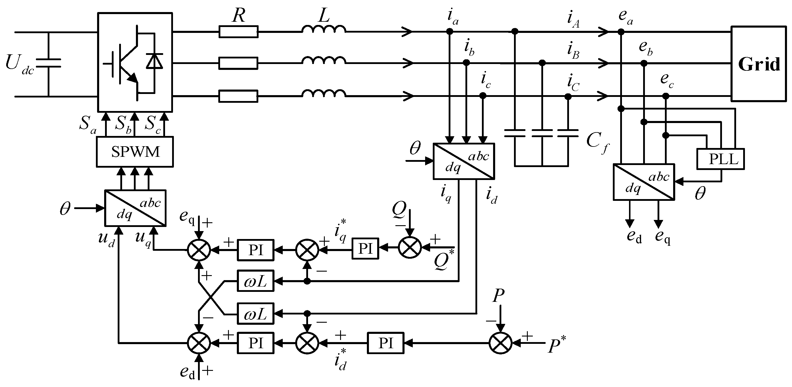
2.1. Control Strategy During Normal Operation

The control structure of the three-phase grid-connected inverter is shown in Figure 1. Double-loop control is one of the most widely used methods and is divided into an inner-loop and an outer-loop control. The outer loop is used to meet different control objectives and outputs reference signals to the inner loop, which has a slower dynamic response speed and generally adopts constant power control (PQ control) [18]. The inner loop is set for fine tuning, improving the quality of power output from the inverter, and its dynamic response speed is faster. The inner-loop control under the dq rotating coordinate system is a common strategy.

In Figure 1, U_dc is the voltage on the DC side; R and L are the resistance and inductance, respectively, from the inverter to the grid; C_f is the filter capacitor; e_d and e_q are the components of the PCC voltage e_a, e_b, and e_c in the dq coordinate system, respectively; i_d and i_q are the components of the output current i_a, i_b, and i_c in the dq coordinate system, respectively; $i_d^{*}$ and $i_{\mathrm{q}}^{*}$ are the reference values of i_d and i_q, respectively; P and Q are the instantaneous active power and reactive power, respectively; P* and Q* are the reference values; θ is the angle output of the phase-locked loop (PLL); S_a, S_b, and S_c are the switching functions of each phase for grid-connected inverter modulation.

PQ control aims to ensure that the active and reactive power outputs of the DG match the reference values. This means that, when the frequency and voltage of the AC system connected to the inverter change within the permitted range, the active and reactive power of the DG remain unchanged [19]. The essence of PQ control is to decouple active power and reactive power in the dq coordinate system and control them separately. Through the dq transformation, the AC quantities in the three-phase stationary coordinate system can be transformed into DC quantities in the two-phase dq rotating coordinate system in order to track the reference values. PQ control based on grid voltage vector orientation is a commonly used control method, and the expressions for active and reactive power are as follows [20]:

$$\left\{\begin{array}{l}p=1.5e_{\mathrm{d}}{i}_{\mathrm{d}}\\ q=1.5e_{\mathrm{d}}{i}_{\mathrm{q}}\end{array}\right.,$$

(1)

When the grid voltage is unchanged, the control of $i_{\mathrm{d}},i_{\mathrm{q}}$ can realize the independent control of p and q, so the outer-loop control can be achieved by the PI control section.

The inner-loop control equations can be obtained according to the physical model of the inverter and can be expressed as follows [21]:

$$\left\{\begin{array}{l}{u}_{\mathrm{d}}=(K_{\mathrm{P}}+{\displaystyle \frac{K_{\mathrm{I}}}{s}})(i_{\mathrm{d}}^{*}-i_{\mathrm{d}})-{\omega }_{0}L{i}_{\mathrm{q}}+e_{\mathrm{d}}\\ u_{\mathrm{q}}=(K_{\mathrm{P}}+{\displaystyle \frac{K_{\mathrm{I}}}{s}})(i_{\mathrm{q}}^{*}-i_{\mathrm{q}})+{\omega }_{0}L{i}_{\mathrm{q}}+e_{\mathrm{q}}\end{array}\right.$$

(2)

where K_P and K_I are the proportional and integral regulation gains, respectively, of the inner loop of the current control.

2.2. Control Strategy for Low-Voltage Ride-Through Periods

To prevent the large-scale disconnection of IBRs during faults, it is usually required to ensure that the IBRs remain connected to the grid for a certain period when the voltage is lower than the rated value. Then, the IBRs can provide support for the grid when they enter the low-voltage ride-through period [22].

When the voltage at the PCC is normal, IBRs only output active power to achieve maximum utilization of energy, based on the active power reference value of the outer loop. During fault conditions, when the voltage at the PCC falls below 0.9 times the rated voltage, the IBRs enter the low-voltage ride-through period. The outer loop of the IBRs is disconnected at this point, and the reference values for the active and reactive currents are provided directly to the inner loop. Meanwhile, the current provided by the IBRs is typically referenced to the positive-sequence voltage component to improve the output characteristics of the IBRs during asymmetrical faults and suppress the influence of the negative-sequence component. The IBRs generally follow the principle that reactive power is preferentially output to support the voltage, and the remaining capacity can be used for active power. The reactive and active reference currents can be expressed as follows [21,23,24].

$$i_{\mathrm{q}}^{*}=\left\{\begin{array}{l}0,\hspace{1em}\hspace{1em}\hspace{1em}\hspace{1em}\hspace{1em}\hspace{1em}{U}_{\mathrm{PCC}}^{+}>0.9\\ k_{\mathrm{q}}(1-U_{\mathrm{PCC}}^{+}) U_{\mathrm{L}}<U_{\mathrm{PCC}}^{+}<0.9\\ I_{\max },\hspace{1em}\hspace{1em}\hspace{1em}\hspace{1em}\hspace{1em}{U}_{\mathrm{PCC}}^{+}<U_{\mathrm{L}}\end{array}\right.$$

(3)

$$i_{\mathrm{d}}^{*}=\min \{I_{\mathrm{dref}},\sqrt{I_{\max }^2-{(i_{\mathrm{q}}^{*})}^2}\}$$

(4)

where $U_{\mathrm{P}\mathrm{C}\mathrm{C}}^{+}$ is the nominal value of the positive-sequence voltage at the PCC, and k_q is the proportionality coefficient of the reactive current, with a range of 1.5–6. U_L is the boundary where the IBRs cannot provide enough reactive current, as determined by k_q times the voltage drop required by the equation, once the current limitation is reached. I_max is the maximum allowable output current value, with a range of 1.2–2. The parameter k_q is taken to be 2, and the maximum current value is taken to be 1.5, referring to the German grid connection standard. IBRs typically use the positive-sequence voltage at the PCC as a reference to suppress the output of negative-sequence currents, thereby preventing potential inverter tripping that could be caused by them. Therefore, under different fault conditions, the inverter only outputs positive-sequence steady-state current [23].

Based on the different degree of voltage drop, the IBRs can be divided into three cases in the low-voltage ride-through state: (1) providing the reactive current according to the ride-through requirement and the active reference value; (2) providing the reactive current according to the ride-through requirement and part of the active reference current; and (3) only providing reactive current according to the upper current limit of the IBRs. The boundary between state (1) and (2) is called the control boundary. The PCC voltage U_X is the voltage at the control boundary, and it can be solved by Equation (5). U_L is the boundary voltage between (2) and (3).

$${[2(1-{\displaystyle \frac{U_{\mathrm{x}}}{U_{\mathrm{N}}}})I_{\mathrm{N}}]}^2+{({\displaystyle \frac{P_{\mathrm{ref}}}{1.5U_{\mathrm{x}}}})}^2={(1.5I_{\mathrm{N}})}^2.$$

(5)

Its per unit value form is as follows:

$${[2(1-U_{\mathrm{x}})]}^2+{({\displaystyle \frac{1}{1.5U_{\mathrm{x}}}})}^2={1.5}^2.$$

(6)

From the above equation, U_X = 0.719 p.u. can be obtained, alongside U_L = 0.25 p.u. Then, the IBR output currents under different voltage drops are as follows.

$$I_{\mathrm{IBR}}=\left\{\begin{array}{l}{\displaystyle \frac{1}{U_{\mathrm{PCC}}^{+}}}-\mathrm{j}2(1-U_{\mathrm{PCC}}^{+})\hspace{1em}\hspace{1em} 0.719 \mathrm{p}.\mathrm{u}.\le U_{\mathrm{PCC}}^{+}\le 0.9 \mathrm{p}.\mathrm{u}.\\ \sqrt{{(1.5)}^2-{[2(1-U_{\mathrm{PCC}}^{+})]}^2}-\mathrm{j}2(1-U_{\mathrm{PCC}}^{+}) 0.25 \mathrm{p}.\mathrm{u}.\le U_{PCC}^{+}\le 0.719 \mathrm{p}.\mathrm{u}.\\ \mathrm{j}1.5 \hspace{1em}\hspace{1em}\hspace{1em}\hspace{1em}\hspace{1em}\hspace{1em}\hspace{1em}\hspace{1em}\hspace{1em}\hspace{1em}\hspace{1em} U_{PCC}^{+}\le 0.25 \mathrm{p}.\mathrm{u}.\end{array}\right.$$

(7)

It should be noted that the phase angle of the current phasor is relative to the phase angle of the PCC voltage, rather than to the absolute value.

3. Equivalent Model of the Grid Side Containing a High Proportion of IBRs

In the traditional models of faulted distribution networks, the grid side is typically represented as a voltage source in series with impedance, focusing solely on the fault characteristics of conventional synchronous generators. However, as IBRs become increasingly integrated into the grid, their inherently strong nonlinear output characteristics significantly alter the fault characteristics at the port. For the distribution network, this change leads to inaccuracies in calculating electrical quantities and hampers the effective analysis of fault features.

Therefore, Section 3 proposes an integrated source model for the grid side. It uses a simplified yet comprehensive approach to accurately reflect the nonlinear characteristics of the grid side, which includes multiple IBRs as well as multiple traditional generator sources, as shown in Figure 2. Furthermore, the key parameters of the model can be identified by the voltage and the current at the grid-side port, offering convenience and practicality. Figure 3 illustrates a comparison between the traditional grid-side source model and the proposed integrated source model.

3.1. Integrated Source Model

The IBRs output three symmetrical currents under normal or fault conditions, and the current amplitude and phase angle depend on the control strategy of the IBRs, such a strategy being mainly affected by the voltage at the PCC. Overall, the IBRs can be modeled as voltage-controlled current sources, which are controlled by the PCC voltage [25]. For multiple IBRs with the same control strategy, their output currents exhibit the same nonlinear characteristics with respect to the PCC voltage. Thus, they can be aggregated into one IBR and then equated with a single voltage-controlled current source. For IBRs with different control strategies, their output currents and PCC voltages exhibit different nonlinear relationships, so it is not possible to directly aggregate them. In this study, the IBRs on the grid side all adopt the same control strategy, so they are equated with a single voltage-controlled current source. As for the IBRs and synchronous generator sources on the grid side, there is a significant difference between their output characteristics. Therefore, this paper models the two types of power sources separately and connects them in parallel. Under the fault conditions in the distribution network, the grid-side integrated source equivalence model is then proposed, based on the output characteristics of the two types of sources and the circuit theorem, as shown in Figure 3.

3.2. Parameter Identification Method

There are three parameters in the integrated source model, namely the source voltage, E_S, the impedance, Z_S, and the output current of the IBRs during normal operation, I_NEW. Once I_NEW is identified, the current of the IBRs during faults can be obtained in combination with Equation (7). The magnitude of E_S is an empirical value based on the practical operation state of the grid; Z_S and I_NEW are not easily obtained from experience, and an identification method is then proposed for the two parameters. The essence of identification is to find the optimal set of parameters for the integrated source model that best matches the output characteristics of the main grid. In this paper, identification of Z_S and I_NEW is achieved, provided that only the port voltage U and current I at the grid side during normal operation are known.

Parameter identification is essentially an optimization process. Common optimization algorithms include sequential quadratic programming (SQP) [26], simulated annealing (SA) [27], genetic algorithm (GA), and more. The SQP algorithm converges quickly and has strong local search capabilities, but it is sensitive to the initial point and struggles with discontinuous and nonlinear problems. SA has strong global search capabilities and can escape local optima, making it suitable for both discrete and continuous optimization problems. However, it converges slowly, requires a long computational time, and is difficult to tune. It also has some dependence on the initial point. The GA is a type of stochastic global search optimization algorithm which searches a group of candidate individuals without specific search directions. It directly takes the value of the fitness function as the evaluation index, an approach that is suitable for dealing with complex nonlinear and discontinuous optimization problems, and exhibits good convergence and anti-noise ability. Moreover, it does not require gradient information, is applicable to non-differentiable functions, and is independent of the initial point. The convergence speed of GA is moderate. Therefore, considering the strong capability of GA in handling complex problems and its adaptability, this paper employs the GA for parameter identification.

The specific process is as follows. First, initialize the parameter population to be identified and encode the initial population. Then, repeat the four operations of calculating the fitness function, selection, crossover, and mutation to update the population and find the optimal solution. The calculation will be terminated if the end conditions are met or the number of solutions reaches the maximum. Take the optimal individual in the population and decode the target value. The process is shown in Figure 4, and the detailed steps are as follows.

Step 1: Once the range of the parameters to be recognized is specified, initialize the population. Searching within the specified range can greatly reduce the amount of calculation and improve the recognition accuracy. Combined with the practical condition, set the maximum of the parameter to be recognized, Z_S, as Z_max, the minimum of Z_S as Z_min, the maximum of I_NEW as I_NEW.max, and the minimum of I_NEW as I_NEW.min. Experientially, 0 Ω ≤ Z_S ≤ 100 Ω; 0 kA ≤ I_NEW ≤ 0.5 kA. Set the size of the population to 100, a value that ensures the diversity of the individuals in the population and does not make the solving time excessively long. The initial population is obtained by taking 100 random numbers within the specified range of the parameters.

Step 2: Encode the initial population in binary form. Individuals in the initial population are decimal numbers, with which it is not easy to perform crossover and mutation operations. Therefore, it is necessary to encode the initial population and transform the expression form of the initial population for subsequent operations. The conversion relationship between the binary coding results and the values of the parameters to be recognized is shown in Equation (8). From Equation (8), it can be seen that the greater the number of coding bits, the higher the numerical accuracy of the parameters and the more accurate the correspondence between the binary code and the parameters. However, more coding bits will increase the amount of computation. Thus, the number of coding bits is selected with the coding accuracy and computational speed considered simultaneously.

$$\eta ={\displaystyle \frac{\epsilon -{\epsilon }_{\min }}{{\epsilon }_{\max }-{\epsilon }_{\min }}}(2^n-1)$$

(8)

where ${\epsilon }_{\max }$ and ${\epsilon }_{\min }$ are the maximum and minimum values, respectively, of the parameters; ε is the value of the parameters; and n is the number of binary encoding bits.

Step 3: Calculate the fitness function. The fitness function is an evaluation index of the individual advantages and disadvantages in the population. Since two electrical quantities are known, including the grid-side bus voltage phasor and the current phasor during normal operation of the distribution network, the output current I of the grid side can be calculated according to Ohm’s law and Kirchhoff’s current law (KCL). Calculate the difference between the calculated and measured values of the current, and then take the modulus of the difference as the fitness function, as shown in Equation (9). When substituting the individuals in the population into Equation (9) yields a smaller value, it indicates that the result is closer to the target value.

$$value=\left|{\displaystyle \frac{E_S\angle {\theta }_{\mathrm{E}}-U\angle {\theta }_{\mathrm{U}}}{Z_S\angle {\theta }_{\mathrm{z}}}}+I_{\mathrm{NEW}}\angle {\theta }_{\mathrm{U}}-I\angle {\theta }_{\mathrm{I}}\right|$$

(9)

where θ_E and θ_Z are the phase angle of E_S and the phase angle of the internal impedance Z_S in the synchronous generator source equivalent model, respectively. Empirical values are used for these phase angles. θ_U and θ_I are the measured phase angles of the port voltage U and the port current I, respectively.

Step 4: Selection, crossover, and mutation operations are performed on the population. First, the roulette algorithm is used to select individuals from the population. According to the order of the individuals in the population, the reciprocal of the fitness function value of each individual is divided by the sum of the reciprocals of the fitness function values of all individuals to obtain the fitness function probability for each individual. The cumulative probability for each individual is then calculated by summing the fitness function probabilities of all preceding individuals. Select an individual whose cumulative probability is greater than a randomly chosen number between 0 and 1. Repeat this operation 100 times. Then, the selected individuals are paired sequentially, with each pair corresponding to a randomly chosen number between 0 and 1. If the random number is greater than the crossover rate, a crossover is performed on the pair of individuals; otherwise, no operation is performed. Finally, for each individual, a random number between 0 and 1 is assigned. If the random number is greater than the mutation rate, a mutation is performed on the individual; otherwise, no operation is performed.

Step 5: Judge whether to terminate the operation or not. At the beginning of the algorithm, the maximum number of iterations is preset to 200. If the optimal solution that meets the conditions is found before the number of iterations reaches 200, the operation is terminated, and the optimal value is output. The termination condition is that the value of the fitness function in Equation (9) is lower than v_set. The accuracy of parameter identification is high when the error v_set is low. If the optimal solution is not found when the number of iterations reaches 200, the operation is terminated, and the optimal solution in the existing results is output. One option is to rerun the computation program or to initiate a new round of computations after adjusting the parameters of the genetic algorithm, a process that does not lead to a long computation time but rather ensures a certain degree of convergence.

Step 6: Decode the results. Substitute the output of the fifth step into Equation (8) for the inverse operation to obtain the decimal optimal solution.

4. Fault Calculation Method for Distribution Networks with IBRs on Both Grid and Distribution Sides

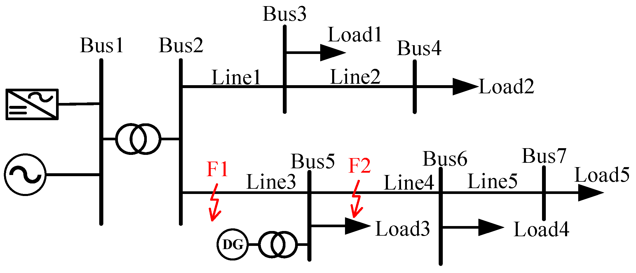
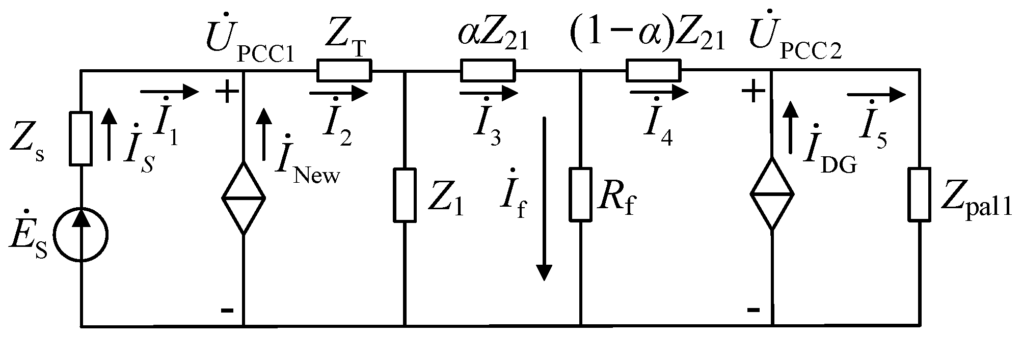
4.1. Fault-Equivalent Model of Distribution Networks

Under the condition of coexistence of synchronous generator sources and a high proportion of IBRs on the grid side, the distribution network is shown in Figure 5, in which the main grid-side source is modeled as the proposed integrated source.

For the distribution network shown in Figure 5, when the DG on the distribution network side is a GFL-type IBR, the fault equivalence model during three-phase faults at F1 and F2 is shown in Figure 6. Z_T is the equivalent impedance of the step-down transformer; Z₁ is the equivalent impedance of the entire feeder line where line 1 is located; Z₂₁ is the equivalent impedance of line 3; Z₂₂ is the equivalent impedance of line 4; Z₂₃ is the equivalent impedance of line 5; Z_L21 is the equivalent impedance of load 3; Z_L22 is the equivalent impedance of load 4; Z_L23 is the equivalent impedance of load 5; Z_pal1 is the equivalent impedance of the circuit on the right side of the blue dotted line; and Z_pal2 is the equivalent impedance of the part of the circuit to the right of the green dotted line. The terms α and β are constants, and their range is (0, 1). ${\dot{I}}_{\mathrm{N}\mathrm{e}\mathrm{w}}$ is the IBR output current of the main grid side during faults, while ${\dot{I}}_{\mathrm{D}\mathrm{G}}$ is the output current of the DG in the distribution network. The distribution network in Figure 6 is used to study the fault analysis method under the condition of a high proportion of new energy.

When a three-phase short-circuit fault occurs at F1, the simplified equivalent circuit is shown in Figure 7. R_f is the fault resistance, and ${\dot{I}}_{\mathrm{f}}$ is the current flowing through the fault point.

To solve the electrical quantities in the distribution network, the equations can be written as follows, based on Ohm’s law and KCL.

$$\left\{\begin{array}{l}{\dot{E}}_{\mathrm{S}}=Z_{\mathrm{S}}{\dot{I}}_1+{\dot{U}}_{\mathrm{PCC}1}\hfill \\ {\dot{U}}_{\mathrm{PCC}1}=(Z_{\mathrm{T}}+Z_1){\dot{I}}_2-Z_1{\dot{I}}_3\hfill \\ 0=(Z_1+R_{\mathrm{f}}+\alpha Z_{21}){\dot{I}}_3-Z_1{\dot{I}}_2-R_{\mathrm{f}}{\dot{I}}_4\hfill \\ -{\dot{U}}_{\mathrm{PCC}2}=[R_{\mathrm{f}}+(1-\alpha )Z_{21}]{\dot{I}}_4-R_{\mathrm{f}}{\dot{I}}_3\hfill \\ {\dot{U}}_{\mathrm{PCC}2}=Z_{\mathrm{pal}1}{\dot{I}}_5\hfill \\ {\dot{I}}_{\mathrm{New}}={\dot{I}}_2-{\dot{I}}_1\hfill \\ {\dot{I}}_{\mathrm{DG}}={\dot{I}}_5-{\dot{I}}_4\hfill \end{array}\right..$$

(10)

Key quantities can be solved according to Equation (11).

$$\left\{\begin{array}{l}{\dot{U}}_{\mathrm{PCC}1}={\displaystyle \frac{1}{B}}[(Z_1^2{Z}_{13}{R}_f+A{Z}_{l1}{R}_f)({\displaystyle \frac{{\dot{E}}_{\mathrm{S}}}{Z_{\mathrm{S}}}}+{\dot{I}}_{\mathrm{New}})+(Z_1{Z}_{l2}{Z}_{l3}{Z}_{\mathrm{pal}1}-A{Z}_1{Z}_{\mathrm{pal}1}){\dot{I}}_{DG}]\\ {\dot{I}}_4={\displaystyle \frac{1}{A}}[Z_{l2}{Z}_{\mathrm{pal}1}{\dot{I}}_{DG}-R_f(Z_1{\dot{I}}_{\mathrm{New}}+{\displaystyle \frac{Z_1{\dot{E}}_{\mathrm{S}}}{Z_{\mathrm{S}}}})+{\displaystyle \frac{R_f{Z}_1}{Z_{\mathrm{S}}}}{\dot{U}}_{\mathrm{PCC}1}]\\ {\dot{U}}_{\mathrm{PCC}2}=Z_{\mathrm{pal}1}({\dot{I}}_{DG}+{\dot{I}}_4)\end{array}\right.$$

(11)

When a three-phase short-circuit fault occurs at F2, the equivalent circuit can be simplified as shown in Figure 8. Similarly, the equation can be written as follows, and then each electrical quantity in the distribution network can be solved in the same way.

$$\left\{\begin{array}{l}{\dot{E}}_{\mathrm{S}}=Z_{\mathrm{S}}{\dot{I}}_1+{\dot{U}}_{\mathrm{PCC}1}\hfill \\ {\dot{U}}_{\mathrm{PCC}1}=(Z_{\mathrm{T}}+Z_1){\dot{I}}_2-Z_1{\dot{I}}_3\hfill \\ -{\dot{U}}_{\mathrm{PCC}2}=(Z_1+Z_{21}){\dot{I}}_3-Z_1{\dot{I}}_2\hfill \\ {\dot{U}}_{\mathrm{PCC}2}=Z_{\mathrm{L}21}{\dot{I}}_4-Z_{\mathrm{L}21}{\dot{I}}_5\hfill \\ 0=(Z_{\mathrm{L}21}+\alpha Z_{22}+R_{\mathrm{f}}){\dot{I}}_5-Z_{\mathrm{L}21}{\dot{I}}_4-R_{\mathrm{f}}{\dot{I}}_6\hfill \\ 0=[R_{\mathrm{f}}+(1-\alpha )Z_{22}+Z_{\mathrm{pal}2}]{\dot{I}}_6-R_{\mathrm{f}}{\dot{I}}_5\hfill \\ {\dot{I}}_{\mathrm{New}}={\dot{I}}_2-{\dot{I}}_1\hfill \\ {\dot{I}}_{\mathrm{DG}}={\dot{I}}_4-{\dot{I}}_3\hfill \end{array}\right.$$

(12)

4.2. Fault Calculation Process for Distribution Networks

From the equations above, it is evident that the output currents of the IBRs on the grid side and the distribution network side are unknown. Their magnitudes and phase angles are controlled by the PCC voltage; therefore, it is not possible to directly obtain the electrical quantities in the distribution network through the above expressions. In order to perform the fault calculation, first, disconnect the IBRs on the grid side and distribution network side from the network. Then, set the following values, ${\dot{I}}_{\mathrm{N}\mathrm{e}\mathrm{w}}=0$ and ${\dot{I}}_{\mathrm{DG}}=0$, to obtain the initial values of the PCC voltage, according to Equation (11) or Equation (12). As shown in Equation (7), the output current of the IBRs can be further determined according to the two initial PCC voltages on the grid side and distribution network side. The current amplitude can be directly calculated, and the phase angle difference between the current phasor and the voltage phasor is equal to the phase angle of I_IBR in Equation (7). Then, calculate the phase angles of the IBRs, and determine ${\dot{I}}_{\mathrm{N}\mathrm{e}\mathrm{w}}$ and ${\dot{I}}_{\mathrm{DG}}$. Substitute them into Equations (11) and (12) to obtain the electrical quantities, including ${\dot{U}}_{\mathrm{P}\mathrm{C}\mathrm{C}1}$ and ${\dot{U}}_{\mathrm{P}\mathrm{C}\mathrm{C}2}$. Thus, the differences between the new and previous PCC voltages can be calculated and denoted as ε₁ and ε₂, respectively. The terms ε₁ and ε₂ represent the differences in U_PCC1 and U_PCC2, respectively. Repeat the process above. When the iterative calculation error is less than the error threshold ε_set, the process terminates. At the end of the iteration, the accuracy of the fault calculation meets the requirements. The fault calculation process is shown in Figure 9.

5. Simulation and Verification

The simulation model of the 10 kV distribution network shown in Figure 2 is established in PSCAD/EMTDC. Take the rated voltage on the grid side as 110 kV and take the rated voltage of the distribution network side as 10 kV. The voltage of the synchronous generator source is 115 kV. The type of step-down transformer is Yd11. The line parameter for the per unit length is 0.125 + j0.095 Ω/km; the lengths of line 1, line 2, line 3, line 4, and line 5 are 2 km, 4 km, 5 km, 4.8 km, and 3 km, respectively. The rated capacities of load 1, load 2, load 3, load 4, and load 5 are 2.0 + j0.5 MVA, 1.9 + j0.624 MVA, 1.5 + j0.3 MVA, 1.9 + j0.624 MVA, and 1.9 + j0.624 MVA, respectively. The IBRs use the PQ control strategy during normal operation, and the low-voltage ride-through control strategy during faults. A 2 MW DG is connected to the distribution network at bus 5, using the same control strategies.

The grid-side detailed simulation model containing multiple synchronous machines and IBRs is used to output accurate measured voltage and current at the port. The parameters of the simplified integrated source model are then identified based on the voltage and current.

5.1. Verification of Integrated Source Model for the Grid Side

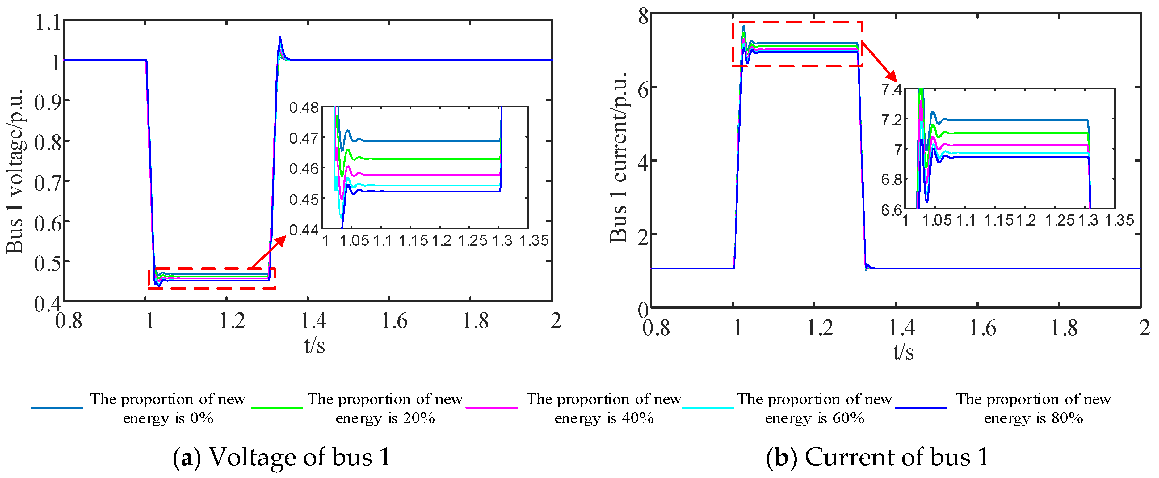
5.1.1. Impact of the Grid-Side IBR on the Fault Characteristics of Distribution Networks

Three-phase fault cases of F3 are studied to verify the proposed source model. The faults occur at t = 1.0 s and are cleared at t = 1.3 s. The fault resistance is 0.5 Ω. On the basis of maintaining the voltage of bus 1 at 110 kV, the output power of the IBRs is adjusted to simulate different cases for grid-side sources with varying levels of IBR penetration. The impact of the grid-side IBRs on the fault characteristics of the distribution network is analyzed by comparing the fault currents and fault voltages at bus 1 on the grid side of the distribution network. Penetration of the grid-side IBRs is set to 0, 20.0%, 40.0%, 60.0%, and 80.0%, respectively. The voltages and currents of bus 1 are shown in Figure 10.

As can be seen from the figure above, during faults in the distribution network, when the penetration increases from 0 to 80.0%, the voltage of bus 1 reduces from 0.469 p.u. to 0.452 p.u., and the fault current flowing through bus 1 decreases from 7.192 p.u. to 6.943 p.u. It is clear that the grid-side bus voltage and fault current decrease due to the limitations of the output reactive power and maximum output current of the IBRs. The high proportion of IBRs on the grid side of the distribution network causes the fault characteristics of the distribution network to change.

5.1.2. Verification of the Parameter Identification Method

The rated capacity of the IBRs is set to 5 MW, 10 MW, 15 MW, and 20 MW, and the proportion of new energy is 20.0%, 40.0%, 60.0%, and 80.0% respectively. Based on the voltage and current phasors at bus 1 during normal operation under different proportions of IBRs, the parameters of the integrated source model are identified by the proposed genetic algorithm process. The crossover rate is set to 0.8. The simulation results are listed in

Table 2. Parameter identification results of the integrated source model.

Percentage of New Energy/%	Parameter	Set Value/p.u.	Identified Value/p.u.	Error/%
20	z	0.092	0.091	1.087
	IPW	0.200	0.196	2.000
40	z	0.097	0.097	1.031
	IPW	0.400	0.395	1.250
60	z	0.104	0.104	1.818
	IPW	0.600	0.595	0.833
20	z	0.110	0.108	1.818
	IPW	0.800	0.797	0.375

.

From the table above, it can be seen that the parameters of the integrated source model can be identified effectively through the proposed method. The method has good feasibility.

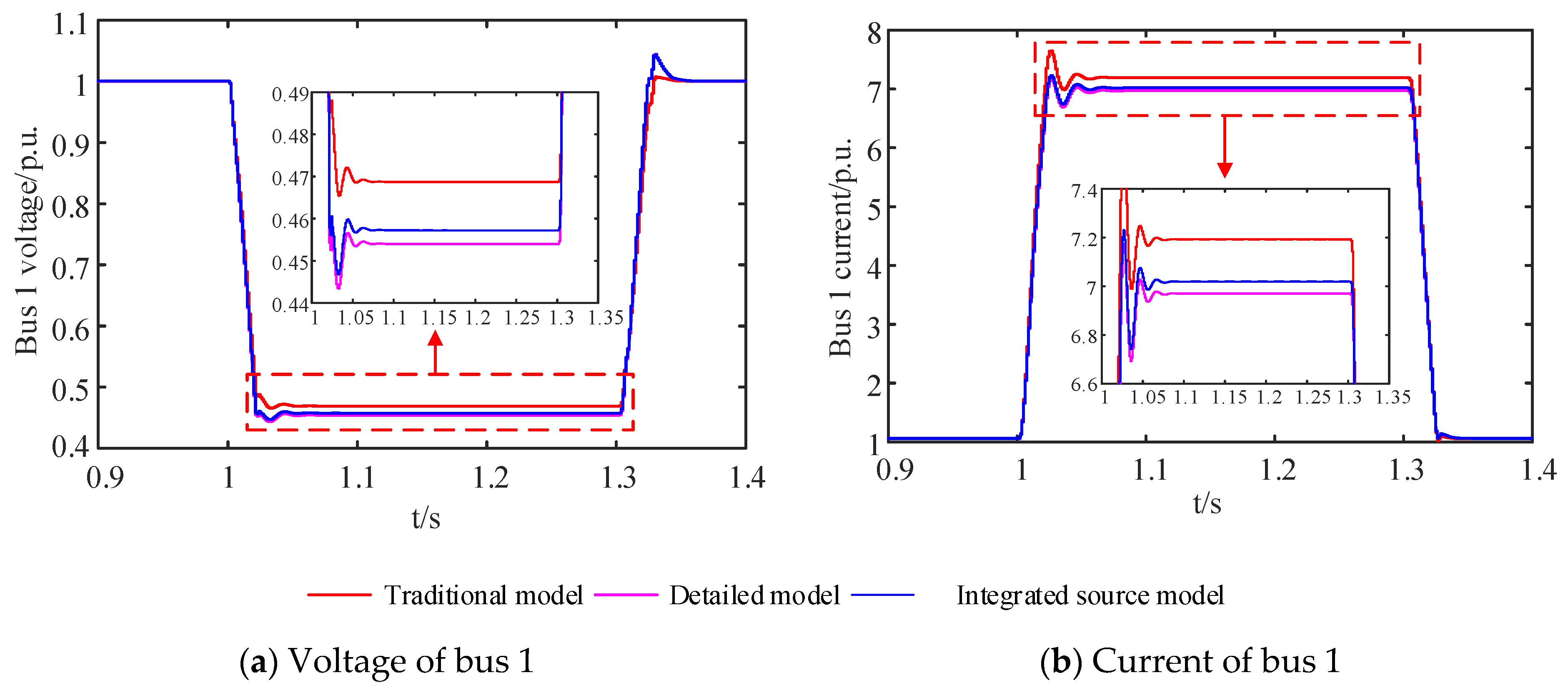
5.1.3. Performance Comparison of Different Models

The existing grid-side source models for distribution network fault calculation are mostly traditional models that only consider the source characteristics of synchronous generators. In the following section, taking the connection of the 15 MW IBR as an example, the errors of the grid-side bus voltages and currents based on the integrated source model are compared with those based on the traditional model (single synchronous generator source). Different types of faults in the distribution network are simulated. The detailed model shown in Figure 2 serves as the benchmark for comparing the errors.

(a)

Three-phase faults

The faults occur at t = 1.0 s and are cleared at t = 1.3 s. The fault resistance is 0.5 Ω. Figure 11 shows the voltages and output currents of the grid-side bus 1 of the distribution network when three different models are used.

It can be seen that, during normal operation, when the above three models are used, the bus voltage and output current are the same. During three-phase faults, when the detailed model is used, the bus voltage is 0.454 p.u., and the output current is 6.970 p.u. When the traditional source model is used, the bus voltage is 0.469 p.u., and the output current is 7.192 p.u. The voltage errors is 3.304%, and the current error is 3.185%. When the integrated source model is used, the bus voltage is 0.457 p.u., and the output current is 7.019 p.u. Compared with the current and voltage when the detailed model is used, the voltage error of the proposed model is 0.661%, and the current error of the proposed model is 0.703%, both of which are smaller than those of the traditional model. The integrated source model can better reflect the influence of the grid-side IBRs.

(b)

Phase-to-phase faults

Phase-A-to-phase-B fault cases are studied in this section. The simulation results of the sequence components at bus 1 are listed in

Table 3. Positive-sequence component of the fault voltage at bus 1 and the fault current at line 1.

	Detailed Model/p.u.	Traditional Model/p.u.	Integrated Source Model/p.u.	Error 1%	Error 2%
Voltage	0.764	0.761	0.766	0.393	0.262
Current	3.630	3.814	3.653	5.069	0.634

and

Table 4. Negative-sequence component of the fault voltage at bus 1 and the fault current at line 1.

	Detailed Model/p.u.	Traditional Model/p.u.	Integrated Source Model/p.u.	Error 1%	Error 2%
Voltage	0.295	0.262	0.293	11.186	0.678
Current	2.842	3.04	2.865	6.967	0.809

, where Error 1 is the error between the detailed model and the traditional model, and Error 2 is the error between the detailed model and the integrated source model.

As can be seen from the table, when phase-to-phase faults occur in the distribution network, there are relatively large errors in the sequence components of the voltages and currents obtained by the traditional model. The error of the positive-sequence components of the fault current reaches 5.096%, the error of the negative-sequence components of the fault voltage reaches 11.186%, and the error of the negative-sequence components of the fault current reaches 6.967%. In comparison, the errors of the positive-sequence components and negative-sequence components of the fault voltage and current obtained by the integrated source model are very small. The integrated source model can better reflect the output characteristics of the grid side with IBRs connected during faults in the distribution network.

5.1.4. Convergence and Sensitivity to Initial Conditions

The authors thank the reviewer for the comments. The most important initial condition is the range of the identified parameters. In this paper, 0 Ω ≤ Z_S ≤ 100 Ω and 0 kA ≤ I_NEW ≤ 0.5 kA, based on experience. Theoretically, the performance of the GA is not easily affected by the initial conditions. The impact of initial conditions on convergence is then verified through simulation by adjusting the range of the parameter values. The simulation results are listed in

Table 5. Verification of the convergence under different initial conditions.

Initial Condition	$\mathit{Z}\in (0,60),$${\mathit{I}}_{\mathbf{N}\mathbf{E}\mathbf{W}}\in (0,0.3)$		$\mathit{Z}\in (0,100),$${\mathit{I}}_{\mathbf{N}\mathbf{E}\mathbf{W}}\in (0,0.5)$		$\mathit{Z}\in (0,200),$${\mathit{I}}_{\mathbf{N}\mathbf{E}\mathbf{W}}\in (0,1)$
Percentage of New Energy/%	Number of Iterations	Iteration Time/s	Number of Iterations	Iteration Time/s	Number of Iterations	Iteration Time/s
20.0	76	0.198	75	0.200	128	0.273
40.0	79	0.198	75	0.200	105	0.235
60.0	83	0.203	80	0.209	88	0.213
80.0	88	0.212	85	0.214	93	0.220

. It can be seen that the range of parameters has a relatively small impact on the convergence speed, and convergence can be achieved relatively quickly under different initial conditions.

The real-time applicability mainly depends on whether the measured main grid parameters can reflect the real-time grid state and the speed of parameter calculation. The former is determined by the sampling interval of U and I used for identifying the main grid parameters; if the operating state of the main grid remains unchanged or changes slowly within the sampling interval, it is considered to accurately reflect the current grid state. The latter refers to the iteration time. The iteration time obtained from the main grid parameter identification process using Matlab is shown in Table 5. It can be seen that the algorithm has a fast calculation speed and good real-time performance.

5.1.5. Performance of Different Parameter Identification Methods

To further compare the performance of different algorithms, the parameter identification accuracy and convergence performance of each algorithm are verified through simulation, as shown in

Table 6. Parameter identification error and convergence performance of the GA.

Percentage of New Energy/%	Parameters	Set Value/p.u.	Identification Value/p.u.	Error/%	Number of Iterations	Iteration Time/s
20.0	z	0.092	0.091	1.087	60	0.18
	Ipw	0.200	0.196	2.000
40.0	z	0.097	0.096	1.031	86	0.201
	Ipw	0.400	0.395	1.250
60.0	z	0.104	0.102	1.818	64	0.178
	Ipw	0.600	0.595	0.833
80.0	z	0.110	0.108	1.818	80	0.190
	Ipw	0.800	0.797	0.375

and

Table 7. Parameter identification error and convergence performance of the SQP and SA.

System Parameters			SQP [26]				SA [27]
Percentage of New Energy/%	Parameters	Set Value/p.u.	Identification Value/p.u.	Error/%	Number of Iterations	Iteration Time/s	Identification Value/p.u	Error/%	Number of Iterations	Iteration Time/s
20.0	z	0.092	0.091	1.087	43	0.040	0.094	2.455	1078	22.212
	Ipw	0.200	0.196	2.000			0.201	0.738
40.0	z	0.097	0.096	1.031	36	0.047	0.093	3.483	2246	33.769
	Ipw	0.400	0.394	1.500			0.473	18.36
60.0	z	0.104	0.102	1.818	40	0.158	0.098	5.754	1593	25.585
	Ipw	0.600	0.595	0.833			0.583	2.800
80.0	z	0.110	0.106	3.636	42	0.071	0.103	6.757	1022	13.808
	Ipw	0.800	0.797	0.375			0.770	3.767

. Compared with the other two algorithms, GA has smaller identification errors, a more stable performance, and faster convergence speed.

5.2. Verification of the Fault Calculation Method

With a 4 MW IBR connected on the grid side, the parameters of the grid side can also be identified accurately by the integrated source model. These parameters are then applied to the grid side in Figure 7 and Figure 8 through the ratio and phase angle transformation of the transformer. Different fault points and fault resistances are simulated to verify the proposed calculation method. When a three-phase short-circuit fault occurs at F1 and F2, respectively, and the transition resistances are 0.5 Ω and 0.7 Ω, the simulation results listed in

Table 8. Three-phase faults at F1.

Rf		IS (kA)	IDG (kA)	If (kA)	UPCC1 (kV)	UPCC2 (kV)
0.5 Ω	Calculated result	0.3870∠−28.9618°	0.1732∠−121.7635°	4.2197∠−62.9923°	25.7404∠−16.7803°	2.1474∠−64.8885°
	Simulation result	0.3863∠−28.9409°	0.1736∠−118.4739°	4.2083∠−62.6828°	25.7605∠−16.5524°	2.1448∠−64.4551°
	Magnitude error	0.18%	0.23%	0.27%	0.78%	0.12%
	Phase angle error	−0.02°	−3.29°	−0.31°	−0.23°	−0.43°
0.7 Ω	Calculated result	0.3600∠−22.7974°	0.1732∠−100.7185°	3.9394∠−55.9138°	32.0985∠−13.8148°	2.7795∠−56.9737°
	Simulation result	0.3594∠−22.8358°	0.1736∠−98.3580°	3.9237∠−55.6943°	32.0614∠−13.6414°	2.7706∠−56.6945°
	Magnitude error	0.17%	0.23%	0.40%	0.12%	0.32%
	Phase angle error	0.04°	−2.36°	−0.22°	−0.17°	−0.28°

and

Table 9. Three-phase faults at F2.

Rf		IS (kA)	IDG (kA)	If (kA)	UPCC1 (kV)	UPCC2 (kV)
0.5 Ω	Calculated result	0.2210∠−19.4515°	0.1732∠−92.4823°	2.5495∠−51.3567°	43.4365∠9.5583°	2.1397∠−35.4237°
	Simulation result	0.2214∠−19.6275°	0.1736∠−89.5513°	2.5383∠−51.1788°	43.3088∠9.6054°	2.1328∠−35.2608°
	Magnitude error	0.18%	0.23%	0.44%	0.29%	0.32%
	Phase angle error	0.18°	−2.93°	−0.1779°	−0.05°	−0.16°
0.7 Ω	Calculated result	0.2110∠−16.2110°	0.1732∠−84.2697°	2.4049∠−47.8867°	45.5659∠9.6577°	2.4914∠−34.9844°
	Simulation result	0.2104∠−16.3237°	0.1736∠−81.5819°	2.4002∠−47.6408°	45.5461∠9.7954°	2.4887∠−34.7417°
	Magnitude error	0.28%	0.23%	0.20%	0.43%	0.11%
	Phase angle error	0.11°	−2.69°	−0.25°	−0.14°	−0.24°

below are obtained.

Under different fault conditions, the maximum magnitude error is 0.78%, and the maximum phase angle error is 3.29°. The method exhibits fast convergence. The rate depends on the error threshold. It is clear that the proposed method can calculate the electrical quantities in the distribution network accurately and quickly, with IBRs on both the grid side and distribution network side considered.

6. Conclusions

In this paper, an integrated source model for the main grid side and a calculation method for electrical quantities are proposed for distribution network faults to address the issue of traditional models failing to accurately reflect the fault characteristics of distribution networks under high penetration of inverter-based resources (IBRs). The influences of the grid-side and the distribution network-side IBRs are taken into account. The specific conclusions are as follows:

(1)

Compared to the single connection of a synchronous generator source, the addition of the grid-side IBRs leads to a decrease in the grid-side port voltage and a reduction in the fault current output to the distribution network during distribution network faults.

(2)

The proposed grid-side integrated source model uses the parallel connection form of ideal voltage sources with series impedance and voltage-controlled current sources, and the genetic algorithm can accurately identify the integrated source model parameters based on the voltage and current at the grid-side ports during normal operation. The model can effectively reflect the impact of the grid-side IBRs on the distribution network during faults.

(3)

Based on the simplified model of the network, the proposed distribution network fault calculation method uses the iterative calculation error of the PCC voltage as a benchmark. Then, accurate calculation of the electrical quantities during distribution network faults can be performed by the relationship between the voltage and output current of IBRs. The amplitude errors are within 1%, and the phase angle errors are within 4°.

References

1. Ma, X.; Zhen, W.; Ren, H.; Zhang, G.; Zhang, K.; Dong, H. A Method for Fault Localization in Distribution Networks with High Proportions of Distributed Generation Based on Graph Convolutional Networks. Energies 2024, 17, 5758. [Google Scholar] [CrossRef]
2. Chen, G.; Liu, Y.; Yang, Q. Impedance Differential Protection for Active Distribution Network. IEEE Trans. Power Deliv. 2020, 35, 25–36. [Google Scholar] [CrossRef]
3. Banerjee, G.; Hachmann, C.; Lipphardt, J.; Wiese, N.; Braun, M. Adaptive Hybrid Overcurrent Protection Scheme with High Shares of Distributed Energy Resources. Energies 2024, 17, 6422. [Google Scholar] [CrossRef]
4. Yin, X.; Zhang, Z.; Xiao, F.; Yang, H.; Yang, Z. Study on Short-Circuit Calculation Model of Distributed Generators and Fault Analysis Method. Power Syst. Prot. Control 2015, 43, 1–9. [Google Scholar]
5. Chang, Z.; Song, G.; Wang, X.; Guo, S.; Zhang, W.; Jin, X. Analysis on Asymmetric Fault Current of Inverter Interfaced Distributed Generator. In Proceedings of the 2016 China International Conference on Electricity Distribution (CICED), Xi’an, China, 10–13 August 2016; pp. 1–6. [Google Scholar]
6. Dong, Z.; Liu, K.; Zhang, B. A General Fault Current Calculation Method for Distribution Network with Distributed Generation. Power Syst. Prot. Control 2019, 47, 161–168. [Google Scholar]
7. Xu, Y.; Wu, T.; Hu, P.; Wang, N. Fault Recovery Method for Distributed Distribution Network Based on Island Partition. J. Electr. Eng. Technol. 2025, 20, 23–35. [Google Scholar] [CrossRef]
8. Gao, Y.; Shi, H.; Wu, S.; Kong, D.; You, H.; Chen, J.; Xu, S.; Chen, J.F. A Practical Approach for Short-Circuit Current Calculation in IIDG-Integrated Distribution Grid. In Proceedings of the 2022 China International Conference on Electricity Distribution (CICED), Changsha, China, 7–8 September 2022; pp. 1477–1483. [Google Scholar]
9. Pan, G.; Zeng, D.; Wang, G.; Zhu, G.; Li, H. Fault Analysis on Distribution Network with Inverter Interfaced Distributed Generations Based on PQ Control Strategy. Proc. CSEE 2014, 34, 555–561. [Google Scholar]
10. Dai, Z.; Li, C.; Jiao, Y. Low-Voltage Ride Through Model of Inverter-Interfaced Distributed Generator and Its Application to Fault Analysis of Distribution Network. Proc. CSU-EPSA 2018, 30, 16–23. [Google Scholar]
11. Shi, S.; Huang, Z.; Zhang, Y. Improvement of Short-circuit Calculation for distribution network with distributed generation. In Proceedings of the 2021 IEEE 4th Advanced Information Management, Communicates, Electronic and Automation Control Conference (IMCEC), Chongqing, China, 18–20 June 2021; pp. 21–24. [Google Scholar]
12. Wang, Q.; Zhou, N.; Ye, L. Fault Analysis for Distribution Networks with Current-Controlled Three-Phase Inverter-Interfaced Distributed Generators. IEEE Trans. Power Deliv. 2015, 30, 1532–1542. [Google Scholar] [CrossRef]
13. Ye, R.; Wang, H.; Zhang, Y. GCN-Based Short-Circuit Current Calculation Method for Active Distribution Networks. IEEE Access 2023, 11, 140092–140102. [Google Scholar] [CrossRef]
14. Shuai, Z.; Shen, C.; Yin, X.; Liu, X.; Shen, Z.J. Fault Analysis of Inverter-Interfaced Distributed Generators with Different Control Schemes. IEEE Trans. Power Deliv. 2018, 33, 1223–1235. [Google Scholar] [CrossRef]
15. Zhu, G.; Sheng, J. Equivalent Modeling of External Network in New Energy Power Grid Taking Voltage Support into Consideration. J. South China Univ. Technol. Nat. Sci. Ed. 2017, 45, 1–7. [Google Scholar]
16. Xie, D.; Xiao, S. Short-Circuit Calculation Equivalent of External Power Grid Including Inverter Interfaced Distributed Generator and Analysis of Influencing Factors. Power Syst. Techol. 2024, 48, 2967–2976. [Google Scholar]
17. Wang, X.; Wu, H.; Wang, X.; Dall, L.; Kwon, J.B. Transient Stability Analysis of Grid-Following VSCs Considering Voltage-Dependent Current Injection During Fault Ride-Through. IEEE Trans. Energy Convers. 2022, 37, 2749–2760. [Google Scholar] [CrossRef]
18. Zhang, C.; Wu, X.; Xie, X. Research on Low Voltage Ride Through of DG Characteristics Based on GB/T33593 standard. Power Syst. Prot. Control 2019, 47, 76–83. [Google Scholar]
19. She, B.; Li, F.; Cui, H.; Shuai, H.; Oboreh-Snapps, O.; Bo, R. Inverter PQ Control with Trajectory Tracking Capability for Microgrids Based on Physics-Informed Reinforcement Learning. IEEE Trans. Smart Grid 2024, 15, 99–112. [Google Scholar] [CrossRef]
20. Cheng, L.; Xu, P.; Zhang, Q.; Wang, Y. Improved PQ Control Mothod for PV System. In Proceedings of the 2019 IEEE Symposium Series on Computational Intelligence (SSCI), Xiamen, China, 6–9 December 2019; pp. 2914–2920. [Google Scholar]
21. Wei, C.; Shi, X.; Zhou, B.; Liu, Y. Fault Model of Inverter Interfaced Distributed Generator Adopting PQ Control Strategy Considering Current Tracking Capability of Converter. In Proceedings of the 2019 IEEE Innovative Smart Grid Technologies—Asia (ISGT Asia), Chengdu, China, 21–24 May 2019; pp. 1419–1424. [Google Scholar]
22. Li, B.; Mu, R.; He, J.; Wang, W.; Yao, C.; Zhang, Y. Transient Fault Current Calculation Method for the PV Grid-Connected System Considering Dynamic Response of PLL. IEEE Trans. Ind. Appl. 2024, 60, 7537–7547. [Google Scholar] [CrossRef]
23. Han, B.; Li, H.; Wang, G.; Zeng, D.; Liang, Y. A Virtual Multi-Terminal Current Differential Protection Scheme for Distribution Networks with Inverter-Interfaced Distributed Generators. IEEE Trans. Smart Grid 2018, 9, 5418–5431. [Google Scholar] [CrossRef]
24. Liu, H.; Xu, K.; Zhang, Z.; Liu, W.; Ao, J. Research on Theoretical Calculation Methods of Photovoltaic Power Short-Circuit Current and Influencing Factors of Its Fault Characteristics. Energies 2019, 12, 316. [Google Scholar] [CrossRef]
25. Wang, L.; Gao, H.; Zou, G. Modeling Methodology and Fault Simulation of Distribution Networks Integrated with Inverter-Based DG. Prot. Control. Mod. Power Syst. 2017, 2, 1–9. [Google Scholar] [CrossRef]
26. Hasan, M.S.; Kamalasadan, S. Optimization of DER Integrated Distribution System by Sequential Quadratic Programming (SQP). In Proceedings of the 2022 IEEE Global Conference on Computing, Power and Communication Technologies (GlobConPT), New Delhi, India, 23–25 September 2022; pp. 1–6. [Google Scholar]
27. Ekinci, S.; Izci, D.; Yilmaz, M. Simulated Annealing Aided Artificial Hummingbird Optimizer for Infinite Impulse Response System Identification. IEEE Access 2023, 11, 88627–88636. [Google Scholar] [CrossRef]
Figure 1. Dual-loop control structure of a grid-connected inverter in a dq coordinate system.
Energies 18 02111 g001
Figure 2. Schematic diagram of the system taking into account the impact of new energy on the grid side and the distribution network side.
Energies 18 02111 g002
Figure 3. Comparison between a traditional grid-side source model and an integrated source model.
Energies 18 02111 g003
Figure 4. Flow chart of parameter identification based on the genetic algorithm.
Energies 18 02111 g004
Figure 5. A distribution network with a high proportion of new energy sources on the grid side.
Energies 18 02111 g005
Figure 6. Equivalent model of distribution grid faults with a high proportion of new energy sources connected to the grid side.
Energies 18 02111 g006
Figure 7. Simplified equivalent circuit during an F1 fault.
Energies 18 02111 g007
Figure 8. Simplified equivalent circuit at fault F2.
Energies 18 02111 g008
Figure 9. Fault calculation process taking into account the influence of IBRs on the grid side and distribution network side.
Energies 18 02111 g009
Figure 10. Voltages and currents at bus 1.
Energies 18 02111 g010
Figure 11. Voltages and currents of bus 1 when three different models are used.
Energies 18 02111 g011