Real Energy Efficiency of Road Vehicles

Abstract

There is an urgent need for a method of evaluating the real energy performance of vehicles that eliminates the effects of external conditions (topography, altitude, and road conditions) and human factors (driving styles), especially in the case of heavy-duty vehicles. Governmental authorities require results on the energy performance of vehicles to develop strategies that result in reductions in greenhouse gas emissions, while fleet managers require results regarding the energy efficiency of existing vehicle technologies to select the technologies that minimize energy consumption and, therefore, operational costs. Aiming to address this need, we propose a method for evaluating the global energy efficiency of road vehicles by monitoring at 1 Hz the operational variables of a vehicle under normal conditions of use for a long time. The variables monitored are engine RPM and vehicle location, speed, payload, and energy consumption. This method was verified using 49 vehicles, representing 23 vehicle technologies. These vehicles varied in size (light duty and heavy duty), application (cars, buses, and freight), energy sources (gasoline, diesel, and electric), and operational conditions (Chile, Ecuador, Colombia, and México). Testing was conducted across various altitudes (0–3600 masl) and topographies (flat and mountainous regions). The results showed that the energy efficiencies for gasoline-fueled light-duty vehicles ranged from 17 to 30%, those for diesel-fueled heavy-duty vehicles ranged from 25 to 42%, and those for electric heavy-duty vehicles (HDVs) ranged from 70 to 80%.

1. Introduction

The dependence on vehicles powered by internal combustion engines for the transport of people and goods, coupled with the continuous growth of vehicle fleets, positions road transport as a key driver of energy consumption [1,2]. Under these circumstances, fuel consumption is proportional to the tailpipe emissions of (i) air pollutants (CO, NOx, VOCs, and PM), which have negative effects on human health, and (ii) greenhouse gases (GHG), such as CO₂, N₂O, and CH₄, which contribute to global warming. Currently, road transport is one of the primary contributors to the global energy demand and GHG emissions (~45%) [3].

Therefore, mitigating vehicles’ environmental impact is essential for achieving global sustainability. Over the past 50 years, there has been an interest in the emission of air pollutants. However, during the past decade, the interest in GHG emissions has been increasing, and it has become a worldwide priority. The worldwide objective has become to reduce GHG emissions through the adoption of electric vehicles and decrease energy consumption via incrementing the energy efficiency of brand-new vehicles.

The evaluation of the energy efficiency of vehicles is not a new topic. In ground transportation, energy efficiency is commonly associated with metrics such as specific fuel consumption (SFC, L/100 km) or fuel economy (km/L) or their equivalent in CO₂ emissions [4,5,6,7,8]. However, these metrics exhibit great variability because, besides vehicle technology, they are highly influenced by vehicle size (gross vehicle weight), external factors (topography, road conditions, and weather conditions), and human factors (driving habits). Therefore, these metrics do not evaluate the energy efficiency of vehicle technology under real conditions of use.

Thus, to promote the adoption of the most energy-efficient vehicles (or limit the commercialization of the less efficient vehicles), there is a need for a metric for evaluating vehicles’ energy efficiency and a method of evaluating that metric that fulfills the following conditions:

• It should be able to evaluate the performance of a whole vehicle rather than single components of a vehicle.
• The method of evaluation should be repeatable and reproducible. Therefore, it should isolate the effect of external and human factors that may influence vehicle fuel consumption.
• It should be able to evaluate a vehicle under real conditions of use.
• Its evaluation should be independent of vehicle technology, size, or energy source.
• It should have a low cost of implementation.
• It should be useful for decision-making among fleet managers, manufacturers, and governmental parties.

Furthermore, there is a need for baseline values of such metrics that could be used for comparative purposes and the design of new public policies.

1.1. Literature Review

Table 1 lists the existing methods of evaluating the energy efficiency of ground vehicles. Next, we briefly describe them along with their advantages and disadvantages and their applicability to achieving the objective of this work.

Testing the vehicle on a chassis dynamometer: The tractive axes of a vehicle are mounted on the rolls of a chassis dynamometer, the torque provided by the engine as measured at the wheels is measured by the dynamometer while the vehicle completes a driving cycle, and fuel consumption is measured using any available method. Most of the time, the vehicle’s efficiency is expressed as SFC (L/100 km) or fuel economy km/L. This method is well accepted because it isolates the effects of external and human factors on fuel consumption, and it is repeatable and reproducible. However, it relies on the assumption that the driving cycle used during the test represents the local driving conditions, which in most cases is not true or at least hard to demonstrate. It has been well documented that these tests may not fully represent the real-world performance of vehicles in use [4]. Furthermore, results vary depending on the driving cycle used. This method is expensive and cannot be used for large vehicles. Following this method, H. Lohse-Busch et al. [5] tested vehicles using three USEPA driving cycles: the Urban Dynamometer Driving Schedule (UDDS), the Highway Fuel Economy Test (HWFET), and the US06, which features very aggressive accelerations and high-speed sections. Vehicle efficiency was determined by the ratio of the positive energy demanded by the wheel [6] to the energy content of the fuel consumed. They obtained an average energy efficiency of 62%, 45%, and 23% for a fuel cell-powered vehicle, a hybrid electric vehicle, and a conventional gasoline-fueled light-duty vehicle (LDV), respectively.

Testing the engine under lab conditions: This has been the preferred method for the case of heavy-duty vehicles (HDVs), which, due to their large size and weight, cannot be tested on a chassis dynamometer. In this case, fuel consumption is measured using the gravimetric method, while the engine output power is measured using an engine dynamometer while the vehicle completes a pre-established load cycle. Efficiency is expressed as the fuel rate consumed per unit of output power (L/kWh). Clearly, this method does not satisfy the requirements of describing the performance of the overall vehicle. B. Wang et al. [7] tested 13 L six-cylinder engines running at 1038 RPM using an engine test bench. They found brake thermal energy efficiencies of 47.1% and 48.7% for diesel and gasoline–ethanol-fueled engines, respectively. The analysis was complemented by an energy and exergetic analysis, which showed that between 26% and 28% of the energy was lost through the combustion process. P. Divekar et al. [8] evaluated a 6.2 L, normally aspirated, spark-ignited eight-cylinder engine. The combustion process was evaluated by measuring cylinder pressure and heat release. Two types of fuel were used: gasoline and natural gas (CNG). The tests were carried out under different load conditions, obtaining a maximum brake thermal efficiency (BTE) of 36.4% for the case of CNG and 35.3% for gasoline. Z. Zhu et al. [9] tested a 10.98 L six-cylinder, spark ignition, pure-methanol engine in an engine dyno in order to compare the overall performance improvement over a CNG engine. Engines were tested at different loads (40%, 60%, 80%, and 100%) in the 800–1800 RPM range. A peak of 41% of BTE was obtained for the pure methanol engine, which can be compared to 38.4% for the CNG engine. Mulholland et al. [10] reported the average BTE of several engine technologies obtained using the World Harmonized Transient Cycle (WHTC). They reported that the most efficient engines in the European market had a maximum efficiency of 43%. The previous work provides maximum reference values for the energy efficiency of vehicles.

On-road tests: In this case, the vehicle’s fuel consumption is measured while the vehicle completes a representative driving cycle on a track. Energy efficiency is expressed as the proportion of fuel energy content that is converted into power to propel the vehicle and its load (freight or passengers). This method is repeatable and reproducible at low cost. However, there is still disagreement about the method used to determine the power needed to propel the vehicle. It also suffers from the issue of the lack of representativeness involved in the use of a driving cycle. Following this methodology, H. Li. [11] instrumented a car with a fuel flow meter, a GPS, and an air/fuel ratio sensor. The vehicle completed a typical driving cycle on the streets of Leeds. The thermal efficiency was determined via the relationship between the power obtained on the output shaft and the energy delivered by the fuel. The power at the shaft was estimated as the product of the vehicle-specific power (VSP) and vehicle mass. VSP was estimated with a simplified equation that is a function only of vehicle speed. They observed an efficiency of 8% during hours of high vehicular traffic and 20% during fluid traffic for a gasoline-fueled LDV, indicating that their method did not yield reproducible results.

Computer simulation: Given the difficulty of evaluating large vehicles in laboratory settings, environmental authorities have developed computational methods to predict such vehicles’ energy performance. The models most well known are the GEM (Greenhouse Emissions Model), developed by the USEPA, and the VECTO (Vehicle Energy Consumption Calculation Tool), which was developed by the European environmental authorities. These models are used for regulatory purposes. Both models provide outputs for specific fuel consumption (L/100 km and L/100 t km, or their equivalents) and CO₂ emissions. While they consider similar factors, they are customized to meet the requirements of their respective markets. Additionally, both models require engine operation maps to determine fuel consumption and CO₂ emissions accurately. The authors of [12,13,14] simulated the operation of a vehicle considering the engine, power transmission, exhaust, and energy recovery system. The tests were simulated according to the New York City Cycle (NYCC) and revealed that the energy recovery system could increase vehicle energy efficiency by up to 5.50%. A. Yadav et al,. [15] estimated the potential reductions in CO₂ emissions and energy consumption generated by various degrees of stringency of standards for heavy-duty trucks in India.

The cited authors used Amesim simulation software (https://plm.sw.siemens.com/en-US/simcenter/systems-simulation/amesim/, accessed on 12 March 2025) to test different truck models and then defined five levels of engine efficiency that could be achieved in an eight-year time frame. For this case, the highest level of braking thermal efficiency (BTE) used was 55%, according to the Super Truck Program target. The authors of [16,17] proposed an improvement of the method for assessing the energy efficiency of vehicles, taking into account the road loads under normal operating conditions. They developed a function that expresses the mechanical energy in traction mode as a function of other operating variables. The proposed function considers various traction modes of a vehicle along a given route as well as road resistance, the aerodynamic parameters of the body, and the mass of the vehicle, including its payload. These factors collectively determine the actual load on the structure during transport. Although the results were not expressed as a percentage of efficiency, they provide valuable insights into a vehicle’s performance.

Table 1. Review of the literature about obtaining the energy efficiency of engines and vehicles.

Method		Authors	Place	Objective	Conditions	Equation	Conclusion
Simulation	Engine	Casisi et al., 2020 [18]	Italy	Increase the energy efficiency of a naval engine with energy recovery	Simulation of operation at maximum load	${\eta }_b={\displaystyle \frac{{\dot{W}}_b}{{\dot{W}}_{in}}}$	Brake efficiency of 49% and an increase of power output of 10% were observed
	Vehicle	Wang et al., 2020 [14]	China	Increase the energy efficiency of a heavy-duty vehicle with energy recovery using the ORC system.	GT suite software (https://www.gtisoft.com/gt-suite/, accessed on 12 March 2025) simulating NYCC and highway driving cycles	${\eta }_{ORC}={\displaystyle \frac{{\dot{W}}_{exp}-{\dot{W}}_p}{{\dot{Q}}_{exh}}}$	Energy recovery efficiencies of ORC of 1.4% and 5.5% were observed for each condition
		Yadav et al., 2023 [15]	India	Evaluate the energy efficiency of HDT under Indian conditions	Simulated using Amesim software using duty cycles based on real-world data	NA	Top BTE of 55% was achieved through several engine improvements
Laboratory	Engine	B. Wang et al., 2019 [7]	China	Test and understand energy and exergy loss mechanisms for ICE	Heavy-duty diesel engine tested in an engine-dyno Engine testing at 1038 RPM	${\eta }_i={\displaystyle \frac{PV}{m_{f}LH{V}_f}}$	A top indicated brake thermal efficiency of 47% was achieved
		Divekar et al., 2023 [8]	Canada	Evaluate performance of spark ignition (SI) engines with CNG and gasoline	Maximum load operation	$BTE={\displaystyle \frac{W_{shaft}}{m_{f}LH{V}_f}}$	Top BTEs of 36.4% and 35.2 were achieved for CNG and gasoline, respectively
		Zhu et al., 2022 [9]	China	Test SI engine fueled with pure methanol and determine whether it is an improvement over natural gas	40, 60, 80, and 100% engine load operating conditions on engine dyno.	$BTE={\displaystyle \frac{{\dot{W}}_b}{{\dot{m}}_{f}LH{V}_f}}$	41% top BTE was achieved for pure-methanol engine
	Vehicle	Lohse-Busch et al., 2020 [5]	United States	Evaluate fuel-cell vehicles’ energy efficiency	Chassis dyno test under different EPA driving schedules	${\eta }_{vehicle}={\displaystyle \frac{E{+}_{cycle}}{m_{f}LH{V}_f}}$	Average vehicle efficiency of 62.2% was achieved for FC vehicles
		Mulholland et al., 2023 [10]	Europe	Report the energy and CO2 emissions emitted by trucks	Dynamometer tests for different manufacturers’ trucks under WHTC driving cycle	NA	Maximum braking thermal efficiency of 43% was achieved for a specific manufacturer
On-road	Vehicle	Li et al., 2016 [11]	United Kingdom	Investigate fuel consumption, brake thermal efficiency, and greenhouse gas emissions generated under real-world driving conditions.	Test of a gasoline passenger car under real operating conditions in an urban area, estimating VSP.	${\eta }_b={\displaystyle \frac{VSP·M}{FC·LHV}}$	Braking thermal efficiency of 16–20% was achieved
		Abbdurazzokov et al., 2021 [17]	Uzbekistan	Improve the method for assessing the energy efficiency of a vehicle, taking into account the load under operating conditions	Normal and real operating conditions and operation data analysis	No efficiency metrics were determined	A linear relationship between engine torque and fuel consumption was found

Table 1. Review of the literature about obtaining the energy efficiency of engines and vehicles.

Method		Authors	Place	Objective	Conditions	Equation	Conclusion
Simulation	Engine	Casisi et al., 2020 [18]	Italy	Increase the energy efficiency of a naval engine with energy recovery	Simulation of operation at maximum load	${\eta }_b={\displaystyle \frac{{\dot{W}}_b}{{\dot{W}}_{in}}}$	Brake efficiency of 49% and an increase of power output of 10% were observed
	Vehicle	Wang et al., 2020 [14]	China	Increase the energy efficiency of a heavy-duty vehicle with energy recovery using the ORC system.	GT suite software (https://www.gtisoft.com/gt-suite/, accessed on 12 March 2025) simulating NYCC and highway driving cycles	${\eta }_{ORC}={\displaystyle \frac{{\dot{W}}_{exp}-{\dot{W}}_p}{{\dot{Q}}_{exh}}}$	Energy recovery efficiencies of ORC of 1.4% and 5.5% were observed for each condition
		Yadav et al., 2023 [15]	India	Evaluate the energy efficiency of HDT under Indian conditions	Simulated using Amesim software using duty cycles based on real-world data	NA	Top BTE of 55% was achieved through several engine improvements
Laboratory	Engine	B. Wang et al., 2019 [7]	China	Test and understand energy and exergy loss mechanisms for ICE	Heavy-duty diesel engine tested in an engine-dyno Engine testing at 1038 RPM	${\eta }_i={\displaystyle \frac{PV}{m_{f}LH{V}_f}}$	A top indicated brake thermal efficiency of 47% was achieved
		Divekar et al., 2023 [8]	Canada	Evaluate performance of spark ignition (SI) engines with CNG and gasoline	Maximum load operation	$BTE={\displaystyle \frac{W_{shaft}}{m_{f}LH{V}_f}}$	Top BTEs of 36.4% and 35.2 were achieved for CNG and gasoline, respectively
		Zhu et al., 2022 [9]	China	Test SI engine fueled with pure methanol and determine whether it is an improvement over natural gas	40, 60, 80, and 100% engine load operating conditions on engine dyno.	$BTE={\displaystyle \frac{{\dot{W}}_b}{{\dot{m}}_{f}LH{V}_f}}$	41% top BTE was achieved for pure-methanol engine
	Vehicle	Lohse-Busch et al., 2020 [5]	United States	Evaluate fuel-cell vehicles’ energy efficiency	Chassis dyno test under different EPA driving schedules	${\eta }_{vehicle}={\displaystyle \frac{E{+}_{cycle}}{m_{f}LH{V}_f}}$	Average vehicle efficiency of 62.2% was achieved for FC vehicles
		Mulholland et al., 2023 [10]	Europe	Report the energy and CO2 emissions emitted by trucks	Dynamometer tests for different manufacturers’ trucks under WHTC driving cycle	NA	Maximum braking thermal efficiency of 43% was achieved for a specific manufacturer
On-road	Vehicle	Li et al., 2016 [11]	United Kingdom	Investigate fuel consumption, brake thermal efficiency, and greenhouse gas emissions generated under real-world driving conditions.	Test of a gasoline passenger car under real operating conditions in an urban area, estimating VSP.	${\eta }_b={\displaystyle \frac{VSP·M}{FC·LHV}}$	Braking thermal efficiency of 16–20% was achieved
		Abbdurazzokov et al., 2021 [17]	Uzbekistan	Improve the method for assessing the energy efficiency of a vehicle, taking into account the load under operating conditions	Normal and real operating conditions and operation data analysis	No efficiency metrics were determined	A linear relationship between engine torque and fuel consumption was found

1.2. This Work

The literature review highlights the lack of consensus on the definition of a metric for evaluating vehicles’ real energy efficiency and a method for evaluating it that satisfies the requirements of repeatability and reproducibility, the isolation of other influencing variables, energy source independence, affordability, and practicality. Aiming to address this need, in this work, we propose adopting the fraction of the energy consumed by the vehicles (E_s) that is converted into mechanical work at the wheels (W_x) needed to propel a vehicle as the metric of vehicle energy efficiency. Equation (1) defines this metric, which may be the most accepted among researchers and practitioners worldwide.

$$\eta ={\displaystyle \frac{W_x}{E_s}}$$

(1)

We also propose to take advantage of the advancements in information technology and evaluate this metric by using data gathered (while monitoring at 1 Hz) on vehicle location, vehicle speed, engine (or electric motor) RPM, and instant energy consumption during a representative period with normal working conditions.

Thus, the aim of this study was to demonstrate the applicability of the proposed metric and method of evaluation to accurately measuring the real energy efficiency of vehicles under normal operating conditions using telematics systems across various vehicle technologies operating under normal conditions of use in different countries. In addition, baseline values for the real energy efficiency of different vehicle technologies were established.

This energy efficiency metric and the proposed methodology for evaluating it eliminate the influence of external variables (topography and road conditions) and human influencing factors on the energy consumption of vehicles. They will be useful for fleet managers who are looking to renew their vehicle fleet with technologies that have the best performance for a given task and identify strategies for reducing their energy consumption. It is also useful for governmental authorities who are looking to design public policies that can guide our society in terms of actions that contribute to reducing energy consumption and emissions of air pollutants and GHGs.

2. Methodology

Aiming to demonstrate the applicability of the proposed metric and the method of evaluating it, we followed the methodology illustrated in Figure 1. First, we verified that the proposed methodology for evaluating energy efficiency via telemetry systems produced the same results obtained when a vehicle was tested under laboratory conditions on a chassis dynamometer (Figure 1a). Complementarily, we verified that the proposed methodology produced the same results for a single technology working under very different conditions (normal working conditions with respect to three countries) (Figure 1b). Finally, the proposed methodology was used to obtain the energy efficiencies of common technologies operating under normal conditions of use in several Latin American countries (Figure 1c). Below, we describe each step in detail.

2.1. Regions of Study

Several vehicles were monitored while they were operated under normal conditions of use in several regions.

Table 2. Main characteristics of the regions studied.

Country	Colombia (Col)				Ecuador (Ec)		México (Mx)		Chile
Region	Bogotá	Medellín	Apartadó	Bogotá–Cali logistic corridor	Cuenca—Azogues	Catamayo–Guayaquil highway	Monterrey	Saltillo	Santiago, and mining areas
Location (in the country)	Center	North-west	North-west	West-center highway	Center-south	South-west national highway	North-east		Center, center-west, north
Latitude and longitude (degrees)	4.60971, −74.08175	6.405534, −75.42661	7.873731, −76.65214	Between (3.44, −76.52) and (4.61, −74.081)	−2.9055, −79.00453	Between (−3.99, −79.36) and (−2.19, −79.88)	25.6813, −100.316	25.033, −100.166	−20.82701, −68.64101, −33.45456, −70.78152
Average altitude (masl)	2500	1500	30	1800	2500	600	500	1500	1190
Average positive road grade (%)	1.91	5.01	3.01	6.04	5.01	5.85	3.30	3.67	3.86
Weather	Temperate	Warm and overcast	Hot, humid	Temperate—Hot, humid	Temperate	Tropical—Hot, humid	Hot, semiarid.		Variable conditions
Average annual temperature (°C)	13.1	17	27	13.1 and 20	15	20–25	25	25	12–20
Topography of test zone	Steady, mostly flat roads were selected for the tests.	Steady, mostly flat roads were selected for the tests.	Steady, mostly flat roads were selected for the tests.	Variable (may include regions with high road grade of ascent or descent)
Type of test/driving	On-road under specific driving cycles	Lab test was performed on chassis dyno and on-road under specific driving cycles	On-road under specific driving cycles	Normal driving conditions

describes the main characteristics of these regions.

In Colombia, the vehicles were operated under controlled conditions at different altitudes, including in Bogotá, Medellin, and Apartadó, which are flat regions located at different altitudes (2500; 1200; and 50 masl, respectively).

In Ecuador, they were operated under normal conditions of use on the highway that connects Cuenca and Azogues, a road of varying topography and altitude (~2500 masl). Additionally, in Ecuador, the HDV was driven on round trips between Guayaquil and Catamayo, which involved significant elevation changes from 1200 to 0 masl, passing through diverse landscapes, including coastal plains and mountainous regions.

In the case of México, vehicles were monitored under normal conditions of use in Monterrey and Saltillo. Both cities are located in flat regions in Northeast Mexico at about 600 masl and 1500 masl, respectively.

In Chile, vehicles were driven on various roads with differing topographies and altitudes ranging from 0 to 3500 masl. Here, the terrain includes flat coastal areas, steep mountainous regions, and high-altitude plateaus, each presenting challenges for vehicle performance. Electric buses primarily serve the metropolitan area of Santiago and its surrounding mining regions, where the altitude varies significantly. Similarly, diesel buses were driven near Santiago, heading towards the Pacific coast, as well as in the Bellavista Salt Flat and Salar de Pintados areas. Diesel-fueled buses were also used in the northern region, between Iquique and the Salar de Coposa. In all cases, the topography is highly variable, influencing vehicle performance due to the combination of altitude, steep inclines, and diverse road conditions. Furthermore, variations in the climatic conditions were notable, with temperatures ranging from 0 to 30 °C.

2.2. Vehicles

Table 3. Characteristics of monitored vehicles.

Country	Vehicle ID	Manufacturer and Model	Model Year	Fuel	Category	Local Classification	Reference Classification	Use	GVWR (t)	Test	Test Weight (t)	Payload (t or Pass)	Tests or Trips (#)	No. of Vehicles (#)	Collected Data (#)	Distance (km)	Energy Used (L or kWh)
Col	UEN-882	Renault Logan	2016	Gas	PC	M1—PC	Class 1: LDV	Pass	1.5	DC Dyno, DC on road	1.1	1	3	1	5.4 k	28.9	2.4
	KMZ-274	Foton FKR	2022	Die	B	M3—bus	Class 3: MDV	Freight	5.50	DC on road	5.50	1.76	18	1	33 k	158	13.8
	SNM-050	Chevy NKR	2006	Die	B	M3—bus	Class 3: MDV	Freight	5.50		5.02	1.76	16	2	28 k	113	24
	SNL-915	Chevy NKR	2021	Die	S2T	N2—truck	Class 3: MDV	Freight	5.50		5.02	1.71	17	3	39 k	164	31
	SNM-050 *	Chevy NKR	2006	Die	S2T	N2—truck	Class 3: MDV	Freight	5.50		5.02	1.76
	TRF-533	Chevy NKR	2009	Die	S2T	N2—truck	Class 3: MDV	Freight	5.50		5.02	1.76
	TKE-195	International	1995	Die	B2T	N3—truck	Class 7: MDV	Freight	14.64		14.64	7.00	8	2	20 k	80	39
	VAK-260	Chevy FVR	2020	Die	B2T	N3—truck	Class 7: MDV	Freight	14.64		14.64	7.00
	KMZ-366	Mack Anthem	2020	Die	TT	N3—TT	Class 8: HDV	Freight	52.00		25.18	10.00	39	4	90k	388	244
	KMZ-368	Mack Anthem	2020	Die	TT	N3—TT	Class 8: HDV	Freight	52.00		25.18	10.00
	TRI-494	Mack Anthem	2012	Die	TT	N3—TT	Class 8: HDV	Freight	52.00		24.95	10.00
	TRK-025	Int. Prostar	2013	Die	TT	N3—TT	Class 8: HDV	Freight	52.00		24.95	10.00
	WOL-265	Int. Prostar	2020	Die	TT	N3—TT	Class 8: HDV	Freight	52.00	NO	45.00	34.00	3	1	160k	1200	750
Mx	VWTig	Volkswagen Tiguan	2014	Gas	PC	LDV—PC	Class 1: LDV	Pass	2.34	NO	2.08	3	100	5	200k	2314	177
	KiaR	Kia Rio HB	2017	Gas	PC	LDV—PC	Class 1: LDV	Pass	1.64		1.12	2
	VWJetta	Volkswagen Jetta	2019	Gas	PC	LDV—PC	Class 1: LDV	Pass	1.97		1.40	2
	Seat Ateca	Seat Ateca	2019	Gas	PC	LDV—PC	Class 1: LDV	Pass	1.93		1.35	2
	Yaris	Toyota Yaris	2023	Gas	PC	LDV—PC	Class 1: LDV	Pass	1.60		1.10	2
	L200	Mitsubishi L200	2010	Die	LT	LDV—LT	Class 1: LDV	Mixed	2.85		2.00	5p and 0.7t	2	1	59k	1300	118
	T09	Int. Prostar	2021	Die	TT	N3—TT	Class 8: HDV	Freight	52.00		25.00	14.00	13	2	79k	1232	423
	92	Int. Prostar	2019	Die	TT	N3—TT	Class 8: HDV	Freight	52.00		30.00	19.00
Ec	Kwid	Renault Kwid	2023	Gas	PC	M1—PC	Class 1: LDV	Pass	1.3	NO	0.80	2	31	1	61.2k	572	34
	ZAA2468	Int. Prostar	2021	Die	TT	N3—TT	Class 8: HDV	Freight	52.00		50 and 23 **	41 and 13.6 **	5	1	182k	1992	960
Chile	Electric buses (BE 1—10)	King Long (x10)	2020	Elec	E-B	Pullman—B	Class 8: HDV	Pass	19.00	NO	14.00	41	1646	10	4.29M	108,083	147,022
	MB buses (B—8XX)	Mercedes Benz (x10)	2020	Die	B	Pullman—B	Class 8: HDV	Pass	19.00		18.00	41	525	16	15M	239,772	94,089
	Sc buses (B—7XX)	Scania (x6)	2020	Die	B	Pullman—B	Class 8: HDV	Pass	19.00		18.00	41

Gas: gasoline; Die: diesel; Elec: electricity; B: bus; LDVs: light-duty vehicles; MDVs: medium-duty vehicles; HDVs: heavy-duty vehicles; PC: passenger car; S2T: small two-axle truck; B2T: big two-axle truck; TT: tractor-trailer; GVWR: gross vehicle weight rating. * SNM-050 chassis body is commonly used as a truck or bus; therefore, it was tested with truck and buses driving cycle. ** Round trips on the same route (unloaded—one-way, and full load—return trip).

describes the vehicles monitored in this study. These vehicles fall under a variety of sizes and categories, such as passenger cars, buses, trucks, and HD trucks. This table specifies their classifications according to the gross vehicle weight rate (GVWR) following the US standard [19] and the local classifications. In Colombia and Ecuador, vehicle classification is made by referring to the consolidated resolution “UNECE/TRANS/WP.29/78/Rev.6” adopted by the World Forum for the Harmonization of Vehicle Regulations of the United Nations [20,21]. México has adopted the system used by the United States Federal Highway Administration (FHWA) [22]. In Chile, interurban buses are classified as “Pullman” according to TRANSPORTES, 2017 [23].

2.3. Instrumentation

Table 4. Technical specifications of the instrumentation used in this work.

Device	Country	Monitored Vehicles	Model	Frequency (Hz)	Acquired Signals (Units and Precision)	Other Specifications
OBD interface	Mx, Ec	PC monitored in both countries	OBD-Link Lx	1	Fuel flow rate (L/s, ±0.01) Position: lat and long (degrees, ±1 × 10−5) Vehicle speed (km/h, ±1) Engine speed (RPM, ±5)
GO9/Geotab	Col, Mx, Ec	International Prostar trucks	GO9 device	1/15	Accumulated fuel (L, ±0.1) Position: lat and long (degrees, ±1 × 10−5) Vehicle speed (km/h, ±1) Engine speed (RPM, ±5)
AF ratio analyzer	Col	Vehicles following DC (on road, dyno)	$\mathrm{Horiba}\mathrm{MEXA}\text{-}730\lambda$	1	Air fuel ratio (-, ±0.01) Lambda factor (-, ±0.01)	AFR range: 3.99–500 Lambda range: 0.275–300
MAF			Nippon Denso Toyota MAF Sensor	1	Air mass flow (g/s, ±0.01)
Chassis dynamometer		PC: Logan	Mustang Power Dyne PC	2	Roller torque (Nm, ±0.1) Roller angular speed (RPM, ±5)
Inway-CAN	Chile	Electric and diesel buses	Inway-Can	1/7	Accumulated energy (L or kWh, ±0.1) Position: lat and long (degrees, ±1 × 10−5) Vehicle speed (km/h, ±1) Engine speed (RPM, ±5)

reports the technical specifications of the instrumentation used in this work. In México and Ecuador, vehicles were instrumented with an On-Board Diagnosis (OBD) interface (brand: OBD-Link Lx), which, via the vehicle’s OBD port, reads information derived from the Engine Control Unit (ECU) about the different sensors connected to the engine. A telematics service provider (Geotab, GO9 device) monitored the normal operation of the vehicles using this device. Similarly, in Chile, vehicles were monitored by INWAY, another telematics service provider that uses its own device called ’Inway-can.’ This device retrieves information from the CAN-Bus (Controller Area Network) of both diesel and electric vehicles.

Readings of vehicle location, vehicle speed, engine (or motor) speed, and fuel (or electric energy) consumption were collected with a 1 Hz frequency. The GPS used in this work provided location with an error of less than 3 m. Pepper, and Quirama et al., [24,25] compared the fuel consumption values obtained via OBD with that obtained using the standard gravimetric method specified by [26] and confirmed that they were equivalent, with relative errors smaller than 3%.

In Colombia, fuel consumption was determined through the use of a mass-air-flow (MAF) sensor and a Horiba MEXA-730$\lambda$ air/fuel ratio analyzer. Both measurement systems collect data at 10 Hz. These measurements were synchronized according to the methodology suggested by Giraldo et al. [27]. The chassis dynamometer used was a Mustang Dynamometer Power Dyne PC, which deploys eddy-current power absorbers for precise load control and real-time data on speed, torque, and power. With a roller diameter of 8.75 inches, it allows for accurate simulation of real-world driving conditions [28].

2.4. Monitoring Campaign

Vehicles were monitored while following a local driving cycle using a chassis dynamometer while engaging in the same driving cycle on a track of paved, flat roads at different locations or for a long time under normal conditions of use. Table 3 identifies the conditions of observation for each vehicle. Approximately 965 k data points were collected second by second, with a total of 9600 km traveled and 2.9 k L of fuel (gasoline and diesel) consumed.

In México, Ecuador, and Chile, the vehicles were monitored under normal operating conditions. In México, the five gasoline-fueled LDVs and the diesel-fueled LDT were driven in in Monterrey, while the two diesel-fueled HDVs were driven in Saltillo. In total, the eight vehicles traveled 4800 km and completed 115 trips.

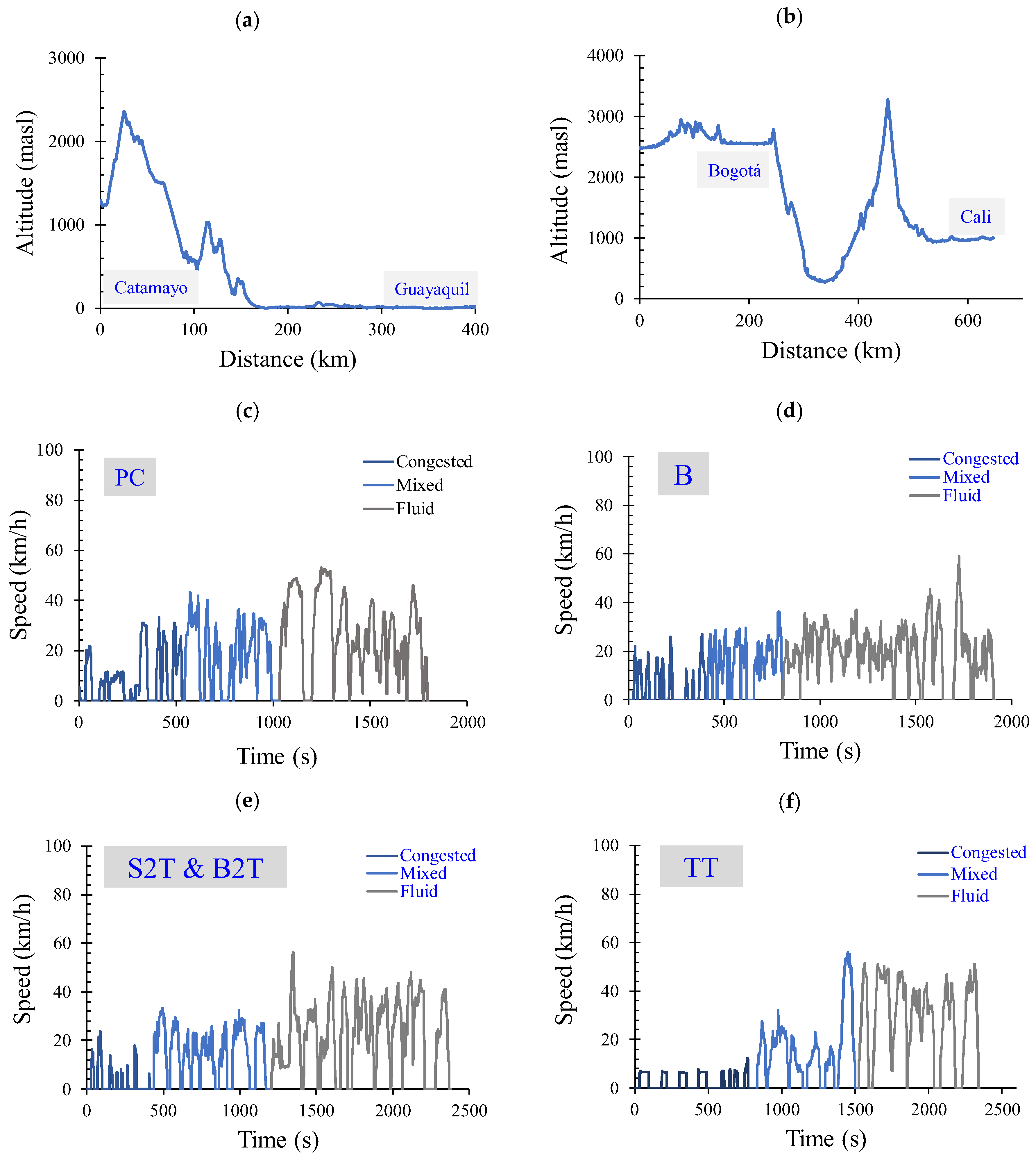
In Ecuador, the gasoline-fueled Renault Kwid was driven mostly between Cuenca and Azogues, which are non-flat urban regions, while the International Prostar+ diesel-fueled HDV completed round trips between Guayaquil and Catamayo. These vehicles traveled 2500 km and completed 36 trips during the monitoring campaign. Figure 2a shows the altitude profile for the Guayaquil and Catamayo roads.

In Bogotá, Medellín, and Apartadó, Colombia, vehicles were tested under local representative driving cycles based on their category. These driving cycles were determined using the Microtrips (MT) method [29]. The driving cycles included three traffic conditions, namely, congested, fluid, and mixed, with their speed–time profiles shown in Figure 2c–f. The tests in Bogotá were conducted in the El Rosal area, located 40 km from the city’s historic center. In Medellín, testing took place on a chassis dynamometer at Institución Universitaria Pascual Bravo under controlled laboratory conditions, as well as on the Hatillo-Girardota highway, located 27 km from the city center. In Apartadó, the vehicles were tested on the lateral highway 8 km from the city center. A total of 101 trips were completed, covering a distance of 931 km. Additionally, a 2020 International Prostar+ heavy-duty truck was monitored during its normal operation between Cali and Bogotá, traveling 1200 km over three trips. Figure 2b shows the altitude profile for the Bogotá–Cali road. Additionally, a Renault Logan was tested while completing a driving cycle, as specified in Table 3, both using a chassis dynamometer located in Medellín and on the road in Bogotá, Medellín, and Apartadó. Data from the Colombian vehicles were obtained from UPME [30], who developed these tests within the framework of the FECOC+ Project, which aimed to obtain the emission factors for Colombian fuels.

In Chile, 10 electric buses and 16 diesel-fueled buses were monitored during their normal operations over a period of five months (October 2022–February 2023). The electric buses covered 108,000 km and 1646 trips, while the diesel buses traveled 239,000 km and completed 525 trips. These vehicles were employed for passenger transport between the major cities (Santiago and Iquique) and nearby mining areas. The altitude variation observed along these routes is comparable to that of Ecuador and Colombia, as all three countries are crossed by the Andes Mountain Range.

2.5. Data Quality Analysis

We considered data only when the vehicle’s engine was running, meaning the engine speed was above the idle range (>500 RPM). Data were disregarded when the vehicle speeds were outside physically plausible values (0–120 km/h). For tests conducted reproducing driving cycles, test results were accepted when the profiles obtained from the monitored vehicle had a relative difference of less than 5% from the speed–time profile of the original driving cycle data. For vehicle energy efficiency evaluation, trips or tests with SFC values above the 99th percentile or below the 1st percentile for each vehicle category were discarded. In previous and subsequent sections, only valid data are reported following the aforementioned data quality analysis.

2.6. Specific Fuel Consumption Comparison

To compare energy consumption between technologies that use different energy sources, we expressed fuel consumption in terms of diesel equivalent liters (DEL). In Chile, the energy content of one liter of diesel is 38.3 MJ [31]. In this context, 1 DEL of electric energy corresponds to the average electric energy that the national electricity generation system can produce with 38.3 MJ (10.64 kWh) of energy.

Table 5. Electricity generation of the National Energy Generation System in Chile.

Source	Generation	Efficiency
	%	%
Petroleum	10%	30
Natural gas	15%	46
Coal	13%	39
Biomass	2%	11
Geothermal	0.3%	90
Eolic	13%	90
Solar	24%	90
Hydraulics	22%	90
Efficiency (${\eta }_g$)		69

presents the fuel mixes used for electricity generation in Chile, along with their corresponding thermal efficiencies. To determine the equivalent energy consumption, we assumed there was 90% efficiency for renewable energy sources, resulting in a weighted average efficiency of 69%. Thus, it was concluded that 7.33 kWh of electric energy is equivalent to 1 DEL. Following this reasoning, the USEPA established that 7.41 kWh of electricity is comparable to 1 US liter of diesel in terms of energy content [31,32].

Additionally, the fuel consumption of gasoline vehicles was also expressed in terms of DEL.

Table 6. Properties of liquid fuels used for road transportation in Colombia, México, and Ecuador.

Country	Colombia		México		Ecuador
Fuel	Diesel	Gasoline	Diesel	Gasoline	Diesel	Gasoline
Lower heating value (MJ/kg)	42.42	40.66	45.66	47.77	42	43
Fuel density (g/L)	851.9	741.2	826	739	820	730
1 DEL (L)	1	1.20	1	1.07	1	1.10
Source	UPME, 2016 [33]		INECC, 2014 [34]		INEN, 2011 and 2012 [35,36]

shows the typical properties of diesel and gasoline in Colombia, México, and Ecuador and the equivalent units in DEL.

2.7. Data Analysis

Equation (1) defines the metric that could be considered the most accepted for evaluating vehicle energy efficiency. It is defined as the ratio of the energy delivered by the source (E_s) to the energy converted into the mechanical work performed via the tractive force at the wheel–road interphase (W_x). It is equal to the work needed to propel the vehicle while traveling under certain external conditions, i.e., road grade, rolling resistance, and aerodynamics conditions, and satisfying the driver’s speed and acceleration requirements [37].

$$E_s={\rho V}_{f}LHV$$

(2)

$$E_s=\int VIdt$$

(3)

The energy source could be the chemical energy content of the fuel consumed for the case of vehicles powered by internal combustion engines (Equation (2)) or the electric energy delivered by the battery pack (Equation (3)) for the case of electric vehicles. In Equations (2) and (3), ρ is density, $V_f$ is the accumulated volume of fuel consumed, LHV is the lower heating value of the fuel, V is the nominal voltage, and I is the current supplied by the battery.

It is important to highlight that the evaluation of this metric should exclude periods of idling and should be performed during a representative period of operative time or over a whole driving cycle.

For tests conducted on a chassis dynamometer while a vehicle is engaging in a driving cycle, the total work done by the tractive force is measured by the time integral of the power sensed by the chassis dynamometer at the vehicle wheel, which is equal to the measured torque ($\tau$) multiplied by roller angular speed (${\omega }_d$).

$$W_x=\int P_{x}dt=\int {\tau \omega }_{d}dt$$

(4)

For tests conducted on roads under a driving cycle or with the vehicle operating under normal conditions of use, the total work done by the tractive force is also calculated by the time integral of the power delivered at the wheel ($P_x$). However, in this case, $P_x$ is estimated as the product of the tractive force ($F_x$) and the vehicle speed (V) (Equation (5)). $F_x$ is the force needed to counteract the rolling resistance ($R_x$), drag ($F_d$), gravity ($F_g$), and inertial ($M{m}_{f}a$) forces, which are calculated through Equations (6)–(11) [38].

$$W_x=\int P_{x}dt=\int F_{x}Vdt$$

(5)

$$F_x=F_i+R_x+F_d+F_g$$

(6)

$$F_i=M{m}_{f_i}a$$

(7)

$$R_x=f_{r}Mg\cos \theta$$

(8)

$$F_d={\displaystyle \frac{1}{2}}{c}_d{A}_f{\rho }_{air}{V}^2$$

(9)

$$F_g=Mg\sin \theta$$

(10)

$$m_{f_i}=1+0.04\left(N_{T{D}_i}\right)+0.0025{\left(N_{T{D}_i}\right)}^2$$

(11)

The variables in this equation are defined below:

M: total vehicle weight;

V: vehicle speed;

a: vehicle acceleration;

fr: rolling resistance coefficient;

$\theta$: road grade;

$c_d$: drag coefficient;

$A_f$: drag area;

${\rho }_{air}$: air density;

$N_{T{D}_i}$: in-use transmission ratio;

$m_{f_i}$: mass factor for equivalent mass;

$F_g$: gravitational force;

$F_d$: drag force;

$R_x$: rolling-resistance force;

$F_i$: inertial force (translational and rotational);

$F_x$: tractive force;

$P_x$:traction power;

$W_x$:traction work.

Thus, according to Equation (1), a vehicle’s global efficiency is the slope of the W_x vs. E_s plot, which can be obtained after performing a linear regression analysis between these two variables.

3. Results

Next, we will present the results obtained by following the methodology described in the previous Section. Initially, we will present the results of the test designed to demonstrate the applicability of the method proposed to measure a vehicle’s energy efficiency. Then, we will present the results establishing the baseline of the energy efficiency of vehicles in LATAM.

3.1. Validation of the Method of Determining Energy Efficiency

The same vehicle engaging in the same driving cycle on a chassis dynamometer and on the road: As previously mentioned, an in-use gasoline-fueled vehicle (Renault Logan) was tested, reproducing the same driving cycle (Figure 1a) on a chassis dynamometer and on the road, in cities located at three different altitudes.

Figure 3a shows that the fuel consumption of this vehicle was (9.00 ± 0.05 L/100 km) when tested on a chassis dynamometer in Medellin. Our analysis of variance (F = 3.79, p = 0.093) indicates that this vehicle exhibited a similar level of fuel consumption when tested on the road in the same city. This means that the tests were conducted correctly and that the testing method for determining SFC yields repeatable and reproducible results, as expected because it is a well-accepted testing protocol (SAE J1082). Similarly, Figure 3b shows that this vehicle exhibited an energy efficiency of (13.59 ± 0.10%) and that this result is statistically similar to the one obtained when the vehicle was tested on the road in the same city (14.95 ± 1.03%). Thus, this result confirms that the method for determining energy efficiency via on-road tests, following the methodology proposed above, yields repeatable and reproducible results. Figure 3a,b also show that altitude has a negligible effect on the fuel consumption and energy efficiency of this vehicle.

The same technology used in different regions: The second alternative for validating the applicability of the method of determining the energy efficiency of vehicles by monitoring their normal operating conditions was to observe a single vehicle operating under very diverse conditions of operation. We expected the vehicles to exhibit the same performance based on the assumption that all the vehicles employed the same technology, were recent models, and were well maintained.

As shown in Table 3, five International Prostar vehicles were monitored in this study. One was driven according to the driving cycle shown in Figure 2 in Bogota, Colombia, and four were driven under normal operating conditions across three different countries: one vehicle in Colombia, two vehicles in México, and one in Ecuador.

Table 7. Operational parameters under which a sample of vehicles produced by the same manufacturer (International Prostar) were driven in three countries. DC: driving cycle displayed in Figure 2f. NO: normal operating conditions described in Section 2.4.

Country	Colombia		México	Ecuador
Type of test	DC	NO	NO	NO
Time (s)	20k	162k	79k	183k
Distance (km)	83.75	1202	1232	1992
Fuel (L)	53.58	851	429	960.34
Activity (t-km)	837.4	40,861	17,157	58,886
SFC (L/100 km)	63.97	70.84	35.03	48.19
SFC* (L/100 t km)	6.39	2.08	2.62	1.63
Average speed (km/h)	15.03	27.50	55.94	39.32
Average positive acc (m/s2)	0.39	0.21	0.29	0.26
Average negative acc (m/s2)	−0.41	−0.26	−0.41	−0.33
Uphill percentage (%)	16%	30%	9%	24%
Downhill percentage (%)	14%	35%	8%	22%
Flat road percentage (%)	70%	35%	83%	54%
Average positive road grade (%)	4.22%	5.81%	3.18%	4.62%
Average negative road grade (%)	−4.09%	−5.98%	−4.57%	−4.51%
Idling percentage (%)	37%	8%	16%	9%
Acc percentage (%)	21%	9%	15%	17%
Deccel. percentage (%)	21%	8%	11%	13%
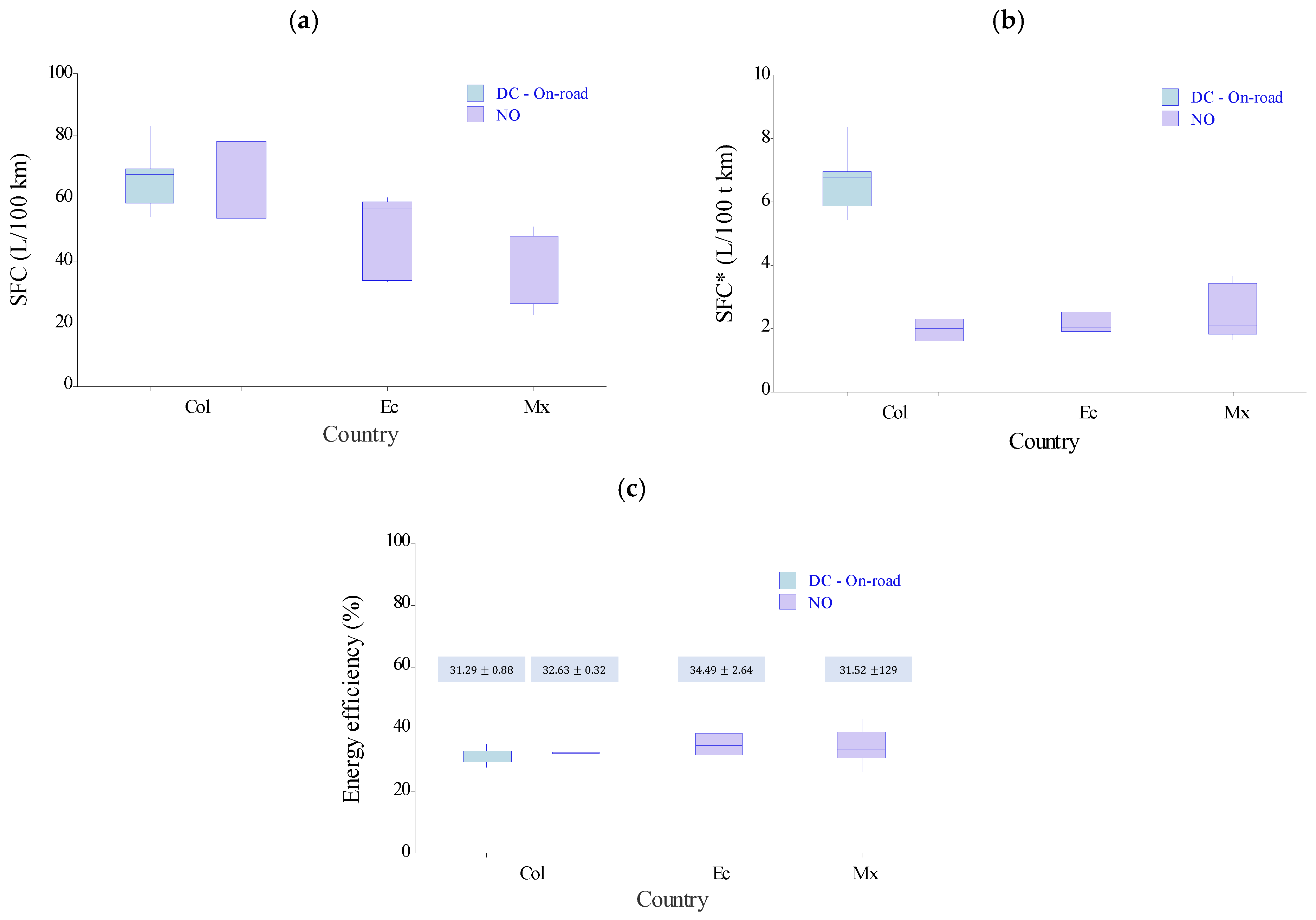
Cruising percentage (%)	21%	74%	58%	61%

lists the key operational parameters pertaining to the vehicles in each country, while Figure 4a,b present their SFC and SFC*, respectively. Table 7 shows that these vehicles were used under diverse operational conditions. For example, the average speeds were 27.50, 55.94, and 39.32 km/h when the vehicles were driven in Colombia, México, and Ecuador, respectively. As expected, their SFC varied according to the influence of external factors (70.84, 35.03, and 48.19 L/100 km in Col, Mex, and Ecu, respectively). Similarly, the SFC* results were different (Table 7). These results confirm that SFC and SFC* are not appropriate indicators for describing the energy efficiency of vehicles because they are influenced by factors other than vehicle technology.

Additionally, Figure 4c displays the energy efficiency observed for these vehicles. After conducting an ANOVA for differences in the mean values obtained for energy efficiency, we concluded that they were statistically equivalent. The ANOVA conducted to compare the means across these technologies did not reveal statistically significant differences between the groups (F = 0.69, p = 0.234). The 95% confidence intervals for the means of each group overlap, and the pooled standard deviation was 5.33, indicating similar variability among the vehicles. These results indicate the following:

• The energy efficiency of vehicles can be determined using the model described in Section 2.7, which uses a vehicle’s daily operative variables (location, engine RPM, speed, fuel/energy consumption, and payload), which can be monitored by telemetry systems.
• The technique yield repeatable and reproducible results. It is independent of conditions of use, external factors (topography and weather), or human factors (driving style).
• The determination of the energy efficiency of vehicles by observing their daily operation leads to the same results that would be yielded when a vehicle is evaluated on a chassis dynamometer regardless of the driving cycle used.

3.2. Vehicles’ Baseline Energy Efficiency

Next, we will describe the results regarding fuel consumption and energy efficiency found by applying the methodology described in Section 2.6 and Section 2.7 to the 23 vehicles described in Table 3.

3.2.1. Specific Fuel Consumption

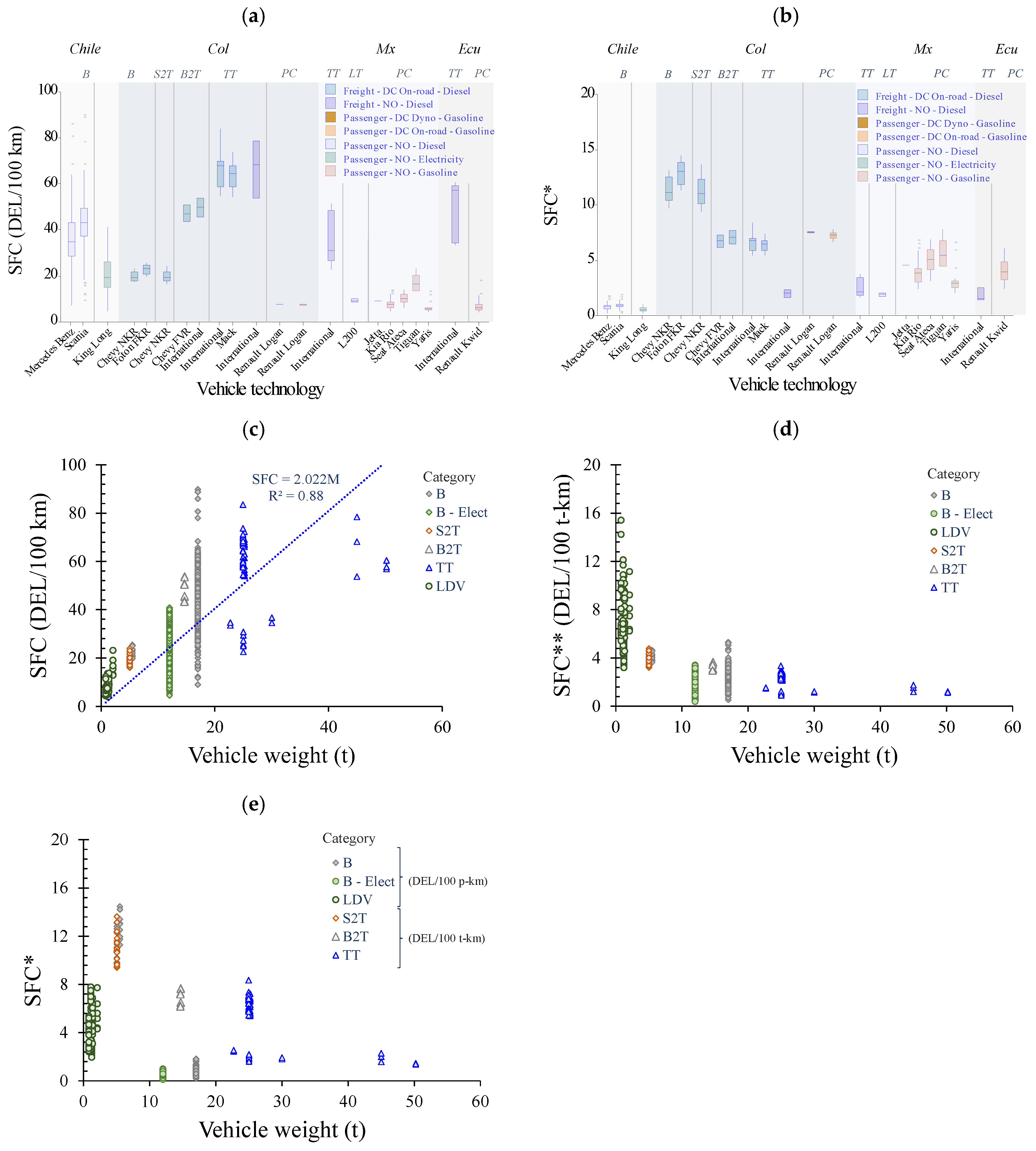
Figure 5 shows the results regarding SFC (5.a) and SFC* (5.b) for the technologies monitored in this study as a function of vehicle category. Traditionally, the specialized community has been interested in these results because they provide insights into the energy efficiency of vehicles useful for decision-making processes engaged in by fleet managers and governmental authorities.

However, these results cannot be used as a baseline for the comparison of the performances of the vehicles. Figure 5 shows that SFC and SFC* exhibit large differences among vehicle categories and among countries. Furthermore, SFC exhibits great variability within the same category (denoted by the sizes of the boxes). These results were expected, as SFC depends directly on the conditions of the vehicles’ use. For example, tractor-trailers (TT) in Colombia have about double the SFC that TTs have in México, which is mainly due to large differences in these countries’ topographies.

Figure 5c shows that SFC is highly correlated with GVWR (R² = 0.88). Thus, by dividing the SFC by its GVWR, the resulting metric (SFC**) should exhibit a constant value among the different categories. Figure 5d shows that the variations are small for GVWR > 10 t. However, this figure evidences that there are other relevant influencing factors, especially for light-duty vehicles (GVWR < 2 t).

Some specialists prefer to divide SFC by the transported payload or the number of passengers moved to obtain SFC* (L/100 t-km and L/100 p-km, respectively) as a metric of vehicle efficiency. This metric has the merit of being oriented toward quantifying the energy consumed for the specific purpose for which a vehicle is being used, that is, liters of fuel used per kilometer traveled and tons of freight transported or passengers transported. However, besides vehicle technology, this metric is influenced by the conditions of use (Figure 5e). Thus, this metric is useful for situations where the conditions of use of vehicles are similar, but it cannot be used to compare vehicle technologies.

3.2.2. Baseline Energy Efficiency

Figure 6 and

Table 8. Energy efficiency and specific fuel consumption results.

Country	Vehicle Category	Test and Fuel	Energy Source	$\mathit{\eta }$ (%)	SFC (DEL/100 km)	SFC* (DEL/100 t km) or (DEL/100 p km)	Manufacturer * SFC (DEL/100 km)
Chile	B	NO	Diesel	$29.04\pm 0.48$	$39.24\pm 0.96$	$0.80\pm 0.02$	NA
		NO	Electricity	$73.21\pm 0.74$	$18.56\pm 2.75$	$0.45\pm 0.07$	NA
Colombia	PC	DC Dyno	Gasoline	$13.59\pm 0.10$	$7.51\pm 0.05$	$7.51\pm 0.05$	$6.30$
		DC On-road	Gasoline	$14.48\pm 0.42$	$7.25\pm 0.21$	$7.25\pm 0.21$
	B	DC On-road	Diesel	$29.00\pm 1.19$	$20.87\pm 1.08$	$11.86\pm 0.60$	NA
	S2P	DC On-road	Diesel	$27.70\pm 1.23$	$19.36\pm 1.11$	$11.00\pm 0.59$	NA
	B2T	DC On-road	Diesel	31$.91\pm 2.47$	$42.28\pm 3.62$	$6.90\pm 0.52$	NA
	TT	DC On-road	Diesel	$30.23\pm 0.77$	$63.55\pm 2.14$	$6.36\pm 0.21$	NA
	TT	NO	Diesel	$32.63\pm 0.65$	$70.84\pm 30.86$	$2.08\pm 0.91$	NA
Mexico	PC	NO	Gasoline	$21.32\pm 0.88$	$7.58\pm 0.71$	$3.79\pm 0.28$	$6.60\pm 1.71$
	LT	NO	Diesel	$25.15$	$9.45$	$1.89$	$8.10$
	TT	NO	Diesel	$31.52\pm 1.29$	$35.03\pm 3.31$	$2.50\pm 0.40$	NA
Ecuador	PC	NO	Gasoline	$25.41\pm 2.08$	$5.91\pm 1.13$	$2.96\pm 0.39$	$5.37$
	TT	NO	Diesel	$34.49\pm 2.64$	$48.19\pm 4.19$	$1.18\pm 0.74$	NA

* Values provided by the vehicles’ manufacturers following established protocols.

present the energy efficiency observed for each vehicle type included in this study while they were driven in Chile, Ecuador, Colombia, and México. The dispersion (the size of the box) for each type of vehicle is due to errors in the actual vehicle weights on each trip. Figure 6 shows that electric vehicles exhibited the best energy efficiency (73% in a tank-to-wheel analysis), followed by diesel-fueled vehicles, with efficiencies of around 30%. Gasoline-fueled light-duty vehicles exhibited the poorest performance (~20%) among the vehicles tested. These results agree with the results reported in the literature (Table 1), where it was found that despite the absence of a unified approach, there were typical energy efficiency ranges for various vehicle types: 14–33% for gasoline vehicles, 28–42% for diesel vehicles, 14–26% for compressed natural gas (CNG) vehicles, and 50–80% for electric vehicles [39].

3.3. Discussion

The proposed method for determining energy efficiency by monitoring the normal conditions of use through telematics systems offers several key advantages:

• Flexibility: It can be applied as part of laboratory or on-the-road tests conducted using a driving cycle. The results do not depend on the driving cycle used. It can also be used with data collected by monitoring a vehicle without interfering with its operation. It can be applied to any road vehicle.
• Low cost: It does not require laboratory infrastructure or any testing protocols. It requires continuous monitoring (at 1 Hz) of the following operative variables: location, engine RPM, payload, vehicle speed, and instant fuel or energy consumption. This activity can be carried out using the instruments installed by vehicles’ manufacturers to control the engine and vehicle operation. Thus, it does not require additional costs due to instrumentation. However, it requires the use of a telemetry system that reads such data, gathers them in a central computer, and processes them following the method proposed. Currently, telemetry companies charge about USD 200 for the installation of their telemetry devices and USD 50 per month for the monitoring service per vehicle.
• Massiveness: This method can be applied to any vehicle, regardless of the technology it uses, making it applicable to large fleets.
• Representativeness: The proposed method produces varying energy efficiency results at every second due to the inaccuracies of the input variables. Thus, representative values of energy efficiency can be obtained after averaging out these errors by including diverse conditions of use for a representative time. In a separate work, it was found that representative and stable values of energy efficiency could be obtained after 5000 km or under normal operation conditions or by reproducing a driving cycle under controlled conditions.
• Inter-comparability: This method allows the evaluation of the energy efficiency of a vehicle independently of external and human factors. Thus, it can be used to compare technologies.

All these advantages the proposed method offers allow the establishment of energy efficiency standards. This method can help identify and promote the most efficient and environmentally friendly options.

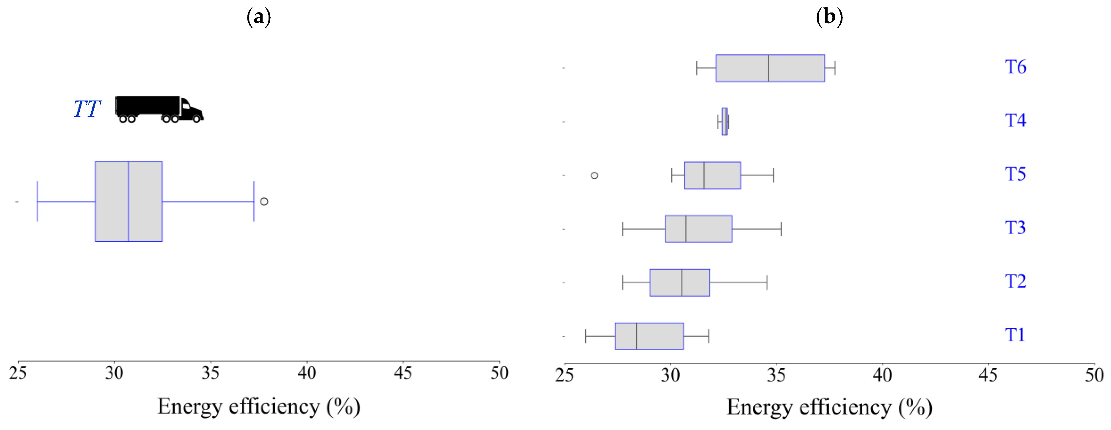
The establishment of energy efficiency benchmarks guides manufacturers and operators towards adopting greener technologies and practices. Based on the results obtained, energy efficiency standards can be established for the different vehicle categories. For example, for the case of the TT category, Figure 7a shows the energy efficiency distribution of all the TT vehicles included in this study. The quintiles define five groups of performance. Thus, technologies with energy efficiencies located in the first quintile (η < 28.40%) can be cataloged as red technologies, while technologies in the last quintile (η > 34.63%) can be classified as green or highly efficient technologies. The threshold values for the second and third quintiles are 30.52%, 31.58%, and 34.63%.

3.4. Main Drawbacks of the Proposed Method of Determining a Vehicle’s Energy Efficiency

For freight vehicles and heavy-duty passenger vehicles, accurately measuring payloads is essential for obtaining precise values of energy efficiency. Therefore, it is recommended that telematics systems include their own sensors to measure payloads. A sensitivity analysis showed that an error of 1 ton in a 54 GVWR produces a variation in energy efficiency of 0.8%, while an error of 100 kg in a 2 GVWR produces a variation of 1% in the obtained energy efficiency following the method proposed in Section 2.7.

This method does not promote the use of lighter vehicles because it includes the weight of the empty vehicle within the formula for determining energy efficiency.

The energy efficiency values obtained depend on the inertia equivalent mass (Equation (11)). Equation (11) is well accepted by the specialized community. However, we recommend conducting further research work to reconfirm its applicability to modern powertrain configurations, especially electric powertrains. Despite this, it remains a reliable method for estimating the energy efficiency of both conventional and electric vehicle powertrains.

4. Conclusions

This study demonstrates the feasibility of determining the energy efficiency of vehicles by monitoring their normal operational conditions (location, engine RPM, speed, payload, and fuel or energy consumption) at a frequency of 1 Hz. Currently, all these variables (except payload) can be monitored by telematic systems, which are often used in large fleets of heavy-duty vehicles.

The energy efficiency of a gasoline-fueled light-duty vehicle was tested on a chassis dynamometer and on the road in three cities under the same driving cycle. In all cases, the obtained energy efficiencies were not statistically different, demonstrating that the proposed method yields repeatable and reproducible results and produces values that are the same as those obtained through a well-accepted method involving a chassis dynamometer.

Similarly, energy efficiency was determined by applying the proposed method to samples of recent vehicle models of a single technology (diesel-fueled HDV) driven under normal conditions of use in three different countries. Despite the diversity of conditions of use, the observed energy efficiencies were not statistically different. This result confirmed that the proposed method yields repeatable and reproducible results. The results also demonstrated that the SFC (L/km) and SFC* (L/t-km) are not appropriate metrics for evaluating vehicle energy efficiency. The corresponding results are highly influenced by operational conditions.

Using the proposed method, energy efficiency was assessed across several vehicle types driven in México, Colombia, Ecuador, and Chile. It was found that electric vehicles exhibited the highest energy efficiency (73%), followed by diesel vehicles (27–35%). Gasoline-fueled vehicles exhibited the lowest energy efficiency (13–25%).

These findings demonstrate the applicability of the proposed method to determining energy efficiency. This method can be employed for each vehicle at a low cost. The results are independent of external factors (topography, weather conditions, and traffic) and human factors (driving style). However, its main drawback is the need for the actual weight of a vehicle, which is not currently included in telematics systems and, therefore, needs to be tracked by additional means.

The proposed method can be effectively applied to fleet renewal decisions, enabling fleet managers to make informed choices regarding vehicle replacements, optimize energy consumption, and reduce operational costs. Additionally, this approach offers a valuable tool for enhancing stakeholders’ operational efficiency by implementing more energy-efficient technologies in their fleets based on real performance data.

From a public policy perspective, these results provide reference values for establishing energy efficiency standards and guiding regulatory frameworks with which to drive technological advancement. The generated data can contribute to the development of regulations that promote the use of cleaner technologies, supporting the broader goal of reducing carbon emissions in the road transportation sector.

By implementing this method, fleet managers and policymakers can take actionable steps toward reducing fuel consumption, lowering operational costs, and contributing to the global effort to reduce the environmental impact of road transport.

References

- Fransen, T.; Welle, B.; Gorguinpour, C.; Mccall, M.; Song, R.; Tankou, A. Enhancing NDCs: Opportunities in Transport. 2019. Available online: www.wri.org/ (accessed on 24 June 2024).
- EAA. Reducing Greenhouse Gas Emissions from Heavy-Duty Vehicles in Europe; EAA: Oshkosh, WI, USA, 2022. [Google Scholar]
- IEA. World Energy Outlook 2024; IEA: Paris, France, 2024; Available online: https://www.iea.org/reports/world-energy-outlook-2024 (accessed on 18 November 2024).
- Fontaras, G.; Zacharof, N.G.; Ciuffo, B. Fuel consumption and CO2 emissions from passenger cars in Europe—Laboratory versus real-world emissions. Prog. Energy Combust. Sci. 2017, 60, 97–131. [Google Scholar] [CrossRef]
- Lohse-Busch, H.; Stutenberg, K.; Duoba, M.; Liu, X.; Elgowainy, A.; Wang, M.; Wallner, T.; Richard, B.; Christenson, M. Automotive fuel cell stack and system efficiency and fuel consumption based on vehicle testing on a chassis dynamometer at minus 18 °C to positive 35 °C temperatures. Int. J. Hydrogen Energy 2020, 45, 861–872. [Google Scholar] [CrossRef]
- SAE. Drive Quality Evaluation for Chassis Dynamometer Testing; SAE: Warrendale, PA, USA, 2014. [Google Scholar]
- Wang, B.; Pamminger, M.; Wallner, T. Impact of fuel and engine operating conditions on efficiency of a heavy duty truck engine running compression ignition mode using energy and exergy analysis. Appl. Energy 2019, 254, 113645. [Google Scholar] [CrossRef]
- Divekar, P.; Han, X.; Zhang, X.; Zheng, M.; Tjong, J. Energy efficiency improvements and CO2 emission reduction by CNG use in medium- and heavy-duty spark-ignition engines. Energy 2023, 263, 125769. [Google Scholar] [CrossRef]
- Zhu, Z.; Mu, Z.; Wei, Y.; Du, R.; Liu, S. Experimental evaluation of performance of heavy-duty SI pure methanol engine with EGR. Fuel 2022, 325, 124948. [Google Scholar] [CrossRef]
- Mulholland, E.; Ragon, P.-L.; Rodríguez, F. CO2 Emissions from Trucks in the European Union: An Analysis of the 2020 Reporting Period. Available online: https://theicct.org/wp-content/uploads/2023/07/hdv-co2-emissions-eu-2020-reporting-2-jul23.pdf (accessed on 9 August 2023).
- Li, H.; Khalfan, A.; Andrews, G. Determination of GHG emissions, fuel consumption and thermal efficiency for real world urban driving using a SI probe car. SAE Int. J. Engines 2014, 7, 1370–1381. [Google Scholar] [CrossRef]
- EC and JRC. VECTO Engine. 2018. Available online: https://climate.ec.europa.eu/document/download/76f0d05f-21cb-46f9-af06-e1f478fdccce_en?filename=201811_engine_en.pdf (accessed on 18 December 2023).
- EPA. Greenhouse Gas Emissions Model (GEM) User Guide: Vehicle Simulation Tool for Compliance with the Greenhouse Gas Emissions Standards and Fuel Efficiency Standards for Medium and Heavy-Duty Engines and Vehicles: Phase 2; EPA: Washington, DC, USA, 2016. [Google Scholar]
- Wang, C.; Yang, F.; Zhang, H.; Zhao, R.; Xu, Y. Energy recovery efficiency analysis of organic Rankine cycle system in vehicle engine under different road conditions. Energy Convers. Manag. 2020, 223, 113317. [Google Scholar] [CrossRef]
- Yadav, A.; Narla, A.; Delgado, O. Heavy-Duty Trucks in India: Technology Potential and Cost-Effectiveness of Fuel-Efficiency Technologies in the 2025–2030 Time Frame. 2023. Available online: https://theicct.org/wp-content/uploads/2023/06/India-HDT-fuel-efficiency_FINAL.pdf (accessed on 14 August 2023).
- DOE. DOE Announces $162 Million to Decarbonize Cars and Trucks. Available online: https://www.energy.gov/articles/doe-announces-162-million-decarbonize-cars-and-trucks (accessed on 12 July 2023).
- Abdurazzokov, U.; Sattivaldiev, B.; Khikmatov, R.; Ziyaeva, S. Method for assessing the energy efficiency of a vehicle taking into account the load under operating conditions. In E3S Web of Conferences; EDP Sciences: Les Ulis, France, 2021. [Google Scholar] [CrossRef]
- Casisi, M.; Pinamonti, P.; Reini, M. Increasing the energy efficiency of an internal combustion engine for ship propulsion with bottom ORCS. Appl. Sci. 2020, 10, 6919. [Google Scholar] [CrossRef]
- DOE. Vehicle Weight Classes & Categories; DOE: Washington, DC, USA, 2012. [Google Scholar]
- NTE INEN 2656; Clasificación Vehicular. INEN: Quito, Ecuador, 2016.
- MinTransporte. Resolución Número 20223040037985. 2022. Available online: https://mintransporte.gov.co/documentos/671/2022/?paginateDocs=100&genPagDocs=3 (accessed on 22 September 2023).
- Gutiérrez, J.; Gómez, N.; Chavarría, J. Análisis Estadístico para la Generación de Información Proveniente de Estaciones Dinámicas de Medición de pesos, Dimensiones y Velocidades Vehiculares para 2017. 2020. Available online: https://www.imt.mx/archivos/Publicaciones/PublicacionTecnica/pt605.pdf (accessed on 22 September 2023).
- TRANSPORTES. Decreto N° 122 de 1991; Ministerio de Transportes y Telecomunicaciones: Santiago, Chile, 2017. [Google Scholar]
- Pepper, G.T. Methods and System for Determining Consumption and Fuel Efficiency in Vehicles. U.S. Patent No. 7,774,130, 10 August 2010. [Google Scholar]
- Quirama, L.F.; Giraldo, M.; Huertas, J.I.; Jaller, M. Driving cycles that reproduce driving patterns, energy consumptions and tailpipe emissions. Transp. Res. D Transp. Environ. 2020, 82, 102294. [Google Scholar] [CrossRef]
- SAE. Fuel Consumption Test Procedure—Type II J1321_202010. 2020. Available online: https://www.sae.org/standards/content/j1321_202010 (accessed on 10 November 2023).
- Giraldo, M.; Restrepo, J.C.; Huertas, J.; Agudelo, J.R.; Agudelo, A.F. Signal synchronization methods when measuring tailpipe emissions with PEMS. Transp. Res. D Transp. Environ. 2024, 129, 104154. [Google Scholar] [CrossRef]
- Mustang Dynamometer. POWER DYNE PC Mustang Dynamometer Operator Manual. 2005. Available online: https://www.mustangdyne.com/wp-content/uploads/2020/09/Power-Dyne-PC-Users-Manual-v2017-05-22-01.pdf (accessed on 10 August 2024).
- UPME. Factores de Emisión de los Combustibles Colombianos (FECOC+) Fase I: Determinación de los Ciclos de Conducción de Fuentes Móviles de Carretera para Colombia. Available online: https://www1.upme.gov.co/DemandayEficiencia/Documents/Informe_final_FECOC.pdf (accessed on 26 June 2024).
- UPME. Factores de Emisión de los Combustibles Colombianos (FECOC+) Fase 2.2: Determinación de los Factores de Emisión de Vehículos Pesados de Carga (Camiones y Tractocamiones) y de Pasajeros (buses) a la Altitud de Bogotá y Barranquilla. Available online: https://www1.upme.gov.co/DemandayEficiencia/Doc_Hemeroteca/FECOC%2B2-2.pdf (accessed on 26 June 2024).
- Generadoras.cl. Generación Eléctrica en Chile. Available online: https://generadoras.cl/generacion-electrica-en-chile (accessed on 9 June 2024).
- Kelley Blue Book. What is MPGe? Everything You Need to Know. Available online: https://www.kbb.com/car-advice/what-is-mpge/#:~:text=What%20Does%20MPGe%20Mean%3F,electricity%20as%20its%20fuel%20source (accessed on 15 November 2023).
- UPME. Calculadora FECOC. 2016. Available online: https://app.upme.gov.co/Calculadora_Emisiones1/new/calculadora.html (accessed on 6 March 2024).
- INECC. Factores de Emisión para los Diferentes tipos de Combustibles Fósiles que se Consumen en México. Mexico City. 2014. Available online: http://www.inecc.gob.mx/descargas/cclimatico/2014_inf_parc_tipos_comb_fosiles.pdf (accessed on 10 November 2023).
- NTE INEN 935; Norma Técnica Ecuatoriana NTE INEN 935:2012, Derivados del Petróleo. Gasolina Requisitos (Octava Revisión). INEN: Quito, Ecuador, 2012.
- NTE INEN 1489; Norma Técnica Ecuatoriana NTE INEN 1489:2011 Derivados del Petróleo. Diesel Requisitos (Quinta Revisión). INEN: Quito, Ecuador, 2011.
- Huertas, J.I.; Serrano-Guevara, O.; Díaz-Ramírez, J.; Prato, D.; Tabares, L. Real vehicle fuel consumption in logistic corridors. Appl. Energy 2022, 314, 118921. [Google Scholar] [CrossRef]
- Gillespie, T.D. Fundamentals of Vehicle Dynamics—Revised Edition; SAE International: Warrendale, PA, USA, 2021. [Google Scholar]
- Albatayneh, A.; Assaf, M.N.; Alterman, D.; Jaradat, M. Comparison of the Overall Energy Efficiency for Internal Combustion Engine Vehicles and Electric Vehicles. Environ. Clim. Technol. 2020, 24, 669–680. [Google Scholar] [CrossRef]
Figure 1.
Methodology followed in this work to validate the proposed method for determining the real energy efficiency of vehicles. (a) Comparison of telemetry-based energy efficiency results with chassis dynamometer testing. (b) Methodology verification for a single technology under different conditions across three countries. (c) Energy efficiency evaluation of technologies in several Latin American countries. Acronyms: OR: on the road, M: vehicle mass (t), F: fuel use (L), Pos: position (lat: °, long: °, alt: masl), speed (km/h), PL: payload (t), WT: wheel torque (Nm), and WP: wheel power (kW).
Figure 2.
Altitude profile sample for normal-operation trips in (a) Ecuador and (b) Colombia, and speed–time profiles for (c–f) typical driving cycles in Colombia.
Figure 3.
Results regarding (a) SFC and (b) energy efficiency, observed in a single vehicle reproducing the same driving cycle on a chassis dynamometer and on the road at different altitudes.
Figure 4.
Fuel consumption and energy efficiencies observed among a sample of vehicles of the same make (International Prostar) under various operating conditions across different countries: (
a) specific fuel consumption (SFC), (
b) specific fuel consumption per payload (SFC*), and (
c) energy efficiency. DC: driving cycle displayed in
Figure 2f. NO: normal operating conditions described in
Section 2.4.
Figure 5.
Results regarding (a) SFC and (b) SFC* according to vehicle technology, categorized by vehicle type and test type. Relationship between total vehicle weight and (c) SFC, (d) SFC**, and (e) SFC*.
Figure 6.
Energy efficiency obtained for different vehicles in Chile, Colombia, México, and Ecuador in a driving cycle (DC) determined in on the-road-tests and on a chassis dynameter (dyno) and by monitoring their normal operating conditions (NO).
Figure 7.
Energy efficiency results for (a) the tractor-trailer (TT) category and (b) each TT.