Performance Analysis of a Rooftop Grid-Connected Photovoltaic System in North-Eastern India, Manipur

Abstract

The performance analysis of a 10 kW_p rooftop grid connected solar photovoltaic (PV) system located in Sagolband, Imphal, India has been studied for 5 years. The key technical parameters such as array yield ($Y_A$), reference yield ($Y_R$), final yield ($Y_F$), capacity utilization factor (CUF), PV system efficiency (${\eta }_{Sys}$), and performance ratio (PR) were used to investigate its performance. In this study, the experimentally measured results of the system’s performance for the five years (i.e., July 2018 to June 2023) were compared with the predicted results, which were obtained using PVsyst V7.3.0 software. The measured energy generation in 5 years (including 40 days OFF due to inverter failure on 17 June 2019 because of a surge, which was resolved on 27 July 2019) was 58,911.3 kWh as compared to the predicted 77,769 kWh. The measured daily average energy yield was 3.2 kWh/kW_p as compared to the predicted 4.2 kWh/kW_p. It can be seen that there was a large difference between the real and predicted values, which may be due to inverter downtime, local environmental variables (e.g., lower-than-expected solar irradiation and temperature impacts), and the possible degradation of photovoltaic modules over time. The measured daily average PR of the system was 70.71%, and the maximum occurred in the months of October, November, December, and January, which was almost similar to the predicted result. The measured daily average CUF of the system was 13.36%, and the maximum occurred in the months of March, April, and May. The measured daily average system efficiency was 11.31%. Moreover, the actual payback was 4 years and 10 months, indicating strong financial viability despite the system’s estimated lifespan of 25 years. This study highlights the importance of regular maintenance, fault detection, and better predictive modelling for more accurate energy projections, and also offers an understanding of real-world performance fluctuations.

1. Introduction

Ensuring energy security is an essential part of maintaining national security since energy is the building block of human civilization [1]. The substitution of non-fossil energy with renewable energy sources has emerged as a crucial component of the global energy supply system, aimed at mitigating environmental damage and fostering sustainable socio-economic growth [1,2]. The electricity produced by renewable energy sources, including hydropower, solar power, ocean power, wind power, etc., has been steadily expanding over the last decade. Solar energy is the most abundant renewable energy source on Earth compared to others, and it is accessible universally [3,4]. India has seen considerable progress in solar energy adoption, characterized by extensive photovoltaic installations and ambitious governmental efforts, like the National Solar Mission, which targets a solar power capacity of 100 GW by 2022 [4].

Assessing the performance of the photovoltaic system is crucial for analysis. This research is important for ascertaining the operational mechanisms of an efficient PV system. The performance of SPV systems has been studied and evaluated in several countries during the last few years [5,6,7,8,9]. The efficiency of a grid-connected PV system is contingent upon many factors, including cell technology, inverters, and installation arrangement. The outcome is also influenced by many meteorological factors, such as global irradiance, ambient temperature, and soiling losses [10,11]. A number of researchers have examined the economics and performance of grid-connected PV systems in various locations. Most of these studies, however, have limitations that include shorter monitoring times, limited reach in terms of real-world performance analysis, or dependence just on simulation-based findings. Sharma et al. [12] analyzed the performance of a 190 kW_p grid-interactive SPV power plant in India. They revealed that the plant obtained an average annual energy production of 812.76 kWh/kW_p and a system efficiency of 8.3%. Although this study provided useful insights into system efficiency, it lacked long-term monitoring, making it difficult to evaluate degradation trends over multiple years. Ashok et al. [13] investigated the performance of an on-grid PV system based on PVsyst modelling. However, this study primarily relied on simulation-based results without incorporating real-world operational issues such as inverter downtimes, seasonal variations, and grid instabilities. Rajesh et al. [14] proposed a technical performance investigation of a 186 kW_p grid-connected PV system. This revealed that the actual energy output agrees with the PVSyst and system advisor model predictions with an uncertainty of 1.34 percent. Despite this, the study did not explore the impact of long-term environmental conditions, such as soiling, temperature variations, or maintenance challenges, on the system’s efficiency. Using arrays made of polycrystalline silicon and copper indium selenide, both deployed at the same site, Ramanan et al. [15] carried out a comparative study of the efficiency of two grid-connected PV systems. The measured and projected results were evaluated in relation to the technology’s fit for Tamil Nadu’s hot and muggy climate. However, the study lacked an evaluation of the impact of extreme weather conditions on system performance and did not provide a detailed failure analysis. P. Ramanan et al. [16] analyzed the performance of a 1.25 kW_p grid-integrated SPV system operating in an outdoor setting. Similar to other studies, this work did not include detailed failure diagnostics, such as inverter breakdowns or unexpected system losses, which are essential for understanding real-world operational challenges. The 10 MWp connected grid installed on top of a canal was first commercialized in India, and Manish et al. [17], under actual field conditions, analyzed it quantitatively and qualitatively for performance and dependability. While the study covered large-scale installations, it did not provide a comprehensive comparison with small-scale rooftop PV systems, which have different efficiency constraints and economic considerations. Hassane et al. [18] conducted a performance study and examination of a 6 MW_p grid-connected PV system mounted in harsh desert environment conditions. Despite providing insights into large-scale systems, the study did not address issues such as panel degradation due to dust accumulation, inverter failures, or financial viability in different climatic zones. Bhogula et al. [19] performed a comprehensive evaluation of a 1 MW_p PV plant located at GITAM University, Andhra Pradesh, India. The evaluation included aspects such as the plant’s production and deterioration rate, as well as power and energy losses. However, it lacked a comparative assessment between predicted and actual performance over an extended period, limiting its applicability to long-term system evaluations. Ahmad et al. [20] presented the results of an inquiry into the data collected from a 467.2 kW_p PV system installed on the roofs of three high-rise buildings. While this study highlighted urban solar installations, it did not discuss small-scale residential systems or rooftop PV systems in subtropical and high-humidity regions. Based on the literature review, it was found that several studies have been conducted for performance analysis of solar PV system in different regions, but there is limited research on the performance of PV systems in regions with unique climate and geographical characteristics like those in Manipur. Therefore, the measurement of a photovoltaic system’s performance in Manipur is crucial due to the region’s distinctive meteorological and geographical characteristics, which considerably influence solar energy production. Manipur possesses a subtropical environment characterized by elevated humidity, substantial monsoonal precipitation, and fluctuating cloud cover, all of which can affect the performance and energy output of photovoltaic (PV) systems. Nonetheless, there is little research about the performance of PV systems in these conditions, which diverge from those in other parts of India. This study will yield critical data on the performance of photovoltaic systems in Manipur, facilitating the optimization of system design, maintenance, and energy output, thereby enhancing the sustainability and efficacy of solar energy solutions in the region. This research will address local energy requirements and enhance broader initiatives to promote renewable energy in comparable, under-explored regions.

To forecast how well a PV system would work at a particular site, you may choose from a variety of commercial software tools. In order to forecast the energy output of PV systems, these programs compile data from meteorological databases, PV modules, and inverters. The often-used PV simulation software available include PVsyst, system advisor model (SAM), PVSOL, and Helioscope, each of which has its advantages and drawbacks. Because of its well-known accuracy in performance prediction, large meteorological datasets, and ability to simulate real-world losses—including temperature impacts, soiling losses, and inverter efficiency—PVsyst V7.3.0 was selected for this study. For academic and commercial research, PVsyst is also a preferred choice since it provides strong energy yield estimates and financial modelling. PVsyst remains one of the most validated and extensively referenced tools in performance assessment studies of grid-connected PV systems, even while other programs like SAM provide thorough financial analysis and policy-related evaluations, and PVSOL offers improved visualization for small-scale rooftop systems. This research models the grid-connected system’s performance characteristics using the PVsyst simulation program. When it comes to studying, sizing, and analyzing data from whole PV systems, PVsyst is the software program to use. However, many studies relying on PVsyst do not incorporate real-world inefficiencies such as inverter failures, grid constraints, soiling losses, and maintenance issues, leading to over-optimistic performance predictions. A grid-connected PV system with a power output of 10 kW_p was extensively analyzed in this study for the moderate climatic condition of Manipur, looking at both its actual and predicted performance. We compared the accurately measured performance parameters with the parameters simulated using PVsyst software under various resource datasets. The data were collected for a period of five years, from 1 July 2018 to 30 June 2023. Simulations were conducted utilizing climatic data obtained from measurements, as well as data provided by NASA POWER Data Access Viewer (DAV) V2.4.14. The performance characteristics that were studied include yearly energy produced, performance ratio, final yield, and reference yield. The acquired findings provide valuable information on the PV system’s performance, as well as the reliability of employing both measured and calculated meteorological data in Sagolband, Imphal, India. Finally, we compared our findings to those of other research conducted on a global scale.

The remainder of this paper is arranged as follows: The SPV system description is presented in Section 2. Section 3 discusses the technical performance parameters of the PV systems. The results and discussion are explained in Section 4. In Section 5, the conclusion is presented.

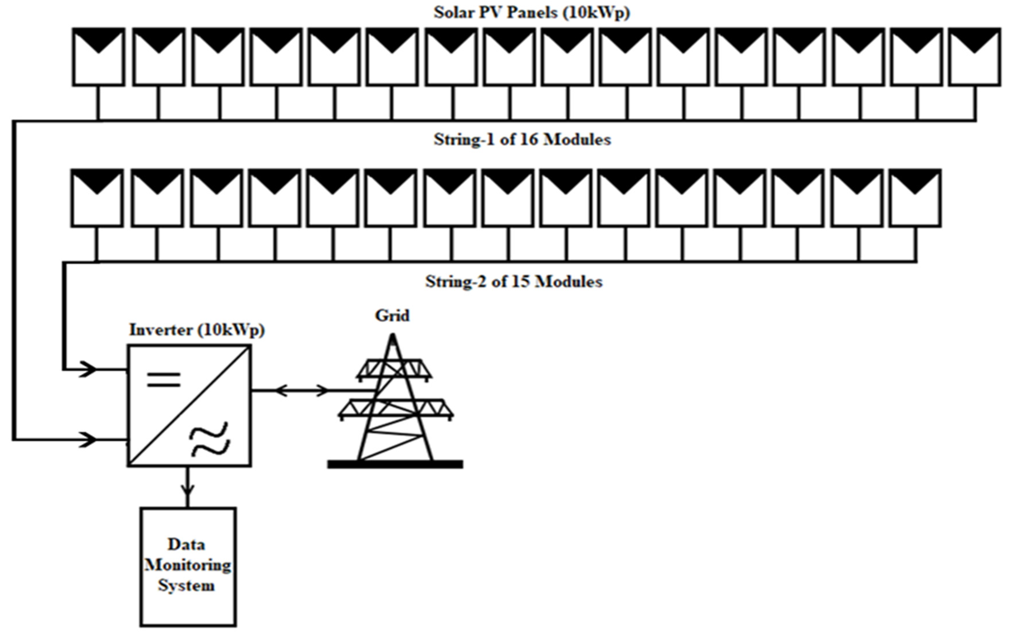
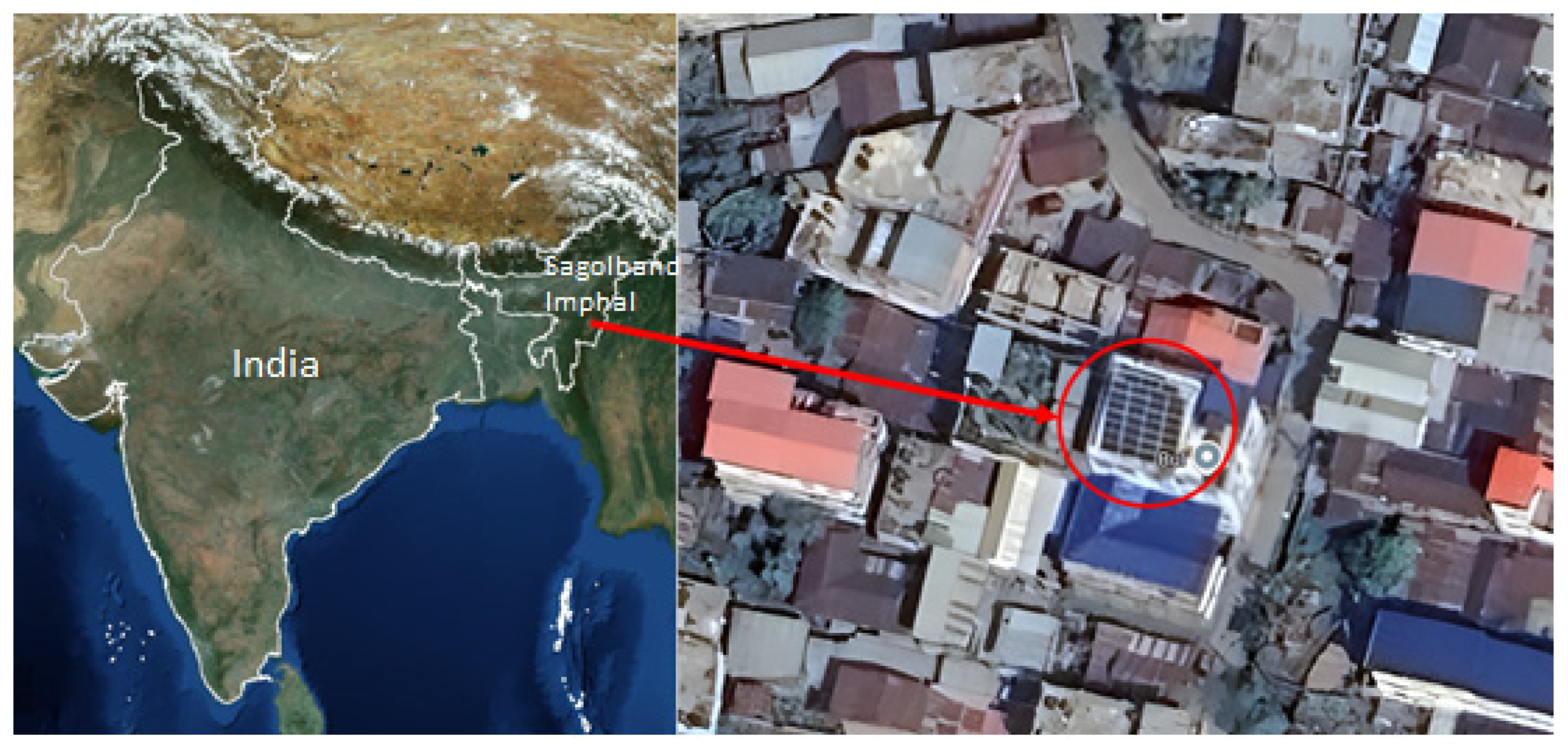
2. PV System Description

The PV system was installed on the terrace of the fourth floor of a building, which was 15 m above ground level at Sagolband, Imphal (24.804° N, 93.926° E). The system consisted of 31 poly-crystalline modules and had two strings. One string connected 16 modules in series, and the other string 15 modules in series. The system faced South at a fixed tilt angle of 22° and an azimuth angle of 0°.

DC was converted to AC and sent straight to the power grid using a 3-phase ABB solar inverter 10 kW on a grid with two separate MPPTs using RS-485 (communication interface), with 10.3 kW rated as DC input power and 10 kW rated as AC output power.

The monitoring period for the present study was 5 years, from July 2018 to June 2023. The values of GHI, DHI, ambient temperature, and clearness index were taken as daily averages. The energy generated by the grid was monitored online every hour using a data logger. The site details of the installed 10 kW_p rooftop grid-connected PV system are given in

Table 1. Site details of the installed 10 kW_p rooftop grid-connected PV system.

Site	State, Country	Latitude at the Site	Longitude at the Site	Inclination of the Panel	Region
Sagolband, Imphal	Manipur, India	+24.804° N	+93.926° E	22°	North-eastern part of India

. The specifications of the 10 kW_p rooftop Grid-connected PV system are given in

Table 2. Specifications of 10 kW_p rooftop Grid-connected PV system.

System	Manufacturer and Name	Specifications
PV Panel	Alpex company (Greater Noida, India) (ALP325W)	Type of modules = poly-crystalline, PoweRated (PR) = 325 Wp, Vmp = 37.67 V, Imp = 8.63 A, VOC = 45.41 V, ISC = 9.34 A, efficiency (ηp) = 16.34%, no. of modules = 31, no. of module string = 2, module tilt = 22°, area of each panel (Ap) = 1.99 m2
Inverter	ABB (Zürich, Switzerland) (PVI-10.0-TL-OUTD 10 kW)	Three-phase string inverter, 10 kWac, 2MPPT, RS-485 communication interface. Rated DC input power (Vdcr) = 10.3 kW, maximum DC input power for each MPPT = 6500 W, maximum DC input current for each MPPT = 17 A, rated AC output power = 10 kW, rated AC grid voltage = 400 V, rated efficiency = 97%, communication interface was WLAN

. Figure 1 shows the system’s schematic drawing. Figure 2 shows the projected PV system’s Google Maps image.

3. Technical Performance Parameters of the PV Systems and PVsyst Configuration for Simulation

In accordance with the International Energy Agency (IEA), the 10 kW_p grid-connected PV system’s performance was examined [21].

Table 3. Technical parameters of PV system.

Sl. No.	References	Performance Indices	Definitions	Expression	Equation No.
1.	[22]	Reference yield ($Y_R$)	Total in-plane irradiance, $G_i$ divided by solar radiation under standard test conditions.	$Y_R={\displaystyle \frac{G_i}{G_{STC}}}$	(1)
2.	[23]	Array Yield (YA)	Energy produced by the array.	$Y_A={\displaystyle \frac{E_{DC,d}}{P_{PV,rated}}}$	(2)
3.	[23]	Final Yield ( $Y_F)$	Energy fed to the grid.	$Y_F={\displaystyle \frac{E_{AC,d}}{P_{PV,rated}}}$	(3)
4.	[24]	System efficiency $\left({\eta }_{sys}\right)$	Input GHI to energy fed to the grid.	${\eta }_{sys}=\left({\displaystyle \frac{E_{AC, d}}{H_t{A}_a}}\right)\times 100\%$	(4)
5.	[25]	Performance ratio (PR)	Energy generated to grid with regard to installed capacity of PV system.	$\mathrm{PR}={\displaystyle \frac{Y_F}{Y_R}}\times 100(\%)$	(5)
6.	[26]	Capture loss ( $L_C)$	Loss in PV panel in conversion from GHI to electricity.	$L_C=Y_R-Y_A$	(6)
7.	[26]	System loss ( $L_s)$	Losses due to inverter and wiring material	$L_s=Y_A-Y_F$	(7)
8.	[27]	Capacity utilization factor (CUF)	The PV plant’s actual energy production for an entire year, 24 h a day, compared to the maximum energy generation of rated power during that time.	$\mathrm{CUF}={\displaystyle \frac{Y_{F,a}}{24\times 365}}$	(8)

G_STC = Solar irradiation under standard test conditions (STCs) (kWh/m²/day), P_PVrated = PV array capacity (kW_p), Aa = PV array area (m²), E_{DC, d} = daily PV array output (kWh/kW_p), E_AC,d = daily energy to grid (kWh/kW_p), Y_F,a = annual final yield, and G_i = total in-plane irradiance (kWh/m²/day).

shows the several parameters used in the analysis.

The PVsyst was set with particular system settings to ensure a precise simulation of the installed PV system. For solar radiation, temperature, and wind speed, the simulation utilized NASA POWER Data Access Viewer’s meteorological data. The actual PV array, together with module type, rated power, temperature coefficient, and degradation rates, determined the module parameters. Also, the inverter settings were aligned with the system that was installed, taking into account the efficiency curves, the maximum power point tracking (MPPT) range, and the inverter losses.

Loss parameters were also adjusted to represent real-world scenarios, including temperature losses, mismatch losses, wire losses, and inverter losses, depending on seasonal accumulation patterns. With no tracking, the tilt angle and azimuth were set based on the fixed installation of the system in Manipur. Grid availability was taken into account to adjust for any potential disruptions. These configurations ensured that the simulated results closely matched real-world conditions while identifying discrepancies between modelled and measured energy output.

4. Results and Discussions

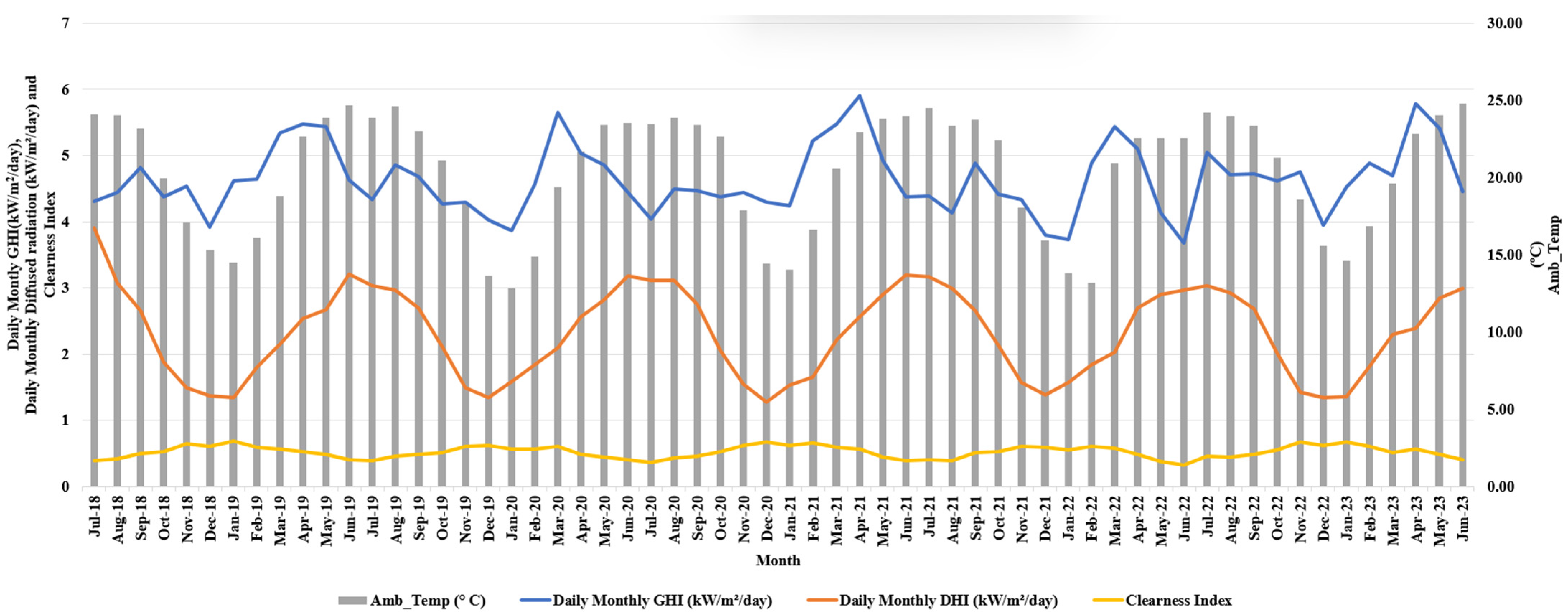
4.1. Metrological Site

This study of the PV system was conducted over five years (July 2018–June 2023), and the metro data, such as GHI, DHI, amb-temp, and clearness index, were recorded from NASA metrological data for every hour interval. The data were taken from the NASA POWER network’s database, which can be found at NASA POWER Data Access Viewer. Accessing the dataset under the “Renewable Energy” category for Sagolband, Imphal, India’s study site’s geographical coordinates—22° N, 93.926° E—were used. The variation in daily monthly GHI, DHI, ambient temperature, and clearness index from July 2018 to June 2023 is depicted in Figure 3. The monthly average data varied during these five years, which is given below, and the maximum and minimum values of each year are also presented in

Table 4. Variation in daily monthly GHI, DHI, Amb_Temp, and clearness index.

Parameters	July 2018–June 2019	July 2019–June 2020	July 2020–June 2021	July 2021–June 2022	July 2022–June 2023
GHI (kW/m2/day)	April 19—5.47 (Max) Dec 18—3.92 (Min)	March 20—5.65 (Max) Jan 20—3.87 (Min)	April 21—5.9 (Max) Jul 20—4.04 (Min)	March 22—5.43 (Max) Jun 22—3.68 (Min)	April 23—5.79 (Max) Dec 22—3.95 (Min)
DHI (kW/m2/day)	Jul 18—3.91 (Max) Jan 19—1.34 (Min)	Jun 20—3.18 (Max) Dec 19—1.35 (Min)	Jun 21—3.19 (Max) Dec 20—1.28 (Min)	Jul 21—3.17 (Max) Dec 21—1.39 (Min)	Jul 22—3.03 (Max) Dec 22—1.35 (Min)
Amb_temp (°C)	Jun 19—24.65 (Max) Jan 19—14.49 (Min)	Aug 19—24.61 (Max) Jan 20—12.85 (Min)	Jun 21—24 (Max) Jan 21—14.06 (Min)	Jul 21—24.52 (Max) Feb 22 13.18 (Min)	Jun 23—24.82 (Max) Jan 23—14.59 (MIN)
Clearness Index	Jan 19—0.68 (Max) July 18—0.39 (Min)	Dec 19—0.62 (Max) Jul 19—0.39 (Min)	Dec 20—0.67 (Max) Jul 20—0.37 (Min)	Nov 21, Feb 22—0.61 (Max) Jun 22—0.33 (Min)	Nov 22, Jan 23—0.67 (Max) Jun 23—0.40 (Min)

.

(a)

GHI ranged from 3.68 (June 2022) to 5.78 kW/m²/day (April 2023).

(b)

DHI ranged from 1.28 (December 20220) to 3.19 kW/m²/day (July 2018).

(c)

Ambient temperature ranged from 12.85 °C (January 2020) to 24.82 °C (June 2023).

(d)

Clearness index ranged from 0.33 (June 2022) to 0.68 (January 2019).

When analyzing the performance of a solar PV system, it is essential to take into account accurate environmental data, including solar irradiance, temperature, and shading effects. However, errors in this data may lead to inaccurate measurements or simulations, affecting the system’s performance. Discrepancies may also be introduced by instrumental errors, such as problems with calibrating pyranometers, temperature sensors, or voltage/current meters. System performance differences over time may sometimes go unrecognized due to data sampling frequency and precision issues. Predictions of simulation performance could be off because the assumptions about system efficiency, inverter losses, and degradation rates do not always match reality. Moreover, discrepancies in measured and simulated data might be caused by differences in panel orientation, installation circumstances, and maintenance methods.

Figure 3 shows that for the last five years, the highest amount of diffused radiation occurred during the monsoon season. (i.e., June, July, and August). Diffusion of radiation was lowest in the winter months of November, December, and January throughout the five years. Over five years, the clearness index ranged from 0.33 to 0.68. The November, December, and January months had the clearest index, while June and July had the cloudiest. Moreover, it was also found that the months with the highest levels of diffused radiation also had the lowest clearness index readings. In the same way, the months with the lowest dispersed radiation and the highest clearness index were the same. The connection between these two variables shows that the most diffused radiation happens when the sky is cloudy, and the least diffused radiation happens when the sky is clear.

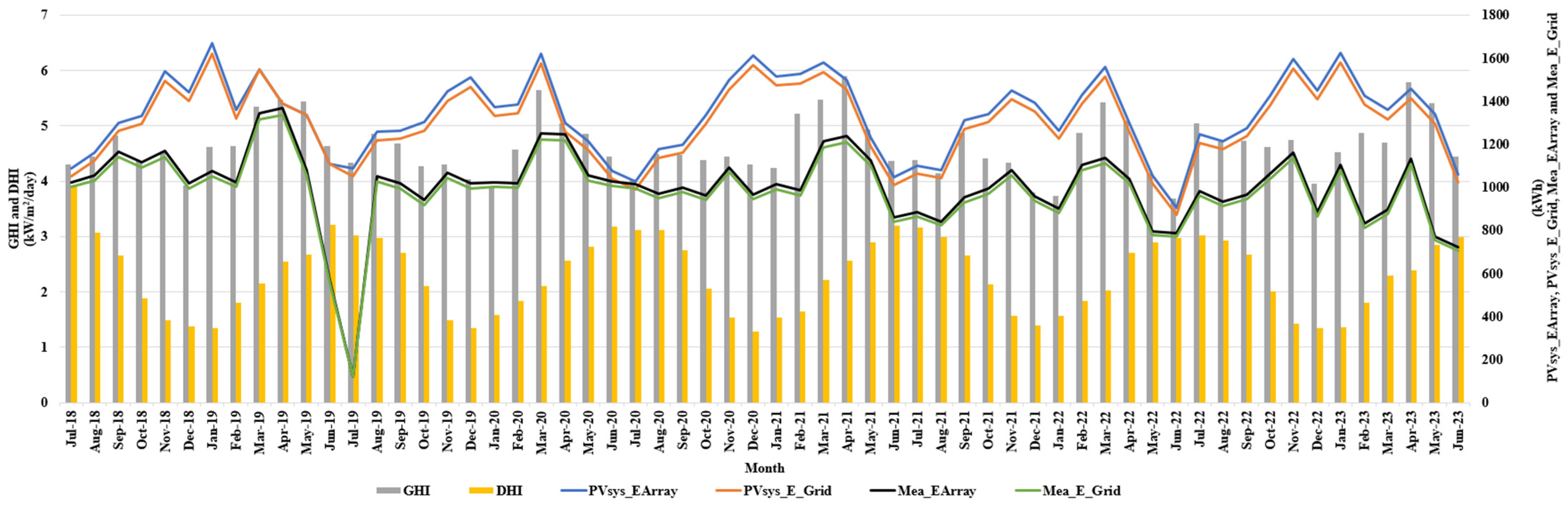
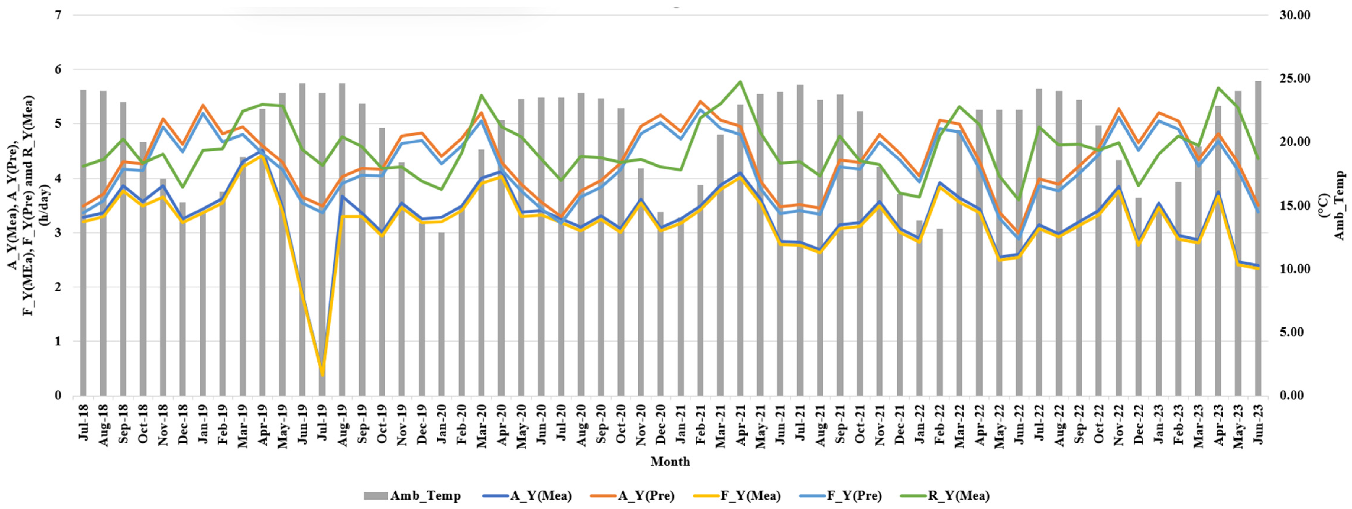
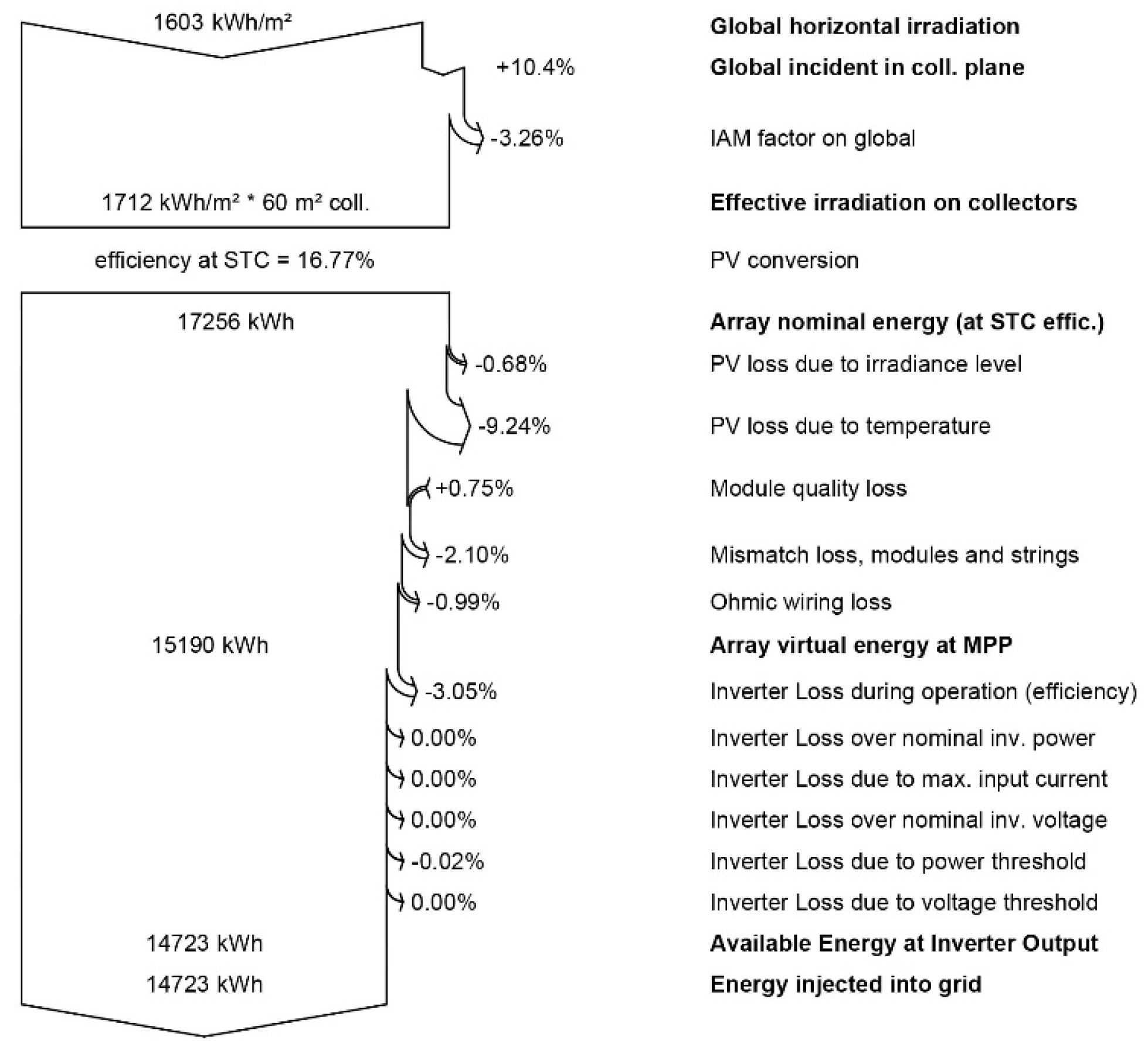
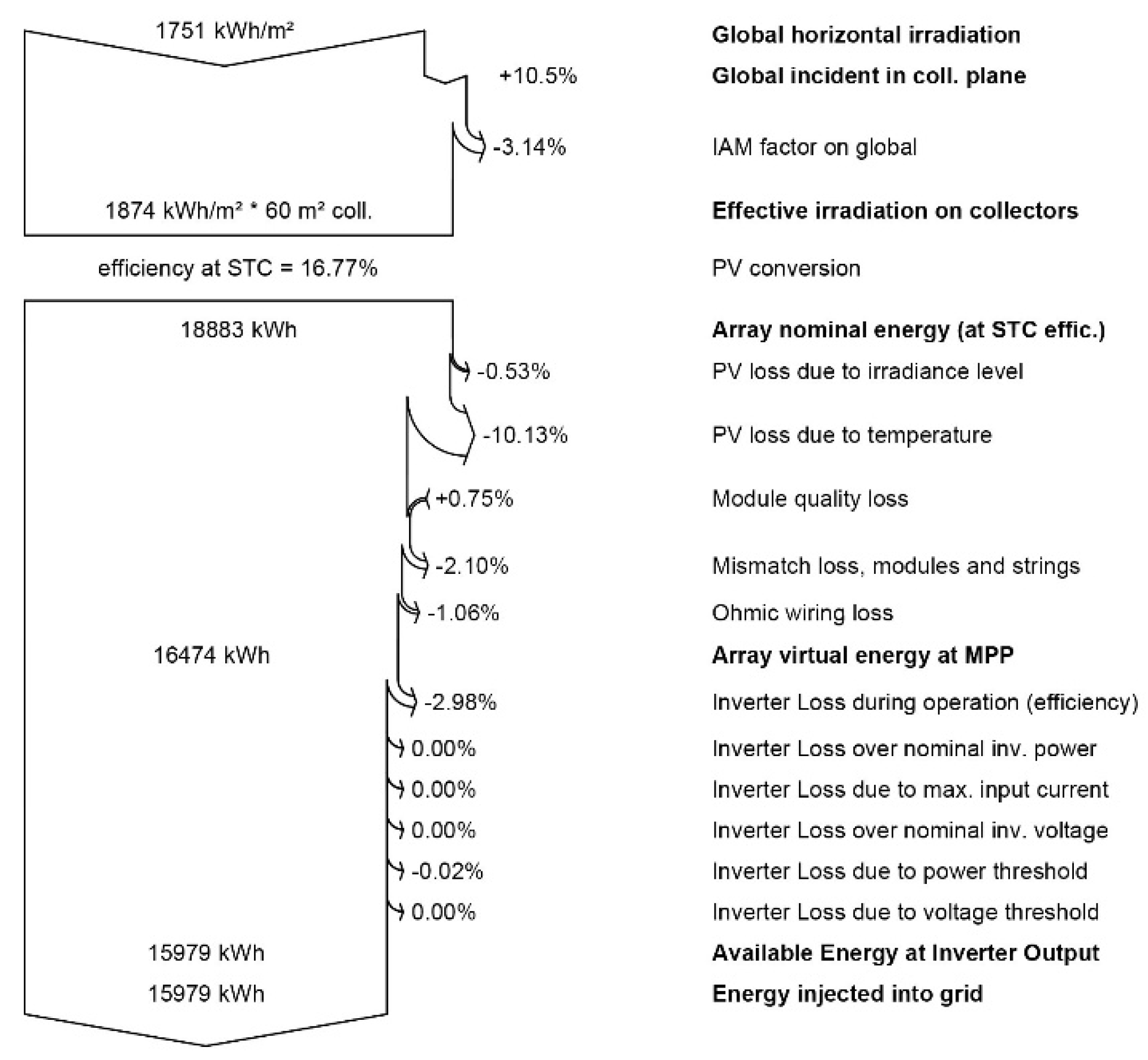
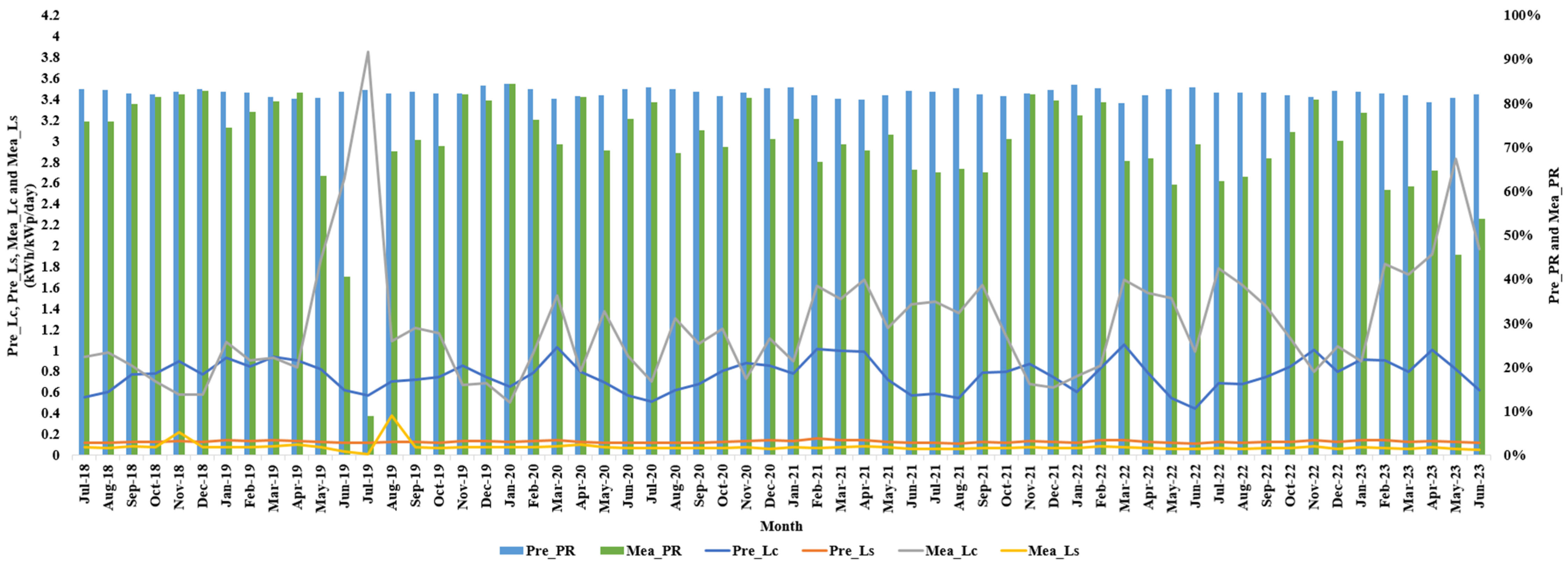
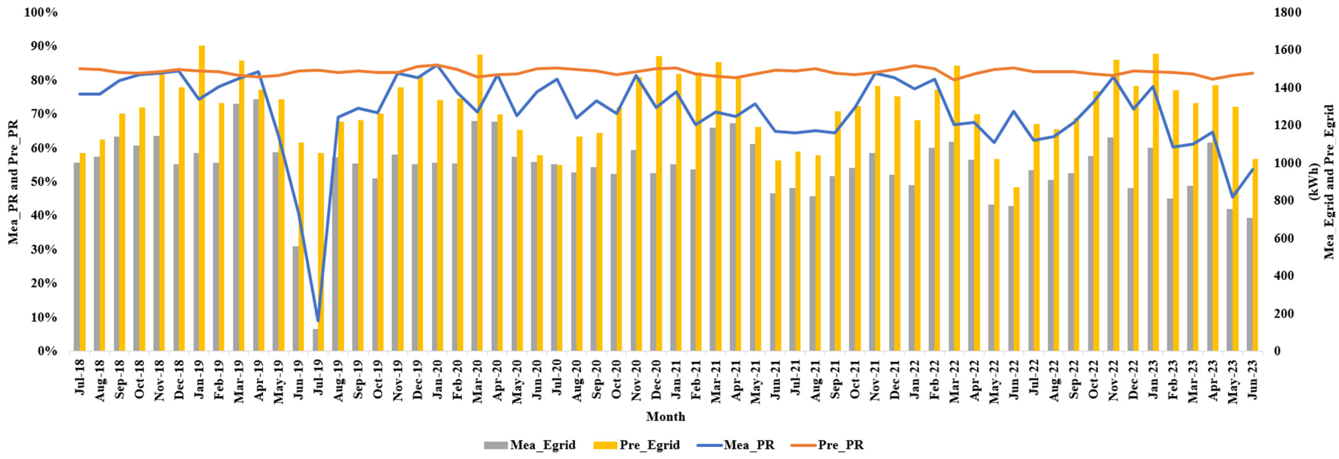
4.2. Energy Variation Analysis

Figure 4 shows the monthly energy production observed and forecasted based on GHI and DHI for five years. Figure 5 illustrates the monthly differences between predicted and measured array yield, final yield in relation to reference yield, and ambient temperature. Where PVsys_EArray, PVsys_E_Grid, Mea_EArray, and Mea_E_Grid represent Predicted power at the solar panel, predicted power directly given to the grid, i.e., the output of the inverter to the grid, measured power at the solar panel and measured power directly given to the grid, i.e., the output of the inverter to the grid, respectively. The annual energy variation analysis of these five years is discussed below.

In the first year, from July 2018 to June 2019, the measured monthly highest energy generation was in April 2019, followed by the months of March 2019 and November 2018, which were also closely related to the predicted E-grid results, as shown in Figure 4. The measured least generation was in June 2019 (because on 17 June 2019, the inverter was damaged due to a surge and given to the company for repair), followed by December 2018, which had the minimum GHI of the year (i.e., 3.92 kW/m²/day) and was also slightly low compared to the predicted. The maximum diffuse radiation was obtained in July 2018, while the minimum diffuse radiation was obtained in Jan 2019. As illustrated in Figure 5, the highest recorded ambient temperature happened in June 2019, while the lowest recorded temperature happened in January 2019. Again, Figure 5 shows that the measured final yield was maximum in April 2019, and its ambient temperature was 22.64 °C; the measured minimum energy generation was in June 2019 with an ambient temperature of 24.65 °C and, again, Figure 5 also shows that the expected array yield and final yield at the time of high energy generation were also rather near to the measured array and final yield.

In the second year (i.e., July 2019–June 2020), the monthly highest energy generation was measured in March 2020, followed by April 2020, which was also closely related to the predicted E-grid results, as shown in Figure 4. The measured least generation was in July 2019 (because on 17 June 2019, the inverter was damaged due to a surge and given to the company for repair, and it was resolved on 27 July 2019), followed by October 2019, which was the GHI (i.e., 4.27 kW/m²/day) and was also slightly low compared to the predicted. The maximum diffuse radiation was obtained in June 2020, while the minimum diffuse radiation was obtained in Dec 2019, as shown in Figure 4. The maximum ambient temperature was obtained in August 2019, while the minimum ambient temperature was obtained in January 2020, as shown in Figure 5. The measured final yield was at its maximum in the month of April 2020, and its ambient temperature was 21.70 °C. The measured minimum final yield was in the month of July 2019, and its ambient temperature was 23.86 °C, as shown in Figure 5. The predicted array yield and final yield were also close to the measured array and final yield at the time of high energy generation, as shown in Figure 5.

In the third year (i.e., July 2020–June 2021), the measured monthly highest energy generation was in April 2021, followed by the months of March 2021 and May 2021, which were also closely related to the predicted E-grid results, as shown in Figure 4. The measured least generation was in June 2021, which had the GHI (i.e., 4.37 kW/m²/day) and was also slightly low compared to the predicted. The maximum diffuse radiation was obtained in Jun 2021, while the minimum diffuse radiation was obtained in Dec 2020. Figure 5 shows the ranges of the ambient temperature: 14.49 °C to 22.65 °C. June 2021 had the highest ambient temperature; January 2021 had the lowest ambient temperature. The measured final yield was maximum in the month of April 2021, and its ambient temperature was 22.97 °C. The measured minimum energy generation was in the month of June 2021, and its ambient temperature was 24 °C, as shown in Figure 5. The predicted array yield and final yield were also close to the measured array and final yield at the time of high energy generation, as shown in Figure 5.

In the fourth year (i.e., July 2021–June 2022), the measured monthly highest energy generation was in March 2022, followed by the months of Feb 2022 and April 2022, which were also closely related to the predicted E-grid results, as shown in Figure 4. The measured least generation was in June 2022, which had the minimum GHI of the year (i.e., 3.68 kW/m²/day) and was also slightly low compared to the predicted. The maximum diffuse radiation was obtained in July 2021, while the minimum diffuse radiation was obtained in Dec 2021. The maximum ambient temperature was obtained in July 2021, while the minimum ambient temperature was obtained in Feb 2022, as shown in Figure 5. The measured final yield was maximum in the month of Feb 2022, and its ambient temperature was 13.18 °C, and the measured final yield was minimum in the month of May 2022, and its ambient temperature was 22.54 °C, as shown in Figure 5. The predicted array yield and final yield were also close to the measured array and final yield at the time of high energy generation, as shown in Figure 5.

In the fifth year (July 2022–June 2023), the measured monthly highest energy generation was in Nov 2022, followed by the months of Jan 2023 and April 2023, which were also closely related to the predicted E-grid results, shown in Figure 4. The measured least generation was in June 2023, which had the GHI (i.e., 4.45 kW/m²/day) and was also slightly low compared to the predicted. The maximum diffuse radiation was obtained in July 2022, while the minimum diffuse radiation was obtained in Dec 2022. The maximum ambient temperature was obtained in June 2023, while the minimum ambient temperature was obtained in Jan 2023, as shown in Figure 5. The measured final yield was maximum in the month of Nov 2022, and its ambient temperature was 18.57 °C, and the measured final yield was minimum in the month of June 2023, and its ambient temperature was 24.82 °C, as shown in Figure 5. The predicted array yield and final yield were also close to the measured array and final yield at the time of high energy generation, as shown in Figure 5.

The summary of the energy variation analysis of these five years is discussed below: (a) During the period of 5 years from July 2018 to June 2023, the measured energy generation varied from July 2019 (i.e., 119 kWh) to April 2019 (i.e., 1337.6 kWh), while the monthly average value was 981.85 kWh, as shown in Figure 4. It was found that the measured minimum energy generation value (i.e., 119 kWh) was quite small compared to the predicted value (i.e., 905 kWh) because the inverter failed on 17 June 2019 due to a surge; otherwise, the measured value would be almost similar with the predicted result. (b) The highest GHI was obtained in April 2021 (i.e., 5.9 kW/m²/day), while the lowest was obtained in June 2022 (i.e., 3.68 kW/m²/day). (c) The maximum diffuse radiation was obtained in July 2018 (i.e., 3.91 kWh/m²/day), while the minimum diffuse radiation was obtained in Dec 2020 (i.e., 1.28 kWh/m²/day). (d) The highest measured final yield was obtained in April 2019 (i.e., 4.42 h/day), while the lowest final yield was obtained in July 2019 (i.e., 0.38 h/day), as shown in Figure 5. The measured average final yield was found to be 3.20 h/day, which was better compared to many locations, as presented in

Table 5. Performance evaluation of several grid-connected solar PV systems.

Location	Panel Type	Capacity (KWp)	Monitoring Period (Year)	Annual AC Generation (MWh)	Final Yield (h/day)	PV Efficiency (%)	CUF	PR (%)	References
Bhubaneswar, India	P-Si	11.2	1	14.96	3.67	1 × 3.42	15.27	78	[28]
Vasant Kunj, New Delhi	PC	48	1	59.58	3.14	11.95	13.9	80	[29]
Bhel, Tiruchirappalli, Tamil Nadu	p-Si	20	1	30.14	-	-	17.2	82	[25]
Integral University, Lucknow	p-Si	467.2	3	1911.5	-	15.47	15.25	80.86	[20]
Khatkar-Kalan, India	p-Si	190	1	154.42	2.33	8.3	9.27	74	[12]
Thuvakudi, Tiruchirappalli, India	MC-Si A-SI PC-Si	5	1	8495.3	4.81	5.08	-	89	[30]
Bahir Dar, Ethiopia	Mono-Crystalline	10	1	11.81	2.02–3.45	9.3–10.7	-	64.74	[31]
Dublin, Ireland	Mc-Si	13	3	-	1.69	6.4	-	60–62	[32]
IIT, Roorkee, India	P-Si	1816	1	2.203	3.32	8.7	13.85	63.68	[33]
University of Lucknow, India	-	5	1	7.175	3.99	10.02	16.39	76.97	[26]
Wellington, New Zealand	Monocrystalline	10	1	-	2.99	11.96	12.5	78	[34]
Amity University, Haryana, India	Multi-Crystallin	186	1	289.391	4.28	13.76	17.8	82.7	[13]
Karnataka, India	Mono-crystallin	3000	1	4204	3.75	12.3	20	70	[35]
Sagolband, Imphal, Manipur, India	P-Si	10	5	58.911	3.20	11.31	13.36	70.71	Present Study

.

Since several factors (like shade, dust accumulation, cloud cover, inverter performance, etc.) influence PV performance, not only sunlight levels, but also reference yield and energy production prediction from PVsyst did not quite match the GHI profile. More energy generation normally results from higher GHI high temperatures during the April–June peak solar months, which affect panel efficiency, so it produced less than predicted energy output. The variations in these aspects also came from other elements such as shade, dust accumulation, cloud cover, and inverter performance.

In general, inverter failures, changes in weather conditions, temperature-induced efficiency losses, and panel degradation account for most of the difference between the expected and measured energy generation during the five years. The June 2019 inverter failure had a long-lasting effect that clearly reduced energy generation in the next year. Also, the PVsyst model assumed a constant cleaning schedule that did not reflect actual conditions or soiling losses, especially in the dry months, which partially explains the lower than expected efficiency. The variations in actual rather than modelled meteorological data, especially those in GHI and ambient temperature, caused variation from the intended performance. Temperature impacts were also quite important; high ambient temperatures caused thermal losses that were not entirely reflected in the PVsyst’s default settings. Furthermore, in the later years, PV module deterioration became more important and influenced system efficiency more than the conventional linear degradation assumption applied in PVsyst. PVsyst modelling should combine real-time weather data, a more dynamic degradation model based on the actual panel performance, and a better estimation of soiling losses to raise prediction accuracy and increase system performance. Passive cooling systems and better inverter protection mechanisms might increase the general reliability of the system, and also regular maintenance measures, which include automatic soiling detection and optimal cleaning schedules, could help reduce efficiency losses.

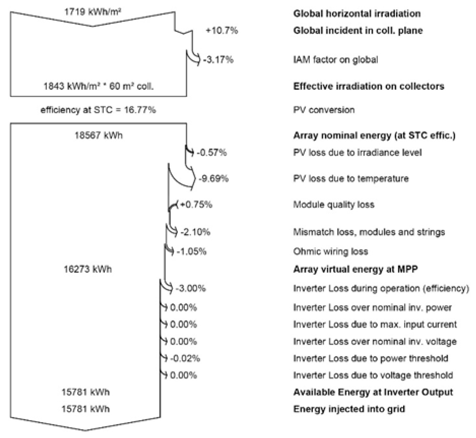
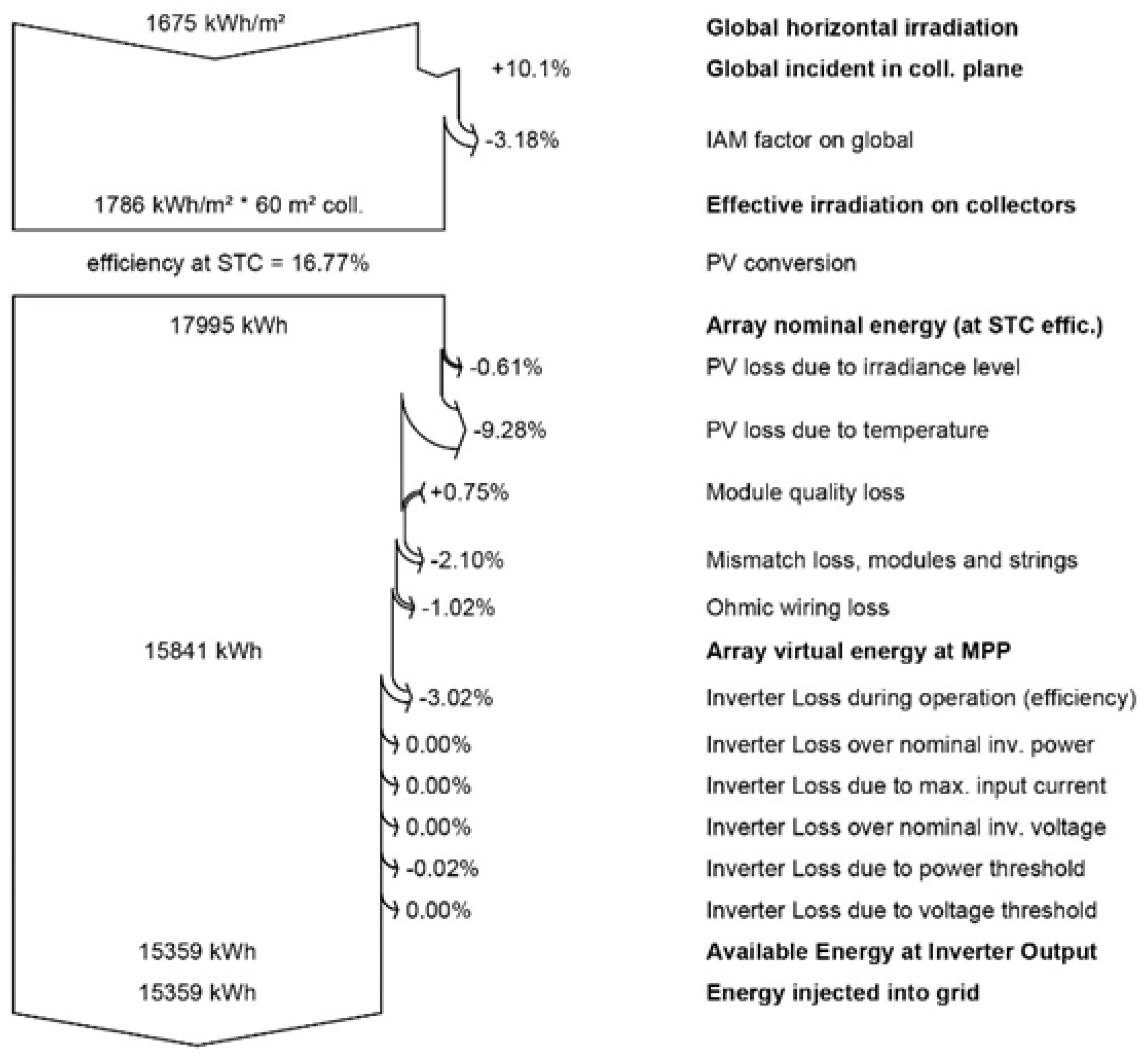
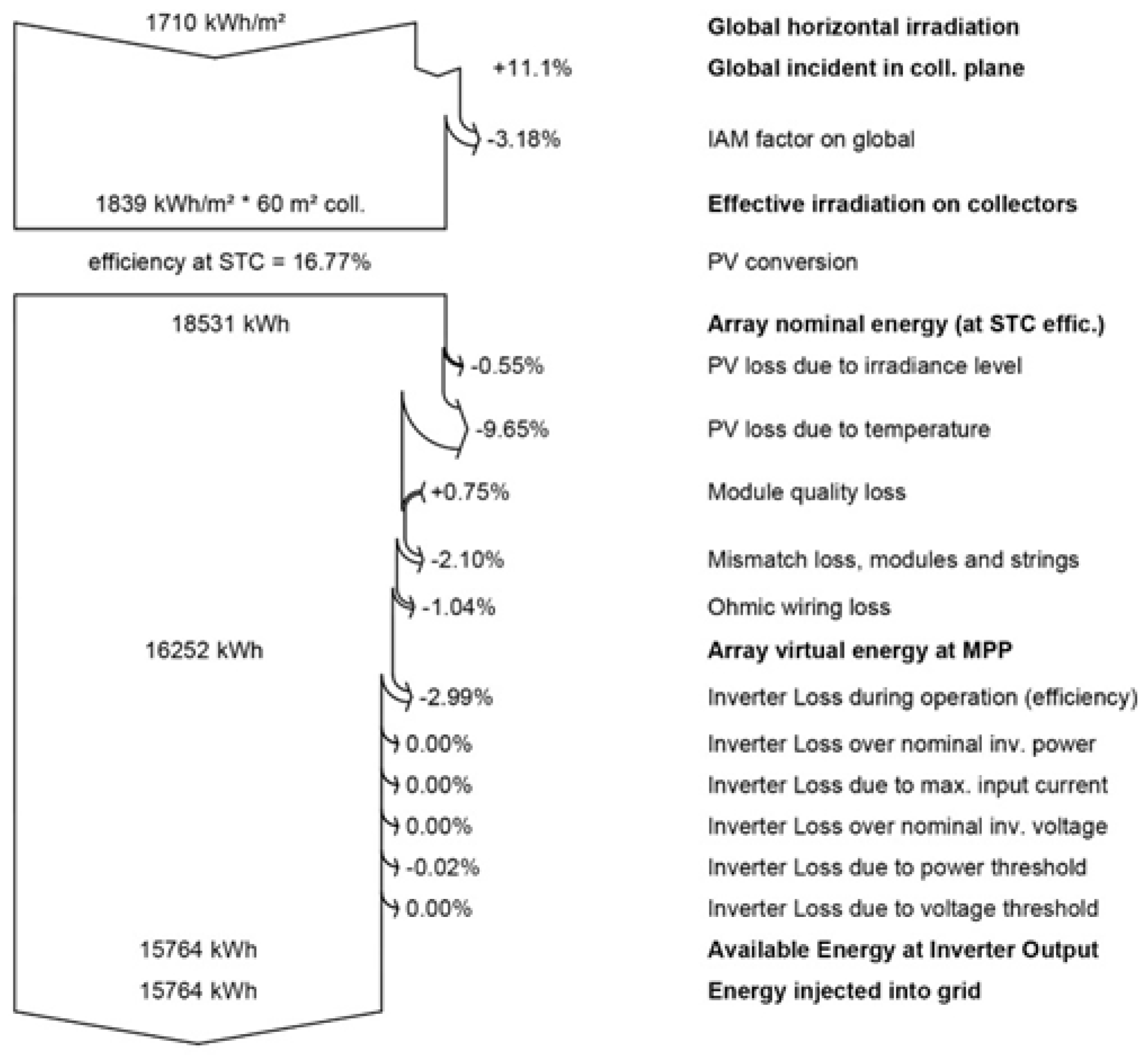
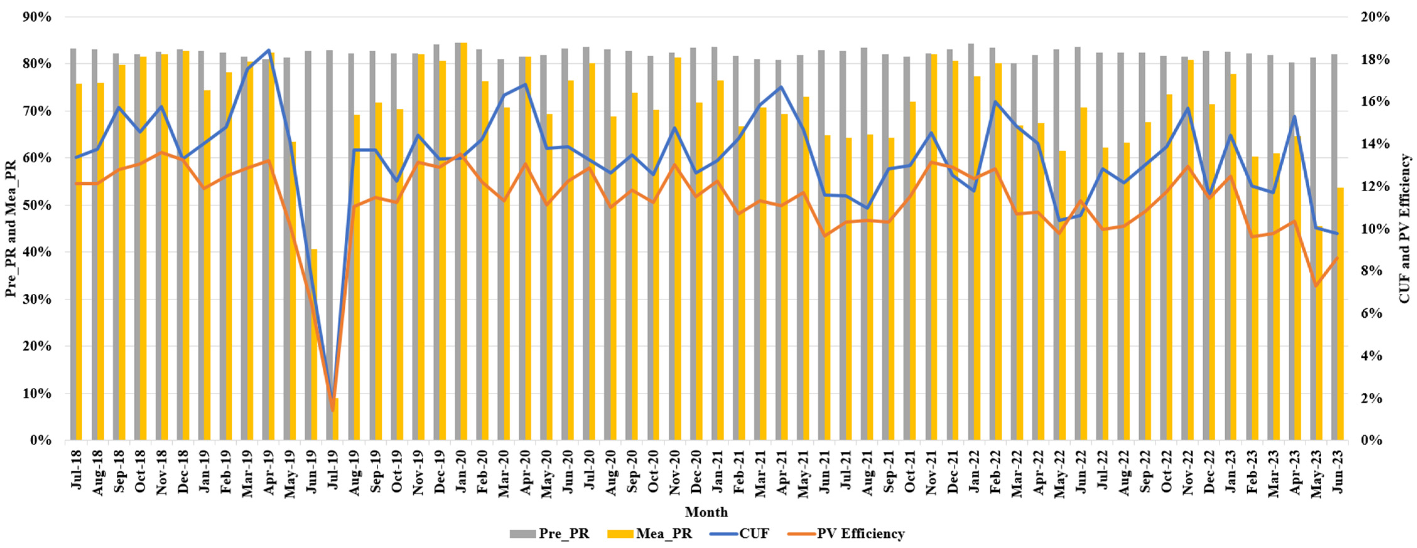
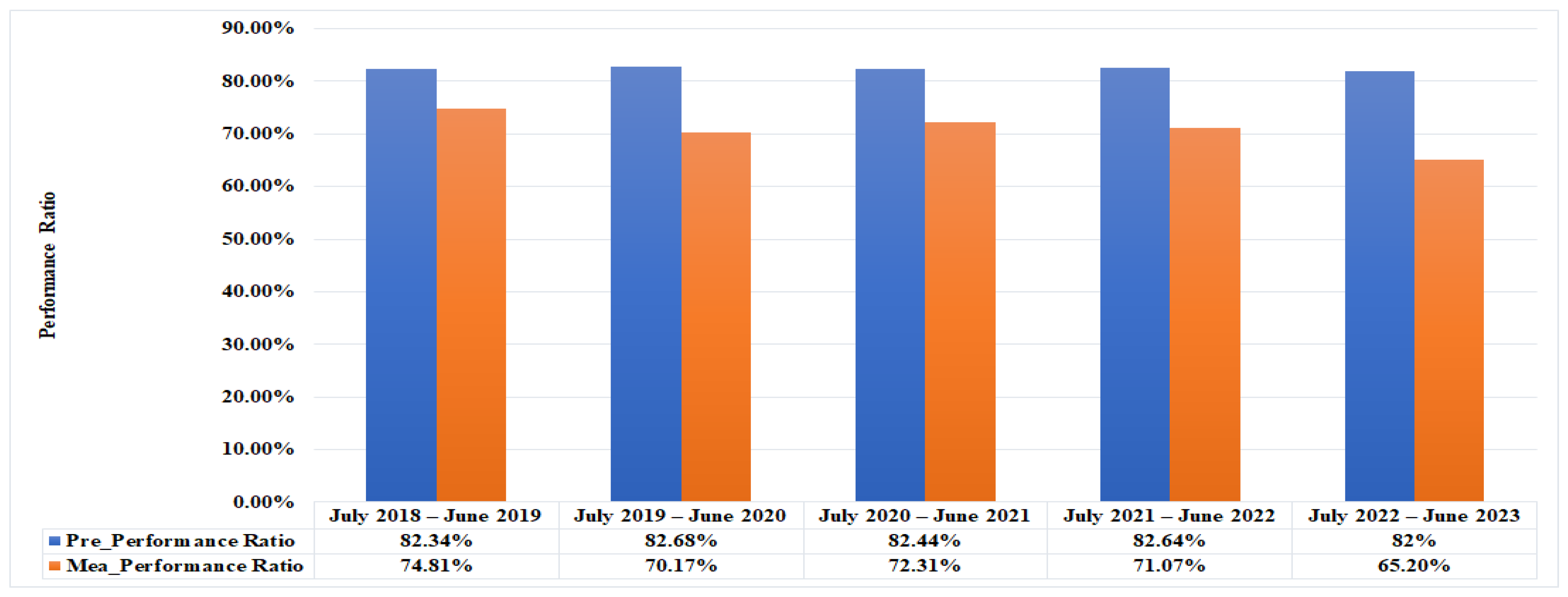
4.3. Performance Analysis

The Loss diagram for the five years (i.e., from July 2018 to June 2019, from July 2019 to June 2020, from July 2020 to June 2021, from July 2021 to June 2022, and from July 2022 to June 2023) are depicted in Figure 6, Figure 7, Figure 8, Figure 9, and Figure 10 respectively. The relationship between the measured and predicted capture loss, the system loss, and the PR is depicted in Figure 11. Figure 12 depicts the variation of PV efficiency and capacity utilization factor with regard to performance ratio. Figure 13 depicts the variation of PR and energy generation of measured and predicted values. The annual performance analysis of the system for these five years is discussed below.

For the first year, from July 2018 to June 2019, Figure 11 shows that the maximum recorded capture loss was 2.65 kWh/kW_p/day (i.e., June 19), while the lowest recorded capture loss was 0.58 kWh/kW_p/day (i.e., December 18). The highest measured system loss was 0.22 kWh/kW_p/day (November 2018), while the lowest measured system loss was 0.04 kWh/kW_p/day (i.e., June 2019). From Figure 11, it can be seen that both the predicted and measured capture loss and system values were almost similar. Figure 6 shows that a significant portion of the loss can be attributed to PV loss due to temperature, which resulted in a reduction of 9.69% from the array nominal energy. Additionally, inverter loss during operation accounted for approximately 3.00% of the energy loss from the array nominal energy, affecting the overall system efficiency. The maximum CUF value was 18.55% (April 2019), while the minimum CUF value was 7.67 (June 2019). The PR varies from 40.62% (June 2019) to 82.81% (December 2018). The maximum and minimum PV efficiency values ere 13.60 (Nov 18) and 6.50 (June 19), respectively. From Figure 12, it can be seen that when PR was high, then system efficiency was also high, and vice versa.

During the second year, from July 2019 to June 2020, the highest measured capture loss was 3.85 kWh/kW_p/day (July 2019), while the lowest measured capture loss was 0.51 kWh/kW_p/day (i.e., Jan 2020), as shown in Figure 11. The highest measured system loss was 0.38 kWh/kW_p/day (August 2019), while the lowest measured system loss was 0.01 kWh/kW_p/day (i.e., July 2019). From Figure 11 it can be seen that both the predicted and measured capture loss and system values were almost similar. Figure 7 shows that a significant portion of the loss can be attributed to PV loss due to temperature, which resulted in a reduction of 9.28% from the array nominal energy. Additionally, inverter loss during operation accounted for approximately 3.02% of the energy loss from the array nominal energy, affecting the overall system efficiency. The maximum CUF value was 16.80% (April 2020), while the minimum CUF value was 1.59% (July 2019). The PR varied from 8.98% (July 2019) to 84.43% (Jan 2020), respectively. From Figure 12 can be seen that when the PR was high, then system efficiency was also high, and vice versa.

During the third year, from July 2020 to June 2021, the highest measured capture loss was 1.68 kWh/kW_p/day (April 2021), while the lowest measured capture loss was 0.71 kWh/kW_p/day (i.e., July 2020), as shown in Figure 11. The highest measured system loss was 0.09 kWh/kW_p/day (April 2021), while the lowest measured system loss was 0.06 kWh/kW_p/day (i.e., June 2021). From Figure 11 it can be seen that both the measured and predicted capture loss and system values were almost similar. Figure 8 shows that a significant portion of the loss can be attributed to PV loss due to temperature, which resulted in a reduction of 9.65% from the array nominal energy. Additionally, inverter loss during operation accounted for approximately 2.99% of the energy loss from the array nominal energy, affecting the overall system efficiency. The maximum CUF value was 16.71% (April 2021), while the minimum CUF value was 11.58 (June 2021). The PR varied from 64.92% (June 2021) to 81.35% (Nov 2020). The maximum and minimum PV efficiency values were 13.02 (Nov 2020) and 9.66 (June 2021), respectively. From Figure 12 it can be seen that when the PR was high, then system efficiency was also high, and vice versa.

During the fourth year, from July 2021 to June 2022, the highest measured capture loss was 1.68 kWh/kW_p/day (March 2022), while the lowest measured capture loss was 0.65 kWh/kW_p/day (i.e., Dec 2021), as shown in Figure 11. The highest measured system loss was 0.09 kWh/kW_p/day (Feb 2022), while the lowest system loss was 0.06 kWh/kW_p/day (i.e., July 2021, Aug 2021, May 2022 and June 2022). From Figure 11 it can be seen that both the predicted and measured capture loss and system values were almost similar. Figure 9 shows that a significant portion of the loss can be attributed to PV loss due to temperature, which resulted in a reduction of 9.24% from the array nominal energy. Additionally, inverter loss during operation accounted for approximately 3.05% of the energy loss from the array nominal energy, affecting the overall system efficiency. The maximum CUF value was 15.98% (Feb 2022), while the minimum CUF value was 10.38% (May 2022). The PR varied from 61.48% (May 2022) to 82.06% (Nov 2021). The maximum and minimum PV efficiency values were 13.13 (Nov 2021) and 9.79 (May 2022), respectively. From Figure 12 it can be seen that when the PR was high, then system efficiency was also high, and vice versa.

During the fifth year, from July 2022 to June 2023, the highest measured capture loss was 2.83 kWh/kW_p/day (May 2023), while the lowest measured capture loss was 0.8 kWh/kW_p/day (i.e., Nov 2022), as shown in Figure 11. The highest measured system loss was 0.09 kWh/kW_p/day (Nov 2022), while the lowest measured system loss was 0.05 kWh/kW_p/day (i.e., June 2023). From Figure 11 it can be seen that both the predicted and measured capture loss and system values were almost similar. Figure 10 shows that a significant portion of the loss can be attributed to PV loss due to temperature, which resulted in a reduction of 10.13% from the array nominal energy. Additionally, inverter loss during operation accounted for approximately 2.98% of the energy loss from the array nominal energy, affecting the overall system efficiency. The maximum CUF value was 15.68% (Nov 2022), while the minimum CUF value was 9.76 (June 2023). The PR varied from 45.53% (May 2023) to 80.87% (Nov 2022). The maximum and minimum PV efficiency values were 12.94 (Nov 2022) and 7.29 (May 2023), respectively. From Figure 12 it can be seen that when the PR was high, then system efficiency was also high, and vice versa.

A summary of the performance analysis of these five years is discussed below: (a) During the period of 5 years from July 2018 to June 2023, the measured capture loss varied from Jan 2020 (i.e., 0.51 kWh/kW_p/day) to July 2019 (i.e., 3.85 kWh/kW_p/day), while the average value was 1.26 kWh/kW_p/day, as shown in Figure 11. (b) The highest measured system loss was obtained in the month of August 2019 (i.e., 0.38 kWh/kW_p/day), and the lowest measured system loss was obtained in the month of July 2019 (i.e., 0.01 kWh/kW_p/day), while the average value was 0.08 kWh/kW_p/day. Measured capture loss and system loss values were found to be almost similar to the expected values. (c) The highest CUF was obtained in April 2019 (18.44%), and the lowest CUF was obtained in July 2019 (1.59%). The average CUF was 13.36%, which is better compared to many locations, as presented in Table 5. From Figure 12 it can be seen that the measured average CUF value was 13.36%, but the lowest value was 1.59% in the month of July 2019, because during the end of the initial year, the inverter failed, i.e., on 17 June 2019, and it was resolved at the start of the second year, i.e., 27 July 2019. This was the main reason the CUF was very low in this particular month; otherwise, it should have been almost similar to other months. (d) The highest measured PR was 84.43% (i.e., January 2020), and the lowest measured PR was 8.98% (i.e., July 2019), while the measured average PR was 70.71%. (e) The highest SPV efficiency was obtained in the month of November 2018 (i.e., 13.6%), and the lowest SPV efficiency was obtained in the month of July 2019 (i.e., 1.44%), while the average value was 11.31%. Here, also due to the inverter failure during the month of July 2019, the SPV efficiency was very low compared to other months of this whole five years. Moreover, due to the inverter failure at the end of the initial year and resolved at the start of the second year, the PV efficiency of these two years was slightly low. With this information, it can be said that if the inverter had not failed to work, the PV efficiency value would have been higher than what it was for that year, and the suggested PV system would have worked better overall.

Figure 14 presents a comparison of PR across five years (i.e., from July 2018 to June 2023). The measured average PR of the last five years (i.e., 74.81% in the first year, 70.17% in the second year, 72.31% in the third year, 71.07% in the fourth year, and 65% in the fifth year) was comparable to the predicted results. The average PR of these five years was 70.71%, which was better than that of many locations, as presented in Table 5. From Figure 14 it can be seen that the PR of the system decreased gradually from the first year to the last year due to the solar panel degradation as it became older. But, in the second year, the performance ratio was lower than in the third year because, on 17 June 2019, the inverter failed due to a surge and was sent for repair to the company, which was resolved on 27 July 2019; otherwise, the performance ratio of this second year should have been higher than the third year. Furthermore, it was concluded that the performance ratio of the photovoltaic system was dependent upon the condition of the solar panels. Consequently, regular cleaning and health monitoring of the solar panels is essential. Table 5 presents a comparison of the performance of several grid-connected PV systems.

The performance of the 10 kW_p rooftop PV system was highly influenced by climatic conditions, including solar irradiance, temperature, and clearness index. Over five years (July 2018–June 2023), GHI ranged from 3.68 kW/m²/day (June 2022) to 5.78 kW/m²/day (April 2023), with higher values in pre-monsoon months boosting energy yield, while monsoon cloud cover reduced it. Temperature variations between 12.85 °C (January 2020) and 24.82 °C (June 2023) reduced efficiency since high temperatures caused thermal losses, reducing performance, especially in summer. While monsoon humidity and soiling resulted from variations in expected outputs, a clearness index, highest in winter (0.68 in January 2019), enhanced PV efficiency. System dependability could be improved by means of seasonal changes, cooling techniques, and optimal inverter settings.

The 10 kW_p rooftop PV system’s PR slowly went down over the five-year study period, from 74.81% in the first year to 65% in the fifth. This was mostly due to the degradation of the modules, the ineffectiveness of the inverter, and the climate variation. The seasonal patterns show that PR was highest in the winter (November–January) when temperatures were lower and heat losses were lower, making modules more efficient. On the other hand, PR went down during the summer and monsoon months (June–August) because of higher temperatures, more diffuse radiation, and soiling losses. The temporary PR drops were brought on by inverter failures, like the June 2019 outage, whereas the accumulation of dust and the ageing of PV modules were the main causes of the changes in PR in the long term. The measured and predicted PR showed the need for better cleaning schedules, real-time temperature correction in predictive models, and increased inverter maintenance for long-term system reliability.

This study’s observed and simulated results differed due to many real-world elements not fully accounted for in the PVsyst modelling. PVsyst uses long-term averaged meteorological records, which may not capture short-term solar radiation, temperature, and cloud cover changes. High humidity, monsoon-induced cloud cover, and seasonal changes affect electricity generation in Manipur, deviating from PVsyst forecasts. Sharma et al. (Bhubaneswar, India 11.2 kW_p) [28] found comparable cloud-induced GHI inconsistencies, resulting in lower CUF and PR values than expected. Similar to this study, Minai et al. (Lucknow, India 467.2 kW_p) [20] revealed that seasonal solar radiation changes affected performance.

Table 5 shows how climate and installation affect performance. Kumar et al. (Tiruchirappalli, India 20 kW_p) [25] and Sundaram et al. (Tamil Nadu, India 5 MWp) [30] achieved higher CUF and PR values due to consistent weather and optimal installation settings. Manipur and Ethiopia have higher humidity and cloud cover, which reduces performance (Kebede et al., 10 kW_p) [31]. Sharma et al. (Khatkar-Kalan, 190 kW_p) [12] found that decreased daylight hours affected winter performance, which affects Manipur’s energy output. New Zealand (Wellington, 10 kW_p) [34] and Ireland (13 kW_p) [32] have lower solar insolation than Manipur, resulting in lower energy production.

Installation variables also affect performance. Optimized tilt angles and tracking technologies improved energy collection efficiency year-round in Tamil Nadu (Sundaram et al., 5 MWp) [30] and Roorkee (Pundir, 1816 kW_p) [33]. In contrast, Manipur’s fixed-tilt system produced significant seasonal output changes, similar to Ethiopia (Kebede et al., 10 kW_p) [31]. In Karnataka, India (3000 kW_p) [35] and Lucknow, India (467.2 kW_p) [20], grid instabilities restricted power injection despite excellent weather. Grid stability and inverter efficiency also affect energy export potential.

Several modifications can reduce these differences and boost system performance. Instead of using historical averages, PVsyst modelling should use real-time meteorological datasets to capture short-term solar radiation and temperature fluctuations. In Tamil Nadu, India [30] and Karnataka, India [35], soiling loss models were refined to capture seasonal accumulation tendencies to improve energy yield forecasts. Improved ventilation or passive cooling could reduce temperature-induced power losses in Ethiopia [31] and Tamil Nadu, India [30]; however, there are few studies on this topic. Additionally, predictive inverter maintenance and grid stabilizing strategies, as indicated in Roorkee, India [33] and Lucknow, India [20], can improve system efficiency and eliminate simulation-to-performance disparities.

In Assam, a study by Das et al. [6] on MW-scale rooftop and ground-mounted solar power plants revealed that actual PR was less than planned, at 70.1% for rooftop and 77.8% for ground-mounted systems, owing to inverter faults, grid failures, and bad weather. These results match the variations in the PR of our system, especially in the monsoon and summer months. Likewise, the feasibility study by Kalita et al. [36] underlined how performance was much influenced by real-world elements such ambient temperature, cloud cover, and rainfall, even if simulation techniques indicated high PR values (up to 0.855 for Guwahati and Gangtok). This aligns with our observations in which measured values differed from PVsyst forecasts during highly cloudy or high-temperature seasons. Barman et al. [37] also assessed solar home lighting systems in rural Assam, noting that limited operational hours and lower system dependability resulting from technical problems and inadequate maintenance—especially during monsoons. These investigations confirm our conclusion that to increase the accuracy of simulations, models must include real-time environmental conditions, maintenance problems, and system-specific losses. By comparing with these regional findings, our study better contextualizes the observed performance gaps and emphasizes the importance of site-specific adjustments in solar PV performance forecasting.

4.4. Actual Economic Analysis

Under the electricity regulatory commission, the government of Manipur had approved on 2 November 2016 that the total cost of each kW_p is Rs 60,000/- for (1–10 kW) rooftop solar power system.

• Capital Cost = Rs 600,000/-.
• Subsidy (70% of the capital cost) = Rs 420,000/-.
• Actual cost = Capital Cost − Subsidy = Rs 180,000/-.
• Selling price per unit kWh = Rs 3.16/-.
• From Figure 13, it can be seen that at the end of 4 years and 10 months, the generation of energy reaches 57,449.2 kWh.
• Recovery amount at the end of 4 years and 10 months = Eg × Selling price per unit kWh = 57,449.2 × 3.16 =Rs 181,539.47/-

It was found that the actual simple payback was 4 years and 10 months to recover the actual cost of the suggested PV system after receiving a 70% subsidy. The proposed project’s life span was 25 years, and its invested cost was recovered within 4 years and 10 months. Therefore, the suggested solar photovoltaic system demonstrates superior energy output and performance relative to other systems placed in different locations, as illustrated in Table 5. Moreover, the total amount of energy sold to the grid during these 5 years (i.e., July 2018 to June 2023) was 58,911.3 kWh.

It was found that PV systems have higher initial installation costs than conventional energy sources like coal, natural gas, oil, etc. However, their operational costs over time are lower due to little maintenance and no fuel expenses, making them more cost-effective. In addition to the financial and environmental advantages in the long run, PV systems help the environment by cutting down on the emission of greenhouse gases.

5. Conclusions

The technical parameters of the 10 kW_p rooftop grid-connected PV system from July 2018 to June 2023 were evaluated and also compared with the simulated result. The results of the research are presented below:

The system generated, on average, 32.26 kWh/day over five years; its specific energy yield was 3.20 kWh/kW_p. The highest measured energy generation months were quite similar to the simulated result for the first four years. In addition, it revealed that the energy generation was less during the rainy season (i.e., June, July, August, and September) and winter season (i.e., December, January, and February). This highlights the need for seasonally adjusted energy management strategies, such as incorporating storage solutions or grid integration techniques to maintain supply reliability during low-generation periods.

The daily measured PR of the system for 5 years was 70.71% (which was almost 86.23% of the predicted value), even including the 40 days OFF due to inverter failure. The measured Lc was less in the winter season (i.e., Nov, Dec, and Jan), which was almost similar to the simulated results except for a slight difference in the initial year. Regular system health checks and fault detection mechanisms could further reduce downtime and improve PR stability over the years.

The loss diagram analysis over a five-year period revealed that inverter losses contributed to approximately 3% of the total energy loss, while capture losses due to temperature effects accounted for approximately 9.69%. Particularly during the months of high irradiance (April–July), when module temperatures increase, these losses had an effect on the overall efficacy of the system. To reduce these losses, it is recommended that cooling strategies be implemented, inverter operation be optimized, and energy conversion be ensured to be efficient.

The PV system efficiency and capacity factor were found to be 13.36% and 11.31%, respectively, which were nearly comparable to other systems placed in various locations across the globe. However, performance can be further optimized by implementing periodic panel cleaning to mitigate soiling losses and ensuring optimal inverter operation to minimize conversion losses.

The investigation found that the actual payback period was 4 years and 10 months. The measured and predicted energy generation for the whole five years was 58,911.3 kWh and 77,769 kWh, respectively. It was revealed that the measured value was almost 75.75% of the predicted value, indicating a strong return on investment. Improved net-metering regulations and increased government incentives could help future installations in Manipur and comparable areas to promote broader use of grid-connected PV systems.

References

1. Li, C. Economic and performance evaluation of grid-connected residential solar photovoltaic systems in Northwest China. Energy Sources Part A Recovery Util. Environ. Eff. 2022, 44, 5473–5489. [Google Scholar] [CrossRef]
2. Teyabeen, A.A.; Algareu, A.; Mohamed, F. Assessment of Solar Photovoltaic System Performance. In Proceedings of the 2023 14th International Renewable Energy Congress (IREC), IEEE, Sousse, Tunisia, 16–18 December 2023; pp. 1–5. [Google Scholar]
3. Liu, J. China's renewable energy law and policy: A critical review. Renew. Sustain. Energy Rev. 2019, 99, 212–219. [Google Scholar] [CrossRef]
4. Kamble, A.D.; Das, S.; Vijaya; Das, B.; Bordoloi, U.; Hazarika, P.; Kalita, P. Role of Solar Energy in the Development of the Indian Economy. In Challenges and Opportunities of Distributed Renewable Power; Springer Nature: Singapore, 2024; pp. 489–535. [Google Scholar]
5. Dhiman, B.; Zindani, D.; Chakrabarti, D.; Singh, G. A user-centric assessment of solar-photovoltaic-home-lighting systems in rural parts of Assam, India. Energy Sustain. Dev. 2023, 76, 101290. [Google Scholar] [CrossRef]
6. Das, D.; Saikia, S.; Saharia, S.J.; Mahapatra, S. Performance analysis of MW-scale grid connected rooftop and ground-mounted solar power plants installed in Assam, India. Energy Sustain. Dev. 2023, 76, 101309. [Google Scholar] [CrossRef]
7. Tajjour, S.; Chandel, S.S.; Chandel, R.; Thakur, N. Power generation enhancement analysis of a 400 kWp grid-connected rooftop photovoltaic power plant in the hilly terrain of India. Energy Sustain. Dev. 2023, 77, 101333. [Google Scholar] [CrossRef]
8. Aktas, I.S.; Ozenc, S. A case study of techno-economic and environmental analysis of college rooftop for grid-connected PV power generation: Net zero 2050 pathway. Case Stud. Therm. Eng. 2024, 56, 10427. [Google Scholar] [CrossRef]
9. Mohamed, K.; Shareef, H.; Nizam, I.; Esan, A.B.; Shareef, A. Operational Performance Assessment of Rooftop PV Systems in the Maldives. Energy Rep. 2024, 11, 2592–2607. [Google Scholar] [CrossRef]
10. Attari, K.; Elyaakoubi, A.; Asselman, A. Performance analysis and investigation of a grid-connected photovoltaic installation in Morocco. Energy Rep. 2016, 2, 261–266. [Google Scholar] [CrossRef]
11. de Lima, L.C.; de Araújo Ferreira, L.; de Lima Morais, F.H. Performance analysis of a grid-connected photovoltaic system in northeastern Brazil. Energy Sustain. Dev. 2017, 37, 79–85. [Google Scholar] [CrossRef]
12. Sharma, V.; Chandel, S.S. Performance analysis of a 190 kWp grid interactive solar photovoltaic power plant in India. Energy 2013, 55, 476–485. [Google Scholar] [CrossRef]
13. Aryal, A.; Bhattarai, N. Modeling and simulation of 115.2 kWp grid-connected solar PV system using PVSYST. Kathford J. Eng. Manag. 2018, 1, 31–34. [Google Scholar] [CrossRef]
14. Arora, R.; Arora, R.; Sridhara, S.N. Performance assessment of 186 kWp grid interactive solar photovoltaic plant in Northern India. Int. J. Ambient Energy 2022, 43, 128–141. [Google Scholar] [CrossRef]
15. Ramanan, P.; Karthick, A. Performance analysis and energy metrics of grid-connected photovoltaic systems. Energy Sustain. Dev. 2019, 52, 104–115. [Google Scholar]
16. Ramanan, P.; Kalidasa Murugavel, K.; Karthick, A.; Sudhakar, K. Performance evaluation of building-integrated photovoltaic systems for residential buildings in southern India. Build. Serv. Eng. Res. Technol. 2020, 41, 492–506. [Google Scholar] [CrossRef]
17. Kumar, M.; Chandel, S.S.; Kumar, A. Performance analysis of a 10 MWp utility scale grid-connected canal-top photovoltaic power plant under Indian climatic conditions. Energy 2020, 204, 117903. [Google Scholar] [CrossRef]
18. Dahbi, H.; Aoun, N.; Sellam, M. Performance analysis and investigation of a 6 MW grid-connected ground-based PV plant installed in hot desert climate conditions. Int. J. Energy Environ. Eng. 2021, 12, 577–587. [Google Scholar] [CrossRef]
19. Navothna, B.; Thotakura, S. Analysis on large-scale solar PV plant energy performance–loss–degradation in coastal climates of India. Front. Energy Res. 2022, 10, 857948. [Google Scholar] [CrossRef]
20. Minai, A.F.; Usmani, T.; Alotaibi, M.A.; Malik, H.; Nassar, M.E. Performance analysis and comparative study of a 467.2 kWp grid-interactive SPV system: A case study. Energies 2022, 15, 1107. [Google Scholar] [CrossRef]
21. Besheer, A.H.; Eldreny, M.A.; Rashad, H.; Bahgat, A. Status monitoring and performance investigation of a 5.1 kW rooftop grid-tie photovoltaic energy system. In Modern Maximum Power Point Tracking Techniques for Photovoltaic Energy Systems; Springer: Cham, Switzerland, 2019; pp. 463–486. [Google Scholar]
22. Sharma, V.; Kumar, A.; Sastry, O.S.; Chandel, S.S. Performance assessment of different solar photovoltaic technologies under similar outdoor conditions. Energy 2013, 58, 511–518. [Google Scholar] [CrossRef]
23. Ayompe, L.M.; Duffy, A.; McCormack, S.J.; Conlon, M. Measured performance of a 1.72 kW rooftop grid-connected photovoltaic system in Ireland. Energy Convers. Manag. 2011, 52, 816–825. [Google Scholar] [CrossRef]
24. Okello, D.; Van Dyk, E.E.; Vorster, F.J. Analysis of measured and simulated performance data of a 3.2 kWp grid-connected PV system in Port Elizabeth, South Africa. Energy Convers. Manag. 2015, 100, 10–15. [Google Scholar] [CrossRef]
25. Kumar, K.A.; Sundareswaran, K.; Venkateswaran, P.R. Performance study on a grid connected 20 kWp solar photovoltaic installation in an industry in Tiruchirappalli (India). Energy Sustain. Dev. 2014, 23, 294–304. [Google Scholar] [CrossRef]
26. Yadav, S.K.; Bajpai, U. Performance evaluation of a rooftop solar photovoltaic power plant in Northern India. Energy Sustain. Dev. 2018, 43, 130–138. [Google Scholar] [CrossRef]
27. Vasisht, M.S.; Srinivasan, J.; Ramasesha, S.K. Performance of solar photovoltaic installations: Effect of seasonal variations. Sol. Energy 2016, 131, 39–46. [Google Scholar] [CrossRef]
28. Sharma, R.; Goel, S. Performance analysis of a 11.2 kWp roof top grid-connected PV system in Eastern India. Energy Rep. 2017, 3, 76–84. [Google Scholar] [CrossRef]
29. Vasudev, K.P.; Mathew, M.; Anand, A.; Hossain, J. Performance Analysis of a 48 kWp Grid connected Rooftop Photovoltaic System. In Proceedings of the 2018 4th International Conference for Convergence in Technology (I2CT), IEEE, Mangalore, India, 27–28 October 2018; pp. 1–6. [Google Scholar]
30. Sundaram, S.; Babu, J.S. Performance evaluation and validation of 5 MWp grid connected solar photovoltaic plant in South India. Energy Convers. Manag. 2015, 100, 429–439. [Google Scholar] [CrossRef]
31. Kebede, A.A.; Berecibar, M.; Coosemans, T.; Messagie, M.; Jemal, T.; Behabtu, H.A.; Van Mierlo, J. A techno-economic optimization and performance assessment of a 10 kWP photovoltaic grid-connected system. Sustainability 2020, 12, 7648. [Google Scholar] [CrossRef]
32. Mondol, J.D.; Yohanis, Y.; Smyth, M.; Norton, B. Long term performance analysis of a grid connected photovoltaic system in Northern Ireland. Energy Convers. Manag. 2006, 47, 2925–2947. [Google Scholar] [CrossRef]
33. Pundir, K.S.; Varshney, N.; Singh, G.K. Comparative study of performance of grid connected solar photovoltaic power system in IIT Roorkee campus. Int. J. Innov. Res. Sci. Eng. 2016, 2, 319–422. [Google Scholar]
34. Emmanuel, M.; Akinyele, D.; Rayudu, R. Techno-economic analysis of a 10ákWp utility interactive photovoltaic system at Maungaraki school, Wellington, New Zealand. Energy 2017, 120, 573–583. [Google Scholar] [CrossRef]
35. Padmavathi, K.; Daniel, S.A. Performance analysis of a 3 MWp grid connected solar photovoltaic power plant in India. Energy Sustain. Dev. 2013, 17, 615–625. [Google Scholar] [CrossRef]
36. Kalita, P.; Das, S.; Das, D.; Borgohain, P.; Dewan, A.; Banik, R.K. Feasibility study of installation of MW level grid connected solar photovoltaic power plant for northeastern region of India. Sādhanā 2019, 44, 207. [Google Scholar] [CrossRef]
37. Barman, M.; Mahapatra, S.; Palit, D.; Chaudhury, M.K. Performance and impact evaluation of solar home lighting systems on the rural livelihood in Assam, India. Energy Sustain. Dev. 2017, 38, 10–20. [Google Scholar] [CrossRef]
Figure 1. Proposed diagram of the 10 kWp rooftop grid-connected PV system.
Energies 18 01921 g001
Figure 2. Google map image of the proposed PV system.
Energies 18 01921 g002
Figure 3. Variation of daily monthly GHI, DHI, Amb_temp, and clearness index.
Energies 18 01921 g003
Figure 4. The monthly energy yield of predicted and measured with regard to the DHI and GHI.
Energies 18 01921 g004
Figure 5. Daily Monthly variations in measured and predicted array yield and final yield are compared to the reference yield and temperature.
Energies 18 01921 g005
Figure 6. Loss diagram for the first year (i.e., from July 2018 to June 2019).
Energies 18 01921 g006
Figure 7. Loss diagram for the second year (i.e., from July 2019 to June 2020).
Energies 18 01921 g007
Figure 8. Loss diagram for the third year (i.e., from July 2020 to June 2021).
Energies 18 01921 g008
Figure 9. Loss diagram for the fourth year (i.e., from July 2021 to June 2022).
Energies 18 01921 g009
Figure 10. Loss diagram for the fifth year (i.e., from July 2022 to June 2023).
Energies 18 01921 g010
Figure 11. Variation in measured and predicted capture loss and system loss with regard to performance ratio.
Energies 18 01921 g011
Figure 12. Variation of PV efficiency and capacity utilization factor with regard to performance ratio.
Energies 18 01921 g012
Figure 13. Variation of PR and energy generation of measured and predicted values.
Energies 18 01921 g013
Figure 14. Comparison of PR in five years (i.e., from July 2018 to June 2023).
Energies 18 01921 g014