Applicability Analysis of Reduced-Order Methods with Proper Orthogonal Decomposition for Neutron Diffusion in Molten Salt Reactor

Abstract

The high-dimensional integral–differential nature of the neutron transport equation and the complexity of nuclear reactors result in high computational costs. A set of reduced-order modeling frameworks based on Proper Orthogonal Decomposition (POD) is developed to improve the computational efficiency for neutron diffusion calculations while maintaining accuracy, especially for small samples. For modal coefficient calculations, three methods—Galerkin, radial basis function (RBF), and Deep Neural Network (DNN)—are introduced and analyzed for molten salt reactors. The results show that all three reduced-order models achieve sufficient accuracy, with neutron flux L₂ errors below 1% and delayed neutron precursor (DNP) L₂ errors below 2.4%, while the acceleration ratios exceed 800. Among these, the POD–Galerkin model demonstrates superior performance, achieving average L₂ errors of less than 0.00658% for neutron flux and 1.01% for DNP concentration, with an acceleration ratio of approximately 1800 and excellent extrapolation ability. The POD–Galerkin reduced-order model significantly enhances the computational efficiency for solving neutron multi-group diffusion equations and DNP conservation equations in molten salt reactors while preserving the solution accuracy, making it ideal for a liquid fuel molten salt reactor in the case of small samples.

1. Introduction

Physical calculations for reactors play an important role in nuclear reactor design, safe operation monitoring, and reactor accident prediction. With the improvement in core modeling and simulation accuracy, the computational complexity is increasing, and improving the computational efficiency is one of the main research directions in the development of reactor physical computing. For neutron transport calculations in molten salt reactors, models such as classical finite element methods [1,2], finite volume methods, and other numerical methods using high-resolution grids [3,4] typically employ numerical schemes that cast the problem onto a discretized domain, which leads to high-dimensional parameters and response spaces. Even with the parallel computing power of supercomputers, there are still efficiency challenges when facing problems that require multiple, fast, or even real-time solutions [5]. To fulfill practical requirements, it is imperative to significantly enhance the computational efficiency of reactor physics analyses [6]. Consequently, simplified (or surrogate) models that are computationally efficient and reasonably accurate are often sought to carry out such calculations.

The reduced-order model (ROM) is an efficient technique for reducing the resources required for calculation. It proposes characteristics from existing physical snapshots and efficiently predicts unknown physical processes based on these characteristics. Compared to the full-order model, the ROM enhances the computational efficiency while incurring a certain degree of accuracy loss. Common model order reduction methods include Proper Orthogonal Decomposition, Chebyshev polynomial reduction, Laguerre–Singular Value Decomposition, etc. POD is a powerful dimensionality reduction technique that extracts dominant coherent structures from high-dimensional datasets, enabling efficient representation of complex dynamical systems [7]. The POD method can effectively extract the principal components of the physical process, and Holmes et al. [8] proved that the POD method is the best approximation of the original system in steady-state calculations. Reduced-order models based on POD are typically constructed by intrusive or non-intrusive methods [9]. Intrusive methods include a variety of projection techniques that directly access the underlying model and generally have good interpretability. The non-intrusive approach is data-driven, runs simulations in a black box mode, and learns mapping functions through regression, interpolation, or other machine learning techniques [10,11].

In recent years, the ROM has been widely applied in nuclear reactor engineering to enhance computational efficiency [12]. Buchan et al. [13] used a reduced-order model based on the POD method to quickly solve 1D and 2D neutron diffusion eigenvalue problems. Among the intrusive methods, the POD method is more widely used. Sartori et al. [14] compared the Modal Method (MM) with the POD method for multi-group neutron diffusion dynamics and analyzed the ability of the POD method to evaluate the reactivity and neutron flux of different reactor configurations. German and Ragusa [15] used the POD-based ROM to parameterize the multi-group neutron diffusion k-eigenvalue problem and obtained a remarkable speed-up factor. Furthermore, Prince and Ragusa [16] used the PGD approach to analyze the uncertainty quantification of the neutron diffusion equation with external sources.

Non-intrusive model reduction methods enable efficient system approximation by leveraging input–output data without modifying the original high-fidelity solver, making them ideal for complex black box simulations or experimental datasets. POD-RBF, a hybrid approach combining Proper Orthogonal Decomposition for mode extraction and radial basis function interpolation for parametric surrogate modeling, effectively combines dimensionality reduction with adaptive response prediction across varying operating conditions. The RBF neural network has the advantages of a strong nonlinear mapping ability, insensitivity to the input dimension, and a simple grid structure, and when dealing with nonlinear problems, it has the advantage of high stability [17]. Arka Das et al. [18] proposed a numerical reduced-order model framework combining the POD method and the radial basis function to provide quantitative and qualitative analyses of thermomechanical responses. With the rapid development of neural network technology, the POD method is gradually being combined with neural network technology to avoid the calculation of numerical equations [19,20,21]. Mattia Massone et al. [22] proposed an algorithm based on the genetic algorithm that can select energy group boundaries for different reactor systems to collapse a fine multi-group library into one with a few groups and verified it in three reactor systems: ESNII + ASTRID, ESFR, and MSFR. Wei et al. [23] proved that POD-DNN is a general-purpose neural network solution that is capable of learning complex patterns in data, suitable for training unstructured data.

As one of the fourth-generation candidate advanced nuclear reactor systems, the molten salt reactor (MSR) is capable of operating safely under high-temperature conditions and at low pressure [24]. It also enables online fueling and breeding, thereby minimizing the generation of nuclear waste. Moreover, the high boiling point and excellent thermal conductivity of molten salts in liquid fuel MSRs contribute to an inherently safe reactor core. However, the flow characteristics of liquid fuels present a significant challenge for neutron physics calculations. The movement of molten salt can alter the distribution of delayed neutron precursor nuclei, leading to unique dynamic behaviors that distinguish the neutron physical characteristics of liquid fuel MSRs from those of traditional solid fuel reactors. Consequently, these flow characteristics must be carefully considered in neutron physics calculations. According to an extensive preliminary investigation, the current theories of a reduced-order model which is suitable for neutron calculations for molten salt reactors and takes into account the delayed neutron precursors are not fully refined [25,26,27]. The DNP concentration, a pivotal parameter in neutron kinetics, is directly governed by the liquid fuel flow dynamics within molten salt reactors, as advection effects the dominate precursor transport. Consequently, the predictive fidelity of DNP concentration calculations becomes a critical metric for validating reduced-order models (ROMs) of reactor physics. To accurately and efficiently solve the neutron transport equation and the DNP conservation equation for a molten salt reactor, three reduced-order models, POD–Galerkin, POD-RBF, and POD-DNN, are constructed by intrusive and non-intrusive methods, respectively, and a modal analysis of the neutron flux and DNP concentration in molten salt reactors is conducted using the POD methodology under small-sample conditions. A systematic comparative analysis of the neutron flux and DNP concentration errors across methodologies is conducted by sampling parameters within the ranges of ±20% using Latin hypercube sampling, with the applicability of the POD-based reduced-order modeling framework being quantitatively assessed through numerical validation. The extrapolation ability of three reduced-order models is tested by using test samples that are out of the range of the training set parameters.

2. Methods

2.1. Full-Order Models

The deduction of reduced-order models for the neutron physics processes starts from the full-order models, including the neutron diffusion equations and the delayed neutron precursor balance equation under a steady state, which can be written as follows:

$$-\stackrel{\rightharpoonup }{\nabla }\cdot (D_g\stackrel{\rightharpoonup }{\nabla }{\varphi }_g)+{\sum }_{r,g}{\varphi }_g={\displaystyle \frac{{\chi }_g(1-\beta )}{k_{\mathrm{eff}}}}{\displaystyle \sum _{g^{\prime }=1}^G\nu }{\sum }_{f,g^{\prime }}{\varphi }_{g^{\prime }}+{\displaystyle \sum _{g^{\prime }\ne g}^G{\sum }_{s,g^{\prime }\to g}}{\varphi }_{g^{\prime }}+{\displaystyle \sum _{j=1}^M{\chi }_{d,j}{\lambda }_j{C}_j},\hspace{1em}\mathrm{g}\in \left[1,G\right]$$

(1)

$$\stackrel{\rightharpoonup }{\nabla }\cdot (u{C}_j)={\displaystyle \frac{1}{k_{\mathrm{eff}}}}{\displaystyle \sum _{g^{\prime }=1}^G{\beta }_j\nu }{\sum }_{f,g^{\prime }}{\varphi }_{g^{\prime }}-{\lambda }_j{C}_j,\hspace{1em}j\in \left[1,P\right]$$

(2)

where ${\sum }_{r,g}$ is the removal cross-section for group g, defined as follows:

$${\sum }_{r,g}={\sum }_{a,g}+{\displaystyle \sum _{g^{\prime }\ne g}^G{\sum }_{s,g\to g^{\prime }}}$$

(3)

where ${\varphi }_g$, $D_g$, ${\sum }_{a,g}$, and $\nu {\sum }_{f,g^{\prime }}$ are the neutron flux, diffusion coefficient, absorption cross-section, and production cross-section. ${\sum }_{s,g^{\prime }\to g}$ is the scattering cross-section from group $g^{\prime }$ to group $g$, and ${\chi }_g$ is the probability that a fission neutron will be born in group g. $C_j$ is the DNP concentration, ${\beta }_j$ is the fraction of delayed neutrons, and ${\lambda }_j$ is the decay constant for group j.

The inlet boundary condition, the outlet boundary condition, and the outer wall boundary for the neutron flux are set to a zero-boundary condition. The inner wall boundary condition of the neutron flux is set as a coupling boundary condition, as shown in Equation (4):

$${\varphi }_g^A={\varphi }_g^B$$

(4)

where A and B represent two different media.

The inlet boundary condition for the DNP concentration is shown in Equation (5):

$$C_{j,inlet}=C_{j,outlet}{e}^{-{\lambda }_j{\tau }_{loop}}$$

(5)

where ${\tau }_{loop}$ is the flow time of the DNPs in the outer loop of the reactor core. The outlet boundary condition for the DNP concentration is set to a zero-gradient boundary condition. The inner wall boundary condition for the DNP concentration is set to a zero-boundary condition.

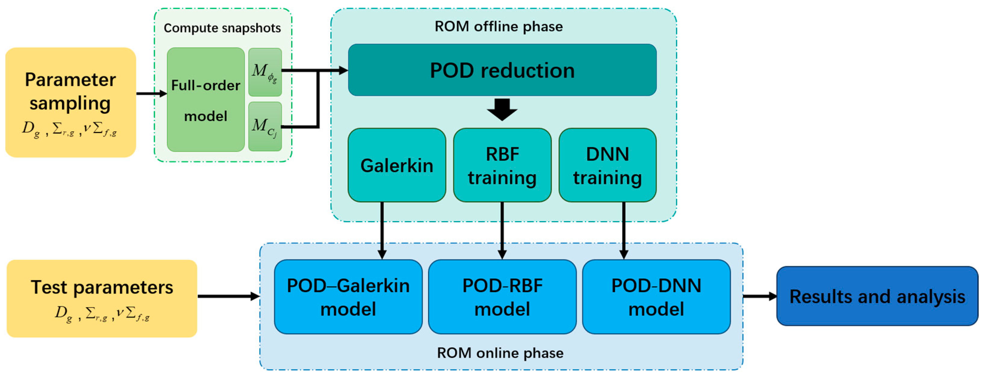
2.2. Reduced-Order Model Approaches

As shown in Figure 1, the overall calculation process for the reduced-order model for a molten salt reactor is divided into two parts, which are the offline stage and online stage. In the offline phase, the first step is to generate the snapshot set, followed by performing POD on this set. Subsequently, three reduced-order models—the POD–Galerkin model, the POD-RBF model, and the POD-DNN model—are constructed. In the online phase, these models are employed to calculate the POD modal coefficients according to the current input parameters, thereby obtaining the reduced-order results.

2.2.1. The POD–Galerkin Method

The POD method constructs an autocorrelation matrix of a certain dataset and obtains a set of ordered orthogonal basis vectors from it. It uses the first k basis vectors to approximate the original dataset; that is, it uses low-dimensional data to represent the changing characteristics of high-dimensional datasets. The snapshot method [28] is commonly used for generating offline training datasets. In this work, snapshots are generated by calculating the neutron fluxes ${\varphi }_g$ and precursor concentrations $C_j$ from different cross-sectional data under steady-state conditions. For the whole computational domain, the snapshots matrix can be represented as follows:

$${\mathrm{M}}_{{\varphi }_g}=\left\{{\varphi }_1^g,{\varphi }_2^g,{\varphi }_3^g,\cdots ,{\varphi }_m^g\right\}$$

(6)

$${\mathrm{M}}_{C_j}=\left\{C_1^j{,\mathrm{C}}_2^j,C_3^j,\cdots ,C_m^j\right\}$$

(7)

where m is the number of snapshots, $M_{{\varphi }_g}$ is the set of flux distribution snapshots, and $M_{C_j}$ is the set of precursor concentration snapshots corresponding to different cross-sections.

An optimal basis can be obtained by calculating the Singular Value Decomposition (SVD) of $M$. Meanwhile, we can define the m-order square matrix S as follows:

$$M=U\mathsf{\Sigma }{V}^T$$

(8)

$$S=M^{T}M$$

(9)

where $U$ and $V$ are the left and right singular matrices, representing the eigenvectors of $S^T$ and $S$, respectively, while $\sum$ is a diagonal matrix of singular values. Defining $\lambda =\left\{\begin{array}{cccc}{\lambda }_1& {\lambda }_2& \dots & {\lambda }_N\end{array}\right\}$ as the set of all non-zero eigenvalues of the square matrix $S$ arranged in a descending order, the POD basis can be expressed as follows:

$${\phi }_n={\displaystyle \frac{1}{\sqrt{{\lambda }_n}}}M{V}_n^T, n=1,2,\dots N$$

(10)

According to the POD theory, the magnitude of the eigenvalue represents the importance of the corresponding feature vector [29]. Therefore, the POD order k can be determined as follows:

$$k=\arg \min \left\{I\left(k\right):I\left(k\right)\ge 99.999999\%\right\},I\left(k\right)={\displaystyle \frac{{\displaystyle \sum _{i=1}^k{\lambda }_i}}{{\displaystyle \sum _{j=1}^N{\lambda }_j}}}$$

(11)

where $I\left(k\right)$ is the energy fraction of the first k-order POD modes. The POD basis constructed with k dominant POD modes is the most important part for building the reduced-order model.

Using k-order POD modes to approximate ${\varphi }_g$ and $C_j$, we can write this in a matrix form as follows:

$${\varphi }_g^R={\displaystyle \sum _{i=1}^{k_{{\varphi }_g}}{a}_i^{{\varphi }_g}{\phi }_i^{{\varphi }_g}}={\Phi }_{{\varphi }_g}{A}_{{\varphi }_g}$$

(12)

$$C_j^R={\displaystyle \sum _{i=1}^{k_{C_j}}{a}_i^{C_j}{\phi }_i^{C_j}}={\Phi }_{C_j}{A}_{C_j}$$

(13)

where $a$ is the coefficient matrix of the POD basis. Substituting the reduced form into Equations (1) and (2), and according to Galerkin projection, we can multiply ${\Phi }_{{\varphi }_g}^T$ and ${\Phi }_{C_j}^T$ to the left, respectively. Equations (1) and (2) can be written as follows:

$${\displaystyle \sum _{l=1}^{k_{{\varphi }_g}}\left\{\begin{array}{l}{\displaystyle \sum _{i=1}^{k_{{\varphi }_g}}\left(-\stackrel{\rightharpoonup }{\nabla }\cdot (D_g\stackrel{\rightharpoonup }{\nabla })+{\sum }_{r,g}\right)a_i^{{\varphi }_g}{\phi }_i^{{\varphi }_g}}-\frac{1}{k_{\mathrm{eff}}}{\chi }_g(1-\beta ){\displaystyle \sum _{g^{\prime }=1}^G\nu {\sum }_{f,g^{\prime }}{\displaystyle \sum _{i=1}^{k_{{\varphi }_{g^{\prime }}}}{a}_i^{{\varphi }_{g^{\prime }}}{\phi }_i^{{\varphi }_{g\prime }}}}\\ +{\displaystyle \sum _{g^{\prime }\ne g}^G{\sum }_{s,g^{\prime }\to g}{\displaystyle \sum _{i=1}^{k_{{\varphi }_{g^{\prime }}}}{a}_i^{{\varphi }_{g^{\prime }}}{\phi }_i^{{\varphi }_{g\prime }}}}+{\chi }_{d,g}{\displaystyle \sum _{j=1}^M{\lambda }_j{\displaystyle \sum _{i=1}^{k_{C_j}}{a}_i^{C_j}{\phi }_i^{C_j}}}\end{array}\right\}}{\phi }_l^{{\varphi }_g}=0, \mathrm{g}\in \left[1,G\right]$$

(14)

$${\displaystyle \sum _{l=1}^{k_{C_j}}\left\{{\displaystyle \sum _{i=1}^{k_{C_j}}\left(\stackrel{\rightharpoonup }{\nabla }\cdot u+{\lambda }_j\right)a_i^{C_j}{\phi }_i^{C_j}}-\frac{1}{k_{\mathrm{eff}}}{\displaystyle \sum _{g^{\prime }=1}^G{\beta }_j\nu }{\sum }_{f,g^{\prime }}{\displaystyle \sum _{i=1}^{k_{{\varphi }_{g^{\prime }}}}{a}_i^{{\varphi }_{g^{\prime }}}{\phi }_i^{{\varphi }_{g\prime }}}\right\}}{\phi }_l^{C_j}=0, j\in \left[1,P\right]$$

(15)

Therefore, the equations’ coefficient matrix order can be reduced from ${ℝ}^{s\times s}$ to ${ℝ}^{k\times k}$, where s is the original system’s mesh number, while $k\ll s$. This operation greatly reduces the solution complexity of the system, and Equations (12) and (13) can be used to rebuild the full-order system fast.

2.2.2. The POD-RBF Method

The RBF is a common multivariate interpolation function, and its general form can be written as follows:

$$x\left(p\right)={\displaystyle \sum _{i=1}^n{w}_{i}f\left(r^i\right)}$$

(16)

where x is the POD mode coefficients of the neutron flux or precursor concentration corresponding to the parameter p, $w_i$ is the weight coefficient, $r^i=\left|p-p^i\right|$ is the Euclidean distance between $p$ and $p^i$, $p$ corresponds to a vector containing arbitrary values of the design parameters, $p^i$ corresponds to the set of parameter values that are used to generate the snapshot set $M_{{\varphi }_g}$ and $M_{C_j}$, and $f\left(·\right)$ is the radial basis function. Commonly used radial basis functions include the following:

The thin-plate-spline function:

$$f\left(r\right)=r^2\ln r$$

(17)

The inverse multiquadric function:

$$f\left(r\right)={\left(r^2+c^2\right)}^{-1/2}$$

(18)

The Gaussian function:

$$f\left(r\right)=\exp \left(-r^2/c^2\right)$$

(19)

where $c>0$ denotes the RBF shape factor, which controls the steepness of the function. In this work, the radial basis function chooses the inverse multiquadric function.

Substitute all samples and default parameters into Equation (16):

$$\left[\begin{array}{c}{x}^1\\ x^2\\ ⋮\\ x^m\end{array}\right]=\left[\begin{array}{cccc}{f}_{11}& f_{12}& \dots & f_{1m}\\ f_{21}& f_{22}& \dots & f_{2m}\\ ⋮& ⋮& \ddots & ⋮\\ f_{m1}& f_{m2}& \dots & f_{mm}\end{array}\right]\cdot \left[\begin{array}{c}{w}_1\\ w_2\\ ⋮\\ w_m\end{array}\right]$$

(20)

where $f_{ij}=f\left(\left|p^i-p^j\right|\right)$ for $i,j=1,2,\dots ,m$, which can be denoted as $F$. According to the RBF interpolation method, the coefficient $a\left(p\right)$ in Equations (12) and (13) is interpolated as follows:

$$a\left(p\right)=Wf\left(r\right)$$

(21)

Since the snapshot set M has no duplicate samples, F is an invertible square matrix. For the set M, substituting Equation (21) into Equations (12) and (13) and multiplying both sides by ${\Phi }^T$ on the left and $F^{-1}$ on the right, the weight coefficient matrix W is obtained as follows:

$$W={\Phi }^{T}M{F}^{-1}$$

(22)

The POD-RBF reduced model is written as follows:

$$\Psi =\Phi \cdot \left({\Phi }^{T}M{F}^{-1}\right)\cdot f\left(r\right)$$

(23)

where $\Psi$ represents ${\varphi }_g^R$ or $C_j^R$. This model is capable of reproducing fields that correspond to an arbitrary set of parameters p, hereafter referred to as the trained RBF-POD network. Obviously, parameters which extrapolate outside the range of p that was used to generate snapshots can lead to poor accuracy of the model.

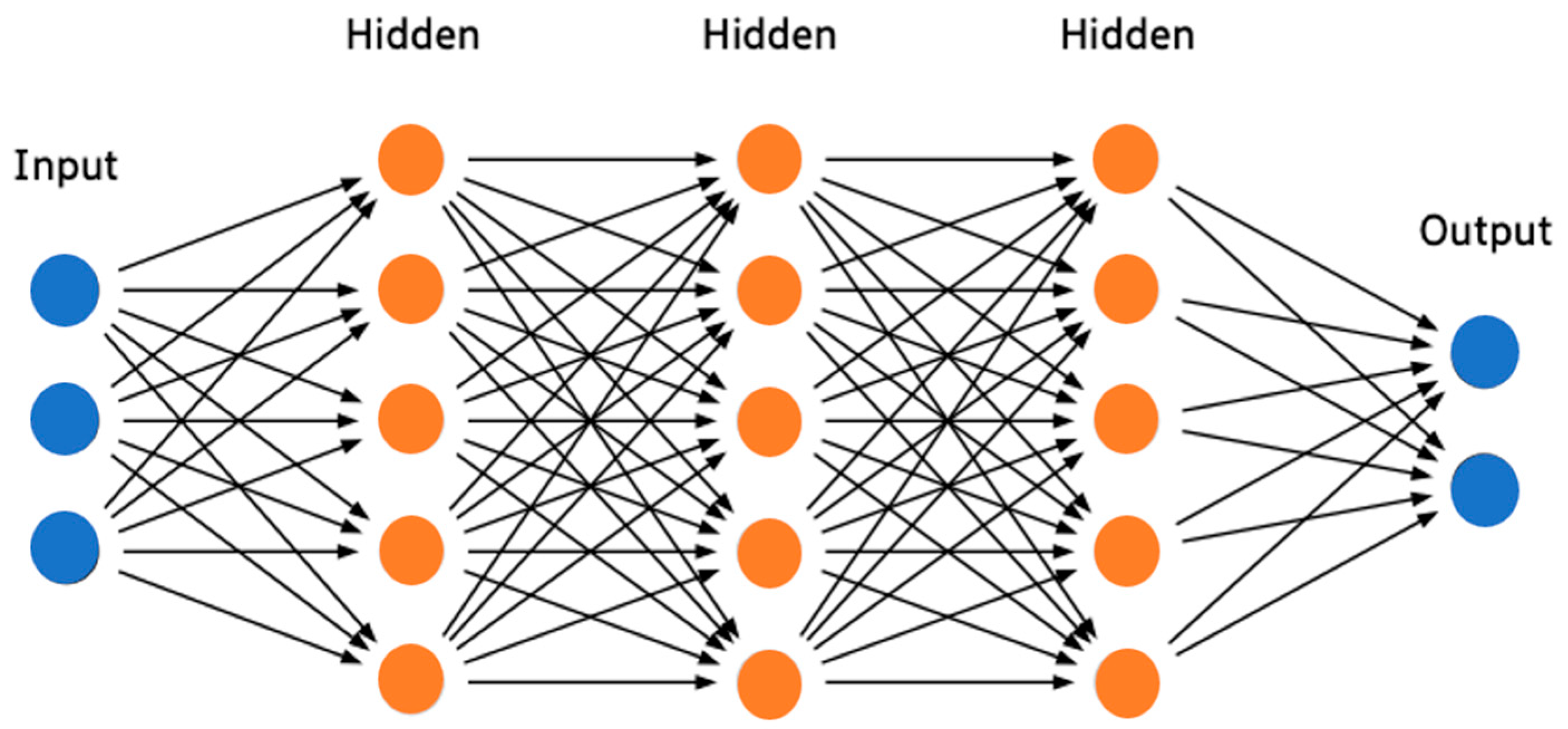
2.2.3. The POD-DNN Method

Deep Neural Networks, being deep multilayer perceptrons (MLPs), can be trained with the back-propagation procedure and model the nonlinear relationship between input and output data. The structure of the DNN is shown in Figure 2.

The formula for a D-layer DNN can be expressed as follows:

$$c=W_{D}O\left(\dots \left(W_{2}O\left(p{W}_1+b_1\right)+b_2\right)\dots \right)+b_D$$

(24)

where $p\in R^m$ and $c\in R^q$ are the input and output vectors of the DNN, and $O$ is the activation function. Take the parameter set of the generated sample as the input data and the coefficient vector $a$ as the output data to train the DNN. The coefficient vector $a\left(p\right)$ can be expressed as in Equation (24), and the final POD-DNN model is as follows:

$$\Psi =\Phi \cdot \left(W_{D}O\left(\dots \left(W_{2}O\left(p{W}_1+b_1\right)+b_2\right)\dots \right)+b_D\right)$$

(25)

In the process of POD-DNN model training, the gradient descent algorithm is often used to minimize the loss function to obtain the best network weights and biases, where the form of the loss function is as follows:

$$Los{s}_{MSE}={\displaystyle \frac{1}{q}}{\displaystyle \sum _{j=1}^q{\left(c_j-{\widehat{c}}_j\right)}^2}$$

(26)

where $c_j$ and ${\widehat{c}}_j$ are the real value of the training data and the predicted value of the POD-DNN model, respectively. The Adam algorithm is used to update the learnable parameters during training. In addition, the proper activation function can improve the learning ability of the network and the accuracy of the model. In this work, the activation function selects the swish to alleviate the gradient disappearance problem.

2.3. Error Analysis

Using $L_2$ norm regularization errors to characterize the global error level, neutron flux and DNP concentration errors are defined as shown in Equations (27) and (28):

$$\Delta {\varphi }_g={\displaystyle \frac{{‖{\varphi }_g^{FOM}-{\varphi }_g^{ROM}‖}_{L_2}}{{‖{\varphi }_g^{FOM}‖}_{L_2}}}$$

(27)

$$\Delta C_j={\displaystyle \frac{{‖C_j^{FOM}-C_j^{ROM}‖}_{L_2}}{{‖C_j^{FOM}‖}_{L_2}}}$$

(28)

In order to analyze the local error in more detail, the absolute error is calculated as follows:

$$\Delta {\varphi }_{g,i}=\left|{\varphi }_{g,i}^{FOM}-{\varphi }_{g,i}^{ROM}\right|$$

(29)

$$\Delta C_{j,i}=\left|C_{j,i}^{FOM}-C_{j,i}^{ROM}\right|$$

(30)

where i is the serial number of the volume unit.

3. Results and Discussion

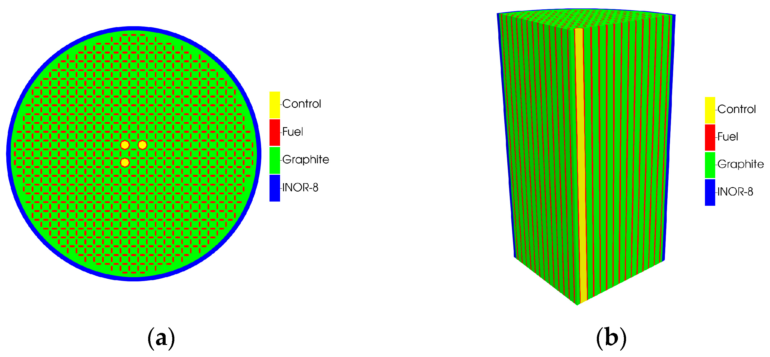
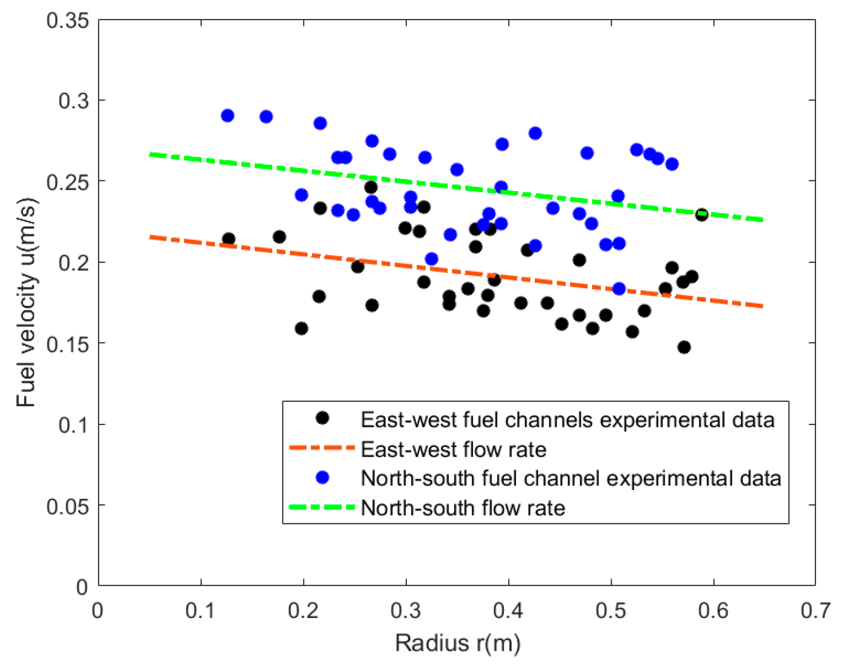
3.1. Benchmark Description

This section establishes a molten salt reactor benchmark, leveraging the experimental data from the Molten Salt Reactor Experiment (MSRE) at Oak Ridge National Laboratory, to systematically evaluate and compare the applicability of the three reduced-order modeling approaches. The MSRE is the first molten salt reactor that was designed, built, and operated by Oak Ridge National Laboratory (ORNL) in the 1960s [30]. It is currently the only available source of molten salt reactor experimental data for liquid fuels.

The structure division of the benchmark is shown in Figure 3. Boundary processing of multi-channel models is one of the challenges in MSR modeling. The entire model is a simplified molten salt reactor core with a height of about 1600.2 mm, and the specific dimensions of each part are shown in

Table 1. Key parameters of molten salt reactor benchmark.

Parameter	Value (cm)
Total height of the model	160.02
Graphite part radius	71.12
Outer reactor vessel radius	73.66
Fuel channel thickness	1.016
Fuel channel width	2.032
Cutout radius at fuel channel corners	0.508
Control rod channel radius	2.347
Radius of fuel channel out of control rod	3.048

. The OpenMC [31,32] code was used to generate the required eight-group cross-sections for the calculation, and the DNP parameters were obtained using the U-235 data in the ORNL report, as shown in

Table 2. Parameters of DNP.

		Total	Group 1	Group 2	Group 3	Group 4	Group 5	Group 6
U-235	$\mathrm{Delayed} \mathrm{neutron} \mathrm{fraction} \beta \left({10}^{-5}\right)$	640.5	21.1	140.2	125.4	252.8	74.0	27.0
	$\mathrm{Decay} \mathrm{constant} \lambda \left(s^{-1}\right)$	-	0.0124	0.0305	0.111	0.301	1.14	3.01

. The fuel flow curve was fitted from the experimental data in the ORNL report [30] to provide a stable flow rate for each fuel channel, as shown in Figure 4.

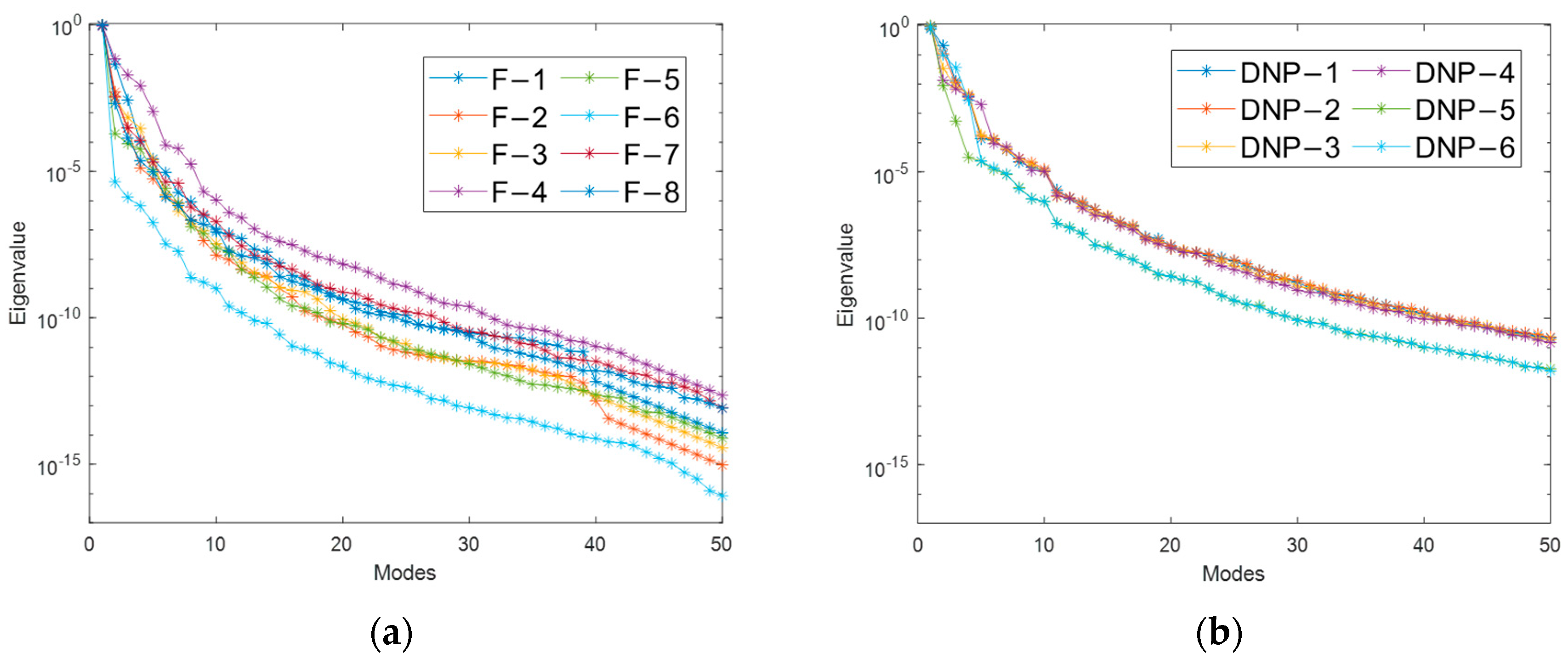
3.2. ROM Parameter Analysis

The mesh size of the molten salt reactor model is about 1.6 million, and the calculation of the full-order model requires more than 500 iteration steps to converge, which takes more than 10 min. For large-scale data analyses, such as uncertainty quantification and core optimization, the computational complexity is considerably high. Due to the high computational cost associated with full-order calculations, there is a need to develop a reduced-order model that can achieve improved accuracy with minimal resource consumption for neutron and DNP calculations in molten salt reactors for uncertainty analysis and core optimization. This approach aims to reduce the resource demands while maintaining calculation precision, especially when working with limited sample inputs. Consequently, the subsequent calculations and analyses are based on a small-sample snapshot set. The Monte Carlo method is one of the most representative computational methods in reactor physics [33,34]. Since the current Monte Carlo method lacks the ability to calculate accurate DNP equations [35], a full-order calculation framework is established based on the open fluid dynamics software OpenFOAM v2206 to generate a set of full-order computing snapshots, which was validated by Cheng et al. [36]. This full-order solver is a multi-physics solver for reactor analysis that is based on the finite volume method (FVM). The snapshot matrices, derived from sampling $D_g$, ${\sum }_{r,g}$, and $\nu {\sum }_{f,g}$ and using them as data for full-order calculations, contain 68 samples each for both the neutron flux and DNP concentration.

To enhance the predictive accuracy and computational efficiency of reduced-order models, systematic hyperparameter optimization of the POD-RBF [37] and POD-DNN [38] frameworks is essential. The prediction model of POD-RBF uses the inverse multiquadric function as the kernel function, and the shape factor c of the kernel function is set to 0.01. The architecture of the POD-DNN prediction model comprises three hidden layers, and their detailed network parameters are presented in

Table 3. The POD-DNN prediction network model’s parameters.

Item	Value	Item	Value
Hidden layer (neutron flux/ DNP concentration)	[128, 128, 64]/[128, 128, 64]	Activation function	Swish
Epochs	2000	LR decay strategy	Exponential decay
Batch size	16	Validation split	20%
Learning rate (LR)	0.001	Early stopping	50 epochs
Dropout rate	0.2	Optimizer	Adam
L2 regularization	0.001

.

The snapshot set is decomposed by the POD method, and the first 50 eigenvalue ratios of the neutron flux and DNP are shown in Figure 5. It can be observed that each group’s modal energy of the neutron flux and DNP vary significantly. Figure 5 indicates that the inclusion of the flow rate increases the complexity of the DNP distribution, requiring a greater number of POD modes to maintain calculation accuracy. The final POD mode number k of each group can be calculated using Equation (10), as shown in

Table 4. The number of POD modes of the neutron flux and DNP concentration for each group.

Parameter	Group	Number of POD Modes
Neutron Flux	1	13
	2	12
	3	12
	4	15
	5	15
	6	18
	7	21
	8	23
DNP concentration	1	18
	2	17
	3	16
	4	14
	5	17
	6	16

. All calculations were normalized and performed on the 13th Gen Intel(R) Core(TM) i9-13980HX 2.20 GHz, 32 GB RAM, and NVIDIA GeForce RTX 4080 Laptop GPU.

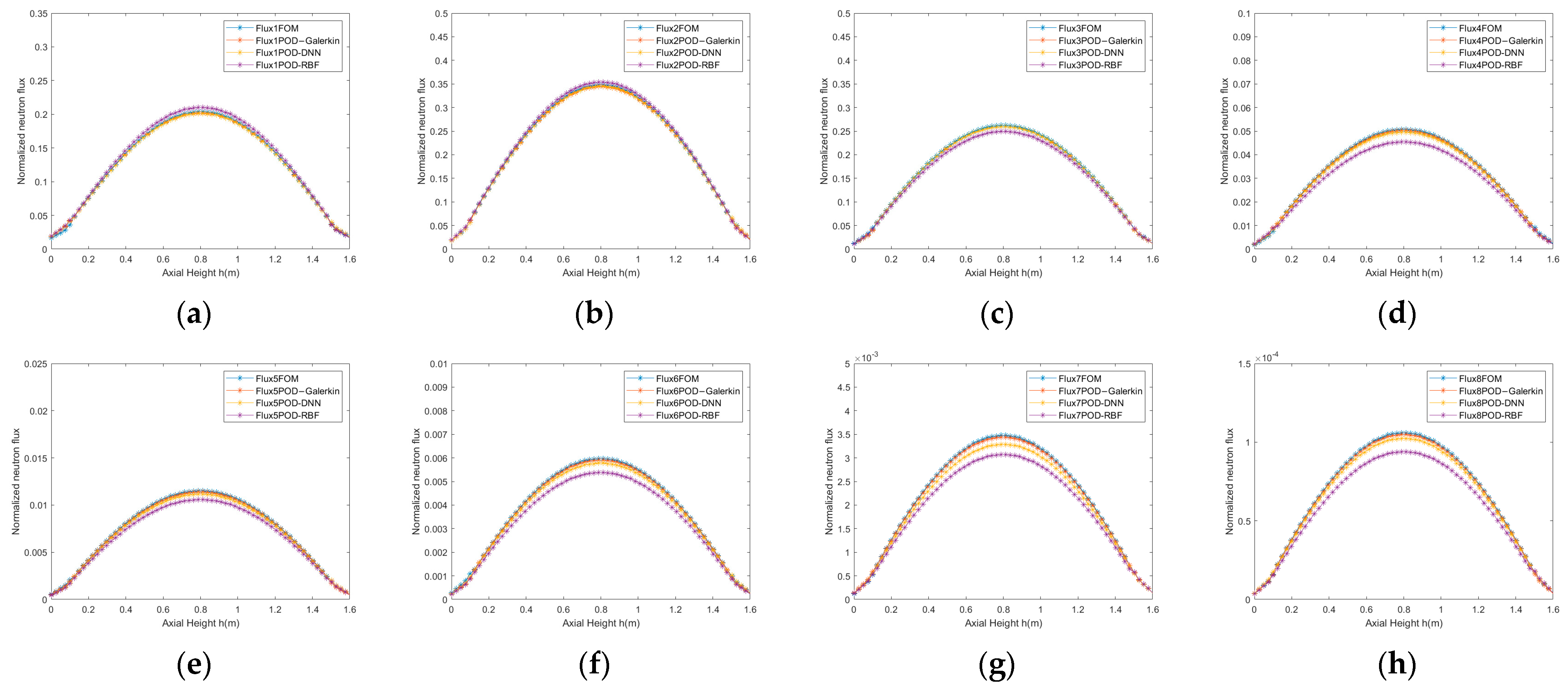
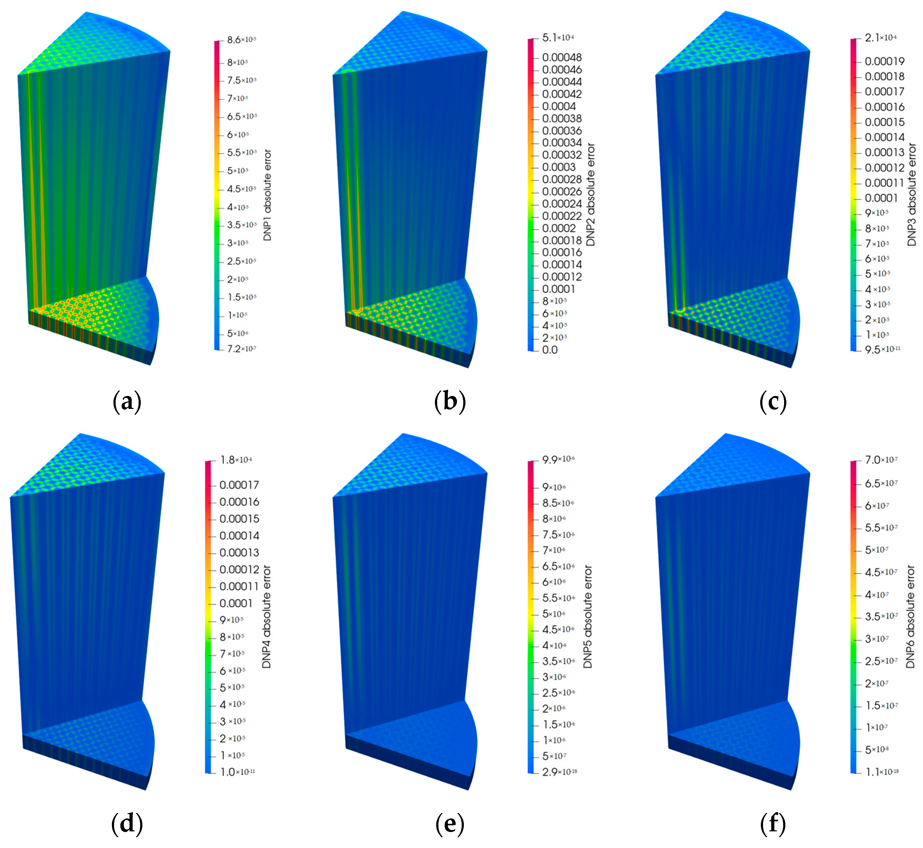
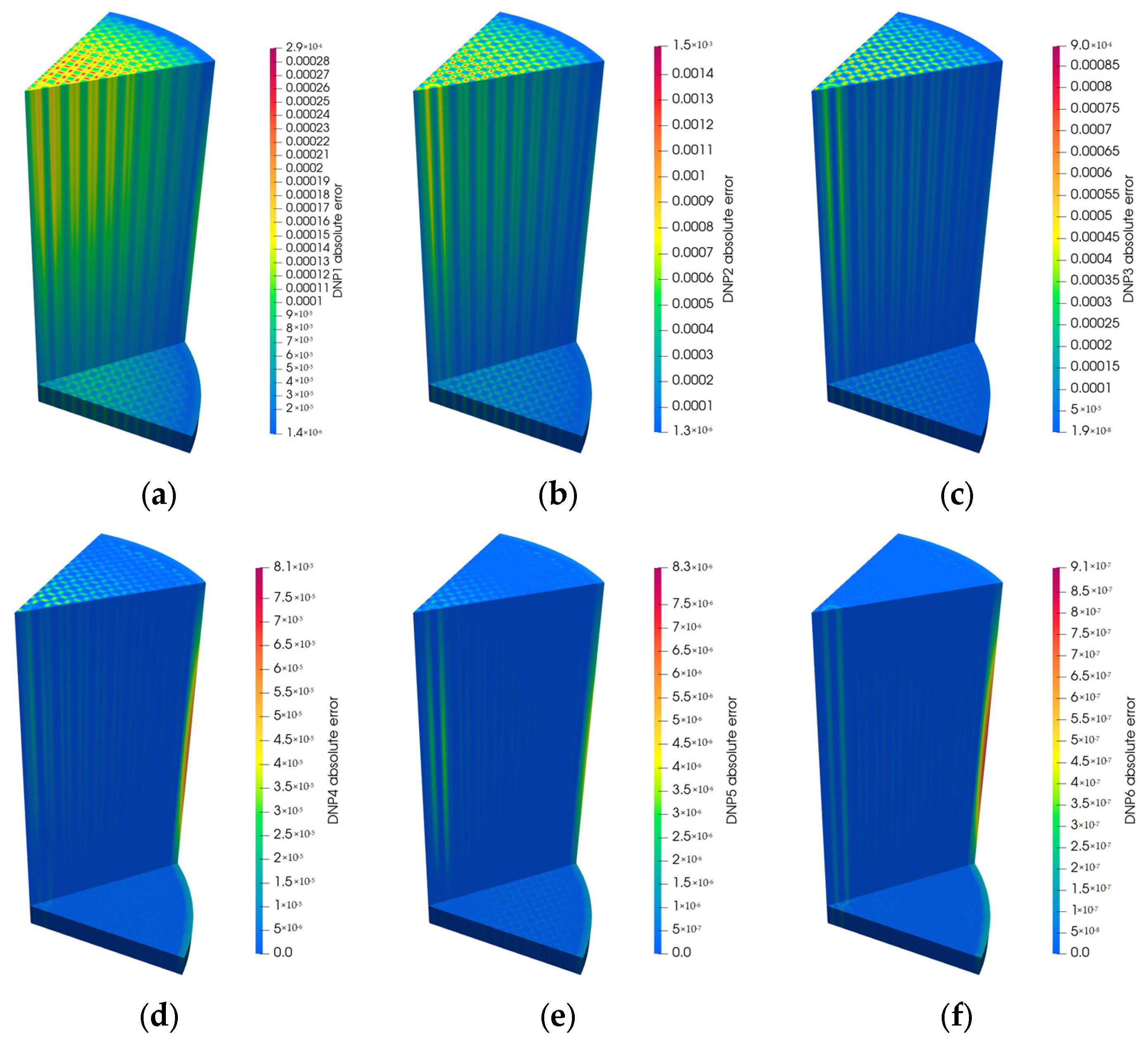
3.3. Accuracy and Performance Analysis

Perturbation sampling of the group constants $D_g$, ${\sum }_{r,g}$, and $\nu {\sum }_{f,g}$ was performed, and we generated 20 samples as test data, starting from ±20% of the standard group constants. The average L₂ errors $\Delta {\varphi }_g$ and $\Delta C_j$ of these 20 test samples are shown in

Table 5. The maximum, minimum, and average L₂ errors of $\Delta {\varphi }_g$ and $\Delta C_j$ for the POD–Galerkin, POD-RBF, and POD-DNN models in a fuel flow case.

Parameter	Method	Max (%)	Min (%)	Avg (%)
$\Delta {\varphi }_g$	POD–Galerkin	1.21 × 10−2	3.68 × 10−3	6.58 × 10−3
	POD-RBF	2.68	1.98 × 10−1	4.08 × 10−1
	POD-DNN	2.25	3.03 × 10−2	7.55 × 10−1
$\Delta C_j$	POD–Galerkin	2.95	2.25 × 10−1	1.01
	POD-RBF	4.58	2.52 × 10−1	2.36
	POD-DNN	3.24	9.81 × 10−2	1.68

, calculated by the POD–Galerkin, POD-RBF, and POD-DNN models, respectively.

According to the results in Table 5, it can be observed that the POD–Galerkin reduced-order model has the highest accuracy in the reconstruction of neutron flux, with an average L₂ error of 0.0065% and a maximum error of 0.012, which is much smaller than the results of the POD-RBF and POD-DNN models. Although the average L₂ error of the POD-DNN model is smaller than the POD-RBF model, its prediction results are volatile. In terms of L₂ errors for the DNP concentration, the average errors of the three models are close to each other. The POD–Galerkin model’s maximum error is slightly lower than those of POD-RBF and POD-DNN, reaching 2.95%. Combining the maximum, minimum, and average error values, the POD–Galerkin model is the best model for predicting the DNP concentration. Figure 6 shows the axial distribution of the neutron flux at a 0.1 m radius for the three reduced-order models for the sample, with the maximum error of the neutron flux L₂ being found in the POD-RBF model.

In Figure 6, errors in the POD-RBF and POD-DNN models occur in the center of the reactor model. The neutron flux error of the POD–Galerkin reduced-order model mainly exists at the boundary. Overall, the POD–Galerkin model has the smallest error, which conforms to the L₂ error results in Table 5.

The distribution of the DNP concentration is of great interest, since the flow velocity of the fuel channel mainly affects it. In the following, the sample with the largest average $\Delta C_j$ error is discussed. The neutron flux absolute errors of this sample are all less than 0.02, the maximum value is 0.018, and all groups’ errors are mainly distributed at the inlet and outlet boundaries. In order to better discuss the local error, Figure 7 shows the three-dimensional distribution of the absolute errors of the DNP concentration.

Based on the results in Figure 7, the absolute errors of the DNP concentration in Figure 7a–d are mainly concentrated at the outlet and inlet borders, while in Figure 7e,f, they are mainly located at the central flow channel. This is due to the fact that in the DNP concentration calculation, the inlet boundary value is calculated according to the special boundary condition in Equation (5), which results in a large error. However, with the increase in the number of energy groups, the decay constant of the DNP concentration increases, resulting in more DNPs remaining in the flow channel, so there will be obvious errors in the flow channel shown, as in Figure 7e,f.

Figure 8 shows the three-dimensional distribution of the absolute error of the concentration of DNPs for the test sample, computed by the POD-RBF model. Compared with the results of the POD–Galerkin reduced-order model, the POD-RBF model’ results have slightly larger errors.

The error of the POD-RBF model is primarily concentrated at the outlet and boundaries, as can be seen from Figure 8. This is due to the fact that the POD mode decomposition only retains a limited number of dominant modes, while the intricate details at the boundaries are often represented in higher-order modes. Consequently, the POD method may not sufficiently capture the complex variations in the data. At the same time, the POD-RBF model is a pure function approximation model, which does not need to solve PDEs, so the boundary behavior is not shown to be explicitly considered, resulting in the prediction value of the POD-RBF model on the boundary not matching the full-order model. Compared with Figure 8, the maximum error value of the POD-RBF model is larger than that in the POD–Galerkin model, but there are fewer regions that generate errors, so the two models perform similarly in terms of the global error.

Figure 9 shows the three-dimensional distribution of the absolute error of the concentration of DNPs for the test sample, computed by the POD-DNN model.

Figure 9 shows that the error distribution of the POD-DNN model is similar to that of the POD-RBF model, and errors are mainly generated at the boundary. Both the RBF and DNN serve as “black box” surrogate models; hence, the underlying reasons for their similar error distributions can be attributed to this shared characteristic.

When evaluating the applicability of the reduced-order model, the calculation cost of the reduced-order model should be considered in addition to the calculation accuracy.

Table 6. Average calculation time and acceleration rate for three reduced-order models.

Method	FOM Calculation Time (s)	ROM Calculation Time (s)	Acceleration Rate
POD–Galerkin	649.72	0.358	1814
POD-RBF	649.72	0.627	1036
POD-DNN	649.72	0.75	866

shows the calculation time and acceleration ratio of the three reduced-order models. The POD–Galerkin has the highest acceleration ratio at 1814, followed by POD-RBF at 1036.

In addition, the extrapolation ability of the three reduced-order models was tested. We performed perturbation sampling on the group constants $D_g$, ${\sum }_{r,g}$, and $\nu {\sum }_{f,g}$ and generated a total of 13 groups of perturbation parameters, ranging from ±20 to ±25% of the standard group constants. These samples’ parameters were outside the range of parameters that were used to generate the snapshot matrices $M_{{\varphi }_g}$ and $M_{C_j}$. Figure 10 illustrates the multi-energy group average L₂ error for $\Delta {\varphi }_g$ and $\Delta C_j$ across the 13 test samples.

For the input parameters that deviate from the distribution of the training data, Figure 10 clearly illustrates that the reduced-order model based on POD-RBF fails to accurately predict the neutron flux and DNP concentration. Specifically, the maximum L₂ error for the neutron flux across multiple energy groups is 36.7%, while the maximum error for the DNP concentration reaches 19.8%. This is because the response of the radial basis function will decay rapidly with the increase in the distance between the input parameter and the center point. When the input data are far away from the central region of the training set, the hidden layer activations will approach zero, causing the model output to only depend on a few unattenuated nodes, which will bias the prediction. At the same time, the output layer of RBF is usually a linear combination of the response to the hidden layer, which lacks the ability to model the nonlinear relationship in the extrapolated region. The reduced-order model based on POD-DNN outperforms the POD-RBF model, with the errors in neutron flux and DNP concentration remaining below 15%. The DNN model uses multilayer nonlinear transformation to learn complex patterns and theoretically has a strong extrapolation ability. The construction of the three models is based on small sample set. Usually, the training of neural networks requires a very large amount of data, so insufficient samples are the main reason for the poor performance of the POD-DNN model’s extrapolation ability. The reduced-order model based on the POD–Galerkin methods showed an excellent extrapolation ability, with a maximum average L₂ error of 5.12% for the neutron flux and 6.04% for the DNP concentration. This is due to the Galerkin method projecting the original equation onto a low-dimensional space of the basic POD span, effectively preserving the physical structure of the original equation. This physics-based constraint makes the model conform to the basic equation structure when the parameters are extrapolated and avoids over-dependence on the training data.

4. Conclusions

To address computational efficiency challenges in solving neutron multi-group diffusion equations and DNP conservation equations for molten salt reactors, an intrusive reduced-order model based on the POD–Galerkin methodology for molten salt reactors was developed. Two representative non-intrusive reduced-order modeling approaches were also introduced, and the POD-RBF and POD-DNN frameworks were established through hyperparameter adjustment. Through systematic parameter perturbation experiments on the fuel parameters $D_g$, ${\sum }_{r,g}$, and $\nu {\sum }_{f,g}$, the applicability levels of these three models were comprehensively investigated, with a quantitative evaluation of their acceleration ratios. The numerical simulation results demonstrated the following:

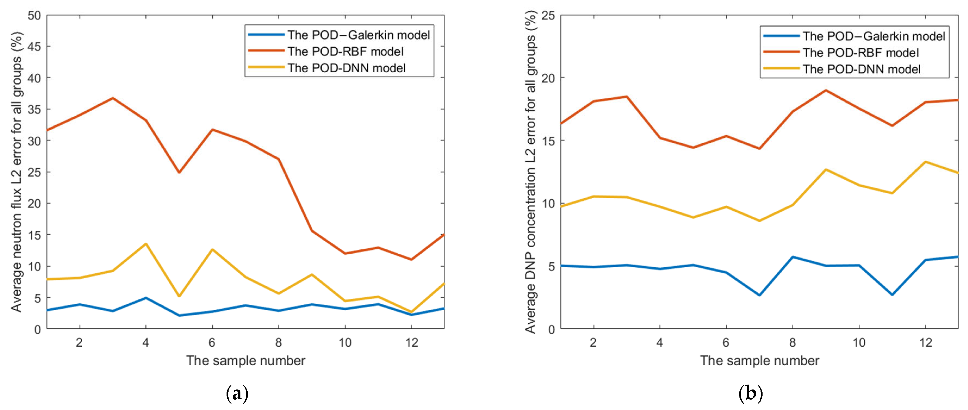
• For reduced-order calculations of the neutron flux and DNP concentration under small-sample conditions, the POD–Galerkin model demonstrates superior computational accuracy compared to the POD-RBF and POD-DNN models, with average L₂ errors of less than 0.00658% for the neutron flux and 1.01% for the DNP concentration. And the POD–Galerkin model exhibits excellent extrapolation capabilities and maintains an L₂ error of less than 6.04% when the test samples exceed the range of the snapshot samples.
• All three reduced-order models can effectively improve the computational efficiency, and the POD–Galerkin model has an acceleration ratio of about 1800.

In summary, the POD–Galerkin method can improve the calculation efficiency while maintaining a high calculation accuracy and is more suitable for the construction of a reduced-order model for molten salt reactors in the case of small samples. The results of the applicability analysis provide important and actionable insights for the development of a robust, efficient, and accurate computational framework tailored for neutron computational analysis and design optimization in molten salt reactors. On this basis, further research into the theory and methodology of neutron transport model reduction with enhanced accuracy can be conducted. In future work, it will be essential to analyze and optimize the reduced-order model for the transient conditions of molten salt reactors, thereby fulfilling the requirements for accurate operational prediction and analysis of molten salt reactors.

References

1. Song, S.; Cheng, M.; Lin, M. Development and application of multi-scale thermal fluid coupling program for molten salt cooled fast reactor based on RELAP5 and sub-channel program. Nucl. Tech. 2022, 45, 070602. [Google Scholar] [CrossRef]
2. Zong, Z.-W.; Cheng, M.-S.; Yu, Y.-C.; Dai, Z.-M. A multithreaded parallel upwind sweep algorithm for the SN transport equations discretized with discontinuous finite elements. Nucl. Sci. Tech. 2023, 34, 200. [Google Scholar] [CrossRef]
3. Guo, Z.; Zhou, J.; Zhang, D.; Chaudri, K.S.; Tian, W.; Su, G.; Qiu, S. Coupled neutronics/thermal-hydraulics for analysis of molten salt reactor. Nucl. Eng. Des. 2013, 258, 144–156. [Google Scholar] [CrossRef]
4. Zuo, X.-D.; Cheng, M.-S.; Dai, Y.-Q.; Yu, K.-C.; Dai, Z.-M. Flow field effect of delayed neutron precursors in liquid-fueled molten salt reactors. Nucl. Sci. Tech. 2022, 33, 96. [Google Scholar] [CrossRef]
5. Mathieu, L.; Heuer, D.; Brissot, R.; Garzenne, C.; Le Brun, C.; Lecarpentier, D.; Liatard, E.; Loiseaux, J.M.; Méplan, O.; Merle-Lucotte, E.; et al. The thorium molten salt reactor: Moving on from the MSBR. Prog. Nucl. Energy 2006, 48, 664–679. [Google Scholar] [CrossRef]
6. Lin, M.; Cheng, M.; Cai, X.; Dai, Z.-M. Applicability analysis of reduced order modeling methods for fluid dynamics in molten salt reactor. Nucl. Tech. 2024, 47, 090604. [Google Scholar] [CrossRef]
7. Berkooz, G.; Holmes, P.; Lumley, J.L. The Proper Orthogonal Decomposition in the Analysis of Turbulent Flows. Annu. Rev. Fluid Mech. 1993, 25, 539–575. [Google Scholar] [CrossRef]
8. Noack, B.R. Turbulence, Coherent Structures, Dynamical Systems and Symmetry. AIAA J. 2013, 51, 2991. [Google Scholar] [CrossRef]
9. Abrate, N.; Dulla, S.; Pedroni, N. A non-intrusive reduced order model for the characterisation of the spatial power distribution in large thermal reactors. Ann. Nucl. Energy 2023, 184, 109674. [Google Scholar] [CrossRef]
10. Benner, P.; Gugercin, S.; Willcox, K. A Survey of Projection-Based Model Reduction Methods for Parametric Dynamical Systems. SIAM Rev. 2015, 57, 483–531. [Google Scholar] [CrossRef]
11. Raffel, C.; Shazeer, N.; Roberts, A.; Lee, K.; Narang, S.; Matena, M.; Zhou, Y.; Li, W.; Liu, P.J. Exploring the limits of transfer learning with a unified text-to-text transformer. J. Mach. Learn. Res. 2020, 21, 140. [Google Scholar] [CrossRef]
12. Bei, X.; Dai, Y.; Yu, K.; Cheng, M. Three-Dimensional Surrogate Model Based on Back-Propagation Neural Network for Key Neutronics Parameters Prediction in Molten Salt Reactor. Energies 2023, 16, 4044. [Google Scholar] [CrossRef]
13. Buchan, A.G.; Pain, C.C.; Fang, F.; Navon, I.M. A POD reduced-order model for eigenvalue problems with application to reactor physics. Int. J. Numer. Methods Eng. 2013, 95, 1011–1032. [Google Scholar] [CrossRef]
14. Sartori, A.; Baroli, D.; Cammi, A.; Chiesa, D.; Luzzi, L.; Ponciroli, R.; Previtali, E.; Ricotti, M.E.; Rozza, G.; Sisti, M. Comparison of a Modal Method and a Proper Orthogonal Decomposition approach for multi-group time-dependent reactor spatial kinetics. Ann. Nucl. Energy 2014, 71, 217–229. [Google Scholar] [CrossRef]
15. German, P.; Ragusa, J.C. Reduced-order modeling of parameterized multi-group diffusion k-eigenvalue problems. Ann. Nucl. Energy 2019, 134, 144–157. [Google Scholar] [CrossRef]
16. Prince, Z.M.; Ragusa, J.C. Parametric uncertainty quantification using proper generalized decomposition applied to neutron diffusion. Int. J. Numer. Methods Eng. 2019, 119, 899–921. [Google Scholar] [CrossRef]
17. Ostrowski, Z.; Białecki, R.A.; Kassab, A.J. Solving inverse heat conduction problems using trained POD-RBF network inverse method. Inverse Probl. Sci. Eng. 2008, 16, 39–54. [Google Scholar] [CrossRef]
18. Das, A.; Khoury, A.; Divo, E.; Huayamave, V.; Ceballos, R.; Eaglin, R.; Kassab, A.; Payne, A.; Yelundur, V.; Seigneur, H. Real-Time Thermomechanical Modeling of PV Cell Fabrication via a POD-Trained RBF Interpolation Network. Comput. Model. Eng. Sci. 2020, 122, 757–777. [Google Scholar] [CrossRef]
19. Elzohery, R.; Roberts, J. Exploring Transient, Neutronic, Reduced-Order Models using DMD/POD-Galerkin and Data-Driven DMD; EDP Sciences: Les Ulis, France, 2020. [Google Scholar]
20. Hasan, M.D.A.; Balasubadra, K.; Vadivel, G.; Arunfred, N.; Ishwarya, M.V.; Murugan, S. IoT-Driven Image Recognition for Microplastic Analysis in Water Systems using Convolutional Neural Networks. In Proceedings of the 2024 2nd International Conference on Computer, Communication and Control (IC4), Indore, India, 8–10 February 2024; pp. 1–6. [Google Scholar]
21. Kang, H.; Tian, Z.; Chen, G.; Li, L.; Wang, T. Application of POD reduced-order algorithm on data-driven modeling of rod bundle. Nucl. Eng. Technol. 2022, 54, 36–48. [Google Scholar] [CrossRef]
22. Massone, M.; Gabrielli, F.; Rineiski, A. A genetic algorithm for multigroup energy structure search. Ann. Nucl. Energy 2017, 105, 369–387. [Google Scholar] [CrossRef]
23. Wei, C.; Ooka, R.; Zhang, B.; Zhou, Q. Predicting Unsteady Indoor Temperature Distributions by POD-DNN. E3S Web Conf. 2022, 356, 04028. [Google Scholar] [CrossRef]
24. Kiegiel, K.; Chmielewska-Śmietanko, D.; Herdzik-Koniecko, I.; Miśkiewicz, A.; Smoliński, T.; Rogowski, M.; Ntang, A.; Rotich, N.K.; Madaj, K.; Chmielewski, A.G. The Future of Nuclear Energy: Key Chemical Aspects of Systems for Developing Generation III+, Generation IV, and Small Modular Reactors. Energies 2025, 18, 622. [Google Scholar] [CrossRef]
25. Panico, D.M. Development of a C++ tool for Reduced Order Modelling of Molten Salt Fast Reactor multiphysics: Sensitivity Analysis application. Doctoral Dissertation, Politecnico di Torino, Turin, Italy, 2019. [Google Scholar]
26. Qian, H.; Chen, G.; Liu, D.; Yu, Y.; Zhang, Y.; Zhang, L.; Li, J. Development of a non-intrusive ROM for 5 × 5 rod bundles of PWR using small sample data. Ann. Nucl. Energy 2025, 217, 111347. [Google Scholar] [CrossRef]
27. Zhang, Y.; Li, W.; Peng, S.; Li, J.; Wang, T.; He, Q.; Wang, T.; Lu, H.; Zeng, L. Enhancing uncertainty analysis: POD-DNNs for reduced order modeling of neutronic transient behavior. Nucl. Eng. Des. 2025, 435, 113969. [Google Scholar] [CrossRef]
28. Sirovich, L. Turbulence and the dynamics of coherent structures. II. Symmetries and transformations. Q. Appl. Math. 1987, 45, 573–582. [Google Scholar] [CrossRef]
29. Liang, Y.C.; Lin, W.Z.; Lee, H.P.; Lim, S.P.; Lee, K.H.; Sun, H. Proper Orthogonal Decomposition and its Applications—Part II: Model Reduction for Mems Dynamical Analysis. J. Sound Vib. 2002, 256, 515–532. [Google Scholar] [CrossRef]
30. Haubenreich, P.N.; Engel, J.R.; Prince, B.E.; Claiborne, H.C. Msre Design and Operations Report. Part III. Nuclear Analysis; Oak Ridge National Lab. (ORNL): Oak Ridge, TN, USA, 1964; p. 204.
31. Romano, P.K.; Forget, B. The OpenMC Monte Carlo particle transport code. Ann. Nucl. Energy 2013, 51, 274–281. [Google Scholar] [CrossRef]
32. Romano, P.K.; Horelik, N.E.; Herman, B.R.; Nelson, A.G.; Forget, B.; Smith, K. OpenMC: A state-of-the-art Monte Carlo code for research and development. Ann. Nucl. Energy 2015, 82, 90–97. [Google Scholar] [CrossRef]
33. Kępisty, G.; Oettingen, M.; Stanisz, P.; Cetnar, J. Statistical error propagation in HTR burnup model. Ann. Nucl. Energy 2017, 105, 355–360. [Google Scholar] [CrossRef]
34. Oettingen, M.; Kim, J. Detection of Numerical Power Shift Anomalies in Burnup Modeling of a PWR Reactor. Sustainability 2023, 15, 3373. [Google Scholar] [CrossRef]
35. Vieira, T.A.S.; Carvalho, Y.M.; Gonçalves, R.C.; de Almeida Carvalho, K.; Silva, V.V.A.; Barros, G.P.; Santos, A.A.C.d. Proposition of a small molten salt modular reactor utilizing fine-mesh 1:1 coupled calculations—Part I. Ann. Nucl. Energy 2025, 213, 111079. [Google Scholar] [CrossRef]
36. Cheng, M.-S.; Dai, Z.-M. Development of a three dimension multi-physics code for molten salt fast reactor. Nucl. Sci. Tech. 2014, 25, 66–76. [Google Scholar] [CrossRef]
37. Naha, S.; Das, D.K. Radial basis function neural network controller for power control of molten salt breeder reactor of nuclear power plant. Ann. Nucl. Energy 2024, 195, 110160. [Google Scholar] [CrossRef]
38. Foad, B.; Elzohery, R.; Novog, D.R. Demonstration of combined reduced order model and deep neural network for emulation of a time-dependent reactor transient. Ann. Nucl. Energy 2022, 171, 109017. [Google Scholar] [CrossRef]
Figure 1. Reduced-order model workflow.
Energies 18 01893 g001
Figure 2. Structure of DNN.
Energies 18 01893 g002
Figure 3. The molten salt reactor benchmark’s structure: (a) material structure (top view); (b) material structure (side cut).
Energies 18 01893 g003
Figure 4. The fuel velocity distribution.
Energies 18 01893 g004
Figure 5. Normalized modal eigenvalue curves: (a) neutron flux; (b) DNP concentration.
Energies 18 01893 g005
Figure 6. Neutron flux distribution of axial results at 0.1 m radius: (a) Group 1; (b) Group 2; (c) Group 3; (d) Group 4; (e) Group 5; (f) Group 6; (g) Group 7; (h) Group 8.
Energies 18 01893 g006
Figure 7. DNP concentration absolute error distribution with the POD–Galerkin reduced-order model: (a) Group 1; (b) Group 2; (c) Group 3; (d) Group 4; (e) Group 5; (f) Group 6.
Energies 18 01893 g007
Figure 8. DNP concentration absolute error distribution with the POD-RBF reduced-order model: (a) Group 1; (b) Group 2; (c) Group 3; (d) Group 4; (e) Group 5; (f) Group 6.
Energies 18 01893 g008
Figure 9. DNP concentration relative error distribution with the POD-DNN reduced-order model: (a) Group 1; (b) Group 2; (c) Group 3; (d) Group 4; (e) Group 5; (f) Group 6.
Energies 18 01893 g009
Figure 10. (a,b) Multi-energy group average L 2 error of Δ ϕ g and Δ C j for three methods, with parameters ranging from ±20 to ±25% of standard group constants.
Energies 18 01893 g010