In this study, through simulations of natural convection in a cavity in both two and three dimensions, we first demonstrate that our Fokker–Planck central moment-based collision model can be utilized for the accurate simulation of thermal convective flows. The physics of this problem is modulated primarily by the Rayleigh number
, which represent the relative effects of buoyancy forces to the opposing effects of viscous and thermal diffusions, as well as the Prandtl number
, which characterizes the relative strength of viscous to thermal diffusion. We will compare the numerical results of simulations using our FPC-LBMs, across a range of Rayleigh numbers at a fixed
for air with a variety of references including both prior numerical solutions [
46,
61,
62,
63,
64,
65] and experimental measurements [
66,
67,
68,
69]. In two dimensions, we will also perform a grid convergence study in obtaining the Nusselt numbers in the simulations involving higher
. It is well known that, above a Rayleigh number of about
, the flow becomes transitional and turbulent natural convection characteristics emerge, and the use of adequately refined grids and a sufficient duration for the collection of statistics are required. While, in the 2D case, we will consider
as high as
, since the standard LBM is restricted to uniform grids and, due to the limited availability of computing resources, we will restrict
to be up to
in 3D, in future work, we plan to incorporate grid clustering techniques using coordinate transformations to simulate higher
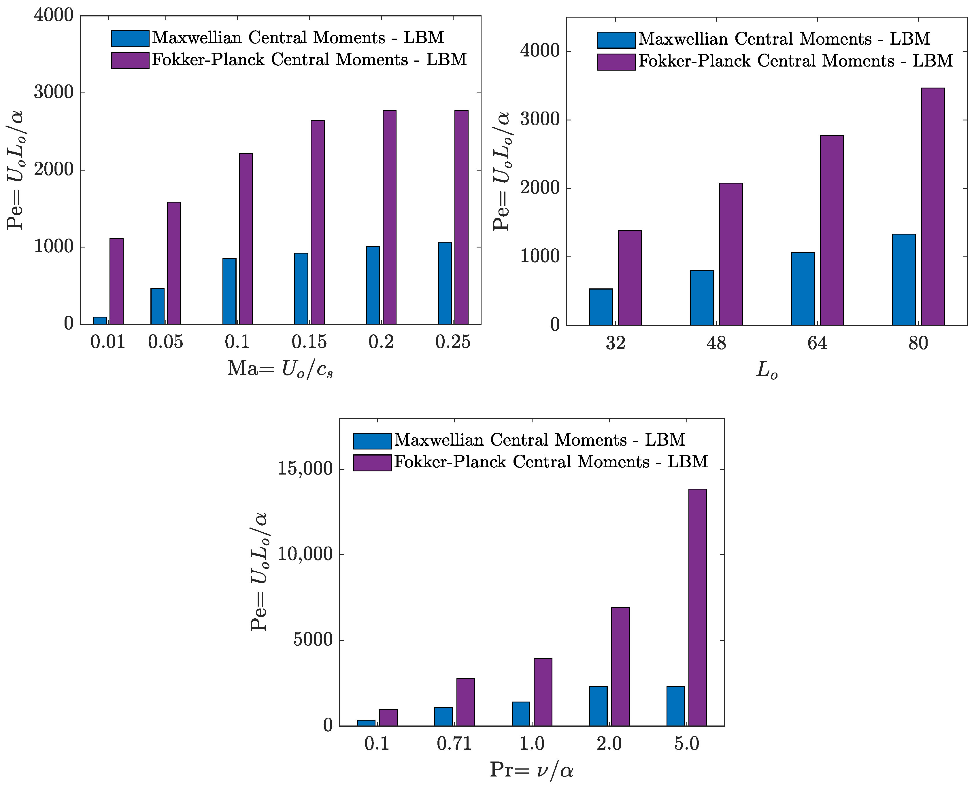
in 3D. In addition, we will perform a comparative numerical stability study to show the benefits of using the FPC-LBM over the state-of-the-art LBM utilizing the central moment-based collision models based on the Maxwell distribution, which has been used in several recent investigations [
46,
47,
48,
49,
50], for simulations of mixed thermal convection driven by buoyancy forces and an imposed shear.
6.1. Natural Convection in a Square Cavity
We perform simulations of the canonical natural convection in a square cavity benchmark problem at various
to provide a validation of the Fokker–Planck central moment-based collision model applied to both the distribution functions solving for fluid flow as well as the temperature field. Applying and quantitatively studying this collision model to the second distribution function has not been performed before and is a natural extension of our previous FPC-LBM for hydrodynamics [
33]. In essence, the 2D FPC-LBM for fluid motions is given in
Appendix A and another 2D FPC-LBM for energy transport provided in
Appendix B. A schematic diagram of the problem set up in a square cavity of side length
is shown in
Figure 1.
First, we now briefly mention the boundary conditions utilized for this problem whose implementation details are given, for example, in Ref. [
41]. The no-slip condition is applied on all four walls for the fluid velocity using the half-way bounce back scheme for the distribution function
. On the other hand, the upper and lower walls have zero temperature gradient (adiabatic) which are also specified using a half-way bounce back method for
, while the left wall has a constant and uniform hot temperature,
, and the right wall has a constant and uniform cold temperature applied,
, and they are implemented using the half-way anti-bounce back approach for the distribution function
. As is standard in performing simulations using LB schemes, we will utilize the lattice units in setting up the parameters of the problem, i.e., unit lattice spacing and time step are used (see Ref. [
41]). Then, the characteristic length or the side of the square cavity
determines the number of grid nodes used and the characteristic velocity is fixed to
so that the Mach number is relatively small and the resulting flow can be regarded as incompressible. Furthermore, the characteristic force per unit mass used to simulate gravity is
. The hot temperature imposed on the left wall is fixed at
, while the cold temperature on the right wall is set at
in lattice units.
The FPC-LBM used to solve the temperature field is coupled to that for the hydrodynamics via an external body force due to buoyancy. Under the usual Boussinesq approximation, we can write the vertical component of the force as
, and its horizontal component as
, so that
is the force locally impressed on the fluid. Here,
is the thermal expansion coefficient,
T is the local temperature, and the mean temperature defined as
represents the characteristic temperature scale. We perform simulations across a range of Rayleigh numbers
at a fixed Prandtl number
, which are defined as
where
and
are the kinematic viscosity (which controls the momentum diffusivity) and thermal diffusivity, respectively, and they are related to the relaxation parameters used in the collision steps (see the last paragraphs of
Appendix A and
Appendix B for details). Here, unless otherwise stated, we fix
as
corresponding to that of air.
The heat transfer rate is determined by the dimensionless Nusselt number, which requires an estimation of the normal temperature gradient on walls. Since we use a half-way bounce back boundary technique, our true boundary location is half-way located between the first fluid node and that of the ghost node inside the wall. To that end, we utilize a second-order Lagrange interpolating polynomial for unequally spaced data to estimate the first derivative of the temperature field, which reads as
where the wall location is at
, and the first two fluid nodes are located at
and
, respectively. Subsequently, expressing the function values corresponding to the temperature on the wall and the temperature at the first two fluid nodes as
,
, and
, respectively, and then evaluating the derivative at
, we obtain
Then, the local Nusselt number
at the hot wall, where
, is defined as
and the average Nusselt number
at this wall as
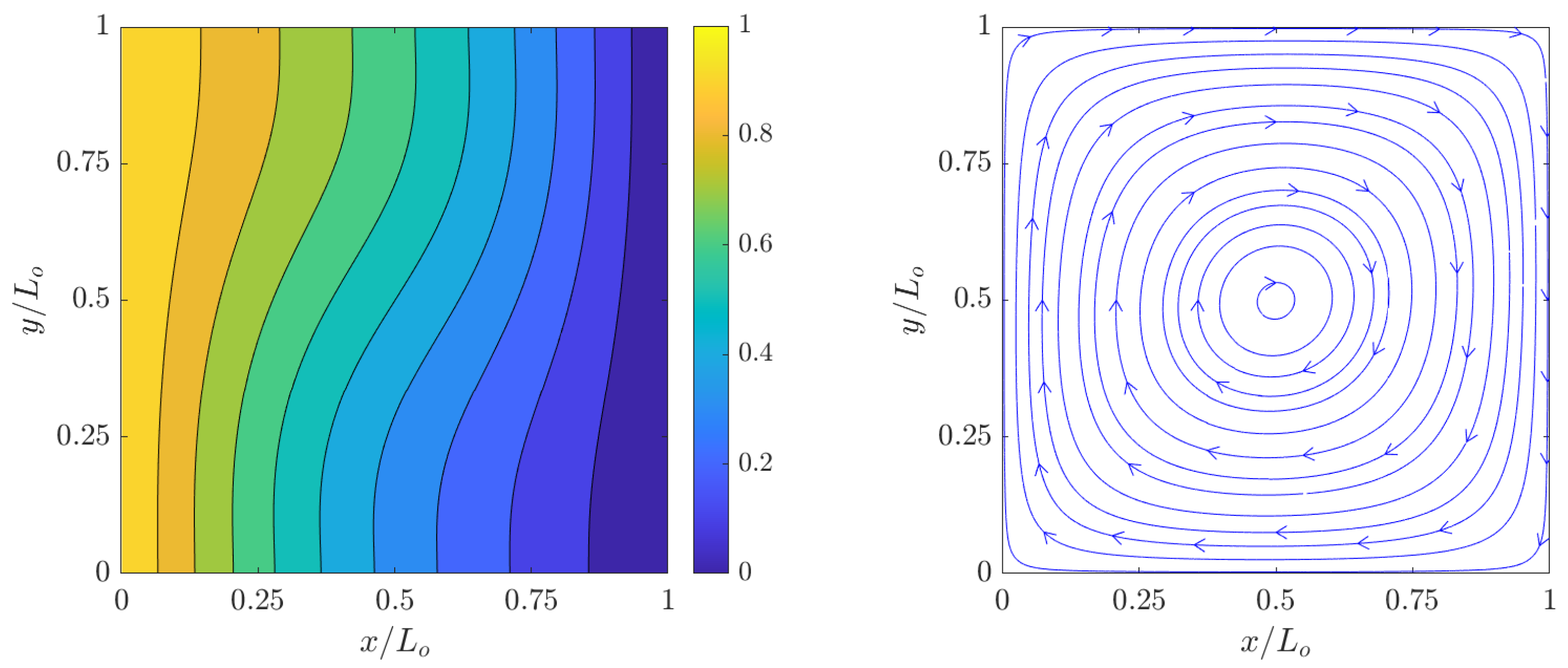
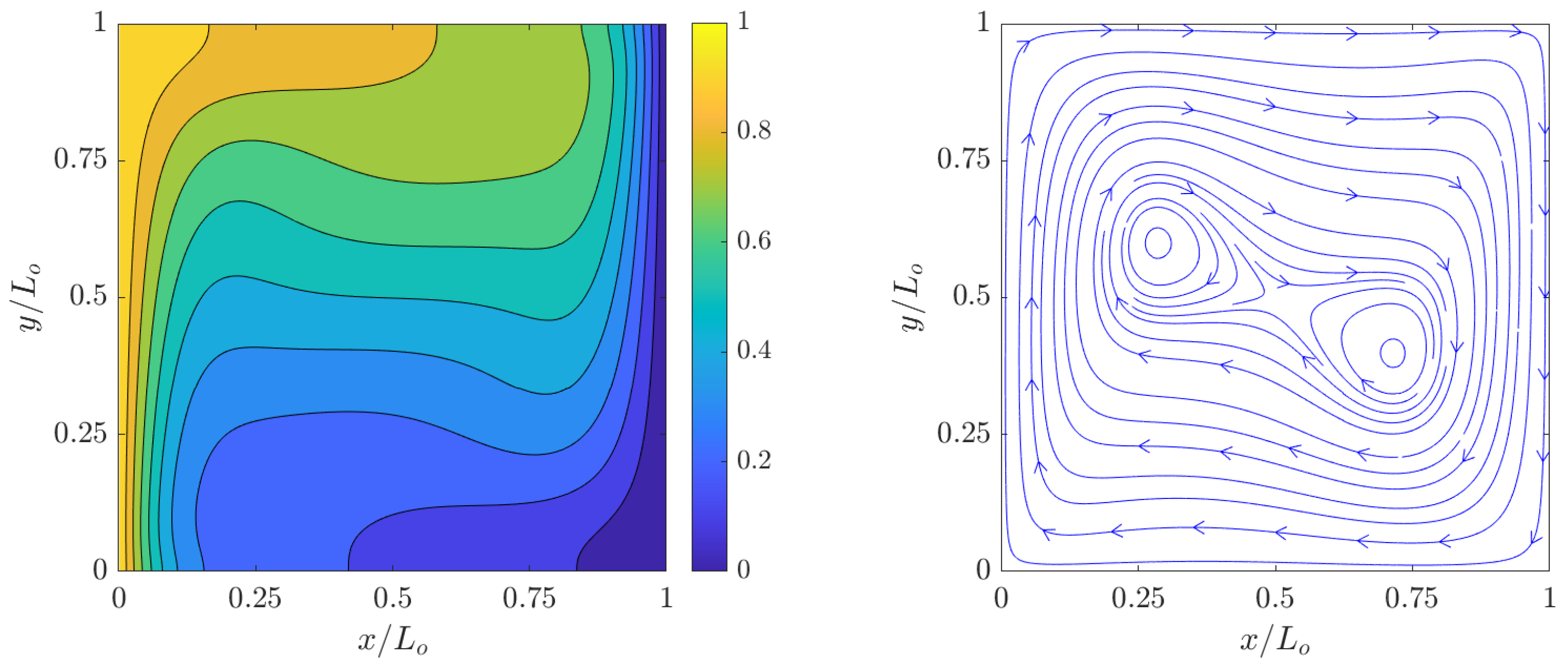
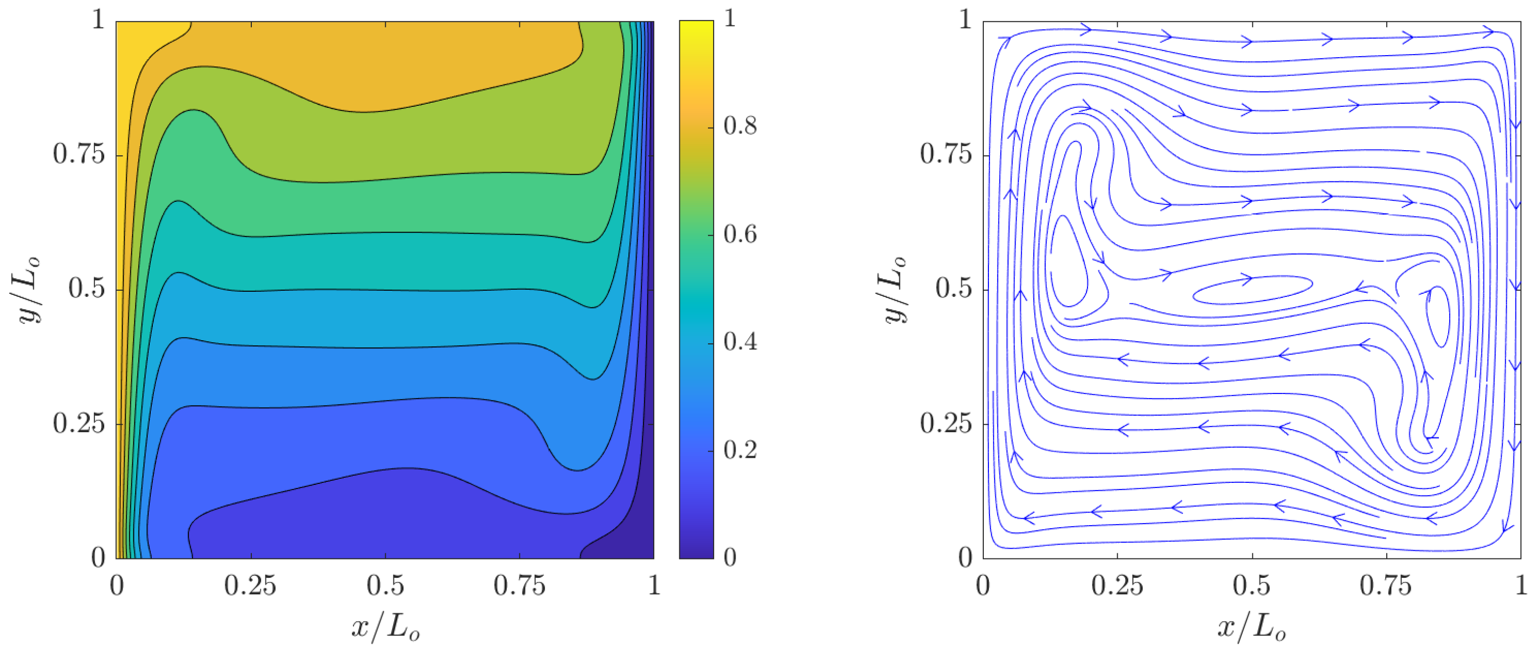
The simulation results of the dimensionless temperature contours
) and streamlines for the velocity fields at steady state computed using the 2D FPC-LBMs using a resolution of
grid nodes for
,
,
, and
are shown in
Figure 2,
Figure 3,
Figure 4 and
Figure 5. Clearly, as
increases, the temperature boundary layers at the hot and cold walls becomes thinner with a concomitant increase in the natural convective flows in their vicinities; moreover, as the relative effects of the buoyancy forces over the counteracting viscous forces and thermal diffusion increase, the vortical structures, which are formed as a result of clockwise flow circulation due to thermal exchanges between the side walls, become increasingly more complex. These observations are found to be qualitatively similar to those shown in the literature.
However, to obtain a more quantitative comparison, next, we look at the temperature profiles along the horizontal centerlines at
for the above low-to-moderate Rayleigh numbers.
Figure 6 shows those profiles computed using the FPC-LBMs overlaid with the prior reference numerical data of Ref. [
63] for
through
. Good agreement is seen for these cases.
Moreover, to obtain further validation quantitatively, some relevant parameters such as the Nusselt numbers (maximum, minimum, and average) along the heated wall and maximum natural convection velocity components and their locations are computed using the 2D FPC-LBMs and then compared with reference data available in the literature. The definitions of those parameters are as follows:
is the maximum horizontal velocity on the vertical centerline of the cavity and
is the maximum vertical velocity on the horizontal centerline of the cavity with their locations given as
y and
x, respectively;
,
, and
are the average Nusselt number, maximum Nusselt number, and minimum Nusselt number, respectively, along the hot wall at
, while the location of the last two quantities is identified to be at
y. Here, the coordinate locations are normalized by the characteristic length
. The results for these parameters at
,
,
, and
are tabulated in
Table 2,
Table 3,
Table 4 and
Table 5, where the comparisons are made against the prior numerical solutions reported in Refs. [
46,
61,
62,
63]. Evidently, the FPC-LBM results are generally in good quantitative agreement with the available data in the literature.
Moving beyond the moderate Rayleigh numbers, from
at
to higher values at
and
, it is expected that, to resolve the progressively thinner boundary layers, resolutions greater than
grid points are necessary to resolve the heat transfer rates adequately across the heated wall. Hence, we performed a systematic grid convergence study in the prediction of the Nusselt numbers at
,
, and
for a wide range of following grid resolutions:
,
,
,
,
,
, and
. All the simulations were run for
time steps. The results are shown in
Table 6 for the average, maximum, and minimum Nusselt numbers. Looking at this table, we note that up to
the parameters listed tend to converge generally to the first or second decimal place as the grid resolution is increased. For
, a resolution of
seems to provide sufficiently converged heat transfer rate parameters, while the same grid for
is not sufficient and higher resolutions are required. Moreover, it should be noted that the latter case is near the threshold or critical Rayleigh number to transition to turbulent natural convection, as, for example, Ref. [
70] reports the onset to turbulence to be associated with
. Hence, it is not guaranteed that steady state results exists at such a high
.
For convenience, we summarize the results for most relevant average Nusselt numbers at the hot wall computed using the 2D FPC-LBM at
,
, and
and compared with other numerical studies [
46,
63,
70] in
Table 7. We used a grid resolution of
, which is generally higher than those used in such other investigations. At any rate, our results are largely consistent with those reported by such earlier studies.
Pushing the Rayleigh numbers into the transitional and fully turbulent regime, we performed additional computations at
and
using a grid resolution of
. For these cases, numerical results were recently reported in Ref. [
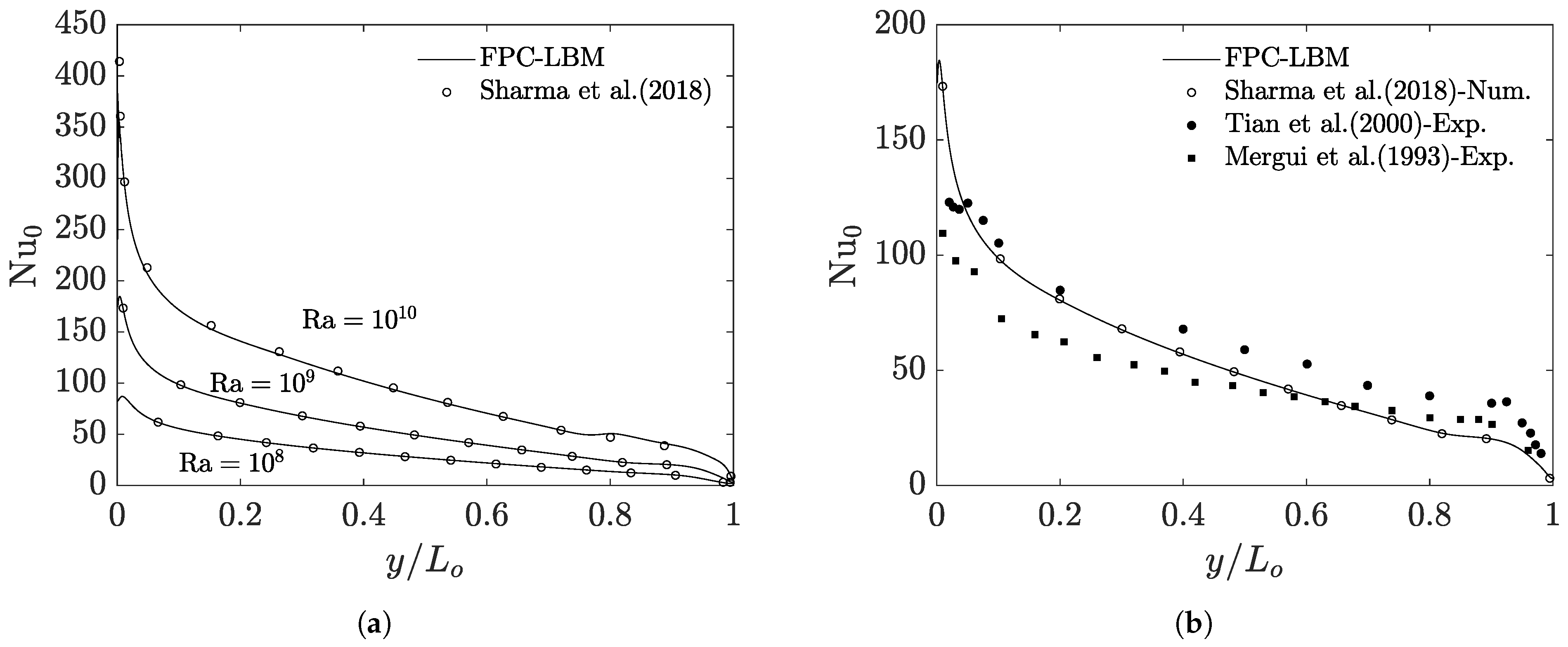
46], which we used for comparison.
Figure 7a shows the variation in the average Nusselt number along the hot wall from top to bottom for
,
, and
computed using the 2D FPC-LBMs and the results were time averaged over a duration of 90 million time steps. Shown in this figure are the prior numerical results of Ref. [
46] and our results are found to be in good quantitative agreement with it. Moreover, in
Figure 7b our results at
are also compared with the available experimental data of Refs. [
66,
67], which show satisfactory agreement given the measurement uncertainty inherent in the latter. In summary, these results indicate the FPC-LBM is a viable and accurate approach for thermal convective flows at high Rayleigh numbers.
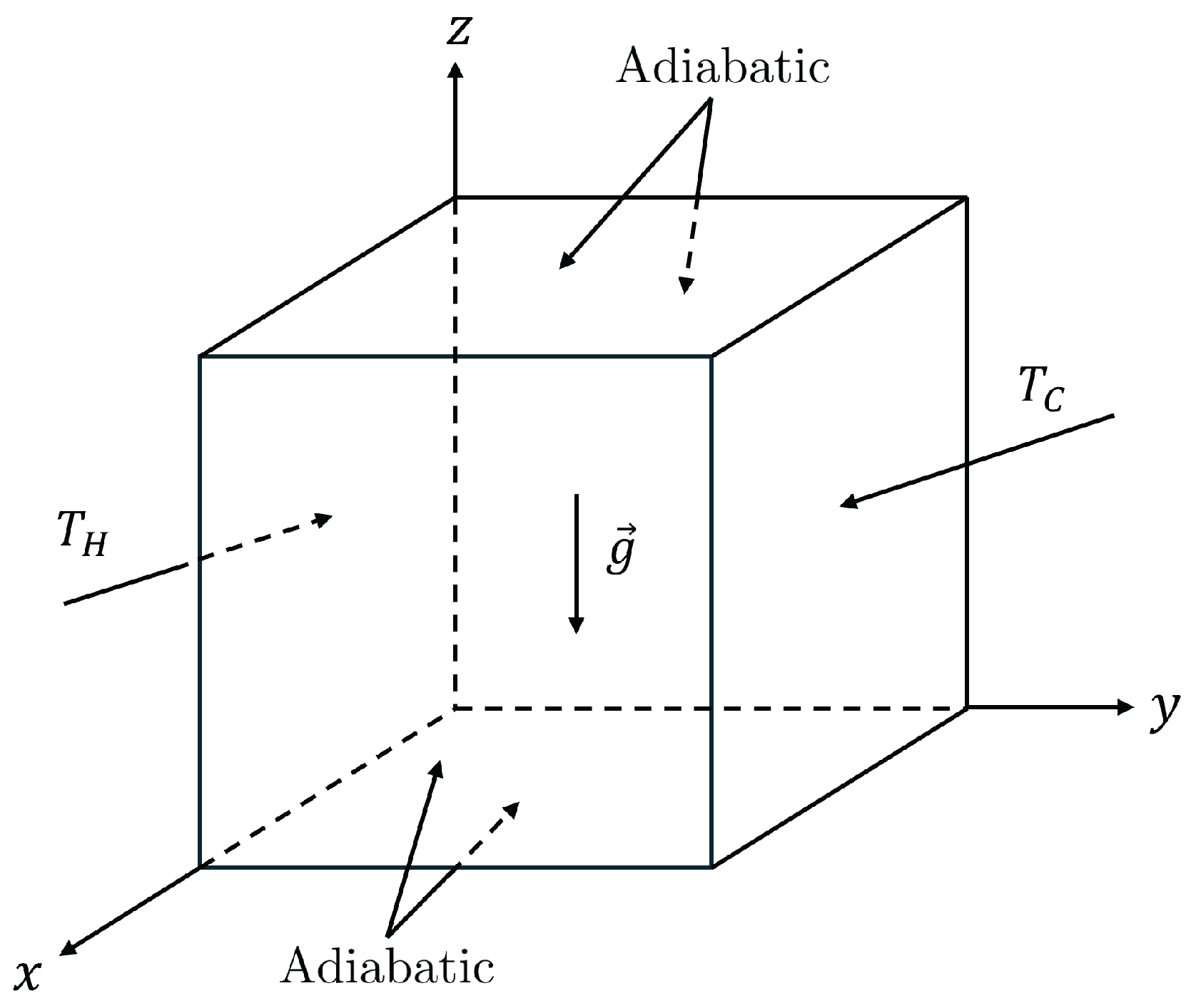
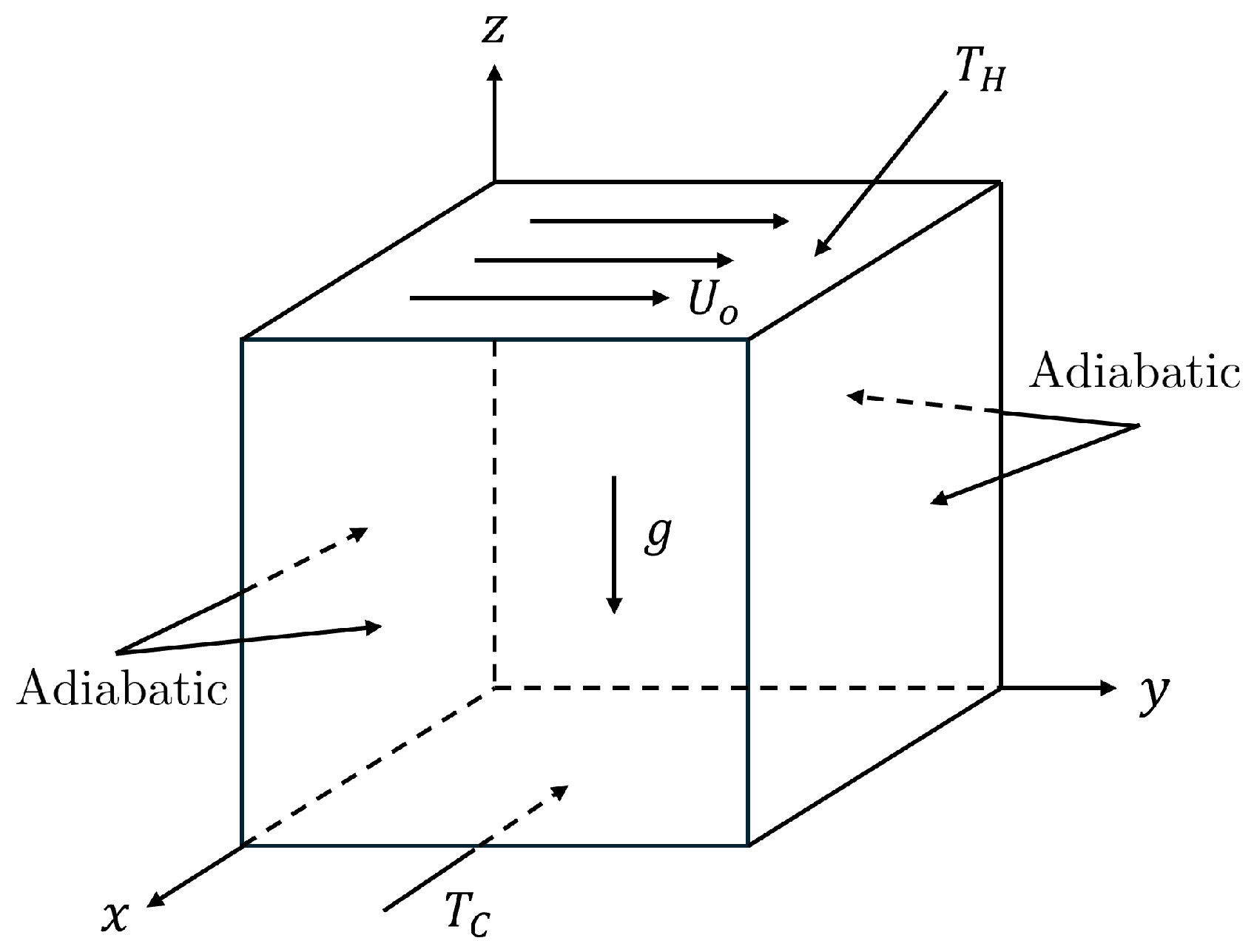
6.2. Natural Convection in a Cubic Cavity
Next, we discuss the simulation results of the natural convection inside a cubic cavity of volume
using the FPC-LBM on the D3Q27 lattice for hydrodynamics presented in our recent work [
33] and another FPC-LBM on the D3Q15 lattice for the energy equation discussed in
Appendix C. The no-slip boundary condition is applied on the velocity field on all wall surfaces; moreover, a constant and uniform hot temperature,
, is applied on the left side wall and a constant and uniform cold temperature,
, is applied to the right wall. All other walls are considered to be insulated and have zero temperature gradient in the normal direction as indicated in the schematic diagram in
Figure 8. The Boussinesq approximation is used to apply a buoyancy force
due to local changes in density that would otherwise occur due to local changes in temperature, resulting in natural convection; the local components of this body force are
,
, and
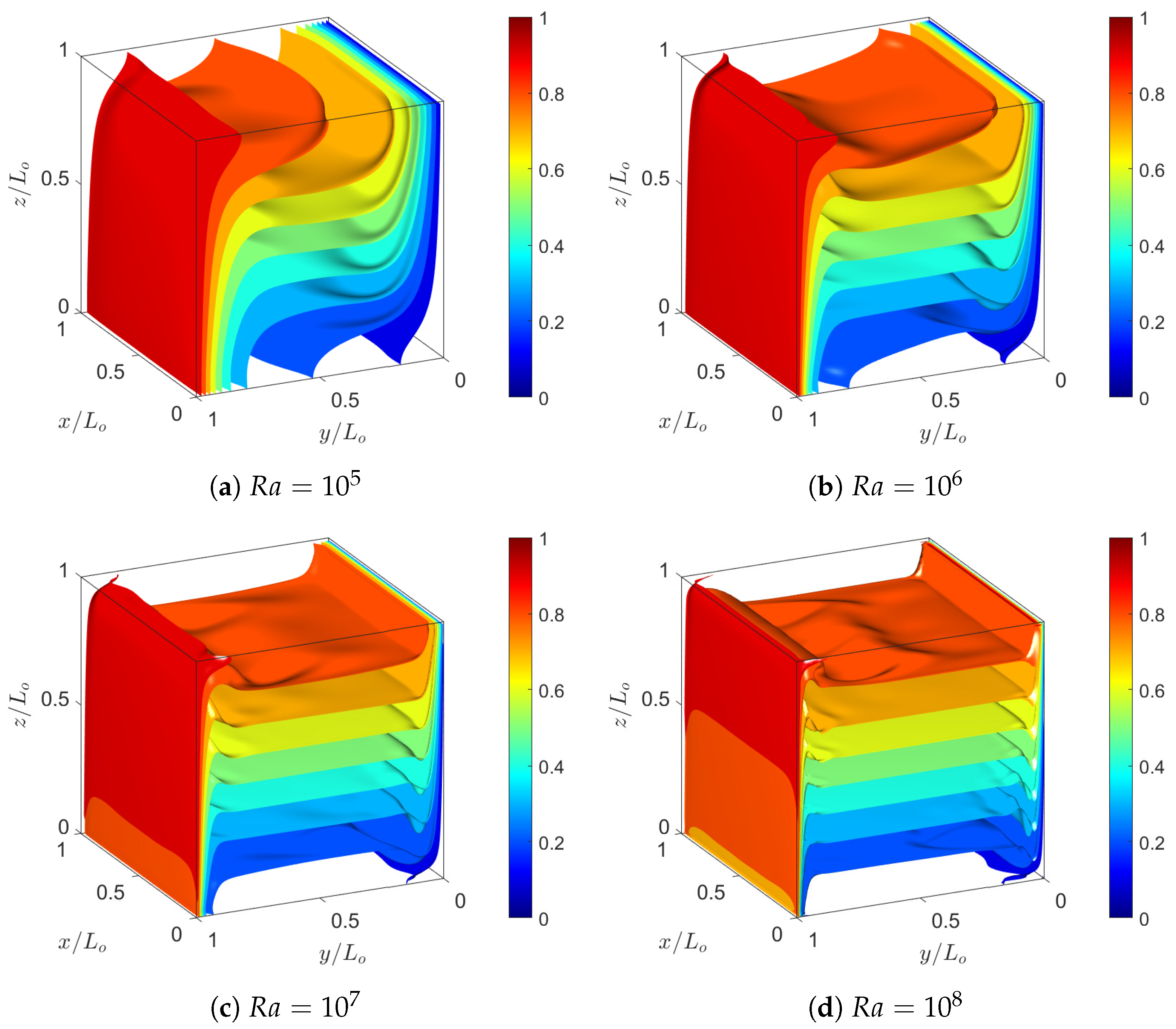
. In this work, we perform 3D simulations of natural convection in a cubic cavity at moderately high Rayleigh numbers.
Figure 9 shows the simulations results for
,
,
, and
indicating the isosurfaces of constant dimensionless temperature profiles between the values of
and
in increments of
, where
. They indicate that the formation of progressively thinner boundary layers near the walls with the imposed temperatures as the Rayleigh number is increased, and due to the presence of buoyancy forces they result in the vortex generation within the cavity. The natural convective flows thus formed cause an increase in the heat transfer rates as
is increased, which will be measured and evaluated in terms of the Nusselt number in what follows.
Before discussing further simulation results, we now provide an indication of the computational run times involved. The simulations were performed on the INCLINE parallel computer cluster hosted at the University of Colorado at Colorado Springs (UCCS). As an example, the turnaround time for performing
time steps of the simulation for the
case using
grid nodes on 512 cores was about
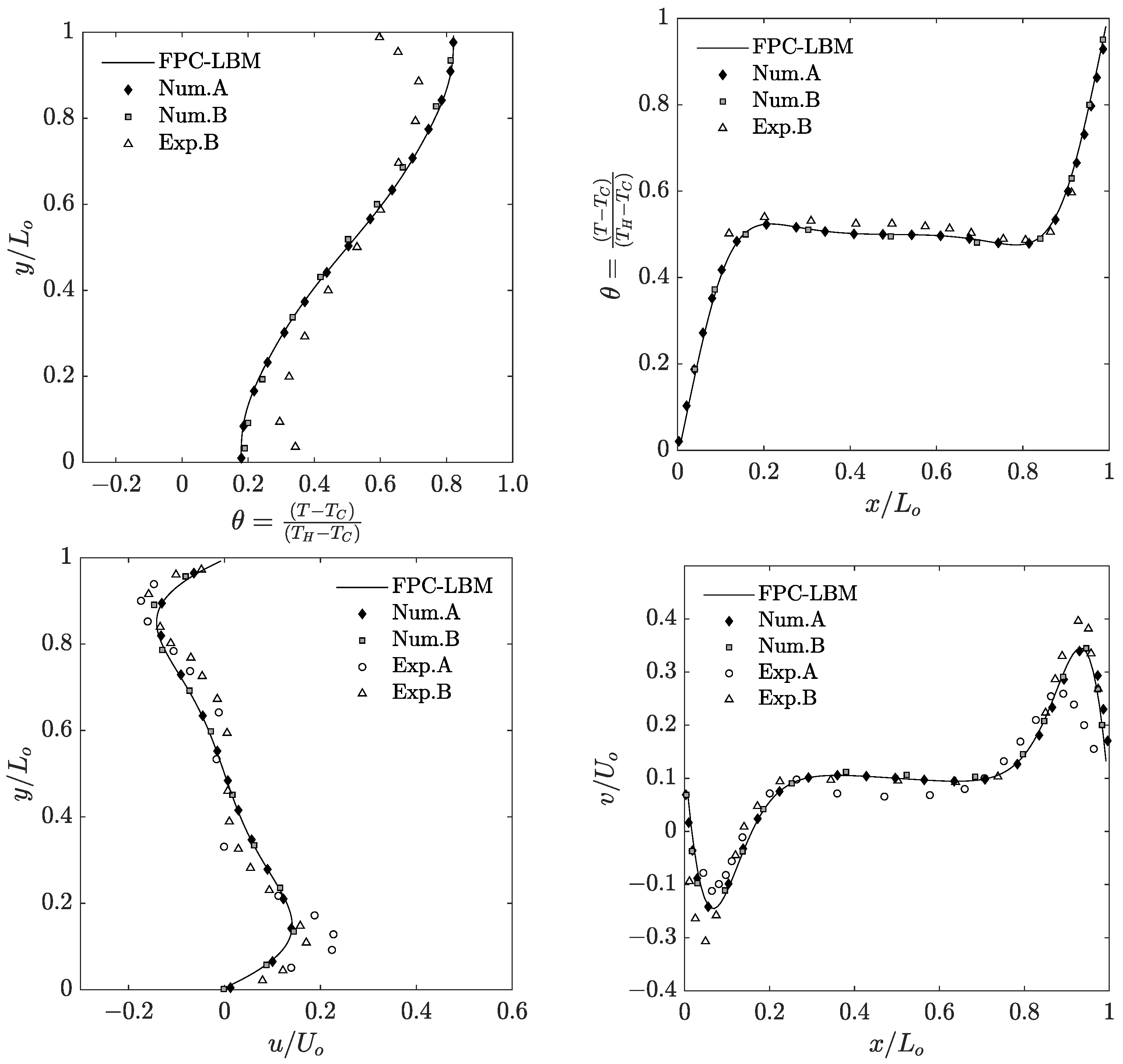
hours. Then, to obtain a quantitative comparison of the simulation results using the FPC-LBM, we look at the dimensionless temperature and natural convection velocity profiles along the vertical and horizontal centerlines in the primary mid-plane, and numerical [
64,
65] and experimental [
68,
69,
71] data available for the cases of
and
will be utilized as reference solutions in this regard. While such numerical solutions use the same velocity and thermal boundary conditions, it should be noted that the experimental data are subject to variations in the boundary conditions as the perfectly insulated condition is not always completely met; in particular, Krane (1983) [
68], Bilski et al. (1986), and Briggs and Jones (1985) [
71] consider thermally conducting top and bottom surfaces of the cavity in lieu of insulated boundaries. For example, this is illustrated by the experimental set up shown in
Figure 2 in Briggs and Jones (1985) [
71].
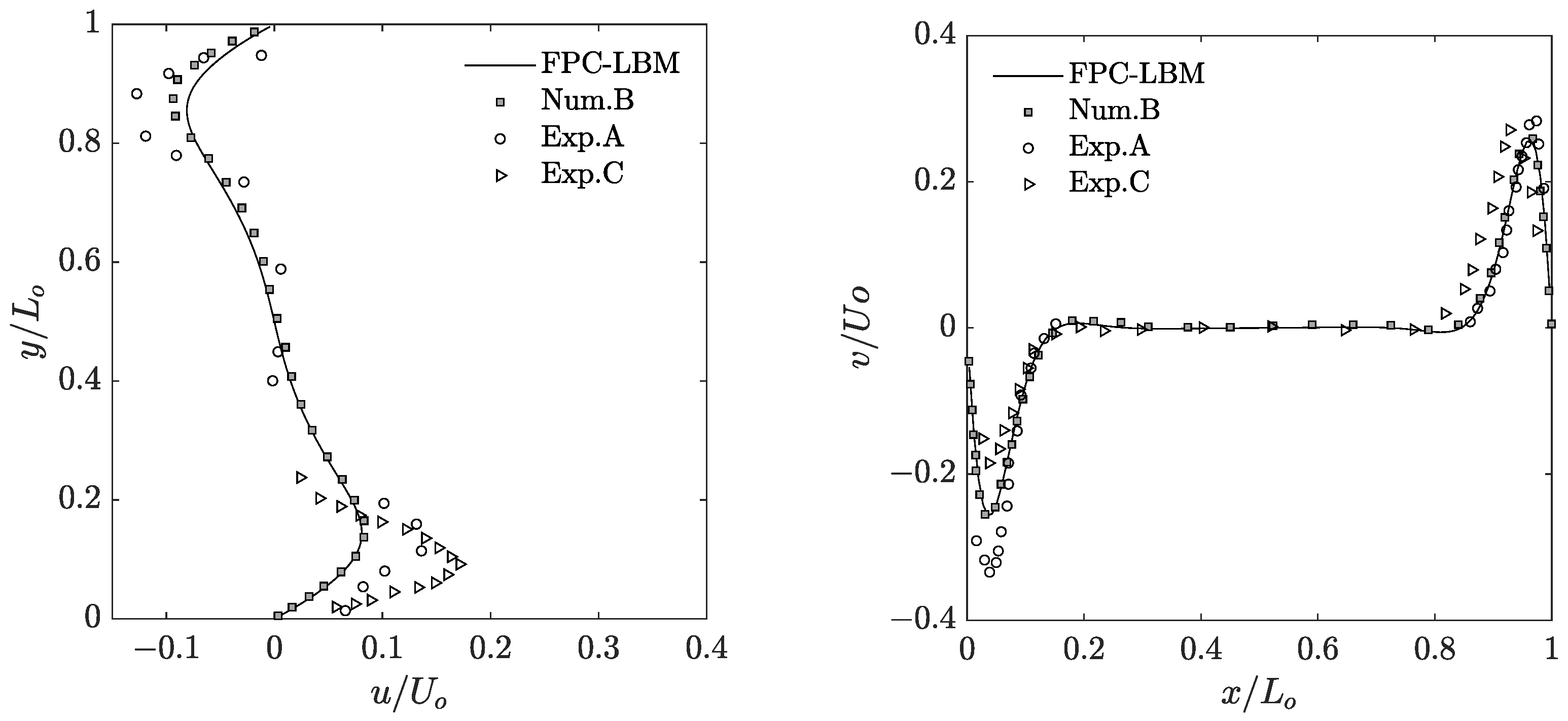
Figure 10 and
Figure 11 present the results and comparisons at
and
, respectively. While the FPC-LBM results are consistent with the experimental data across the domain associated with the constant wall temperature boundaries, some differences are noticed across the direction associated with the insulated boundaries, where, as noted above, the experimental set up does not have perfectly insulated surfaces, but conducting surfaces. Nevertheless, the FPC-LBM results are in very good agreement with the available numerical data for these cases.
Moreover, by quantifying the dimensionless heat transfer rates, we tabulate the average Nusselt number on the hot wall computed using the 3D FPC-LBMs and compare with prior numerical solutions available in the literature for
,
,
, and
in
Table 8. Our results are seen to be in very good agreement with these different sources of reference data.


