Abstract
Reasonable planning and scheduling in low-carbon parks is conducive to coordinating and optimizing energy resources, saving total system costs, and improving equipment utilization efficiency. In this paper, the optimization study of a distributed photovoltaic energy storage system considers the synergistic effects of the planning and operation phases. On the basis of the variable operating characteristics of the unit equipment and the complementary synergistic characteristics of the energy storage equipment, a two-layer optimization model combining planning and operation is adopted, with the minimum total cost and the minimum carbon emission content in the whole life cycle of the system as the optimization objectives and the upper layer of the planning equipment capacity and the configured capacity of each equipment in the system as the optimization variables, which are solved by using the multi-objective no-dominated-sorting genetic algorithm. The lower layer is the optimized operation mode, and the time-by-time operating capacity of each item of equipment is the optimization variable, which is solved by the interior point method. The upper layer optimization results are used as the constraint boundary conditions for optimization of the lower layer, and the lower layer optimization results provide feedback correction to the upper layer optimization results, which ultimately determine the energy system optimization scheme. The optimization results reflect that photovoltaic green power should be arranged in large quantities as a priority, and the synergistic effect of power and cold storage equipment on the system’s economy and low-carbon performance is positive. At the same time, by setting up four control scenarios of only cold storage, only electricity storage, no energy storage, and no two-tier optimization, the impacts of cold storage and electricity storage on the economic and environmental aspects of the system and the positive effect of mutual synergy are investigated, which concretely proves the validity of the two-tier optimization strategy, taking into account the operating characteristics of the equipment.
1. Introduction
Many countries around the world are actively promoting carbon emission reduction [1], with China striving to achieve carbon peaking around 2030 and carbon neutrality around 2060 [2,3], and the traditional energy model is shifting to a more flexible, diverse, and green distributed system [4]. Photovoltaic (PV) power generation is a clean energy source that plays an important role in balancing economic development and environmental protection. Compared with traditional energy sources such as coal and natural gas, PV power generation has the advantages of being renewable and non-polluting [5]. Compared with other renewable energy sources such as wind power and hydropower, PV systems are more suitable for installation in residential buildings [6]. A regional distributed photovoltaic system is a photovoltaic system installed in the vacant area of the building park, using local solar energy resources to achieve connection to the local grid and effectively reducing the energy loss associated with long-distance transmission with a small scale of investment, a short construction cycle, policy support, more flexible siting, and other advantages [7].
Currently, many regions in China lack electricity during peak tariff hours, which forces the government to take various power restriction measures during the peak of electricity consumption, resulting in buildings not being able to use electricity continuously. While there is more power generation, transmission, and distribution during valley tariff hours, they cannot be effectively utilized, and the use of peak and valley tariff differentials cannot be maximized and does not give full play to the significance of the implementation of peak and valley tariffs [8]. At the same time, due to the inherent characteristics of photovoltaic power generation, the generation of photovoltaic power in time with randomness and intermittency realizes the photovoltaic power generation system’s power output and regional energy demand in shorter time scales. There is a mismatch between the supply and demand sides of the imbalance between PV power generation, increasing the abandonment rate of photovoltaic power generation and resulting in the unstable operation of the power grid [9,10]. Therefore, in this case, there is an urgent need to study the planning and optimization methods of regional distributed systems and to establish a complete set of planning and optimization methods and systems to guide the construction and development of the region and realize the low-carbon transformation of buildings.
Bahramara used a hybrid optimization model for electricity and renewable energy (HOMER) developed by the National Renewable Energy Laboratory (NREL) for renewable energy system planning studies, which is widely used for renewable energy system equipment planning for loads ranging from 0.626 KW to 2213 MW [11]. Karunathilake et al. developed multiple scenarios for a park in Canada based on the cost of the whole life cycle and reductions in greenhouse gas emissions using scenario analysis to develop multiple scenarios for a park in Canada, evaluating the benefits of the scenarios and options [12]. The above studies focus on the design of energy sources and equipment in terms of type capacity, and distributed photovoltaic energy storage systems often need to consider both the planning results and the actual operation status. Jung et al. used the distributed DER-CAM model to design an equipment planning scenario and operation mode for a distributed microgrid system incorporating renewable energy sources [13]. Fujisawa et al. utilized the relationship between the variables in both the planning and operation phases to propose a model for the planning and operation of a distributed microgrid system [14]. Quashie et al. proposed a bi-level optimization model to solve the problem of the capacity planning of the equipment and operating power of the microgrid, with the objective of reducing the microgrid’s investment and operating costs [15]. Zhang et al. studied the planning and operation of an energy system in a building in Sweden, simulated the year-round operation of the building by setting up four different planning scenarios, and verified that the planning results could meet the operational requirements [16]. Yang et al. [17] designed a MILP model that can plan the location of energy stations, the capacity of the system’s equipment, the network layout of the entire system, and the system’s operational strategy model, which is currently operating in a region of Guangzhou City, China, proving that the optimized system has higher economic efficiency compared to the traditional system. Due to the contradiction between model accuracy and solution efficiency, the models studied above are simplified to a certain extent by setting the efficiency of the energy conversion equipment as a constant value in order to speed up the solution [18]. However, the efficiency of the energy conversion equipment is closely related to the load factor, while the temperature, air pressure, and other factors also impact it, and a constant value of efficiency will bias the calculation [19]. Through practical calculations, the authors of [20] observed that changes in the characteristics of un-equipped equipment at the design stage lead to a reduction in energy efficiency at design conditions, generating an additional expenditure of 11.57%. In addition, [21] used segmented linearization to approximate the variable operating condition efficiency curve method, which reduces the low computational cost but is greatly affected by the accuracy of the nonlinear equipment model and its part of the load rate under the equipment efficiency using a fixed value, which cannot accurately describe the actual efficiency of the equipment. The authors of [22] consider the characteristics of the variable operating conditions of equipment such as cogeneration units, gas boilers, absorption chillers, etc., in the optimized operation of integrated energy systems, but it is difficult to meet the operating standards of low-carbon parks due to the high carbon emissions of the system containing gas and other energy sources. The authors of [23] have segmented and linearized the characteristics of the nonlinear variable operating condition of the equipment and expressed the model as a mixed integer linear model. However, the same kind of equipment is regarded as a whole, and after considering the nonlinear variable operating condition characteristics of the equipment, it fails to reasonably allocate the output power of multiple pieces of the same kind of equipment. The operation of typical scenarios is closely related to the optimized configuration of distributed photovoltaics and energy storage. The diversity of scenarios directly affects the effectiveness of photovoltaic storage planning [24]. Zhao et al. [24] established an energy storage model for wind–solar complementary systems, optimizing the model for the maximum utilization rate of photovoltaic and wind energy and the minimum economic cost. However, the model lacks consideration of environmental impacts and does not focus on carbon emissions [25]. Li et al. developed a distributed power system for power sources, electric loads, and energy storage with a layered and partitioned control strategy for the distribution network. However, cooling systems, which also contribute significantly to energy consumption, are not clearly addressed [26]. Ding et al. built a distributed photovoltaic and energy storage system model with a combined heat pump and chiller for cooling. However, the model does not account for the variable operating conditions of the chiller units [27]. Liao et al. developed a two-level optimization model to address the allocation of distributed energy resources. The advantage of the model lies in its detailed simulation of risks on the grid side, but it does not consider the participation of cold storage devices [28].
In view of the above research on the regional energy system, this paper proposes a research method based on the bi-level optimization of a distributed photovoltaic energy storage park. The main contributions are as follows:
1. A bi-level optimization model based on a distributed PV energy storage system is proposed, which takes into account the variable operating characteristics of the unit’s equipment and the complementary synergistic characteristics of the energy storage equipment and plans the optimal capacity configuration of the equipment and the operating state of the typical day under the healthy operating state of each piece of equipment with the optimization objective of minimizing costs and carbon emissions;
2. By setting up four scenarios of distributed PV systems, namely no energy storage, cold storage, power storage, and cold storage combined with power storage, we study the influence of the presence or absence of energy storage and the complementary synergy of multiple energy storage devices on the planning and operation stage of the system;
3. By setting comparison scenarios comprising a distributed PV energy storage system with a bi-level optimization model and a distributed PV energy storage system with equipment capacity selected according to load and then system operation optimization, simulation calculations are performed for the two scenarios to verify the economy and low-carbon nature of the bi-level optimization model.
2. Systems and Operational Strategies for Low-Carbon Parks
2.1. System Description of Distributed PV Storage Systems
The PV distributed energy storage system in this paper is shown in Figure 1, which is mainly composed of PV modules, battery packs, the power grid, refrigeration units, ice storage tanks, and other equipment. For the regional power system, the battery controller is used to control the battery’s charging and discharging power, and the MPPT controller ensures the maximum output of PV power generation. The power generated by the PV modules can be supplied to the district’s consumers, the grid, and the battery bank through the DC/AC inverter. The power from the grid can be supplied directly to buildings or used to charge the batteries. For the district cooling system, a duplex refrigeration unit and a baseload chiller are involved in cooling, while an ice storage tank stores the excess cold and releases it when there is an insufficient supply of cold in the system and at times of peak electricity prices.
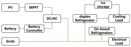
Figure 1.
Diagram of the distributed photovoltaic energy storage system.
2.2. Energy Dispatch Strategy
The cooling system of the park adopts the operation mode of a duplex refrigerator and an ice storage tank for ice storage and an on-board refrigerator for cooling. At night, when the electricity price is low, the duplex main engine is turned on to store ice, and the base load main engine is started to meet the lower cold load demand, which can shorten the time required to produce ice and ensure refrigeration efficiency. At other times, different cooling methods are used according to the electricity price:
1. Single ice-melting cooling supply: when the cooling load is small and the electricity price is unfavorable to the chiller’s cooling supply, the cooling load is completely satisfied by the cold volume generated by melting ice in the ice storage tank, which reduces operation costs.
2. Cooling supply using the main engine: when the electricity price is not at its peak or when the PV power is sufficient, the cooling load is provided by the main engine (including the on-board refrigerator and duplex refrigerator).
3. Joint supply using the ice storage tank and the chiller: during the daytime when the cooling load is large, the chiller and ice storage tank jointly supply cooling. During peak tariff hours, ice melting is mainly used to supply cooling, which is supplemented by chillers when the cooling load is insufficient. This operating mode optimizes electricity price utilization and reduces operating costs by reasonably scheduling different cooling methods.
For the park power system, battery charging and discharging can be flexibly controlled, improving the consumer’s initiative to manage the energy flow according to specific needs. In this study, an energy scheduling strategy with the goal of minimizing full-cycle economic operating costs and carbon emissions is used. The battery enters the storage state at night when the electricity price is low and the PV power is greater than the electrical load demand. If excess PV power still exists, it is exported to the grid. The battery enters the discharge state when the PV power cannot satisfy the load demand, and if there is still an energy gap, it will prioritize the import of power from the grid to cover the unsatisfied loads at moments when the electricity price is relatively low. Considering that frequent charging and discharging will affect the service life of the battery and that frequent switching of the state of the dual-condition chiller in the process of cooling and making ice will reduce efficiency, this study adopts a “one charge, one discharge” strategy, i.e., only one charging and discharging operation is carried out in each cycle, in order to reduce the burden on the equipment and improve the overall operational efficiency.
3. Bi-Level Optimization Model for Distributed PV Energy Storage Systems
3.1. Introduction to Optimization Frameworks and Strategies
In this paper, a multi-objective optimization framework for distributed photovoltaic (PV) energy storage systems in low-carbon parks is established. As shown in Figure 2, the optimization framework is divided into four parts, i.e., data preparation, planning optimization, operation optimization, and comprehensive evaluation. In this paper, data collection was first carried out to obtain load data, economic parameters, and technical parameters. Then, the planning model and operation model of the distributed PV energy storage system are constructed by adopting the optimization-seeking mode of bi-level optimization. Given the required parameters, the optimization model is solved using a comprehensive solution method to obtain the system’s equipment scheme and operating conditions. Finally, the results are comprehensively evaluated and comparatively analyzed.
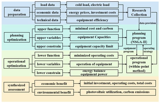
Figure 2.
Optimization framework for systems.
As shown in Figure 3, this paper adopts the strategy of determining electricity by cooling. First, according to the cold load, ice storage tank capacity, electricity price, etc., the ice storage tank’s operating state is optimized, and then the cold load is obtained after cold storage. According to the cold load after cold storage and the model and number of refrigeration units, the optimal operation of the refrigeration unit is calculated so as to obtain the optimized refrigeration power consumption. After formulating the optimization of the cooling system, according to the electric load, refrigeration power consumption, battery capacity, photovoltaic power generation, electricity price, and so on, the operating state of the battery is optimized, the electric load after storage is obtained, and the operating state of the power grid is calculated, completing the optimization of the electric system. Finally, the operation costs are calculated according to the operation status of each equipment and the energy utilization status. The full abbreviations used in this article are listed in Table 1.
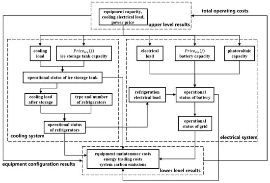
Figure 3.
Optimized scheduling strategy diagram for a typical day.

Table 1.
Definitions of acronyms and terms.
3.2. System Equipment Model
3.2.1. Refrigeration Unit Model
An electric refrigerator is a cooling unit in a distributed photovoltaic energy storage system. The efficiency of a refrigeration unit is not constant and is affected by its operating conditions or environment. It has been shown that the constant efficiency mode incurs an additional expenditure of 11.57% compared to the variable efficiency mode [20]. Usually, energy conversion devices need to consider the variable operating characteristics, as their inputs and outputs are not simply linear but vary with changes in load factor, temperature, air pressure, etc. [19]. Since the temperature, air pressure, etc., on the efficiency of the energy conversion equipment has a small impact, in order to simplify the analysis, it can be considered that there is some kind of functional relationship between the efficiency of the energy conversion equipment and its load factor. The relationship between the efficiency and load factor of multiple types of energy conversion equipment can be obtained by data fitting, and the generalized fitting formula can be expressed as follows:
where represents the cooling inlet temperature of the cooling unit at the current time, is the load factor of the refrigeration unit at the current moment, is the rated efficiency of the refrigeration unit, and is the actual efficiency of the refrigeration unit at the time t.
The model of the refrigeration unit’s cooling state is as follows:
where is the total cooling capacity of the refrigeration unit at time t, is the electrical power used for cooling by the i refrigerator, is the conversion efficiency of equipment cooled by the i refrigerator, and is the actual efficiency of the i refrigerator at time t.
The process of making ice involves transferring heat from water or a liquid to the environment and cooling it to a temperature sufficient to form ice. This requires more heat transfer, and during the ice-making process, the liquid needs to overcome the heat of phase change to transform into a solid state, which means that more energy is required to bring the liquid to its freezing point and form ice; therefore, the COP will be lower during ice-making than in refrigeration.
The model of the refrigeration unit’s ice production state is as follows:
where is the total ice output from double-condition refrigeration, is the electrical power of i double-condition refrigeration for ice production, is the conversion efficiency for ice production in i double-condition refrigeration, and is the correction factor for ice production in double-condition refrigeration.
3.2.2. Ice Storage Tank Model
3.2.3. Battery Model
The model of the battery’s charge state is as follows:
where the battery charge state at time t, is the remaining capacity of the battery at time t, and is the total capacity of the battery.
The battery charging and discharging model is as follows:
where is the battery charge state at time t − 1, is the energy storage loss rate of the battery, is the battery charge at time t, is the battery discharge at time t, is the battery charging power loss rate, and is the discharging power loss rate.
3.2.4. Photovoltaic Model
Photovoltaic power generation is issued by the size of the power and the surrounding ambient temperature, the intensity of solar radiation, and the size of the assigned rated power. The output power calculation model is as follows:
where is the actual power output from PV, is the rated output power of PV under standard conditions, is the surface temperature of PV power generation under standard conditions, with a size of 25 °C, is the surface temperature of PV power generation in real conditions, k is the temperature coefficient of PV power generation for power output, taking , is the light intensity required for photovoltaic power generation under standard conditions, and is taken as , and is the intensity of light received by PV power generation under actual conditions.
Since it is not easy to measure the surface temperature of the PV panels during the actual operation of the project, it can generally be estimated based on empirical formulas:
is the actual ambient temperature.
3.3. Bi-Level Optimization Objective Function and Constraints
The optimization objective in the upper-level planning optimization model is to minimize the cost and carbon emissions over the whole life cycle of the energy system, while lower-level operation optimization is an operation optimization simulation based on the configured capacity of upper-level planning, and the decision variables are the hour-by-hour operation quantities of each major piece of equipment in the system, which need to satisfy the operation limitation constraints and energy balance constraints of the equipment.
3.3.1. Upper-Level Device Constraints
3.3.2. Upper-Level Objective Function
DTC (daily total cost):
is the initial investment cost. The initial investment cost of a distributed PV energy storage system is mainly the purchase cost of the equipment in the system. Meanwhile, based on the service life of the system, the investment cost is converted into a typical daily average cost, which can be expressed as:
where is the recovery coefficient for the equipment, is the discount rate of the equipment, is the useful life of the equipment, is the number of equipment, is the rated capacity of equipment , and is the price per unit capacity of the equipment.
where represents equipment installation and transportation costs, and is the investment proportion coefficient of the installation cost.
where is the operation and maintenance costs of the equipment, is the unit cost of equipment i, is the total energy produced on a typical day for equipment i, and is the energy consumption costs.
where is the grid electricity price at time t, are the amounts of power purchased and sold by the grid at time t, respectively, and is the grid electricity price for surplus electricity from photovoltaic power generation, taking the benchmark electricity price for desulfurization as 0.3598.
TCF (total carbon footprint):
where is the indirect carbon emission factor from grid power purchases, with a specific carbon emission factor value of .
3.3.3. Lower-Level Goal Constraints
Battery Constraints
Electric load transfer volume constraint: transfer volume < load:
Battery capacity constraints: sum of charges on a typical day < maximum battery capacity:
Battery SOC constraints:
Equal state of charge at the beginning and end of battery storage:
SOC ranges from 0 to 1. indicates that the battery is fully discharged, while indicates that the battery is fully charged. Deep charging and discharging of the battery will reduce its service life; therefore, usually has a limit:
where are the maximum and minimum values of the charging state of the battery, respectively. takes 0.1, takes 0.9.
Battery charging and discharging power constraints: the charging and discharging capacity of the battery at time t is less than or equal to the maximum value of the charging and discharging capacity of the battery per unit hour:
Refrigeration Unit Constraints
The hourly cooling capacity of the chiller is between 0 and the maximum hourly cooling capacity:
Cold Storage Tank Constraints
Energy storage state constraints for the accumulator tank are as follows:
Ice storage and melt rate constraints for cold storage tanks are as follows:
PV System Constraints
PV power generation at moment t is greater than or equal to 0:
Grid Constraints
Purchased power from the grid is less than or equal to the maximum amount of purchased power:
Energy Balance Constraints
Cold system equilibrium constraints are as follows:
Electric system equilibrium constraints are as follows:
is the required cooling load at moment t and is the required electrical load at moment t.
3.3.4. Lower-Level Objective Function
Considering the grid price difference of the battery’s charging and discharging efficiency, for the same part of the charging energy, there will be energy loss when it is discharged. Considering the peak and valley tariff arbitrage generated by this part of the charging energy, the battery charging quantity can be analyzed from another angle as part of the load transfer from the moment of to the moment of . The energy loss is taken into account in the tariff difference, so it can be considered that this part of the power ‘does not exist’ in terms of power loss, that is, how much power can be discharged by charging how much power.
Similarly, according to the equipment, the conversion rate can be obtained:
The total economic cost of the system is minimized by and the profit maximization function is maximized by using the peak-to-valley difference in electricity prices by as follows:
where is the amount of load transfer from the moment of high electricity prices to the moment of low electricity prices under the j type of electricity price differences, is the grid price difference considering battery charging and discharging efficiencies under j tariff difference, is the ice-melting volume of the ice storage tank under j tariff type, is the grid price difference considering the ice storage efficiency of the ice storage tank under the j type of tariff difference, is the ice storage tank’s capacity, is the number of battery cycles, is the number of ice storage tank cycles, is the initial investment per unit of battery capacity, and is the initial investment per unit of ice storage tank capacity.
4. Solution Methods
4.1. Introduction to the Algorithm
The multi-strategy gravity search algorithm (GSA), particle swarm optimization algorithm (PSO), ant colony optimization algorithm (ACO), simulated annealing algorithm (SA), etc., have been widely used to solve regional planning problems. Table 2 shows the advantages and disadvantages of each algorithm, and it is found by comparison that the genetic algorithm has better global search capability than other solution algorithms in multi-objective operation optimization. In addition, its selection, crossover, and mutation operators effectively avoid the local minimum trap that other optimization algorithms may encounter. Genetic algorithms have good convergence, and the shorter computation time has a certain robustness; however, in practice, genetic algorithms are prone to the problem of premature convergence at a later stage. Therefore, this paper adopts a fast non-dominated individual sorting method based on the congestion distance operator of the genetic algorithm to maintain the diversity of the population in order to obtain the Pareto solution set for the planning and operation of distributed photovoltaic energy storage systems. Linear programming algorithms are mature and efficient and have been widely used to solve a variety of practical engineering problems, such as energy system operation scheduling problems, etc. In this paper, the interior point method is used instead of the traditional linear programming method, which has a faster convergence speed, wider applicability, and is able to deal with non-smooth problems, which effectively improves the flexibility of the optimal scheduling. The TOPSIS method has the advantages of a robust logical structure, a simple computational process, and the ability to consider both ideal and negative solutions. In this paper, the TOPSIS comprehensive evaluation decision model is used to evaluate and analyze the Pareto solution set to obtain the final optimal solution.
Table 2.
Comparison of algorithms.
4.2. Bi-Level Optimization Model Solution Structure
In this paper, a bi-level optimization model linking operation and planning is constructed to simulate and feedback the optimization of the planning equipment capacity with the equipment operation condition, and the flow chart of its solution structure is shown in Figure 4. The upper-layer optimization is the optimization of the planning equipment capacity, taking the minimum average cost of the whole life cycle and the environmental cost of carbon emissions as the optimization objective. The optimization variable is the configured capacity of each piece of equipment in the system, which is optimized using the NSGA-II algorithm under the condition of satisfying the equipment capacity constraints. The lower-level optimization is the operation optimization, with the objective of minimizing the operation costs. The optimization variables are the operation status and output of each piece of equipment, and the operation status of the equipment is obtained by using the interior point method planning under the condition of satisfying the operation constraints of each piece of equipment. The relationship between the upper and lower layers of optimization is that the results of the upper layer of planning optimization are used as the upper constraints of the variables of the lower layer of operational optimization, and the results of the lower layer of operational optimization provide feedback corrections to the results of the upper layer of planning optimization to finally obtain a Pareto solution set that satisfies the matching of the operation. Finally, the Pareto solution set is evaluated and analyzed using the TOPSIS comprehensive evaluation and decision-making model to obtain the final optimal solution.
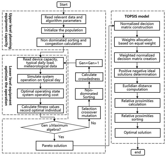
Figure 4.
Process of the model-solving algorithm.
5. Analysis of Examples
This paper uses a zero-carbon district in Beijing, China as a case study. The district includes a hotel building of 2160 m2, a shopping mall of 4227 m2, an office building of 4385 m2, and a residential building of 1347 m2. The summer high-temperature period is the peak time for annual energy consumption and also the season with the greatest energy fluctuations in the system. If the system’s planning and operational strategies are not properly designed, it could lead to energy supply shortages or even energy shortages. Therefore, this paper focuses on optimizing the design and operation of the district for the entire cooling season, establishing a configuration plan for the equipment within the district and the hourly operation status of the equipment on a typical sunny day in the summer. The results indicated that the average calculation time for a single optimization run is within the acceptable range for practical energy system planning. The specific programmers are as follows:
1. Establish a distributed photovoltaic system that integrates cooling and energy storage. This scenario serves as the baseline for comparison with subsequent scenarios, validating the economic and low-carbon performance of the distributed photovoltaic energy storage system proposed in this paper;
2. Set up distributed photovoltaic systems that only include cooling storage, only include energy storage, and exclude energy storage. By comparing these systems with each other and the baseline scenario, this analysis explores the varying impacts of cooling and energy storage modes on the district’s economy, environment, design, and operation, as well as the benefits generated by the synergistic effects of the two energy storage modes on the district system;
3. Establish a distributed photovoltaic system under the traditional planning model without dual optimization. This will validate the economic and low-carbon performance of the distributed photovoltaic energy storage system with the dual-optimization model proposed in this paper by comparing it with the baseline scenario.
5.1. Data Parameters
The district includes four types of buildings: hotels, shopping malls, offices, and residences. The design of the district follows the enclosure standards specified in the “GB/T 51350-2019 Technical Standard for Nearly Zero Energy Buildings” [29]. Table 3 presents the heat transfer coefficients of the building envelope and the Solar Heat Gain Coefficient (SHGC) standards for public and residential buildings in Beijing.
Table 3.
Heat transfer coefficients of low-carbon building envelopes and SHGC.
The hotel building in the district has an area of 2160 m2, a ceiling height of 3 m, and a total of three floors, with each floor having an identical area. The model includes offices, corridors, guest rooms, equipment rooms, and other spaces. The shopping mall building has an area of 4227 m2, with 3272 m2 of air-conditioned space, a ceiling height of 5.7 m, and two floors. The first floor has a total area of 2170 m2, and the second floor has a total area of 2057 m2. The model includes a Chinese restaurant, a Western restaurant, corridors, restrooms, equipment rooms, and other spaces. The office building has an area of 4385 m2, with 3127 m2 of air-conditioned space, a ceiling height of 4.5 m, and a total of three floors. The first floor has a total area of 1573 m2, the second floor has an area of 1501 m2, and the third floor has an area of 1311 m2. The model includes lounges, offices, corridors, meeting rooms, storage rooms, and other spaces. The residential building has an area of 1347 m2, with 1092 m2 of air-conditioned space, a ceiling height of 2.85 m, and a total of three floors, with each floor having an identical area. The model includes restrooms, a kitchen, a master bedroom, a secondary bedroom, a study, a living room, and other spaces. According to the policy standards of Beijing, this paper selects the period from 15 May to 15 September as the cooling season for the entire year. The hourly cooling load and hourly electrical load data for the entire cooling season of the district are shown in Figure 5.
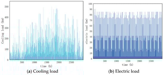
Figure 5.
Load during the cooling period in the park.
It was observed that the cooling load fluctuates significantly throughout the cooling season, while the electrical load exhibits similar daily fluctuations. To verify whether the equipment configuration can fully meet the energy supply and scheduling requirements of the district’s system, the typical operational day for this chapter is selected as the day corresponding to the peak cooling load during the entire cooling season, specifically July 10th, which is chosen as the typical day for this study. The 24 h cooling load and 24 h electrical load data for the typical day of the district are shown in Figure 6. It is important to note that the electrical load mentioned here excludes the portion of electrical energy consumption caused by cooling. Since the selection of different refrigeration compressor units and the operating conditions of ice storage tanks can affect refrigeration electricity consumption, it is necessary to first determine the optimal cooling system configuration in order to obtain more accurate refrigeration energy consumption. This allows for the calculation of the district’s electrical load after considering cooling, which corresponds to the “cooling-based electricity” operational strategy mentioned earlier.
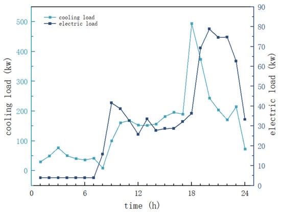
Figure 6.
Typical daily cooling load and electrical load in the park.
The cooling load in the district is relatively low between 00:00 and 08:00, as only the hotel and residential buildings are in operation during the nighttime and early morning hours. As office workers arrive and the shopping mall begins to operate, the cooling load gradually increases between 08:00 and 10:00. From 10:00 to 17:00, the cooling load stabilizes with small fluctuations. Between 17:00 and 18:00, due to the shopping mall entering its peak hours and the office buildings still in operation, the cooling load reaches its daily peak. From 18:00 to 21:00, as the office buildings stop operating at 18:00 and the shopping mall stops at 21:00, the cooling load begins to decrease. Between 21:00 and 24:00, as indoor activities in the residential and hotel buildings decrease, the overall cooling load in the district also decreases. Similarly, the electrical load is low between 00:00 and 07:00, then rapidly increases between 07:00 and 09:00, for the same reasons as the cooling load fluctuations. From 09:00 to 12:00, the electrical load decreases slightly due to the outflow of people from the hotel and residential buildings. Between 12:00 and 18:00, the electrical load fluctuates slightly but stabilizes. From 18:00 to 20:00, the significant electricity usage during the shopping mall’s peak hours causes the district’s electrical load to rise sharply. From 20:00 to 24:00, as the shopping mall stops operating and indoor activity in the residential and hotel buildings decreases, the overall electrical load in the district gradually decreases. Based on the analysis of the cooling and electrical load fluctuations on this typical day, the fluctuations align with the behavioral patterns of the district’s occupants and the operational conditions of the buildings. At the same time, the unit area load indicators for each building in the district comply with low-carbon standards, and the accuracy of the load data has been validated.
The electricity price information from the “State Grid Beijing Electric Power Company’s Proxy Purchasing Electricity Price Table for Commercial and Industrial Users” is used. This pricing adopts a time-of-use tariff system, which is divided into four categories: peak, flat, valley, and off-peak prices, with different rates set according to electricity demand at different times. Through this mechanism, peak electricity demand can be effectively managed, avoiding resource waste and cost increases. The specific electricity prices are shown in Figure 7a. Outdoor temperatures can affect the operating conditions of the equipment. The cooling unit model used above is related to outdoor temperatures in terms of its operational efficiency. Solar radiation intensity is one of the most important factors influencing the electricity generation efficiency of photovoltaic equipment. Figure 7b,c depict the hourly outdoor temperature and photovoltaic power generation per unit area on a typical day.
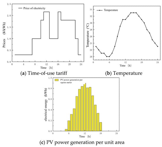
Figure 7.
Electricity price information and meteorological parameters.
The operating cost and technical parameters of the equipment are important factors influencing the optimization objective and directly determine the operation strategy of the equipment. The cooling unit selected is a dual-condition cooling unit. Based on market research, a cooling unit from a company in Jiangsu Province, China was chosen to determine the unit cost per capacity. The photovoltaic module selected is a photovoltaic panel, with the construction price per square meter determined based on the national conditions for photovoltaic installations in China. Lithium batteries are chosen for energy storage, and the prices for ice storage tanks and batteries are also determined based on market research to establish the unit cost per capacity. The specific economic parameters of each device are shown in Table 4.
Table 4.
Economic parameters of the main items of equipment.
The setting of algorithm parameters affects the optimization calculation’s speed and accuracy. It is necessary to specify the basic parameters for the upper-level genetic algorithm (NSGA-II) and the lower-level interior-point method in the bi-level optimization model, including the population size, number of iterations, crossover probability, optimal overall parameters, maximum function evaluations, and maximum iteration counts. Additionally, before running the model, the upper and lower limits of various constraints must be specified, i.e., a reasonable search range, in order to save computation time and achieve the optimal solution. Table 5 shows the results of the algorithm parameter settings and the constraints on the equipment search range.
Table 5.
NSGA-II algorithm parameter setting.
After the bi-level optimization calculation and analysis, Table 6 presents the equipment configuration schemes for each scenario. The five scenarios are as follows: 1. Bi-level optimization example of a distributed photovoltaic energy storage system with cold storage and electricity storage coordination. 2. Bi-level optimization example of a distributed photovoltaic energy storage system with only a cold storage mode. 3. Bi-level optimization example of a distributed photovoltaic energy storage system with only an electricity storage mode. 4. Bi-level optimization example of a distributed photovoltaic system without energy storage. 5. Traditional optimization method example of a distributed photovoltaic energy storage system with cold storage and electricity storage coordination. A detailed results analysis of each scenario follows.
Table 6.
Equipment planning schemes for each scenario.
5.2. Scenario 1: PV Distributed System with Cooperative Cooling and Power Storage
Scenario 1 is the baseline scenario for the entire example, setting a distributed photovoltaic energy storage system that includes both cold storage and electricity storage devices. From Table 5, it can be seen that the photovoltaic area is 2010 m2, and its total electricity generation fully covers the total electricity demand of the park, achieving zero carbon emissions. Subsequent operation results will demonstrate this. Photovoltaics are clean and renewable energy sources that reduce carbon emissions. At the same time, photovoltaic power generation can reduce the amount of electricity purchased from the grid, lowering the operating costs of the distributed photovoltaic energy storage system and offering high economic benefits. The cooling unit selects a two-large-one-small configuration scheme. This configuration allows the cooling equipment to operate at high efficiency for most of the working time, and the subsequent operation results will demonstrate this. The use of batteries can fully take advantage of time-of-use electricity pricing, significantly reducing system operating costs and carbon emissions. The capacity of the ice storage tank is larger than that of the battery because its investment and maintenance costs are much lower than those of the battery. However, the cold storage capacity of the ice tank is smaller in terms of the system’s overall scheduling capability compared to the battery, requiring a larger capacity to perform its full scheduling function.
Since this system uses the logic of cooling-based electricity determination, it is necessary to first analyze the cooling system of the park. The operational status of the cooling system under the optimal configuration is shown in Figure 8a. From t = 7 to t = 15, due to high solar radiation, the system’s photovoltaic generation far exceeds the total electricity demand of the park. There is an urgent need to absorb the photovoltaic power. A dual-condition cooling unit is activated to start ice-making and store the ice in the ice storage tank for use during electricity shortages, while other cooling units meet the current cooling load demand. From t = 0 to t = 4 and t = 19 to t = 24, the system uses ice storage tank cooling as the main cooling method. This is because there is no photovoltaic power generation at night, and the cold energy stored during the day needs to be released to reduce the cooling load, thus lowering the refrigeration electrical load and reducing the park’s electricity load at night, compensating for the insufficient renewable energy supply. At t = 5 and t = 6, a single cooling unit is used to supply cooling. The small cooling load can be met by activating the smallest cooling unit. At t = 16, a single cooling unit is used again, but a larger cooling unit is activated to meet the park’s cooling demand. At t = 17 and t = 18, a combined cooling mode with a single large cooling unit and the ice storage tank is used to reduce the refrigeration electrical load as much as possible while also meeting the cooling demand.
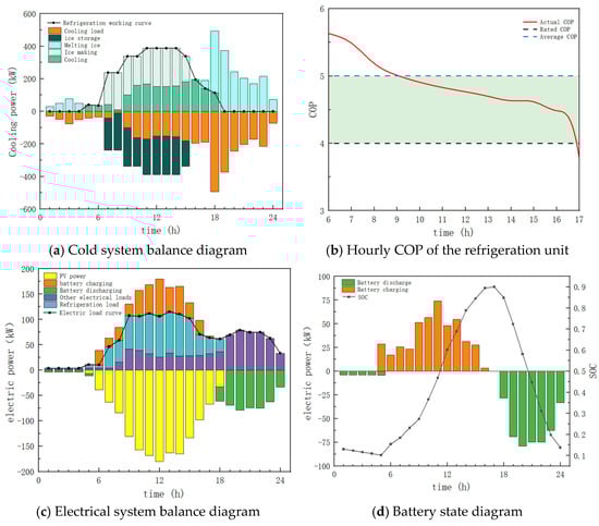
Figure 8.
Optimization results of Scenario 1.
Figure 8b shows the hourly COP of the cooling unit under a typical daily operation mode. From the figure, it can be seen that the actual COP of the cooling unit remains higher than its rated COP, with an average COP of 5.03, validating the effectiveness of the cooling system optimization. The reasonable optimization of the cooling system improved the operational efficiency of the cooling unit. Reducing the refrigeration electrical load indirectly lowered the park’s carbon emissions and reduced electricity-related economic costs for the park.
Figure 8c illustrates the operational state of the campus electrical system on a typical day. Observing the data above the y = 0 axis, after adding the cooling electrical load, the electrical load curve of the campus shows low values between t = 0 and t = 5. From t = 6 to t = 9, the electrical load continuously increases and approaches its peak value. Between t = 9 and t = 15, the load fluctuates near the peak value. From t = 15 to t = 18, the load gradually decreases, and between t = 18 and t = 23, the electrical load fluctuates within a range of 50–65% of the peak value. By t = 24, it decreases to below 40% of the peak value. It can be observed that after optimizing the cooling system, by adjusting the cooling electrical load, the total electrical load of the campus exhibits two smooth peaks, and the overall load curve becomes flatter. This significantly reduces the difficulty of energy scheduling in the electrical system. Further analysis in Scenario 3 will demonstrate the positive impact of the thermal energy storage system on the campus. Observing the data below the y = 0 axis, the photovoltaic panels start generating electricity at t = 5, reaching their peak generation at t = 12, which then begins to decrease. After t = 18, the photovoltaic panels no longer generate electricity. It can be observed that the entire electrical load of the campus is supported by photovoltaic power generation and battery discharging, with no need to purchase electricity from the grid. This allows the campus to achieve energy self-sufficiency and reach the ultimate goal of zero carbon emissions.
The typical daily charge and discharge state of the battery and its SOC are shown in Figure 8. Throughout the entire cooling season, t = 17 (when the battery SOC is at its maximum) is considered the end of each day. The battery operates in a charge–discharge cycle within each 24 h period, charging from t = 6 to t = 17 and discharging from t = 18 to t = 5 the following day. Additionally, throughout the day, the battery’s SOC remains within the range of 0.1 to 0.9, ensuring the battery’s health and stability while also meeting the maximum charge and discharge power limits. This confirms the rationality of the research method in the planning and operation of energy storage devices within the campus system.
After calculation, the operating cost for the entire cooling season in this scenario is CNY 84,147. When considering the initial purchase cost of the equipment, the total cost for the cooling season is CNY 170,467. The operating cost for the typical day on July 10 is CNY 715, with the total daily cost (including the initial purchase cost) being CNY 1441. Under the operating mode of Scenario 1, the carbon emissions for the entire cooling season on the campus are zero. The photovoltaic consumption rate for the whole campus reaches 98.37%, with the typical day achieving a photovoltaic consumption rate of 100%, thus realizing zero carbon emissions for the campus.
5.3. Scenario 2: PV Distributed System Containing Only Cooling Storage
Scenario 2 serves as a comparison scenario for the example. It is designed with a distributed photovoltaic energy storage system that only includes thermal storage equipment. The equipment design, planning, and operational scheduling for the entire cooling season of the campus are based on this configuration. The optimized equipment capacity configuration results are shown in Table 5. From the table, it can be seen that the photovoltaic area is 1452 m2, covering 72.45% of the campus’s electricity demand, thus meeting the technical requirements for a nearly zero-energy campus. The capacity of the ice storage tank is 2338 kWh, which can fully support the cold load supply during periods when the campus’s renewable energy generation is insufficient. The cooling unit selection includes one 120 kW unit and two 190 kW units. This configuration allows the cooling units to maintain high efficiency under normal operating conditions.
The following section will further verify the configuration results through the typical day’s operational scheduling.
The operational state of the cooling system under the optimal configuration is shown in Figure 9a. During the nighttime periods with no photovoltaic generation, from t = 0 to t = 4 and from t = 19 to t = 24, the entire cooling load of the system is handled by the ice storage tank. At t = 5, the ice storage cooling mode is adopted due to the small cooling load. At this time, the chiller is turned on, but due to the low load, it can only operate at a lower efficiency. Since the ice storage tank has sufficient capacity, the chiller does not operate and cooling is provided by the ice storage tank. At t = 18, the ice storage cooling mode is adopted because, although there is photovoltaic generation in the system, the campus’s electrical load is at its peak. The photovoltaic power is prioritized for other electrical loads and cannot meet the cooling load demand. Thus, the cooling load is handled by the ice storage tank, alleviating the campus’s power supply pressure. From t = 6 to t = 15, the photovoltaic generation is much greater than the total electrical load of the campus, creating a need to absorb the excess photovoltaic power. One small dual-mode chiller and one large dual-mode chiller are turned on to start ice production, which is stored in the ice storage tank for use during times of electrical shortage. Meanwhile, another large chiller meets the current cooling load demand. At t = 16, the ice storage tank reaches its energy storage limit, and only one large chiller is turned on to meet the cooling load demand. At t = 17, both the small chiller and the ice storage tank are used simultaneously to meet the cooling load demand, reducing the cooling electrical load and alleviating the campus’s power supply pressure.
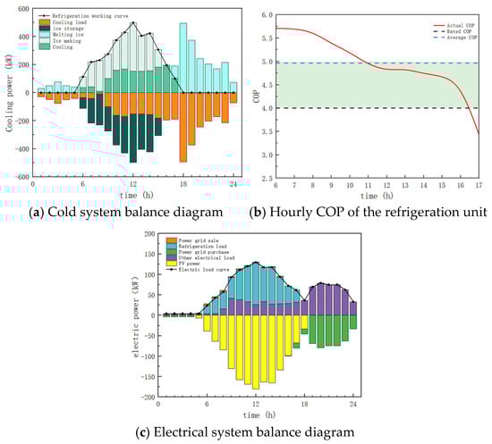
Figure 9.
Optimization results of Scenario 2.
Figure 9b presents the hourly COP of the chiller unit under the typical day’s operating mode in Scenario 2. From the figure, it can be seen that the chiller unit operates only during the daytime, and its actual COP is higher than the rated COP most of the time. The average COP reached 4.95, which validates the effectiveness of the cooling system’s design and operational optimization. Figure 9c shows the operational state of the campus electrical system on a typical day. Observing the data above the y = 0 axis, the overall trend of the campus electrical load curve after the addition of the cooling electrical load is similar to that of Scenario 1. It can be observed that after optimizing the cooling system, by adjusting the cooling electrical load, the total electrical load of the campus exhibits two smooth peaks, and the overall load curve becomes flatter, achieving a certain degree of peak shaving and valley filling. Observing the data below the y = 0 axis, the photovoltaic panels begin generating electricity at t = 5, reach their peak generation at t = 12, and then begin to decrease until t = 18, after which the photovoltaic panels no longer generate electricity. It can be observed that, due to the absence of energy storage devices, the campus purchases a significant amount of electricity from the grid between t = 18 and t = 24. This also indicates that the ice storage tank alone cannot perfectly manage energy dispatch, and the large purchase of electricity in the evening is a major obstacle to achieving zero carbon emissions for the campus. On the other hand, even if the total photovoltaic area is increased to enhance the campus’s ability to capture renewable energy and reduce carbon emissions, the photovoltaic consumption capacity of the campus has already approached saturation when the area reaches approximately 1450 m2. Expanding the photovoltaic area further would result in surplus power being sold to the grid. Excessive photovoltaic generation connected to the grid can affect grid stability. Therefore, the optimal photovoltaic layout area should be close to 1450 m2.
After calculation, the operating cost for the entire cooling season in this scenario is CNY 148,294. When considering the initial purchase cost of the equipment, the total cost for the cooling season is CNY 209,283. The operating cost for the typical day on July 10 is CNY 1209, with the total daily cost (including the initial purchase cost) being CNY 1671. Under the operating mode of Scenario 2, the carbon emissions for the entire cooling season in the campus amount to 29,959 kgCO2e. The carbon emissions for the typical day are 259 kgCO2e. The overall photovoltaic consumption rate of the campus reaches 92.15%, with the typical day achieving a photovoltaic consumption rate of 97.68%.
5.4. Scenario 3: PV Distributed System Containing Only Power Storage
Scenario 3 serves as a comparison scenario for the example, where a distributed photovoltaic energy storage system with only energy storage devices is set up. The optimized configuration results for the system’s equipment capacity are shown in Table 5. From the table, it can be seen that the photovoltaic area is 1897 m2, covering 92.89% of the park’s electricity demand, meeting the technical requirements for a nearly zero-energy consumption park. The battery capacity is 974 kWh, which can meet the park’s electricity demand during times of high electricity prices when photovoltaic generation is insufficient. The cooling system selects a configuration of one 75 kW unit and three 140 kW units. Under this configuration, the cooling units can generally maintain high efficiency during operation. The configuration results will be further validated through typical daily operational scheduling. The operational status of the cooling system under the optimal configuration is shown in Figure 10a. Due to the absence of cold storage devices, the entire cooling load of the park is handled by the instantaneous cooling capacity of the cooling units.
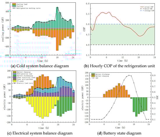
Figure 10.
Optimization results of Scenario 3.
Figure 10b shows the hourly COP of the cooling units under the typical daily operating mode for Scenario 3. From the figure, it can be seen that the cooling units operate only during the day, and their actual COP is mostly higher than the rated COP. The average COP reached 5.01, which validates the effectiveness of the cooling system’s design and operational optimization. Figure 10c presents the operational state of the park’s electrical system on a typical day. Observing the data above the y = 0 axis, after adding the cooling electrical load, the overall trend of the park’s electrical load is similar to the overall trend of other electrical loads excluding cooling, and its value is nearly twice that of the other electrical loads. In the absence of cold storage devices in the park system, a very high peak in the electrical load occurs between t = 18 and t = 20. The electrical load at the peak time is 2.08 times and 2.36 times that of the same time in Scenario 1 and Scenario 2, respectively. The comparison demonstrates that cold storage devices have a high energy scheduling capability. Additionally, due to the higher electrical load scheduling demand, the battery capacity in Scenario 3 is larger than that in Scenario 1. The battery stores a large amount of energy during the daytime when photovoltaic generation is abundant, in order to supply electricity during the evening when both the electricity demand and electricity price are at their peaks. Observing the data below the y = 0 axis, the photovoltaic modules start generating electricity at t = 5, reaching their peak generation at t = 12. The output then begins to decrease, and by t = 18, the photovoltaic modules no longer generate electricity. From this observation, it can be seen that the combination of the battery and photovoltaic system cannot fully meet the park’s electricity demand throughout the day. The system needs to purchase electricity from the grid during the periods from t = 0 to t = 5 and at t = 24. This is because the electricity price from the grid is at its lowest valley price during these times and is even slightly lower than the photovoltaic grid-connected price. To meet the park’s self-sufficiency during this period, a larger battery capacity and photovoltaic area would be required, resulting in negative economic benefits during this period. In simple terms, the grid can be viewed as a large battery: excess electricity during the day is sold to the grid, and electricity is purchased at the valley price during the night. The grid-connected price of 0.3598 CNY/kWh is higher than the valley price of 0.2996 CNY/kWh. Even ignoring the initial investment and maintenance costs of the battery, greater economic profit can be obtained compared to a plan with a higher battery capacity. Therefore, the optimized maximum battery capacity is 974 kWh.
The typical daily charge–discharge status and SOC of the battery are shown in Figure 10d. Throughout the entire cooling season, the battery operates in a charge–discharge cycle every 24 h, with the battery charging from t = 6 to t = 16 and discharging from t = 17 to t = 23. At the same time, the battery’s SOC remains within the range of 0.1 to 0.9 throughout the day, ensuring the health and stability of the battery. It also meets the maximum charge–discharge power of the battery, validating the rationality of the planning and operation of energy storage devices in the park system as proposed in this study. The total operating cost for the entire cooling season in this scenario is calculated to be CNY 83,740, with the total cost for the cooling season, including the initial purchase cost of the equipment, amounting to CNY 189,586. The operating cost on the typical day of July 10th is CNY 678, and the total daily cost, including the initial purchase cost, is CNY 1525. Under the operational mode of Scenario 3, the total carbon emission for the entire cooling season in the park is 7498 kgCO2e. The carbon emission on the typical day is 64 kgCO2e, and the overall photovoltaic consumption rate for the park reaches 95.77%, with a photovoltaic consumption rate of 100% on the typical day.
5.5. Scenario 4: PV Distributed System Without Energy Storage
Scenario 4 serves as a comparison scenario for the example, where a distributed photovoltaic energy storage system without energy storage is set up. The optimized configuration results for the system’s equipment capacity are shown in Table 5. From the table, it can be seen that the photovoltaic area is 894 m2, covering 39.38% of the park’s electricity demand. The cooling system selects a configuration of one 75 kW unit and three 140 kW units. Under this configuration, the cooling units can generally maintain high efficiency during operation. The typical daily operation status of the cooling system and the hourly COP of the cooling units in Scenario 4 are similar to those in Scenario 3. The operational status and COP of the cooling units can be referenced in Figure 10a,b. Figure 11 shows the operational status of the park’s electrical system on a typical day in Scenario 4. Observing the data above the y = 0 axis, since the cooling system is similar to Scenario 3, the electrical load in Scenario 4 exhibits the same characteristics as in Scenario 3, with a high peak load at the same time. However, due to the lack of energy storage devices, the excess photovoltaic generation in Scenario 4 can only be sold to the grid. Large-scale photovoltaic grid integration can destabilize the grid, and since the selling price is relatively low, expanding the photovoltaic area does not generate higher economic or environmental benefits. In other words, the park system without energy storage cannot achieve large-scale photovoltaic absorption. Observing the data below the y = 0 axis, it can be seen that the photovoltaic generation from t = 6 to t = 15 closely follows the curve of the park’s electrical load for this period, indicating that photovoltaic generation is efficiently utilized during this time. If the photovoltaic area is reduced, the photovoltaic generation will decrease, and the system will purchase more electricity from the grid, resulting in economic and environmental losses. On the other hand, expanding the photovoltaic area will cause a large amount of photovoltaic generation to be integrated into the grid, which could impact grid stability. Additionally, the revenue from selling electricity will not cover the investment and operational costs of expanding the area. Therefore, the optimized photovoltaic area in this scenario is 894 m2. The total operating cost for the entire cooling season in this scenario is calculated to be CNY 224,432, with the total cost for the cooling season, including the initial purchase cost of the equipment, amounting to CNY 260,265. The operating cost on the typical day of July 10th is CNY 1976, and the total daily cost, including the initial purchase cost, is CNY 2277. Under the operational mode of Scenario 4, the total carbon emission for the entire cooling season in the park is 66,796 kgCO2e. The carbon emission on the typical day is 606 kgCO2e, and the overall photovoltaic consumption rate for the park reaches 90.14%, with a photovoltaic consumption rate of 95.77% on the typical day.
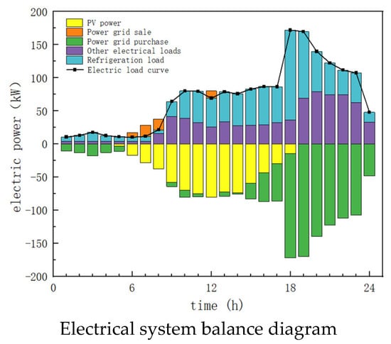
Figure 11.
Optimization results of Scenario 4.
5.6. Scenario 5: Distributed System for PV Energy Storage Without Bi-Level Optimization
Scenario 5 does not use the two-stage optimization model proposed in this paper. Instead, it adopts a planning and design phase followed by operational optimization based on the equipment configuration, meaning no iterative optimization between the planning design and scheduling operation phases. This scenario follows a traditional approach of determining the equipment configuration first and then performing optimization calculations based on that configuration. The optimized equipment capacity configuration results are shown in Table 5. The following provides the specific reasons for the selection of each equipment configuration.
Photovoltaic Area Setting: In order to meet the requirements for a zero-carbon park, where the photovoltaic generation needs to be greater than or equal to the total electrical load of the park, the park’s cooling load data are first divided by the COP to determine the approximate cooling electrical load. This paper uses a COP = 4 as the initial power for the cooling units. By adding this value to the other electrical loads in the park, the total electrical load of the park is obtained. The total electrical load is then filtered by day to identify the day with the highest load. The total photovoltaic generation for the entire day on the date with the highest load is calculated using a photovoltaic generation model. Based on the electrical load and the total daily generation per unit area, the required photovoltaic area is determined to be 2231 m2, which ensures that the photovoltaic generation is greater than or equal to the total electrical load of the park.
Refrigeration Unit Setting: The selection of the refrigeration units is based on the maximum cooling load in the park. Since, at certain times, both ice-making and cooling are required simultaneously, two refrigeration units are chosen to meet the respective cooling and ice-making needs. By analyzing the data, the date with the highest cooling load is identified as July 10th at 18:00, with a value of 493.64 kW. A 2% margin of error is added to the maximum cooling load, and two 250 kW refrigeration units, totaling 500 kW, are selected for this scenario.
Battery Setting: The battery capacity is determined based on the maximum electrical load during the park’s cooling season. From the data organized during the photovoltaic setting stage, the day with the highest electrical load is identified as August 2nd at 18:00, with a value of 189.36 kW. According to the electrical load data in this paper, the daily peak load generally occurs between t = 18 and t = 20. Therefore, the battery needs to fully meet the energy scheduling requirements for these 3 h. Additionally, to ensure the battery operates within a safe SOC range and can handle small-scale energy scheduling during other periods, the battery capacity is set to four times the maximum electrical load. The battery capacity is thus set to 757 kWh.
Ice Storage Tank Setting: The ice storage tank’s capacity is determined based on the maximum cooling load during the park’s cooling season. By analyzing the data, the date with the highest cooling load is identified as July 10th at 18:00, with a value of 493.64 kW. Following the principle used for the battery capacity setting, the capacity of the ice storage tank is set to four times the maximum cooling load. Therefore, the ice storage tank’s capacity is set to 1974 kWh.
The operational status of the cooling system under the optimal configuration is shown in Figure 12a. Compared with the cooling system balance diagram of Scenario 1, the main difference between the two scenarios is the operational mode at t = 3 and t = 4. Scenario 1 uses an ice storage tank cooling mode, while Scenario 5 uses a refrigeration unit cooling mode. This difference is due to the varying capacities of the ice storage tanks. By observing the COP curve of the cooling units in Figure 12b, it can be seen that the COP of the cooling units at t = 3 and t = 4 is very low, much lower than the rated COP. In Scenario 1, the ice storage tank cooling mode was adopted to avoid the increase in refrigeration electrical load when the cooling unit’s efficiency was very low. This indicates that Scenario 1 is superior to Scenario 5 in terms of ice storage tank capacity planning.
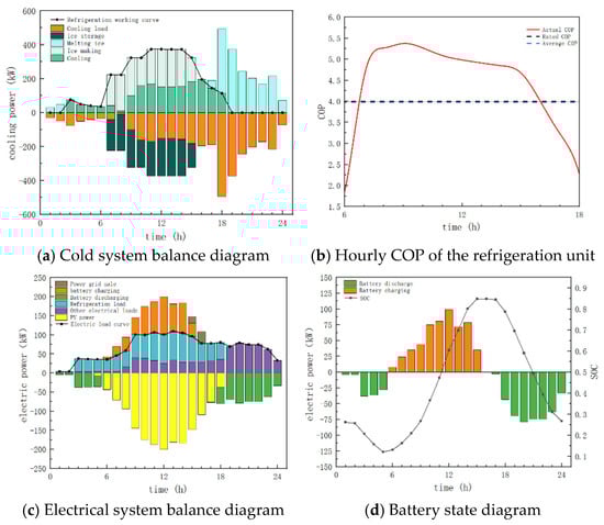
Figure 12.
Optimization results of Scenario 5.
Figure 12b shows the hourly COP of the cooling units under the typical daily operating mode. From the figure, it can be seen that the average actual COP of the cooling units is close to its rated COP, with a value of 3.97, which is 1.04 lower than that of Scenario 1 (5.01). This suggests that the cooling unit selection in Scenario 1 is superior to that in Scenario 5. Figure 12c shows the operational state of the park’s electrical system on a typical day in Scenario 5. By observing the data above the y = 0 axis and comparing them with the electrical system balance diagram of Scenario 1 in Figure 8a, two significant differences can be observed. The first difference is that the electrical load in Scenario 5 between t = 3 and t = 5 is much higher than in Scenario 1. This is due to the difference in cooling system operation modes mentioned earlier. During this period, a significantly higher electrical load is generated in Scenario 5 compared to Scenario 1, resulting in increased economic costs, scheduling pressure, and carbon emissions. The second difference occurs at t = 15 and t = 16, when the park system in Scenario 5 experiences electricity sales. This indicates that Scenario 1 has a better photovoltaic consumption rate than Scenario 5, thus proving that the photovoltaic area layout in Scenario 1 is superior to that in Scenario 5. By observing the data below the y = 0 axis, the main difference from Scenario 1 is also in the t = 3 to t = 5 period. During this time, the battery needs to discharge to meet the electricity demand, which increases the scheduling pressure on the battery. This indirectly validates that cold storage devices in the cooling system have a significant impact on the energy storage devices in the electrical system. The typical daily charge–discharge status and SOC of the battery are shown in Figure 12d. By observation, the main difference from Scenario 1 lies in the range of SOC values. In Scenario 1, the range is 0.102 to 0.898, while in Scenario 5, the range is 0.262 to 0.844. This indicates that the battery in Scenario 5 is not fully utilized compared to Scenario 1, meaning the battery capacity is set too large. Therefore, the battery capacity setting in Scenario 1 is superior to that in Scenario 5.
The total operating cost for the entire cooling season in this scenario is calculated to be CNY 91,976. The total cost for the cooling season, including the initial purchase cost of the equipment, is CNY 197,205. The operating cost on the typical day of July 10th is CNY 744, and the total daily cost, including the initial purchase cost, is CNY 1626. Under the operational mode of Scenario 5, the total carbon emissions for the entire cooling season in the park are zero. The overall photovoltaic consumption rate for the park reaches 95.92%, with a photovoltaic consumption rate of 97.07% on the typical day. The entire park achieves energy self-sufficiency.
5.7. Analysis of Economics and Carbon Emissions
5.7.1. Comparison of Environmental Benefits
Figure 13 illustrates the photovoltaic area layout for each scenario and their respective photovoltaic consumption rates on a typical day. From the figure, it can be seen that the photovoltaic consumption rate for each scenario is close to 100%, indicating that the equipment configuration in each scenario is reasonable, allowing for extensive use of the park’s photovoltaic generation without excessive energy waste. With a very high photovoltaic consumption rate, the photovoltaic area layout varies between scenarios, indicating that different equipment configurations influence the utilization of photovoltaic generation. A comparison between Scenario 4 and Scenarios 2 and 3 shows that both energy storage and cold storage modes can improve the park’s photovoltaic utilization capacity. Additionally, the energy storage mode has a greater advantage over the cold storage mode in enhancing photovoltaic utilization. A comparison between Scenario 1 and Scenarios 2 and 3 shows that the hybrid energy storage mode, combining both cold and energy storage, outperforms the single energy storage mode in enhancing photovoltaic utilization. The collaboration between cold and energy storage creates a positive impact, improving the park’s photovoltaic consumption capacity. A comparison between the results of Scenario 1 and Scenario 5 shows that the design and operation results obtained using the two-stage optimization method achieve a higher photovoltaic consumption rate compared to the traditional mode that does not involve iterations between the design and operation phases. This leads to a reduction in the photovoltaic area layout, thereby lowering initial investment and operational costs.
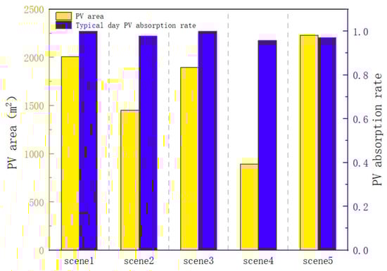
Figure 13.
Photovoltaic area and photovoltaic consumption rate in various scenarios.
Figure 14 shows the correlation between the park’s electricity consumption curve and the hourly photovoltaic generation curve for each scenario. In Scenario 1, through the synergy of cold storage and energy storage, the electricity consumption curve aligns very closely with the photovoltaic generation curve, with photovoltaic generation being fully utilized at all times. The consumption rate on a typical day reaches 100%. In Scenario 2, under the regulation of the cold storage mode, the electricity consumption curve fits closely with the photovoltaic generation curve from t = 0 to t = 18. However, due to limited scheduling capability, the two curves diverge significantly after t = 18, leading to a decrease in the photovoltaic area and consumption rate. The photovoltaic area is reduced by 27.76%, and the photovoltaic consumption rate decreases by 2.32%. In Scenario 3, the electricity consumption curve fits closely with the photovoltaic generation curve from t = 6 to t = 23, with a photovoltaic consumption rate of 100%. However, due to a high divergence during the nighttime period, the photovoltaic area is reduced by 5.62% compared to Scenario 1. In Scenario 4, the operation mode without energy storage results in the two curves fitting only during the midday period, with significant divergence at other times. As a result, the photovoltaic area and consumption rate drop significantly. In Scenario 5, the fit between the curves from t = 14 to t = 17 is lower than that in Scenario 1, demonstrating that the two-stage optimization method has a more significant advantage during the planning and design phase.
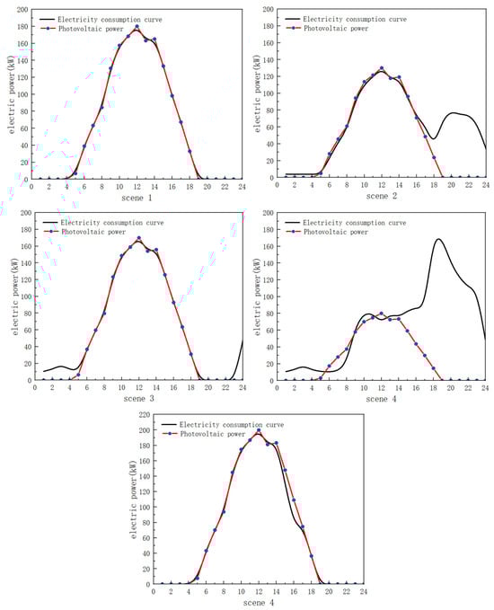
Figure 14.
Fitting of electricity consumption curves and PV curves in various scenarios.
The photovoltaic generation ratio refers to the proportion of total photovoltaic generation to the park’s total electrical load. It indicates the degree of clean energy supply in the park, which reflects the park’s zero-carbon level. Figure 15 shows the photovoltaic generation ratio and the total carbon emission for the cooling season in each scenario. It can be observed that the photovoltaic generation ratio is negatively correlated with carbon emissions. As the photovoltaic generation ratio increases, the park’s carbon emissions decrease. It can also be observed that the park with only an energy storage system has a higher photovoltaic generation ratio and lower carbon emissions compared to the park with only a cold storage system. The energy storage mode has a more efficient carbon reduction capability.
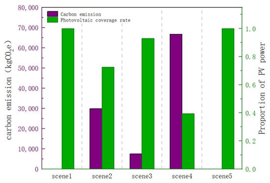
Figure 15.
Proportion of photovoltaic power generation and carbon emissions.
5.7.2. Comparison of Economic Benefits
First, a sensitivity analysis of electricity pricing strategies is conducted, as shown in Figure 16. For the first four scenarios using the bi-level optimization method, the park’s operating and investment costs are calculated with electricity prices increased or decreased by 20%, 40%, 60%, and 80%, and the comparison of total cost curves for each scenario is shown in Figure 17a. Scenarios 1 and 3 are less affected by price fluctuations because the two systems have stronger energy scheduling capabilities. As a result, even when electricity prices rise, the system can still maintain relatively low operating costs. On the other hand, in Scenario 2 and Scenario 4, due to the lack of energy storage devices, the energy scheduling capability is weaker, and overall operating costs increase almost linearly with the rise in electricity prices. Among these, Scenario 4, with no energy storage, has a steeper increase in operating costs, indicating that energy storage systems can effectively mitigate the impact of rising electricity prices on park expenses. Among these, the hybrid energy storage system, combining both energy and cold storage, has the most significant mitigating effect. The energy storage system is more effective than the cold storage system in alleviating the cost increases caused by higher electricity prices. From Figure 17a, it can be seen that when the electricity price exceeds 45.31% of the current price, the economic performance of the park system with energy storage is better than that of the system without energy storage. When the electricity price exceeds 74.29% of the current price, the economic performance of the energy storage park system is better than that of the cold storage park system. When the electricity price exceeds 54.78% of the current price, the economic performance of the hybrid energy storage and cold storage system is the best. As the electricity price increases, the economic differences between the four scenarios become more evident. The photovoltaic cost sensitivity analysis is shown in Figure 17b. By observing the slopes of the four curves, it is evident that scenarios with energy storage are more affected by changes in photovoltaic costs. Additionally, even with a 40% increase in photovoltaic costs, the energy storage scenarios maintain an economic advantage.
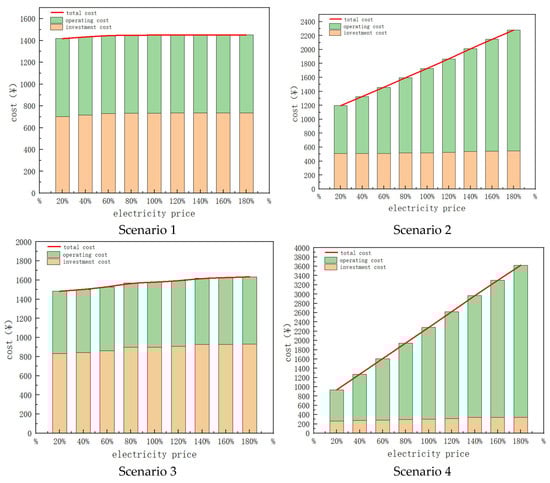
Figure 16.
Sensitivity analysis of electricity prices in various scenarios.
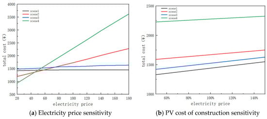
Figure 17.
Sensitivity analysis.
Figure 18 shows the operating costs for the cooling season and the total costs, including the initial investment, for each scenario. In Scenario 4, the park’s economic costs are the highest in the no-energy-storage mode. When cold storage devices are added, the operating costs and total costs decrease by 33.93% and 19.59%, respectively. When energy storage devices are added, the operating costs and total costs decrease by 62.69% and 27.16%, respectively. From an economic perspective, even considering the expensive initial investment costs, the economic performance of energy storage devices remains superior to that of cold storage devices. After the synergy between cold storage and energy storage, the operating costs and total costs decrease by 62.51% and 34.50%, respectively. Scenario 1 has 0.484% higher operating costs than Scenario 3, but its total costs are much lower than Scenario 3, reaching a reduction of 11.22%. This is because the initial investment cost of the battery is relatively high. The addition of the ice storage tank alleviates the energy scheduling pressure on the battery, reducing the design capacity of the battery. While slightly increasing operating costs, it significantly lowers the initial investment costs, maximizing the economic benefit. The synergy between cold storage and energy storage can have a positive economic impact. On one hand, the addition of the ice storage tank reduces the design capacity of the battery, mitigating the high investment costs of cold storage devices. On the other hand, the inclusion of the battery compensates for the insufficient regulation capability of the ice storage tank in the electrical system.
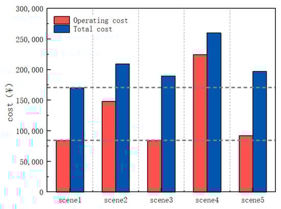
Figure 18.
Acting costs and total costs for each scenario.
Comparing the equipment configurations in Table 5, it can be seen that the total power of the cooling units in Scenario 1 is 390 kW, while in other scenarios, the cooling unit power ranges from 490 to 500 kW. The synergy between cold storage and energy storage can reduce the total power of the cooling units while maintaining their efficiency, resulting in lower system economic costs. Compared to Scenario 5, Scenario 1 has operating costs and total costs that are reduced by 8.51% and 13.56%, respectively. The two-stage optimization method also shows greater economic advantages compared to traditional planning methods.
6. Conclusions and Discussion
6.1. Conclusions Analysis
Through the comparative analysis of the above scenarios, the following conclusions can be drawn:
(1) The bi-level optimization model proposed in this paper efficiently utilizes green energy, fully tapping into the operational potential of the park’s equipment, achieving economic savings, environmental friendliness, and sustainable development. The coordinated scheduling of cold storage and energy storage in the park’s energy system improves system economics and reduces carbon emissions. The coordination of cold storage and energy storage also reduces the total power of the cooling units in the design phase, optimizes the operational state of the cooling units, and reduces the total electrical load and initial investment in the park. In comparison to the single energy storage mode, the energy storage mode outperforms the cold storage mode in both economic and environmental aspects, with operating costs and total costs decreasing by 43.53% and 9.41%, respectively. The significant reduction in operating costs is due to the energy storage system directly scheduling electricity, while the cold storage system indirectly influences the electrical cooling load through the impact on cooling energy, resulting in a relatively weaker scheduling capability and a noticeable difference in operating costs. The difference in total costs is relatively small because the energy storage system, compared to the cold storage system, has higher equipment investment costs.
(2) Compared to the traditional planning method, where the equipment configuration is first determined based on maximum load and then optimized for operation, the two-stage optimization planning method reduces operating costs and total costs by 8.51% and 13.56%, respectively. Despite a 9.91% reduction in the photovoltaic layout area, it still achieves the goal of zero carbon emissions. The overall photovoltaic consumption rate during the cooling season also increased by 2.45%, and the layout area of the photovoltaic system is more rational. Additionally, the total capacity of the cooling units has been reduced by 20.21%, while operational efficiency has improved by 26.07%. The selection and operation plan for the cooling units have been optimized for better efficiency. The design of the ice storage tanks and batteries also surpasses the traditional planning method, making the overall energy scheduling in the park more efficient and rational.
(3) The following suggestions are made regarding government policies: 1. From both an economic and environmental perspective, energy storage technologies should be vigorously developed, and parks should be encouraged to implement diversified and collaborative energy storage models. Special emphasis should be placed on developing energy storage technologies that offer stronger energy scheduling capabilities. 2. Fluctuations in electricity prices will affect the park’s system structure and economic costs. When electricity prices increase, it can promote the installation of renewable energy and the application of energy storage systems, thereby reducing carbon emissions in the park. Increasing the price differential in time-of-use pricing can have a similar effect. 3. Industrial upgrading should be carried out to reduce the purchase costs of renewable energy generation equipment and energy storage devices, thus promoting the park’s transition to a low-carbon model.
6.2. Discussion Analysis
This paper presents a preliminary study of the two-stage optimization method for park-level energy systems. However, there are some limitations with regard to certain aspects, and further research can be conducted in the following areas:
(1) In order to shorten the model calculation time, this study’s case study focuses only on the cooling season, which has the highest energy consumption in the park. Future work could extend the analysis to cover the entire year, dividing it into the cooling season, heating season, and transition seasons, and applying the two-stage optimization method to the whole year. This would provide a more comprehensive solution for the park’s energy system.
(2) The case study in this research is focused solely on the Beijing region of China. Due to limitations in resources, practical verification for other regions has not been conducted. Future plans include conducting comparative analysis under different climatic conditions to validate the model’s optimization effects in various regions.
(3) This study treats the park as a whole for the two-stage optimization analysis. Future research could focus on the thermal and electrical load characteristics of individual buildings within the park. By establishing scenarios that modify the load characteristics of each building, a comparative analysis can be conducted to study the impact of building load characteristics on the energy system design and operation of the park.
Author Contributions
Methodology, Y.G. (Yan Gao); Writing—original draft, Z.W. and Y.G. (Yaping Gao). All authors have read and agreed to the published version of the manuscript.
Funding
This research received no external funding.
Data Availability Statement
The original contributions presented in this study are included in the article. Further inquiries can be directed to the corresponding author.
Conflicts of Interest
The authors declare no conflicts of interest.
References
- Zhao, X.; Ma, X.; Chen, B.; Shang, Y.; Song, M. Challenges toward carbon neutrality in China: Strategies and countermeasures. Resour. Conserv. Recycl. 2022, 176, 105959. [Google Scholar] [CrossRef]
- Yu, Z.; Geng, Y.; Calzadilla, A.; Bleischwitz, R. China’s unconventional carbon emissions trading market: The impact of a rate-based cap in the power generation sector. Energy 2022, 255, 124581. [Google Scholar] [CrossRef]
- Cui, L.; Wang, J.; Chen, X.; Song, M. Regional policy options for carbon peaking in the Yangtze River Delta under uncertainty. J. Environ. Manag. 2024, 364, 121445. [Google Scholar] [CrossRef] [PubMed]
- Xia, W.; Apergis, N.; Bashir, M.F.; Ghosh, S.; Doan, B.; Shahzad, U. Investigating the role of globalization, and energy consumption for environmental externalities: Empirical evidence from developed and developing economies. Renew. Energy 2022, 183, 219–228. [Google Scholar] [CrossRef]
- Chen, Z.; Jiang, M.; Qi, L. Using existing infrastructures of high-speed railways for photovoltaic electricity generation. Resour. Conserv. Recycl. 2022, 178, 6091. [Google Scholar] [CrossRef]
- Wu, C.; Liu, P.; Cheng, Q.; Yang, Z.; Huang, K.; Liu, Z.; Zheng, Y.; Li, X. Analytical method for optimizing capacity expansion of existing hydropower plants in hydro-wind-photovoltaic hybrid system: A case study in the Yalong River basin. Appl. Energy 2025, 383, 125297. [Google Scholar] [CrossRef]
- Qiu, S.; Wu, X.; Lin, B.; Lin, P. Factors on regional installations of residential photovoltaics in China. Energy 2025, 316, 134524. [Google Scholar] [CrossRef]
- Wang, K.; Zhong, C.; Yu, R. The greenhouse gas reduction effect of critical peak pricing for industrial electricity: Evidence from 285 Chinese cities, 2003–2019. Energy Policy 2024, 190, 114–147. [Google Scholar] [CrossRef]
- Jordehi, A. Optimisation of demand response in electric power systems, a review. Renew. Sustain. Energy Rev. 2019, 103, 308–319. [Google Scholar] [CrossRef]
- Heylen, E.; Deconinck, G.; Hertem, D. Review and classification of reliability indicators for power systems with a high share of renewable energy sources. Renew. Sustain. Energy Rev. 2018, 97, 554–568. [Google Scholar] [CrossRef]
- Bahramara, S.; Parsa, M.; Moghaddam, M. Optimal planning of hybrid renewable energy systems using HOMER: A review. Renew. Sustain. Energy Rev. 2016, 62, 609–620. [Google Scholar] [CrossRef]
- Karunathilake, H.; Perera, P.; Ruparathna, R.; Hewage, K.; Sadiq, R. Renewable energy integration into community energy systems: A case study of new urban residential development. J. Clean. Prod. 2018, 173, 292–307. [Google Scholar] [CrossRef]
- Jung, J.; Villaran, M. Optimal planning and design of hybrid renewable energy systems for microgrids. Renew. Sustain. Energy Rev. 2017, 75, 180–191. [Google Scholar] [CrossRef]
- Fujisawa, K.; Fujisawa, Y.; Waki, H. Approaches to Optimal Design and Operation of Distributed Energy Systems. In Optimization in the Real World: Toward Solving Real-World Optimization Problems; Springer: Tokyo, Japan, 2016; pp. 157–176. [Google Scholar] [CrossRef]
- Quashie, M.; Marnay, C.; Bouffard, F.; Joós, G. Optimal planning of microgrid power and operating reserve capacity. Appl. Energy 2018, 210, 1229–1236. [Google Scholar] [CrossRef]
- Zhang, Y.; Campana, P.; Lundblad, A.; Zheng, W.; Yan, J. Planning and operation of an integrated energy system in a Swedish building. Energy Convers. Manag. 2019, 199, 111920. [Google Scholar] [CrossRef]
- Zhang, Y.; Xiao, S.; Han, Y. An MILP (mixed integer linear programming) model for optimal design of district-scale distributed energy resource systems. Energy 2015, 90, 1901–1915. [Google Scholar]
- Shen, H.; Zhang, H.; Xu, Y.; Chen, H.; Zhu, Y.; Zhang, Z.; Li, W. Multi-objective capacity configuration optimization of an integrated energy system considering economy and environment with harvest heat. Energy Convers. Manag. 2022, 269, 116116. [Google Scholar] [CrossRef]
- Zare, M.; Narimani, M.; Malekpour, M.; Terzija, V. Reserve constrained dynamic economic dispatch in multi-area power systems: An improved fireworks algorithm. Int. J. Electr. Power Energy Syst. 2021, 126, 106579. [Google Scholar] [CrossRef]
- Li, C.; Yang, Y.; Wang, Z.; Wang, N.; Wang, L.; Yang, Z. Energy hub-based optimal planning for integrated energy systems considering part-load characteristics and synergistic effect of equipment. Glob. Energy Interconnect. 2021, 4, 169–183. [Google Scholar] [CrossRef]
- Huang, W.; Zhang, N.; Wang, Y.; Capuder, T.; Kang, C. Matrix modelingof energy hub with variable energy efficiencies. Int. J. Electr. Power Energy Syst. 2019, 119, 105876. [Google Scholar] [CrossRef]
- Kong, X.; Gao, J.; Zhang, D.; Li, W.; Gao, X. Flexible and adjustable resource backup capacity planning method for port areas with a high percentage of new energy access. Electr. Power Syst. Res. 2025, 241, 111265. [Google Scholar] [CrossRef]
- Heidari, A. Stochastic effects of ice storage on improvement of an energy hub optimal operation including demand response and renewable energies. Appl. Energy 2020, 261, 114393. [Google Scholar] [CrossRef]
- Zhao, L.; He, D.; Zeng, X.; Wu, J. Distributed Photovoltaic Energy Storage Configuration Method for Distribution Network Considering Voltage Constraint. In Proceedings of the Big Data and Artificial Intelligence (ICIBA), Chongqing, China, 26–28 May 2023; pp. 485–489. [Google Scholar]
- Yu, H.; Yong, X. Double-layer planning configuration with distributed PV power and energy storage system. In Proceedings of the 2022 IEEE 5th International Conference on Automation, Electronics and Electrical Engineering (AUTEEE), Shenyang, China, 18–20 November 2022; pp. 37–41. [Google Scholar]
- Li, J.; Zhang, Y.; Chen, C.; Wang, X.; Shao, Y.; Zhu, X.; Li, C. Two-Stage Planning of Distributed Power Supply and Energy Storage Capacity Considering Hierarchical Partition Control of Distribution Network with Source-Load-Storage. Energy Eng. 2024, 121, 2389. [Google Scholar] [CrossRef]
- Ding, Y.; Wei, X. Bi-level optimization model for regional energy system planning under demand response scenarios. J. Clean. Prod. 2021, 323, 129009. [Google Scholar] [CrossRef]
- Liao, J.; Lin, J.; Wu, G. Two-layer optimization configuration method for distributed photovoltaic and energy storage systems based on IDEC-K clustering. Energy Rep. 2024, 11, 5172–5188. [Google Scholar] [CrossRef]
- GB/T 51350-2019; Technical Standard for Nearly Zero Energy Buildings. Ministry of Housing and Urban Rural Development of the People’s Republic of China: Beijing, China, 2019.
Disclaimer/Publisher’s Note: The statements, opinions and data contained in all publications are solely those of the individual author(s) and contributor(s) and not of MDPI and/or the editor(s). MDPI and/or the editor(s) disclaim responsibility for any injury to people or property resulting from any ideas, methods, instructions or products referred to in the content. |
© 2025 by the authors. Licensee MDPI, Basel, Switzerland. This article is an open access article distributed under the terms and conditions of the Creative Commons Attribution (CC BY) license (https://creativecommons.org/licenses/by/4.0/).