A Model Predictive Control to Improve Grid Resilience

Abstract

The following article details a model predictive control (MPC) to improve grid resilience when faced with variable generation resources. This topic is of significant interest to utility power systems where distributed intermittent energy sources will increase significantly and be relied on for electric grid ancillary services. Previous work on MPCs has focused on narrowly targeted control applications such as improving electric vehicle (EV) charging infrastructure or reducing the cost of integrating Energy Storage Systems (ESSs) into the grid. In contrast, this article develops a comprehensive treatment of the construction of an MPC tailored to electric grids and then applies it integration of intermittent energy resources. To accomplish this, the following article includes a description of a reduced order model (ROM) of an electric power grid based on a circuit model, an optimization formulation that describes the MPC, a collocation method for solving linear time-dependent differential algebraic equations (DAEs) that result from the ROM, and an overall strategy for iteratively refining the behavior of the MPC. Next, the algorithm is validated using two separate numerical experiments. First, the algorithm is compared to an existing MPC code and the results are verified by a numerically precise simulation. It is shown that this algorithm produces a control comparable to existing algorithms and the behavior of the control carefully respects the bounds specified. Second, the MPC is applied to a small nine bus system that contains a mix of turbine-spinning-machine-based and intermittent generation in order to demonstrate the algorithm’s utility for resource planning and control of intermittent resources. This study demonstrates how the MPC can be tuned to change the behavior of the control, which can then assist with the integration of intermittent resources into the grid. The emphasis throughout the paper is to provide systematic treatment of the topic and produce a novel nonlinear control compatible design framework applicable to electric grids and the control of variable resources. This differs from the more targeted application-based focus in most presentations.

1. Introduction

This paper presents a MPC to assist in the robust, adaptive, and resilient control of the electric power grid (EPG). Given the increasing number of distributed intermittent sources, the control and stability of the EPG is of significant interest to utility power systems. Currently, the EPG maximizes the spinning inertia of fossil fuel generators in order to provide the energy storage necessary to meet stability and performance requirements [1]. This paper formulates an MPC to control grid, which has replaced a large amount of the spinning inertia from fossil fuel generators with intermittent energy resources.

In order to efficiently control the grid’s inertia, the grid requires multiple types of controls. For rapidly changing behavior, the grid requires real-time feedback controls that range from simple droop controls to more sophisticated Hamiltonian Surface Shaping and Power Flow Controls (HSSPFC) [2]. Although these types of controls can be used to transition the grid from one operating state to another through the use of gain scheduling, they are typically best suited for maintaining a given operating condition and stability. To transition the grid from one state to another, such as during an outage or cold start, an MPC is better suited. An MPC is a type of optimal feedforward control that generates a trajectory that guides the system from one operating condition to another. It does so by solving an optimization formulation based on a mathematical model of the system. This allows a performance metric, such as use of energy storage, to be minimized while satisfying the dynamics as well as any initial and terminal conditions. Note, this kind of control can also be combined with a feedback control to help track the computed trajectory. This can be accomplished by backsubstituting the MPC into the dynamics used when generating the feedback controller or when computing the stability analysis. That said, since this introduces a time-dependent quantity into the dynamics, such stability analysis is significantly more complicated than it would be for a time-independent system.

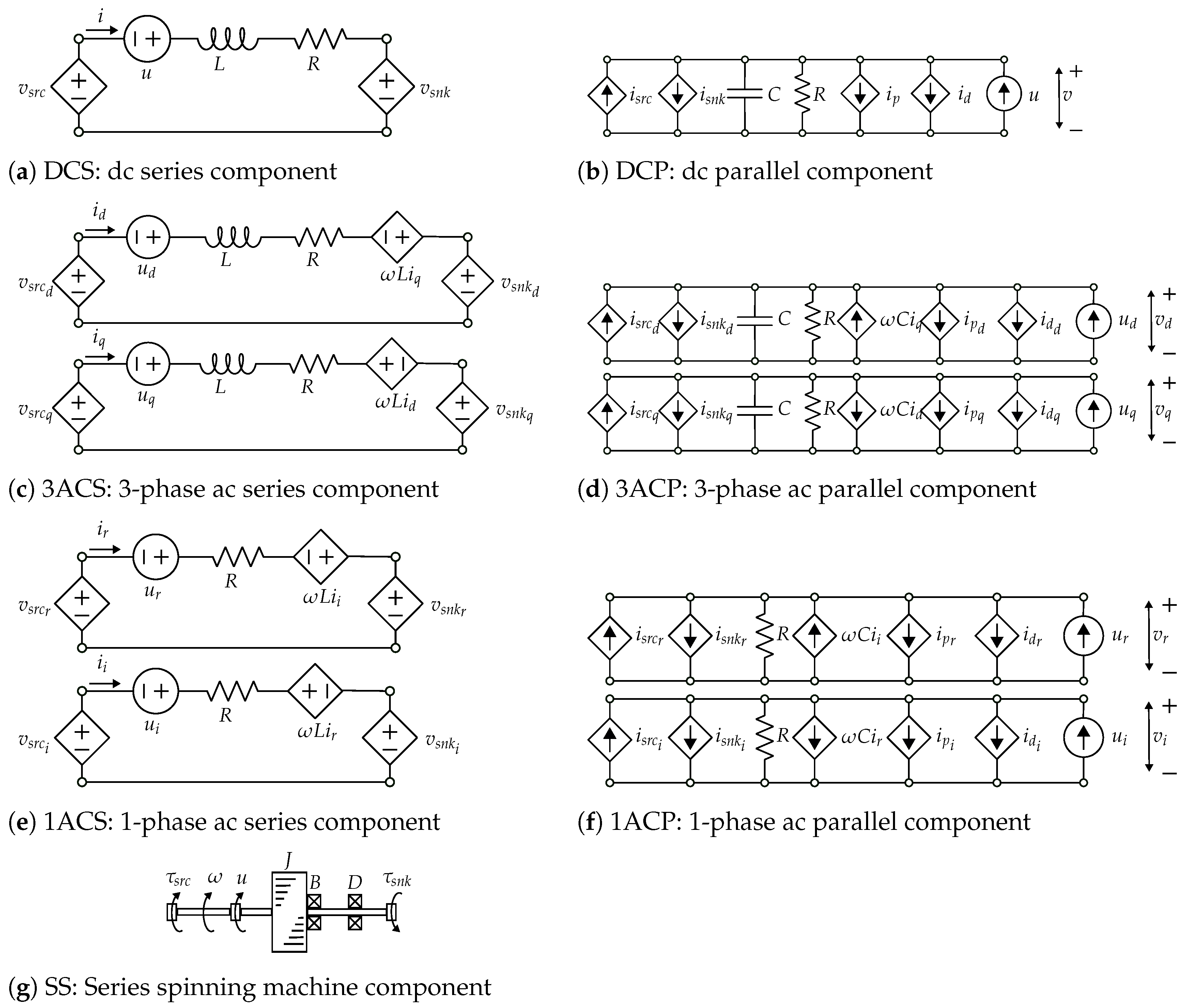
To build an MPC, the formulation requires both a ROM as well as an optimization formulation built on this model. Further, since a study of how to supplement the inertia from fossil fuel generators necessarily requires multiple grid configurations, the ROM necessarily needs to be built from a set of flexible components that can not only integrate well into an optimization formulation, but can quickly represent a new grid. To this end, there are three different modeling techniques broadly applicable to the analysis, planning, and operation of an electric grid: Ybus complex algebraic models, full time-domain three-phase circuit models, and d-q domain circuits.

In the Ybus complex algebraic model, a network’s self- and mutual-admittance at each node is represented in a bus admittance matrix [3,4]. Then, these admittances are used to solve the power flow equations, which relate bus voltages and power injections. This approach has applications in the planning and operation of power systems, voltage regulation studies, contingency analysis, and economic dispatch. However, it also assumes balanced three-phase systems, neglects dynamic phenomena like transients and harmonics, and does not accurately model nonlinear loads or devices. Software that uses this approach includes PowerWorld Simulator V24 [5], PSS/E 35.4 [6], and ETAP 2024 [7].

In the full time-domain three-phase circuit models, also known as Electro-Magnetic Transient (EMT) models, all power system components are represented using detailed circuit models [4,8]. This includes transmission lines (distributed parameter models), transformers (detailed equivalent circuits), generators, loads, and power electronic devices (switching functions and nonlinear characteristics). This approach has applications in transient stability analysis, harmonic analysis, insulation coordination studies, protection system design, and the analysis of fast switching events. However, these models also have a high computational burden, especially for large power systems, require accurate and detailed models of all system components, and the simulation times can be long, especially for complex systems. Software that uses this approach includes PSCAD V5 [9], ATP 2024 [10], and RTDS [11].

In the d-q domain circuits, the Park transform is used to transform three-phase ac quantities such as voltages and currents into dc quantities in a rotating reference frame [4,12]. This helps to simplify the analysis of synchronous and induction machines by eliminating the time-varying inductances, which allows for simpler and more efficient control algorithms. It also facilitates the control of power electronic converters by transforming ac quantities into dc quantities, enabling the use of simpler control strategies, such as PI controllers. This approach has applications in the control of synchronous generators and induction motors, the control of voltage source converters (VSCs) and other power electronic devices, and the analysis of power system stability. However, these models also require a thorough understanding of the Park transformation and its implications, can be complex to apply to systems with multiple rotating reference frames, and add a layer of complexity to the overall system view. Software that uses this approach includes MATLAB/Simulink R2024B [13], PSCAD V5 [9], and PowerFactory 2025 [14].

Modern power system analysis often involves a combination of these modeling techniques. Load flow analysis (Ybus) is used for initial planning and steady-state studies; EMT simulations are used for detailed transient analysis and protection system design; and, d-q domain models are used for the control and analysis of rotating machines and power electronic converters. With the rise of intermittent energy sources and smart grids, the importance of dynamic modeling and control is increasing, making EMT and d-q domain models increasingly essential. Hybrid simulations combining different model types are also becoming more common.

The emphasis in this paper is on the development of a flexible framework to quickly represent a combination of dc, 3-phase ac, and steady state 1-phase ac grids interconnected to multiple spinning machines. As a result, this paper uses and presents d-q domain circuits and related models for its ROM. This framework also requires a variety of additional modeling capabilities such as high-order bounds to constrain the ROMs behavior and flexible objective functions to shape the control.

In order to satisfy these goals, this article presents a continuous time, nonlinear MPC based on a full-space optimization formulation that has been discretized using an orthogonal spline collocation (OSC) method based on a discretize-then-optimize approach. Since bounding the behavior of the system is critical to its safety and performance, the MPC enables a combination of both nonlinear and constant bounds. Further, these bounds may be applied to either the state or control variables, bound the variable itself or its high-order derivatives, and are satisfied over the entire time horizon and not just at a discrete set of points. This allows properties such as the ramp rate to be bounded and ensures a bound is obeyed between the controller’s sample time. Finally, the algorithm enables multiple model fidelities between the variables, which allows independent refinement between the state and control variables. This makes it possible to accurately solve for the state of the system when there is a rapidly varying control.

Due to their success, many other MPC packages exist. For instance, GPOPS-II [15] provides a continuous time MPC discretized using a collocation method. Their approach and this paper both use a collocation method, implement a continuous time control, and enable adaptive mesh refinement. The algorithms differ in the type of polynomials used in the discretization, which also impacts the location of the collocation points. Further, GPOPS-II only enforces the bounds at the collocation points and not over the entire domain. Alternatively, pyomo.DAE [16] provides a discrete time MPC based on either a collocation method or finite differences. Their approach and this paper both implement a collocation method and enable adaptive mesh refinement. However, similar to GPOPS-II, the algorithms differ in the type of polynomials used in the discretization, which impacts the location of the collocation points. It also only enforces the bounds at the collocation points and not over the entire domain. Further, it produces a discrete, not continuous time control. Finally, MathWorks provides the Model Predictive Control Toolbox [17]. This algorithm and the toolbox differ in the type of discretization used. The MPC Toolbox implements Tustin’s method, a type of implicit trapezoidal rule, which generates a discrete time control. This also requires the control and state variables to be solved on the same time fidelity and only allows for bounds to be enforced at a discrete set of points.

For an overall survey of the use of MPCs with microgrids, Villalón et al. [18] and Tumeran et al. [19] provide a good summary. Of note, Ryu et al. developed an MPC for improving the hosting capacity of photovoltaics (PVs) and EVs in a stand-alone microgrid. They used a discrete time circuit-based model that determined the optimal usage of the ESS. Although both this paper and their research use a circuit-based ROM, the actual model used differs. In addition, this paper presents a more general framework for an MPC tailored to an electric grid, which includes additional details on how the MPC is discretized and constructed. In [20], Kong, Liu, Ma, and Lee presented a hierarchical model predictive control to reduce the cost of integrating wind, solar, and battery power into the grid. Similar to this paper, they use a d-q electrical model combined with a mechanical model for their ROM. This papers differs from theirs in its aim and scope. The focus here is to develop an MPC tailored to an general electric grid, which includes additional details on how the MPC is constructed and solved. Finally, Legry et al. present an MPC for controlling the state of charge of an ESS on an islanded microgrid [21]. As with this paper, the control and use of an ESS is modeled and controlled. However, their work differs from this paper in that they use a Ybus algebraic model rather than a d-q circuit-based model. Broadly, what distinguishes this paper from the others is in the detail provided in how to construct an MPC targeted toward electrical microgrids.

The paper is outlined as follows. First, the article describes a reduced order model (ROM) of an electric power grid based on a circuit model. The goal of this section is to provide a mathematical framework for modeling the grid and to develop a set of abstractions that integrate well into an MPC. Second, the article details an optimization formulation that describes the MPC. This formulation is built on the aforementioned ROM and introduces various objectives to control the behavior of the MPC. Third, the article describes a collocation method for solving linear time-dependent differential algebraic equations (DAEs). This algorithm is required for solving the stiff differential equations that result from the ROM and is designed to integrate efficiently into an MPC. Next, a set of strategies are presented for refining the behavior the MPC. Since each solution to the MPC formulation can be considered optimal, it is important to understand how to alter the behavior of the MPC to achieve the desired result. Finally, the article demonstrates the efficacy of the approach with two different numerical experiments. In the first, the approach is validated against another MPC code for a small electrical microgrid. Then, the result from both codes is used in a high-precision numerical simulation to validate their performance. In the second, the MPC is applied to a small nine bus system that contains a mix of turbine-based and intermittent generation. The purpose here is to demonstrate that the framework developed within this paper can assist in the control and design of intermittent resources.

2. Model

2.1. Background

This paper models an electric grid using a ROM based on circuit components using an averaged-switch model. The purpose here is to choose a ROM with higher fidelity than a power flow model, but without the discontinuities inherent to switching models. Although this formulation can be used independently of an MPC, care has been taken to construct a model that integrates easily into an optimization solver.

These models extend and expand the models described by Young, Wilson, Cook, Weaver, and Glover in [22] and Young, Wilson, Weaver, and Robinett in [23] by adding steady state 1-phase ac components. In addition, this paper uses a more general form of the model that better integrates with other power system components and abstractions, which allows for a more unified framework. In addition, this article uses a modified per-unit modeling scheme compatible with the ROM. This is necessary since the ROM used here differs from a more traditional power flow model and the scaling for the scenarios solved in this paper requires it. Namely, this ROM also tracks the amount of energy in an energy storage device, which requires a minor variation to transform into a per-unit form consistent with power.

2.2. Components vs. Connections

Overall, the ROM divides the circuit into two kinds of elements: components and connections. The power system components can be found in Figure 1 and the state equations for these components can be seen in

Table 1. State equations for the grid components in Figure 1.

Dc Components
Series bus (DCS)	$L{i}^{\prime }+Ri+v_{\mathit{snk}}=v_{\mathit{src}}+u$
Series energy storage	$w^{\prime }=-ui$
Parallel bus (DCP)	$C{v}^{\prime }+v/R+\sum i_p+\sum i_d+\sum i_{\mathit{snk}}=\sum i_{\mathit{src}}+u$
Parallel non-dispatchable load *	$i_p=P/v$
Parallel dispatchable load *	$i_d=d/v$
Parallel energy storage	$w^{\prime }=-vu$
3-phase ac components
Series bus (3ACS)	$L{i}_d^{\prime }+R{i}_d-\omega L{i}_q+v_{{\mathit{snk}}_d}=v_{{\mathit{src}}_d}+u_d$
	$L{i}_q^{\prime }+R{i}_q+\omega L{i}_d+v_{{\mathit{snk}}_q}=v_{{\mathit{src}}_q}+u_q$
Series energy storage	$w^{\prime }=-u_d{i}_d-u_q{i}_q$
Series storage reactive power	$q=u_d{i}_q-u_q{i}_d$
Parallel bus (3ACP)	$C{v}_d^{\prime }+v_d/R-\omega C{v}_q+\sum i_{p_d}+\sum i_{d_d}+\sum i_{{\mathit{snk}}_d}=\sum i_{{\mathit{src}}_d}+u_d$
	$C{v}_q^{\prime }+v_q/R+\omega C{v}_d+\sum i_{p_q}+\sum i_{d_q}+\sum i_{{\mathit{snk}}_q}=\sum i_{{\mathit{src}}_q}+u_q$
Parallel non-dispatchable load *	$i_{p_d}=P{v}_d/(v_d^2+v_q^2)$
	$i_{p_q}=P{v}_q/(v_d^2+v_q^2)$
Parallel dispatchable load *	$i_{d_d}=d{v}_d/(v_d^2+v_q^2)$
	$i_{d_q}=d{v}_q/(v_d^2+v_q^2)$
Parallel energy storage	$w^{\prime }=-v_d{u}_d-v_q{u}_q$
Parallel storage reactive power	$q=v_d{u}_q-v_q{u}_d$
Steady state 1-phase ac components
Series bus (1ACS)	$R{i}_r-\omega L{i}_i+v_{{\mathit{snk}}_r}=v_{{\mathit{src}}_r}+u_r$
	$R{i}_i+\omega L{i}_r+v_{{\mathit{snk}}_i}=v_{{\mathit{src}}_i}+u_i$
Series energy storage	$w^{\prime }=-u_r{i}_r-u_i{i}_i$
Series storage reactive power	$q=u_r{i}_i-u_i{i}_r$
Parallel bus (1ACP)	$v_r/R-\omega C{v}_i+\sum i_{p_r}+\sum i_{d_r}+\sum i_{{\mathit{snk}}_r}=\sum i_{{\mathit{src}}_r}+u_r$
	$v_i/R+\omega C{v}_r+\sum i_{p_i}+\sum i_{d_i}+\sum i_{{\mathit{snk}}_i}=\sum i_{{\mathit{src}}_i}+u_i$
Parallel non-dispatchable load *	$i_{p_r}=P{v}_r/(v_r^2+v_i^2)$
	$i_{p_i}=P{v}_i/(v_r^2+v_i^2)$
Parallel dispatchable load *	$i_{d_r}=d{v}_r/(v_r^2+v_i^2)$
	$i_{d_i}=d{v}_i/(v_r^2+v_i^2)$
Parallel energy storage	$w^{\prime }=-v_r{u}_r-v_i{u}_i$
Parallel storage reactive power	$q=-v_r{u}_i+v_i{u}_r$
Spinning machine components
Series (SS)	$J{\omega }^{\prime }+B\omega +D(\omega -\overline{\omega })+{\tau }_{\mathit{snk}}={\tau }_{\mathit{src}}$
Series converter phase match	${\theta }^{\prime }=\omega -\overline{\omega }$
Series energy storage	$w^{\prime }=-u\omega$

Note, equations labeled with * are purely notational and do not introduce additional state variables. These variables can be simply substituted into the other equations.

. The state equations for the connections are in

Table 2. State equations for the grid connections that interconnect the components in Figure 1.

Source/Sink
Connection *	$v_{\mathit{src}/\mathit{snk}}=v_{\mathit{state}}$
Constant *	$v_{\mathit{src}/\mathit{snk}}=c$
Variable *	$v_{\mathit{src}/\mathit{snk}}=v_{\mathit{var}}$
Power *	$v_{\mathit{src}/\mathit{snk}}=P/v_{\mathit{state}}$
Transformers
Transformer (TR) *	$v_{\mathit{src}}=K\lambda v_{\mathit{snk}}$
	$i_{\mathit{snk}}=K\lambda i_{\mathit{src}}$
	$\lambda \ge 0$
Gyrator (GY) *	$v_{\mathit{src}}=K\lambda i_{\mathit{snk}}$
	$v_{\mathit{snk}}=K\lambda i_{\mathit{src}}$
	${\sum }_{k=1}^m{\lambda }_k=1$
	${\lambda }_k\ge 0$
Selector (SE) *	$v_{\mathit{src}}=K{\sum }_{k=1}^m{\lambda }_k{v}_{{\mathit{snk}}_k}$
	$i_{{\mathit{snk}}_k}=K{\lambda }_k{i}_{\mathit{src}}$
	${\lambda }_k\ge 0$
Power Converters
3-phase ac to dc converter (3AC/DC) *	$v_{{\mathit{src}}_d}=\sqrt{3/2}\cos \left(\theta \right)v_{\mathit{snk}}$
	$v_{{\mathit{src}}_q}=\sqrt{3/2}\sin \left(\theta \right)v_{\mathit{snk}}$
	$i_{\mathit{snk}}=\sqrt{3/2}(\cos \left(\theta \right)i_{{\mathit{src}}_d}+\sin \left(\theta \right)i_{{\mathit{src}}_q})$
Dc to 3-phase ac converter (DC/3AC) *	$v_{\mathit{src}}=\sqrt{3/2}(\cos \left(\theta \right)v_{{\mathit{snk}}_d}+\sin \left(\theta \right)v_{{\mathit{snk}}_q})$
	$i_{{\mathit{src}}_d}=\sqrt{3/2}\cos \left(\theta \right)i_{\mathit{src}}$
	$i_{{\mathit{src}}_q}=\sqrt{3/2}\sin \left(\theta \right)i_{\mathit{src}}$
Steady state 1-phase ac to dc converter (1AC/DC) *	$v_{{\mathit{src}}_r}=\cos \left(\theta \right)v_{\mathit{snk}}$
	$v_{{\mathit{src}}_i}=\sin \left(\theta \right)v_{\mathit{snk}}$
	$i_{\mathit{snk}}=\cos \left(\theta \right)i_{{\mathit{src}}_r}+\sin \left(\theta \right)i_{{\mathit{src}}_i}$
Dc to steady state 1-phase ac converter (DC/1AC) *	$v_{\mathit{src}}=\cos \left(\theta \right)v_{{\mathit{snk}}_r}+\sin \left(\theta \right)v_{{\mathit{snk}}_i}$
	$i_{{\mathit{src}}_r}=\cos \left(\theta \right)i_{\mathit{src}}$
	$i_{{\mathit{src}}_i}=\sin \left(\theta \right)i_{\mathit{src}}$
Active Power in Connection
3-phase ac to 3-phase ac	$p=(v_d{i}_d+v_q{i}_q)\lambda$
3-phase ac to dc	$p=3/2(v_d\cos \left(\theta \right)+v_q\sin \left(\theta \right))i\lambda$
Steady state 1-phase ac to 1-phase ac	$p=(v_d{i}_d+v_q{i}_q)\lambda$
Steady state 1-phase ac to dc	$p=(v_d\cos \left(\theta \right)+v_q\sin \left(\theta \right))i\lambda$
Reactive Power in Connection
3-phase ac to 3-phase ac	$q=(v_d{i}_q-v_q{i}_d)\lambda$
3-phase ac to dc	$q=3/2(v_d\sin \left(\theta \right)-v_q\cos \left(\theta \right))i\lambda$
Steady state 1-phase ac to 1-phase ac	$q=(v_d{i}_q-v_q{i}_d)\lambda$
Steady state 1-phase ac to dc	$q=(v_d\sin \left(\theta \right)-v_q\cos \left(\theta \right))i\lambda$

Note, equations labeled with * are purely notational and do not introduce additional state variables. These variables can be simply substituted into the other equations.

. Here, the division is chosen to allow for a general, flexible framework for constructing a grid. Note, equations labeled with * are purely notational and do not introduce additional state variables. These variables can be simply substituted into the other equations.

2.3. Series/Parallel Electrical Components

The power system components in Table 1 are themselves divided into series and parallel varieties and support dc, 3-phase ac, and steady state 1-phase ac grids. Each of these components can be used in multiple ways depending on kind of model required. For example, a simple model for solar generation can use a dc series component where the source voltage is set to a controlled voltage source, $v_{\mathit{src}}=P/i$. Then, P can be set to a prediction of the amount of power the solar array generates throughout the day. The voltage produced by the array can also be bounded to an expected, nominal level. Alternatively, the series components can be used to model a short line model of a transmission line, which neglects the line capacitance. As far as the parallel components, they naturally interconnect multiple transmission lines and provide a convenient location to model loads. Here, the non-dispatchable loads remove a specified amount of active power from the system whereas the dispatchable loads introduce a control variable, d, that allows for power shedding.

2.4. Spinning Machines

In addition to the purely electric components, the ROM in Table 1 includes a component for a spinning machine. This component largely uses the same formulation as the series dc component, which allows most of the implementation code to be reused. However, it contains an additional, optional damping term, $D(\omega -\overline{\omega })$, which helps synchronize the frequency of a spinning machines to a reference machine. In this context, $\overline{\omega }={\omega }_{\mathit{ref}}$. Alternatively, $\overline{\omega }$ can be set to a constant value. On the reference machine, this can help synchronize the frequency to a value such as 60 $\mathrm{Hz}$.

2.5. Ac Electrical Components

The 3-phase ac components in Table 1 fix the angular frequency, $\omega$, whereas the steady state 1-phase ac components allow it to vary as a state variable. Commonly, the angular frequency in the steady state 1-phase ac components is set to the angular frequency of a reference spinning machine connected to the grid. The 3-phase ac components are specified in a dq0 reference frame, which simplifies the modeling. Conversely, the steady state 1-phase ac components use a real embedding of the complex current and voltage written in Cartesian coordinates. In other words, a complex voltage is written as $v=v_r+i{v}_i$ and any complex state equations are divided into real and imaginary parts and solved separately. This is equivalent to using phasors, but produces a set of equations similar to those that result from a dq0 transform, albeit steady state. Practically, this means a carefully written piece of code can model dc, 3-phase ac, steady state 1-phase ac, and spinning machines using the same constructs.

2.6. Energy Storage

Each component in Table 1 can add an optional amount of energy storage through the controlled source, u. Then, the amount of energy stored is integrated from the active power into the state variable, w. The sign convention uses positive power to represent power delivered to the grid whereas negative power is power stored in the energy storage device. In the ac components, reactive power is optionally calculated as a separate algebraic variable. This allows the amount of reactive power to be bounded or penalized and helps to prevent instances of circulating reactive power.

2.7. Connections

Grid components may be connected directly or through the use of the transformers in Table 2. Here, the transformer acts like an ideal transformer where the control $\lambda$ represents the voltage ratio. This can also be seen as a boost or buck converter. The gyrator acts like the transformer, but allows a parallel component to be connected to a parallel component. Similarly, it allows a series component to be connected to a series. Here, the constant K can be used to convert to the appropriate units. For example, when a series spinning machine is connected to a series dc component, then K represents the machine torque constant, $K:$$\mathrm{N}\mathrm{m}{\mathrm{A}}^{-1}$. Next, the selector divides either current or voltage between different components. This allows, for example, 60% of the current to be sent to one component and 40% to another. As a final note, none of these connections generate additional state equations. Rather, they are embedded into the components above.

When components that use different kinds of power are connected to each other, such as dc to 3-phase ac, the power converters in Table 2 must be used. Similar to the transformers, these expressions are used directly within the components above. The converters are designed to preserve active power across the connection and can be combined with the transformers.

2.8. Active/Reactive Power

In addition to power conversion, the amount of active power moving through the connection and the amount of reactive power at the connection can be introduced to the formulation using the algebraic equations in Table 2. By bounding or penalizing each quantity, the power factor can be indirectly controlled. This tends to work more effectively than bounding the power factor directly. The problem with directly controlling the power factor is that when the amount of apparent power is near zero, the control may need to work very rapidly to maintain a certain power factor when it does not matter practically. Limiting the amount of reactive power tends to be more effective.

2.9. Utility Equations/Bounds

Finally,

Table 3. Additional utility equations for the grid components in Figure 1.

Initial condition	$v^{\left(k\right)}\left(0\right)=v_{k_0}$
General bound	$v_{k_{\min }}\le v^{\left(k\right)}\le v_{k_{\max }}$
Multiplicative linkage	$v=(v_1^{\left(k\right)}-c_1)(v_2^{\left(k\right)}-c_2)$
3-phase magnitude	$v_m=\sqrt{2/3}\sqrt{v_d^2+v_q^2}$
Steady state 1-phase magnitude	$v_m=\sqrt{v_r^2+v_i^2}$
3-phase magnitude and phase	$v_d=\sqrt{3/2}{v}_m\cos \left(\theta \right)$
	$v_q=\sqrt{3/2}{v}_m\sin \left(\theta \right)$
Steady state 1-phase magnitude and phase	$v_r=v_m\cos \left(\theta \right)$
	$v_i=v_m\sin \left(\theta \right)$

gives a variety of other utilitarian equations that can be introduced into any state or control variable in the formulation. Note, some of equations, such as initial conditions on the state, are required for a problem to be well-posed. Here, the notation $v^{\left(k\right)}$ denotes a higher order derivative where $v^{\left(0\right)}=v$. Next, the multiplicative linkage equation allows multiple variables to be coordinated. For example, if $v=u_1{u}_2$ where u denotes a controlled current source associated with energy storage, then a bound of $v\ge 0$ forces two different energy storage device to charge or discharge simultaneously. This prevents one energy storage device from charging another. Additionally, even though the ROM models ac quantities in either the dq0 reference frame or in Cartesian coordinates, if the magnitude and/or the phase are desired, they can be introduced through additional algebraic equations. This allows quantities such as voltage on an ac bus to be bounded between two values. Finally, the ROM allows arbitrary bounds to be placed on both state and control variables. In this simple case, this allows quantities such as the bus voltage to be bounded. Bounding higher-order derivatives allows quantities such as the rate of charge and discharge of an energy storage device to be bounded.

2.10. Example

As an example, consider a simple model where a solar array is modeled as a series dc component and connected to a steady state 1-phase ac bus that contains a single load. In addition, let there be a single energy storage device on the ac bus. Using the components above, the model can be represented using Figure 2 and the dynamics for this model can be found in

Table 4. Dynamics for the grid described by Figure 2.

Solar array	$L{i}^{\prime }+Ri+\lambda (v_r\cos \left(\theta \right)+v_i\sin \left(\theta \right))=P_{\mathrm{src}}/i$
	$i\left(0\right)=i_0$
Ac bus	$v_r/R_B-\omega C{v}_i+P_{\mathit{load}}{v}_r/(v_r^2+v_i^2)=\lambda i\cos \left(\theta \right)+u_r$
	$v_r\left(0\right)=v_{r_0}$
	$v_i/R+\omega C{v}_r+P_{\mathit{load}}{v}_i/(v_r^2+v_i^2)=\lambda i\sin \left(\theta \right)+u_i$
	$v_i\left(0\right)=v_{i_0}$
Voltage magnitude bound	$v_m=\sqrt{v_r^2+v_i^2}$
	$v_{\mathit{min}}\le v_m\le v_{\mathit{max}}$
Energy storage	$w^{\prime }=-v_r{u}_r-v_i{u}_i$
	$w\left(0\right)=w_0$
	$w\ge 0$
Energy storage charge/discharge bound	$-p_{\mathit{max}}\le w^{\prime }\le p_{\mathit{max}}$

.

2.11. Per-Unit Modeling

In order to improve scaling during solves, the above ROM is also compatible with per-unit parameterizations with some minor changes to the typical transformation procedure. Recall, per-unit modeling transforms the parameters within a model, so that most have a near unit size. It accomplishes this by defining base values for apparent power, $S_{\mathit{base}}$, voltage, $V_{\mathit{base}}$, current, $I_{\mathit{base}}$, and impedance, $Z_{\mathit{base}}$, so that $S_{\mathit{base}}=V_{\mathit{base}}{I}_{\mathit{base}}$ and $V_{\mathit{base}}=I_{\mathit{base}}{Z}_{\mathit{base}}$. Then, the grid is divided and transformed by regions where the regions are defined by the location of the transformers. Generally, $S_{\mathit{base}}$ and $V_{\mathit{base}}$ are the easiest parameters to define and the others are derived.

The problem with a traditional per-unit transformation when applied to this ROM is that the amount of energy in an energy storage device is the integral of power over time. If power has been transformed into a per-unit quantity, this means that energy has units of time, which is undesirable and awkward since all other parameters are in per-unit form. In order to fix this issue, a base value for time must be chosen, $T_{\mathit{base}}$, which can typically be chosen as the total time horizon under study by the MPC. Then, using these values, the ROM is compatible with the following transformations:

$$\begin{array}{cc}\hfill R_{\mathit{pu}}=& R/Z_{\mathit{base}}\hfill \end{array}$$

(1)

$$\begin{array}{cc}\hfill L_{\mathit{pu}}=& L/\left(Z_{\mathit{base}}{T}_{\mathit{base}}\right)\hfill \end{array}$$

(2)

$$\begin{array}{cc}\hfill C_{\mathit{pu}}=& C{Z}_{\mathit{base}}/T_{\mathit{base}}\hfill \end{array}$$

(3)

$$\begin{array}{cc}\hfill i_{\mathit{pu}}\left(t_{\mathit{pu}}\right)=& i\left(T_{\mathit{base}}t\right)/I_{\mathit{base}}\hfill \end{array}$$

(4)

$$\begin{array}{cc}\hfill v_{\mathit{pu}}\left(t_{\mathit{pu}}\right)=& v\left(T_{\mathit{base}}t\right)/V_{\mathit{base}}\hfill \end{array}$$

(5)

$$\begin{array}{cc}\hfill w_{\mathit{pu}}\left(t_{\mathit{pu}}\right)=& w\left(T_{\mathit{base}}t\right)/\left(S_{\mathit{base}}{T}_{\mathit{base}}\right)\hfill \end{array}$$

(6)

$$\begin{array}{cc}\hfill {\lambda }_{\mathit{pu}}\left(t_{\mathit{pu}}\right)=& \lambda \left(T_{\mathit{base}}t\right)V_{{\mathit{base}}_{\mathit{secondary}}}/V_{{\mathit{base}}_{\mathit{primary}}}\hfill \end{array}$$

(7)

Note, these transformations differ from typical per-unit transformations through the scaling of the domain by $T_{\mathit{base}}$. If $T_{\mathit{base}}$ represents the total time horizon, then time now varies between 0 and 1. Because of this scaling and due to the chain rule, derivatives with respect to time carry an additional scaling by $T_{\mathit{base}}$, which must be appropriately canceled. This leads to a non-typical scaling of inductance and capacitance.

3. Optimization Formulation

In order to shape the behavior of the MPC, the dynamics from Section 2 must be integrated into an optimization formulation. The purpose here is to use an optimization algorithm to choose a set of control variables that shape the behavior of the system while simultaneously solving the dynamics contained within the ROM.

The approach used in this article largely mirrors the formulation used by Young et al. in [22,23]. However, this paper introduces a minor variation where the difference between two state variables can be penalized. It also constrains the formulation using the dynamics from Section 2, which differ from the previous work.

When an optimization formulation incorporates a ROM that contains a combination of state and control variables, there are typically two different approaches: a full-space or reduced-space formulation. In a full-space formulation, the dynamics are represented explicitly as equality constraints, g, along with bounds, h, and the objective, f,

$$\begin{array}{ccc}\hfill \underset{u,x}{\min }& & f(u,x)\hfill \\ \hfill \mathrm{st}& & g(u,x)=0\hfill \\ \hfill & & h(u,x)\ge 0.\hfill \end{array}$$

(8)

Here, u represents the controls and x represents the state. In a reduced-space formulation, the dynamics are implicitly eliminated through the use of a solution operator, $\varphi$, that solves for the state of the system given a set of controls

$$\begin{array}{ccc}\hfill \underset{u}{\min }& & f(u,\varphi (u\left)\right)\hfill \\ \hfill \mathrm{st}& & h(u,\varphi (u\left)\right)\ge 0.\hfill \end{array}$$

(9)

A full-space formulation benefits from the easy and available access to both the state and control variables. As a result, it is easier to formulate both the objective function and bounds on state using a full rather than reduced-space formulation. However, the additional cost of solving for both the state and control variables is significant. A high-fidelity simulation of the dynamics may require hundreds of thousands, if not millions, of state variables and constraints. This in turn requires the factorization or preconditioning of an equally large linear system within the optimization algorithm. While a reduced-space formulation avoids this factorization, it possesses its own challenges. Fast converging optimization algorithms require both the first and second derivative of the objective and bounds composed with the solution operator, $J\left(u\right)=f(u,\varphi (u\left)\right)$. This results in a complicated and at times expensive derivative computation. Tools such as automatic differentiation can help to alleviate this complication, but have their own set of computational challenges when the dynamics require a long time horizon. Further, if the ROM contains nonlinear dynamics, then a reduced-space formulation requires a nonlinear state solve at each iteration. For an ordinary differential equation (ODE) in first-order form, this does not present an issue, but it becomes a burden for DAEs or other situations where an explicit time stepping method such as the Runge-Kutta method cannot be readily used.

Conversely, a full-space formulation simply requires a linearized state solve at each iteration. In order to see why, consider the following optimization formulation:

$$\begin{array}{ccc}\hfill \underset{u,x}{\min }& & f(u,x)\hfill \\ \hfill \mathrm{st}& & g(u,x)=0\hfill \end{array}$$

(10)

The first-order necessary conditions for optimality require that

$$\begin{array}{cc}\hfill \nabla f(u,x)+g^{\prime }(u,x)*y=& 0\hfill \end{array}$$

(11)

$$\begin{array}{cc}\hfill g\left(x\right)=& 0\hfill \end{array}$$

(12)

where * denotes the adjoint (or transpose with an ${\ell }_2$ inner product) and the second-order Newton system solves

$$\left[\begin{array}{ccc}{\nabla }_{uu}^{2}f(u,x)+\left(g_{uu}^{″}(u,x)·\right)*y& {\nabla }_{ux}^{2}f(u,x)+\left(g_{ux}^{″}(u,x)·\right)*y& g_u^{\prime }(u,x)*\\ {\nabla }_{xu}^{2}f(u,x)+\left(g_{xu}^{″}(x,u)·\right)*y& {\nabla }_{xx}^{2}f(u,x)+\left(g_{xx}^{″}(u,x)·\right)*y& g_x^{\prime }(u,x)*\\ g_u^{\prime }(u,x)& g_x^{\prime }(u,x)& 0\end{array}\right]\left[\begin{array}{c}\partial u\\ \partial x\\ \partial y\end{array}\right]=\left[\begin{array}{c}-{\nabla }_{u}f(u,x)+g_u^{\prime }(u,x)*y\\ -{\nabla }_{x}f(u,x)+g_x^{\prime }(u,x)*y\\ -g\left(x\right)\end{array}\right]$$

(13)

The last equation in the Newton system

$$g_u^{\prime }(u,x)\partial u+g_x^{\prime }(u,x)\partial x=-g\left(x\right)$$

(14)

represents an underdetermined state solve based purely on the linearized dynamics rather than the nonlinear dynamics. Although the exact method to solve this system depends on the optimization algorithm, a Newton-type optimization algorithm inherently requires a solve based on linearized rather than nonlinear dynamics. This tends to be easier to formulate and solve. Given their ease of use, especially with the desire to bound state variables, this paper employs a full-space formulation.

In order to shape the behavior of the control, these dynamics are combined with the objective functions in

Table 5. General objective functions.

Least Squares (LS)	$c\parallel v-v_{\mathrm{trg}}{\parallel }^2$
Least Squares Difference (LSD)	$c\parallel v_1-v_2{\parallel }^2$
Approximate Root Mean Squared (RMS)	$\sqrt{{\gamma }^2+c{\parallel v-v_{\mathit{trg}}\parallel }^2}-\gamma$
Integral	$c{\int }_0^T(v-v_{\mathit{trg}})$

, which are further weighted and summed together.

Where T denotes the size of the time horizon. Note, approximate RMS objective function provides a continuously differentiable objective that behaves like least-squares for values below $\gamma$ and RMS for values greater than $\gamma$. Also note, each of these objectives are generic and can be applied to any state or control variable as well as their derivatives. Some examples of useful objective functions can be found in

Table 6. Specialized objective functions formed from Table 5.

Penalize difference in power generation	$\parallel p_{{\mathrm{gen}}_1}-p_{{\mathrm{gen}}_2}{\parallel }^2$
Keep storage device full	$\sqrt{{\gamma }^2+{\parallel w-w_{\mathit{full}}\parallel }^2}-\gamma$
Penalize ramp rate in energy storage use	$\sqrt{{\gamma }^2+{\parallel w^{″}\parallel }^2}-\gamma$
Track a dispatchable load profile	$\sqrt{{\gamma }^2+{\parallel d-d_{\mathit{trg}}\parallel }^2}-\gamma$
Penalize parasitic losses	${R\parallel i\parallel }^2$
Penalize ringing of voltage on a parallel dc bus	$\sqrt{{\gamma }^2+{\parallel v^{″}\parallel }^2}-\gamma$
Force maximum draw to a parallel dc bus	$-{\int }_0^T{i}_{\mathit{snk}}$
Penalize the squared cost of power delivered to/from energy storage	$c^2{\parallel w^{\prime }\parallel }^2$

.

Combining the dynamics and objective functions above results in the following optimization formulation for the model predictive control.

Minimize	Error in desired performance
Subject to	Parallel dc dynamics
	Series dc dynamics
	Parallel 3-phase ac dynamics
	Series 3-phase ac dynamics
	Parallel steady state 1-phase ac dynamics
	Series 1-phase ac dynamics
	Series spinning machine dynamics
	Useful algebraic quantities
	Bounds on behavior

4. Discretization

This article uses an OSC method based on Bernstein polynomials to discretize the ROM prior to its inclusion with an optimization solver. In order to preserve accurate derivative calculations, it uses a discretize-then-optimize approach, which is also known as direct transcription. However, it also scales both the domain and codomain in such a way where the norm of the discretized variables match those in the function space. The purpose of this discretization is to transform the ROM from an infinite dimensional function space into a discrete space suitable for computation. The aforementioned scalings are designed to allow the discretized ROM to be more easily integrated into an optimization solver so that a variety of beneficial theoretical and practical properties are preserved.

In an OSC method, also known as a pseudospectral method, the state and control variables are discretized in the function space, akin to a finite element method. This differs from discretizations in time that are used by algorithms such as Tustin’s method or a trapezoidal rule. One of the benefits of discretizing in the function space is that it allows the state and control to use different time discretizations, which makes it easier for the state variables to be refined sufficiently to capture fast transients that result from rapid changes in the control. Then, an OSC substitutes the discretized state and control variables into the dynamics and requires these equations to be satisfied at a collection of collocation points. Generally, the collocation points are chosen to be the roots of a family of orthogonal polynomials in a manner similar to quadrature algorithms. For a more complete description of a collocation method, de Boor and Swartz provide a more careful derivation in [24]. The combination of direct transcription and a collocation method has also been described by Pietz in [25]. This paper discretizes the control and state variables using Bernstein polynomials and then employs a collocation method based on Gaussian quadrature points. This combination of algorithms was explored by Young, Wilson, Weaver, and Robinett in [26]. This paper differs from that result by solely using Gaussian quadrature points rather than Chebyshev points and carefully choosing initial conditions in order to create a well-posed system.

In order to implement this approach, the state and control variables are each represented as a spline comprised of Bernstein polynomials, which are then satisfied at a set of collocation points mapped to the divisions in the spline. As a result, if the spline of degree $\mathit{order}$ contains $\mathit{nele}=\mathit{nmesh}-1$ divisions, then the coefficients that represent the spline can be represented as a vector $c\in {\mathbb{R}}^{\mathit{nele}·(\mathit{order}+1)}$. Therefore, each state equation requires $\mathit{nele}·(\mathit{order}+1)$ conditions in order to generate a square invertible system. These conditions are split between those required for the dynamics, the smoothness, and the initial conditions.

To facilitate this construction, note that the map between the coefficients and the $\mathit{d}$-th derivative of the spline evaluated at the collocation points can be represented as a linear operator:

$$D^{\left(d\right)}\in {\mathbb{R}}^{(\mathit{order}+1-\mathit{smooth})\mathit{nele}\times (\mathit{order}+1)\mathit{nele}}$$

(15)

Here, $d\le \mathit{smooth}$ and $\mathit{smooth}$ denote that the function is $\mathit{smooth}-1$ times continuously differentiable at the mesh points. In other words, $\mathit{smooth}=1$ gives a continuous function and $\mathit{smooth}=2$ gives a continuously differentiable function. Note, this scheme allows derivative operators to be constructed of higher degree than the function is differentiable at the mesh points. However, since the Gaussian quadrature points are interior to an element, the basis functions are not evaluated at these points.

In order to generate a smooth, continuous solution, the jump in value or high-order derivative between elements is set to zero. Here, jump means the difference in the evaluation of the spline at the mesh boundaries. When using Bernstein polynomials, this results in a set of linear constraints that can be represented by a jump operator of order $\mathit{smooth}$,

$$J^{\left(\mathit{smooth}\right)}\in {\mathbb{R}}^{(\mathit{nmesh}-2)\mathit{smooth}\times (\mathit{order}+1)·\mathit{nele}}.$$

(16)

As for the initial conditions, these are imposed directly on the spline using a process similar to that of the derivative operators. This results in the following operator:

$$I^{\left(\mathit{smooth}\right)}\in {\mathbb{R}}^{\mathit{smooth}\times (\mathit{order}+1)\mathit{nele}}$$

(17)

Together, the derivative, jump, and initial condition operators generate a total of

$$\begin{array}{cc}\hfill & (\mathit{order}+1-\mathit{smooth})\mathit{nele}+(\mathit{nmesh}-2)\mathit{smooth}+\mathit{smooth}\hfill \\ \hfill =& (\mathit{order}+1-\mathit{smooth})\mathit{nele}+(\mathit{nele}-1)\mathit{smooth}+\mathit{smooth}\hfill \\ \hfill =& (\mathit{order}+1)\mathit{nele}\hfill \end{array}$$

conditions, which gives a square system. In order to produce a well-posed system, additional care must be taken. For example, the number and kind of initial conditions must also be properly chosen. Generally, $\mathit{smooth}$ must be set to be the order of the system. Meaning, a first-order system requires $\mathit{smooth}=1$ and a second-order system needs $\mathit{smooth}=2$.

As an example, a series RL circuit connected to an parallel RC circuit governed by the equations

$$\begin{array}{c}L{i}^{\prime }\left(t\right)+Ri\left(t\right)+v\left(t\right)=f\left(t\right),\hfill \\ C{v}^{\prime }\left(t\right)+{\displaystyle \frac{1}{R}}v\left(t\right)=i\left(t\right),\hfill \\ i\left(0\right)=i_0,\hfill \\ v\left(0\right)=v_0\hfill \end{array}$$

(18)

can be discretized as

$$\left[\begin{array}{cc}L{D}^{\left(1\right)}+R{D}^{\left(0\right)}& D^{\left(0\right)}\\ -D^{\left(0\right)}& C{D}^{\left(1\right)}+{\displaystyle \frac{1}{R}}{D}^{\left(0\right)}\\ J^{\left(1\right)}& 0\\ 0& J^{\left(1\right)}\\ [1,\dots ,0]& 0\\ 0& [1,0,\dots ,0]\end{array}\right]\left[\begin{array}{c}{c}_i\\ c_v\end{array}\right]=\left[\begin{array}{c}f\left(t_{\mathit{coll}}\right)\\ 0\\ 0\\ 0\\ i_0\\ v_0\end{array}\right]$$

(19)

where $t_{\mathit{coll}}$ are the collocation points and $c_i$ and $c_v$ are the coefficients of the spline.

Note, this discretization scheme only solves linear ODE and DAEs. For a nonlinear dynamics, an iterative method such as Newton’s method is required. This can also be accomplished when integrated into a full-space formulation as described in Section 3.

The discretization can be further improved by using both domain and codomain transforms. One of the difficulties in mesh refinement or model debugging is changing the discretization of a variable results in a new vector of coefficients with a different dimension and ${\ell }^2$-norm. When used in an optimization algorithm, this also changes the norm of the gradient, the Hessian-vector product, the size of the optimization steps, and a variety of other quantities, which in turn invalidates many of the previously determined optimization parameters. One way to resolve this issue is to alter the inner product used by the optimization algorithm to give an $L^2$ norm. In this way, the norm of the variables remains relatively constant during refinement. While effective, most available optimization solvers do not allow the inner product to be easily modified. In addition, such a change alters the first-derivative of the constraints, or Jacobian, and its adjoint, which requires a more cumbersome derivation. Alternatively, the codomain of the constraints and the domain of the variables can be scaled so that the ${\ell }^2$-norm of the residual and variables coincides with the $L^2$-norm of the continuous formulation. For the codomain transform, this requires the discretized dynamics to be scaled by by $\mathrm{Diag}\left(\sqrt{w}\right)$ where w are the quadrature weights associated with the collocation points. For the domain transform, the state and control variables are scaled by ${\left(\mathrm{Diag}\left(\sqrt{w}\right)D^{\left(0\right)}\right)}^{-1}$. Note, this expression contains an inverse because it transforms the scaled collocation points into polynomial coefficients. As an example, given the RL circuit

$$\begin{array}{c}L{i}^{\prime }\left(t\right)+Ri\left(t\right)=v\left(t\right),\hfill \\ i\left(0\right)=i_0\hfill \end{array}$$

(20)

initially discretized as

$$\left[\begin{array}{c}L{D}^{\left(1\right)}+R{D}^{\left(0\right)}\\ J^{\left(1\right)}\\ [1,0,\dots ,0]\end{array}\right]c=\left[\begin{array}{c}v\left(t_{\mathit{coll}}\right)\\ 0\\ i_0\end{array}\right],$$

(21)

the scaled system becomes

$$\left[\begin{array}{c}\mathrm{Diag}\left(\sqrt{w}\right)(L{D}^{\left(1\right)}+R{D}^{\left(0\right)})\\ J^{\left(1\right)}\\ [1,0,\dots ,0]\end{array}\right]{\left(\mathrm{Diag}\left(\sqrt{w}\right)D^{\left(0\right)}\right)}^{-1}\widehat{c}=\left[\begin{array}{c}\mathrm{Diag}\left(\sqrt{w}\right)v\left(t_{\mathit{coll}}\right)\\ 0\\ i_0\end{array}\right],$$

(22)

Note, the above development largely does not require the use of Bernstein polynomials. Splines built of a variety of polynomial bases could be used. Nevertheless, Bernstein polynomials greatly assist the MPC due to their utility when modeling bounds. Note that the evaluation of a Bernstein polynomial is a convex combination of its coefficients [27]. This implies that the polynomial lies inside the convex hull of the coefficients and, as a result, bounding the coefficients between l and u also bounds the polynomial between l and u. Further, the polynomial obeys this bound over the entire domain and not simply at the collocation points or mesh. In order to bound the high-order derivatives, note that the derivative of a Bernstein polynomial is another Bernstein polynomial and the derivative of a Bernstein polynomial can be found by taking forward difference of the coefficients. Therefore, a bound on the difference of coefficients also bounds the derivative of the polynomial. For nonlinear bounds, one can simply bound the difference between the polynomial and a second constant polynomial on the same discretization. This second constant Bernstein polynomial can be constructed to approximate a nonlinear function. Practically, these constraints enable limits to be placed on the power system components themselves, such as the overall energy stored in an energy storage device, or its dynamics such as a limit to the ramp rate of how quickly a storage device can charge or discharge.

5. MPC Formulation

The overall MPC results from the model in Section 2, the optimization formulation in Section 3, and the discretization in Section 4. In combination, the steps to formulate and refine this control can be seen in Figure 3. Note, this tends to be an iterative process. The scaling of the objective function, constraints, and the individual variables each affect the solution generated by the MPC and each one of these solutions can be considered optimal for their particular parameterization. As a result, tuning an MPC tailored to electrical grids requires knowledge of the system and judgment.

The largest affect on the performance and behavior of the MPC is the topology and parameterization of the grid itself. How to set and refine these parameters is beyond the scope of this paper. However, if the model is not representative of an actual system, then the utility of the MPC is limited.

Next, the number and scaling of objective functions tends to have a large impact on the solution. Note, most available optimization solvers do not implement a multi-objective optimization algorithm. Rather, if more than one objective is desired, these objectives must be combined and the most common method for doing so is to scale and sum them. This occurs even if all of the objective functions are of the same type. For example, if the goal of the MPC is to minimize the amount of energy storage required on the grid and there is more than one storage device, then there is more than one objective. If one objective appears to be ignored, increasing its weight may help. As a simple heuristic, rescaling into per-unit form or reweighting, so that the size of each quantity of interest is 1, then reweighting by priority helps.

The addition, removal, or resizing of bounds also helps to adjust the behavior of the MPC. If a feasible solution cannot be found, removing bounds until a feasible solution is obtained can help with the model debugging. At times, bounding auxiliary quantities can be easier to solve than bounding the quantity itself. For example, as shown in Section 7, bounding the reactive power in a grid produces an excellent power factor and is easier to accomplish than bounding the power factor itself.

The scaling of variables can also be critical to the behavior of the MPC. Electrical grids contain quantities of radically different scales and these scales affect the size of the derivatives, which guide the optimization solvers. Although per-unit modeling helps, it does not fully resolve the issue. For example, if an MPC produces a solution where little to no power is sent through a transmission line, it could mean the transmission line is not needed. However, it could also mean that the scaling of the current on that line is so small that the optimization algorithm does not use those variables when finding a solution. Rescaling the current, so that the derivative with respect to this variable is larger, may produce a better solution.

Alternatively, the coarseness of the discretization can dramatically affect solutions. In general, a fine discretization of the state variables provides a more accurate solution, but this can be computationally expensive. However, if the discretization is not refined enough to represent any transients, especially those generated by the control itself, then it is completely inaccurate. Here, the scalings described in Section 4 help because the norm of the state and control variables remains the same between discreteizations. This allows the overall size of the variables to be tuned as described above, independent of the discretization.

6. Validation Study

In order to validate the algorithm, consider a small two component grid where a dc generator feeds a dc load. Ideally, this validation would occur on a hardware demonstrator, but such validation is beyond scope of this paper. Among other considerations, such a study requires the model to be calibrated to the hardware and the introduction of a real-time control to assist in tracking in the trajectory produced by the MPC. Both of these issues require additional discussion.

As an alternative, this section presents a computational validation where the MPC produced by this algorithm is compared to one produced by pyomo.DAE [16]. Then, the controls produced by these algorithms are extracted and given to a separate software simulator computed by Chebfun [28]. The reason the controls are extracted and then given to a different simulator is to avoid the so-called inverse crime. The inverse crime occurs when the result of an optimal control algorithm or inverse problem solve is validated on the same discretization used when producing the control. Since the optimization algorithm computes aggressively on the given discretization, it may produce a solution that is not physical or valid for other discretizations. The reason to use Chebfun is that it can quickly produce solutions to DAEs at machine precision and neither this algorithm nor pyomo.DAE use the same discretization technique, which is a spectral method based on ultraspherical polynomials [29].

6.1. Description

The topology for this validation study is given in Figure 4 and the dynamics are given by

$$\begin{array}{cc}\hfill & L{i}^{\prime }+Ri+\lambda v=v_{\mathrm{src}}\hfill \\ \hfill & C{v}^{\prime }+{\displaystyle \frac{v}{R_B}}+{\displaystyle \frac{P}{v}}=\lambda i+u\hfill \\ \hfill & w^{\prime }=-uv\hfill \\ \hfill & 0\le i\le i_{\max }\hfill \\ \hfill & v_{\min }\le v\le v_{\max }\hfill \end{array}$$

In per-unit form, the parameters are given by

Table 7. Parameters for the validation study.

Generator induct., L	1 × 10−3 $\mathrm{pu}$
Generator resist., R	0.1 $\mathrm{pu}$
Generator volt., $v_{\mathrm{src}}$	1 $\mathrm{pu}$
Generator curr. bnd., $i_{\max }$	1 $\mathrm{pu}$
Generator curr. init., $i_0$	2.169255663509195 $\times {10}^{-1}$ $\mathrm{pu}$,
	Solved separately to produce stable solution with voltage = 1.
Load capac., C	1 × 10−2 $\mathrm{pu}$
Load resist. $R_B$	10 $\mathrm{pu}$
Load load., P	$P\left(t\right)=\mathrm{pulse}(0.3,0.02,t)+\mathrm{pulse}(0.7,0.02,t)$
	$\mathrm{pulse}(l,w,t)={1.1}^{-{(t-l)}^2/w}+0.05$
Load volt. bnd., $[v_{\min },v_{\max }]$	[0.9, 1.1] $\mathrm{pu}$
Load volt. init., $v_0$	1 $\mathrm{pu}$
Voltage rat. init., ${\lambda }_0$	9.783074433649080 $\times {10}^{-1}$,
	Solved separately to produce stable solution with voltage = 1.
Storage src. init., $u_0$	0 $\mathrm{pu}$
State var. disc. order	10
State var. disc. mesh	50 elements
Control var. disc. order	3
Control var. disc. mesh	10 elements
Objective	Min. energy squared in energy storage devices (weighted 1)

:

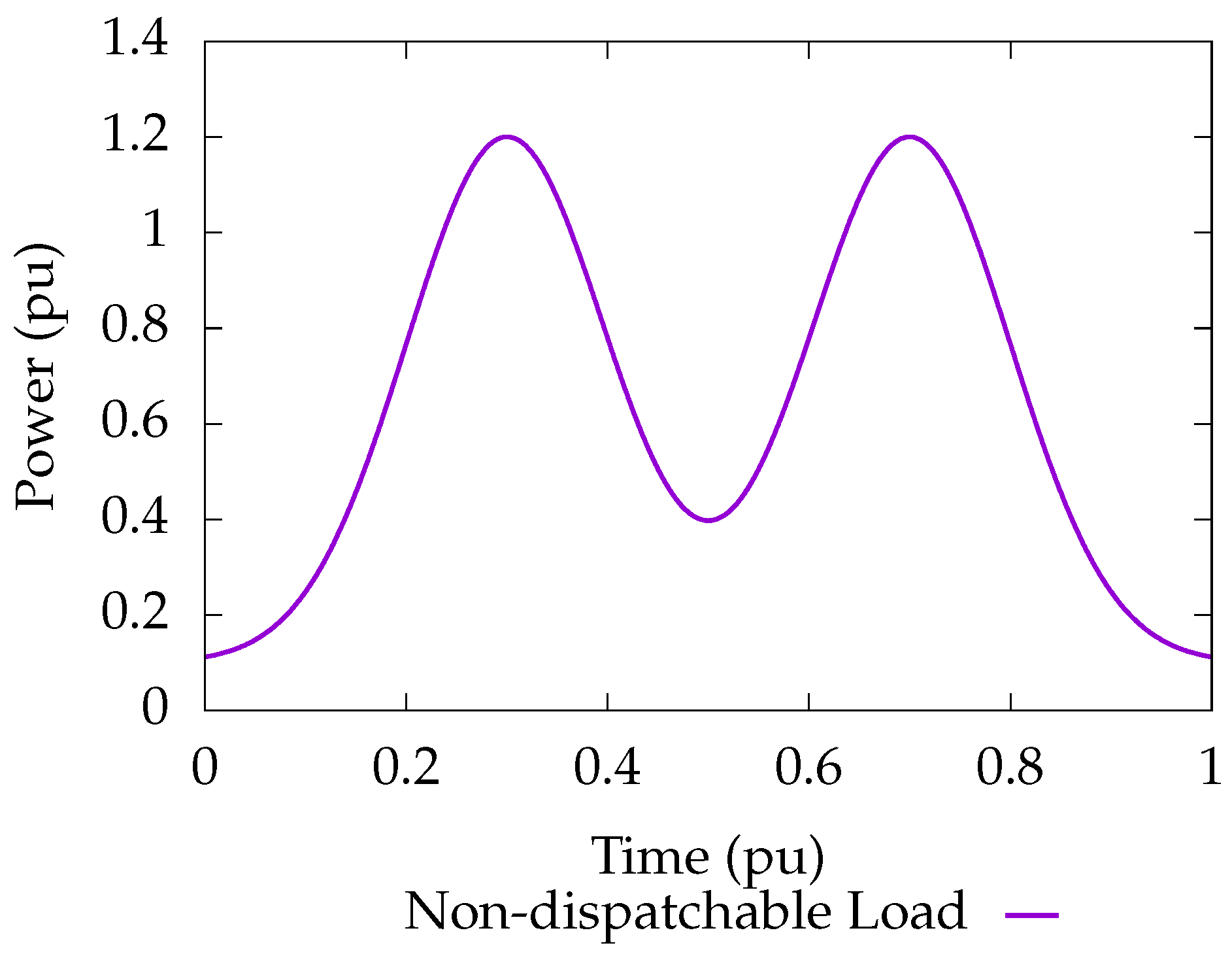
In short, the dynamics in Figure 4 parameterized by Table 7 represent a simple dc generator connected to a dc load. The non-dispatchable load, P, extracts a set amount of power regardless of the voltage level and is given by the two pulses in Figure 5. At maximum, this load consumes 120% of the generation capacity and at minimum it consumes 10%. There are also two resistive loads, one on the generator and one on the load, and each consumes 10% of the generation capacity. In combination, there are points where the demand for power exceeds the generation capacity by 40%. As a result, energy storage is required and provided by the controlled current source, u. Then, the overall amount storage capacity required by this scenario is the difference between the maximum and minimum values in w.

6.2. Discretization

Although the algorithm in this paper and pyomo.DAE use different discretizations, both implement a collocation method and therefore the number of elements and collocation points were set to the same values, 50 and 10, respectively. By default, however, each algorithm uses a different form for the controls. In order to match the algorithms and produce a control that varies less quickly than the state, a piecewise continuous cubic spline based on Bernstein polynomials is used in both codes. Recall, the purpose in generating a control at a coarser time fidelity than the state is to create a formulation where the state can be fully resolved.

6.3. Bounds

In order to limit the amount of generation, a bound on the current coming from the generator is enforced. Since the model assumes a constant voltage on the generator, this inherently limits the amount of power coming from the generator to 1 $\mathrm{pu}$. On the load, the voltage is bounded so that it does not vary more than 10% from its nominal value. Then, as before, each algorithm discretizes the bounds in a slightly different manner. In the algorithm presented in this paper, the coefficients of the polynomials used in the discretization are bounded in such a way where the entire state is bounded over the whole domain. In pyomo.DAE, the states are bounded at the collocation points.

6.4. Objective

In order to determine how much energy storage is required for this particular scenario, the minimization of the norm-square of the amount of energy in the energy storage device, w, is desired. As with the state variables, the discretization of the objective occurs slightly differently between the codes. The algorithm presented in this paper discretizes the desired objective directly so that norm-squared of the amount of energy in the energy storage device is minimized. In pyomo.DAE, the norm-squared of the amount of energy evaluated at the collocation points is minimized.

6.5. Controls

The controls produced by the algorithm in this paper and that of pyomo.DAE are nearly identical and can be seen in Figure 6. This gives some confidence that the control produced by each algorithm represents the optimal control for this particular setup.

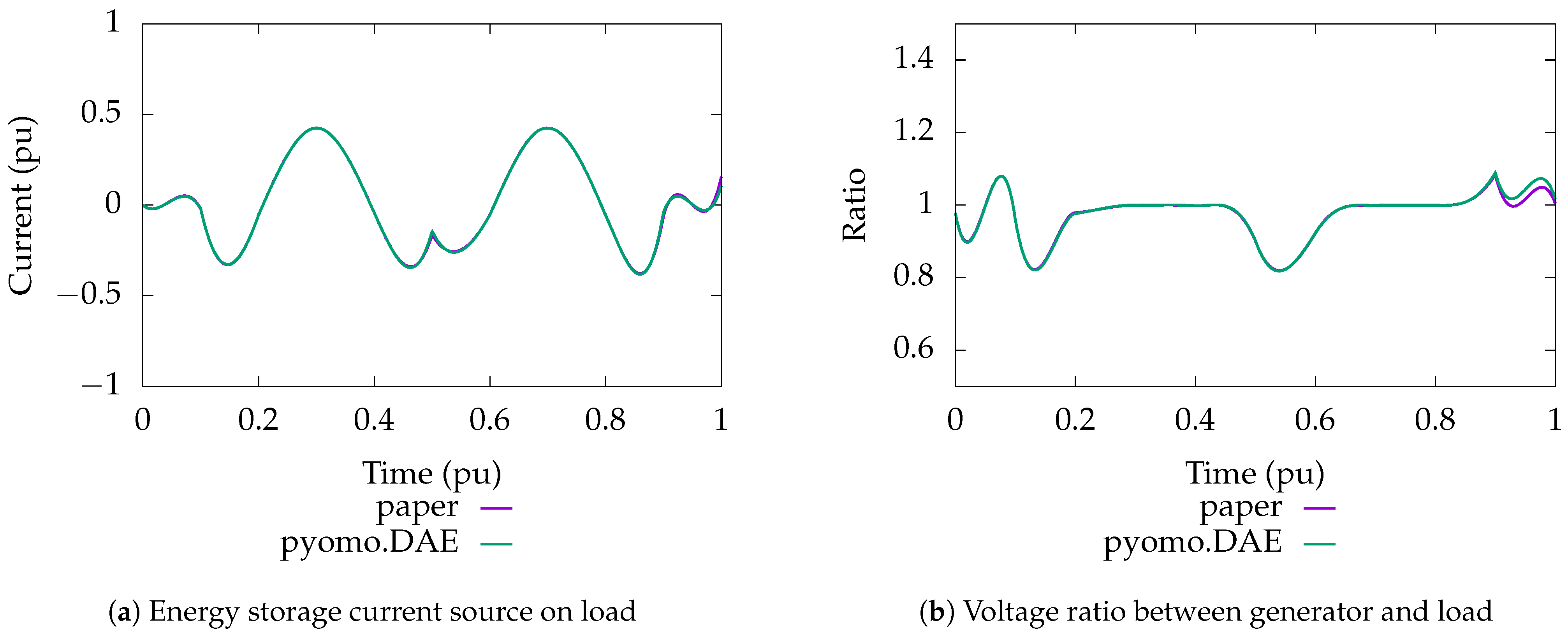
6.6. States

The current and voltage produced by the above controls can be seen in Figure 7. As with the controls, they are nearly identical. That said, there are some minor differences. The maximum current produced by the algorithm in this paper is 9.9999 × 10⁻¹ and the voltage is bounded by [9.0001 × 10⁻¹, 1.0989e], which is inside the specified bounds. In pyomo.DAE, the maximum current produced is 1.0005 and the voltage is bounded by [8.9995 × 10⁻¹, 1.1005], which occur just outside of the specified bounds. Realistically, the amount of bound violation is very small, so this likely does not matter in practice, but one should be aware of the possibility.

6.7. Energy Storage

The amount of energy in the energy storage device as well as the amount of power it stores/produces can be seen in Figure 8. Note, the sign convention used here is that positive power represents storing energy and negative power represents releasing energy. In both cases, the results from this paper and that from pyomo.DAE are nearly identical. The reason that the control stores energy prior to the pulse in power is that objective function attempts to minimize the norm of the amount of energy in the energy storage device. This means the optimal solution tends to split the difference between the amount of energy stored and spent in order to minimize the magnitude of any outliers. As a result, the overall amount of energy storage required for this scenario can be computed by finding the difference between the maximum and minimize values in the amount of energy storage in the energy storage device. For this algorithm, the amount of storage required is computed to be 4.5626 × 10⁻² and for pyomo.DAE this is computed as 4.5605 × 10⁻². While very close, pyomo.DAE is slightly better. Whether this is due to differences in the algorithm or the mild violation of the state bounds is not immediately clear.

6.8. Summary

In short, the algorithm in this paper and pyomo.DAE produce nearly identical controls. Further, the performance of both of these controls is verified using a separate simulation provided by Chebfun, thus avoiding an inverse crime. This gives some confidence that the algorithm described in this paper produces a valid optimal control as described.

It is important to note that the above experiment is not intended to compare the algorithms between this paper and pyomo.DAE. Rather, its intention is to verify that the algorithms in this paper produce a solution in agreement with existing tools, which it does. A more comprehensive study should consider whether the difference in discretization matters to the solution quality and scaling of the algorithm to larger grids. It should also consider the impact of the underlying optimization algorithm used to produce the control. Finally, as the grids become more complicated, one should consider whether a specialized interface to design the grid is preferable to a generic tool.

7. Computational Study

In order to validate the efficacy of this approach, consider a small 9-bus grid based on the Western System Coordinating Council (WSCC) 9-bus test case described by Dembart, Erisman, Cate, Epton, and Dommel in [30]. The parameters used here differ from those in the above paper and are designed to study a mix of turbine and intermittent generation. Specifically, the test here is meant to study the impact of energy storage on the behavior of the grid when a intermittent generation source constitutes a sizable fraction of the generation capacity.

7.1. Description

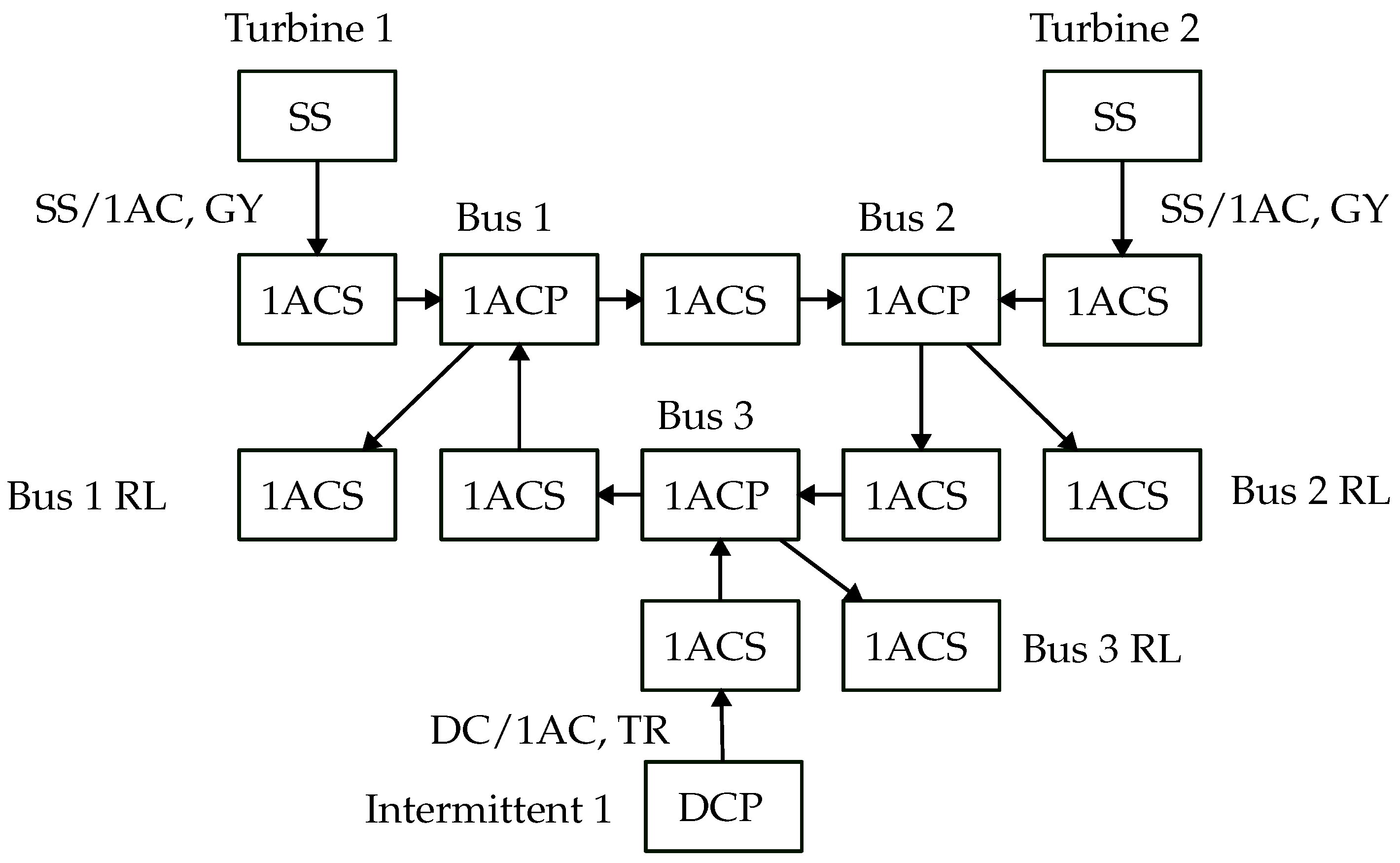
The topology of the grid can be seen in Figure 9 and the parameters that define this grid can be found in

Table 8. Parameters for the nine-bus system described by Figure 9.

Turbine torque, ${\mathit{\tau }}_{\mathit{src}}$	Variable Nm
	$P_{\mathit{src}}\in [0,1]\mathrm{M}\mathrm{W}$
Turbine friction, B	0.140 $\mathrm{N}$,
	2% of 1 $\mathrm{M}\mathrm{W}$ at 60 $\mathrm{Hz}$
Turbine mass moment, J	0.0011 $\mathrm{k}\mathrm{g}{\mathrm{m}}^2$
Turbine damping, D	1 $\mathrm{N}$
Turbine freq., $\omega$	$\omega \in [59.5,60.5]\mathrm{Hz}$,
	60 ± 0.5 $\mathrm{Hz}$
Turb. motor torq. const., K	1 $\mathrm{N}\mathrm{m}/\mathrm{A}$,
Intermittent generation, $i_{\mathit{src}}$	Variable $\mathrm{A}$,
	Generated using SAM using
	1 $\mathrm{M}\mathrm{W}$ dc nameplate
	capacity
Intermittent voltage, $v_{\mathit{src}}$	$v\in [475,525] \mathrm{V}$
Intermittent resist., R	100 $\Omega$
	2.5 $\mathrm{k}\mathrm{W}$ at 500 $\mathrm{V}$
Intermittent capac., C	0.001 $\mathrm{F}$
Turb/inter to bus resist., R	4.11 $\Omega$
	50 $\mathrm{mi}$ of 4/0 AWG
	6/1 AL/STL ACSR
Turb/inter to bus induct., L	0.0128 $\mathrm{H}$
	50 $\mathrm{mi}$ of 4/0 AWG
	6/1 AL/STL ACSR
Turb/inter to bus trans. react. pow., Q	[−200, 200] $\mathrm{k}\mathrm{W}$
Turb/inter to bus stor. react. pow., Q	[−200, 200] $\mathrm{k}\mathrm{W}$
Bus voltage, v	$v\in [\mathrm{15,200},\mathrm{16,800}]\mathrm{V}$,
	16,000 $\mathrm{V}$ ± 5%
Bus resist., R	92,416 $\Omega$
	2.5 $\mathrm{k}\mathrm{W}$ at 15,200 $\mathrm{V}$
Bus capac., C	2 × 10−6 $\mathrm{F}$
Bus RL resist., R	92,416 $\Omega$
	2.5 $\mathrm{k}\mathrm{W}$ at 15,200 $\mathrm{V}$
Bus RL induct., L	2 × 10−6 $\mathrm{H}$
Bus stor. react. pow., Q	[−200, 200] $\mathrm{k}\mathrm{W}$
Bus to bus resist., R	4.11 $\Omega$
	50 $\mathrm{mi}$ of 4/0 AWG
	6/1 AL/STL ACSR
Bus to bus induct., L	0.0128 $\mathrm{H}$
	50 $\mathrm{mi}$ of 4/0 AWG
	6/1 AL/STL ACSR
State var. disc. order	3
State var. disc. mesh	96 elements
Control var. disc. order	3
Control var. disc. mesh	24 elements
Objective	Min. energy squared in energy storage devices (weighted 1)
	Min. difference squared between power generated by turbines (weighted 1 × 10−4)

. Of note, the grid contains two turbine generators with a maximum generation capacity of 1 $\mathrm{M}\mathrm{W}$ and a single solar generator with a maximum nameplate capacity of 1 $\mathrm{M}\mathrm{W}$. The generation profile for the solar generator was produced by the System Advisor Model (SAM) by NREL [31] and is based on estimated generation in Albuquerque, NM in early September. It covers a 24 h period that starts and ends at 12:30 p.m. Note, in order to simplify the succeeding plots, 12:30 p.m. is labeled as hour 0 and other labels designate the number of hours since 12:30 p.m. Hence, hour 8 denotes 8:30 p.m. The load profiles follow a so-called duck curve [32] and are artificially generated. In a duck curve, there is an increase in load after work and again morning prior to work. Note, both the estimate in the amount of solar generation as well as the load profiles are estimates and actual generation and load would likely differ. As a result, a more complete implementation requires an additional feedback controller to help control the difference between the prediction and reality. While important, such a feedback controller requires a more complete discussion and is beyond the scope of this experiment. Finally, energy storage resides in six locations, three on the buses and three on the transmission line between the generators and the buses. All other parameters can be found in Table 8. Note, in order to enhance the performance of the solve, each of these parameters are transformed into per-unit form prior to solve using the methodology in Section 2.

In order to produce a set of initial conditions, the model is first solved using constant elements. Since the derivative of a constant is zero, this produces a steady state solution. Then, this steady state solution is used as the initial condition for the study. Alternatively, the initial conditions could be taken from experimental data or a different kind of steady state solver.

7.2. Controls

A list of the solved control variables can be found in

Table 9. Control variables for the nine-bus system described by Figure 9.

Turbine torque,	${\mathit{\tau }}_{\mathit{src}}$
Voltage ratio on transformer connected to line,	$\lambda$
Phase of transformer connected to intermittent,	$\theta$
Energy storage current/voltage source,	u

. All other variables in the formulation are state variables.

7.3. Bounds

In order to limit the amount of generation from the spinning machines, both the torque and frequency of the turbine are bounded. For the frequency, the model uses a tighter bound of 60 $\mathrm{Hz}$ nominal with $\pm 0.5$ $\mathrm{Hz}$. The bound on the torque is then set to limit the overall amount of generation to 1 $\mathrm{M}\mathrm{W}$. Next, the various bus voltages are limited to vary no more than $\pm 5\%$ from their nominal values.

Finally, the reactive power is bounded throughout the system to be no more than 200 $\mathrm{k}\mathrm{W}$. This occurs at each of the six energy storage devices as well as at the transformers that connect the transmission line to the generation. The purpose of this bound is to improve the power factor at various points within the grid. Note, although it is possible to bound the power factor directly, this is numerically very difficult to achieve when the amount of generation approaches zero. This occurs, for example, at the energy storage devices when the storage is not used. It also occurs at the transformer connected to the intermittent generation at night. As a result, bounding the reactive power as a proxy to power factor largely achieves the goal of bounding the power factor and is easier to accomplish.

7.4. Objective

For the objective, two different goals are desired. First, the amount of energy in the energy storage devices is minimized. Here, the study allows for both positive and negative energy in the energy storage device. Positive energy means the energy storage device has stored energy beyond its initial charge and negative energy means it has spent it. The peak-to-peak amount of energy indicates the minimum amount of energy required in the energy storage devices to operate the grid given the specified loads and generation profiles. Note, modifying the objective weighting changes where the MPC chooses to use the energy storage. This study considers two different scenarios, one where all of the energy storage is weighted equally and another where the weighting on energy storage on the bus closest to the intermittent generation is half that of the others. Second, the difference between the generation of turbines is penalized. This helps to force the MPC to produce a control that uses the turbines equally. Since this objective is mostly used for its regularizing effect, its weight is much smaller than its use of the energy storage.

7.5. Solver

The resulting optimization formulation is solved using a prototype version of Optizelle [33]. This algorithm implements a modified version of NITRO [34], which is a kind of composite step SQP algorithm combined with a primal-dual interior point method. It differs from NITRO by implementing an augmented Lagrangian merit function as well as mechanisms that allow for inexactness in the linear system solves in a manner similar to the algorithm developed by Ridzal and Heinkenschloss [35,36,37]. The linear systems within the algorithm are solved using a rank-revealing QR factorization devised by Davis [38]. Overall, the formulation contains 36,864 variables, 19,662 equations, and 16,320 bounds. All metrics for optimality were solved to an error 1 × 10⁻⁸.

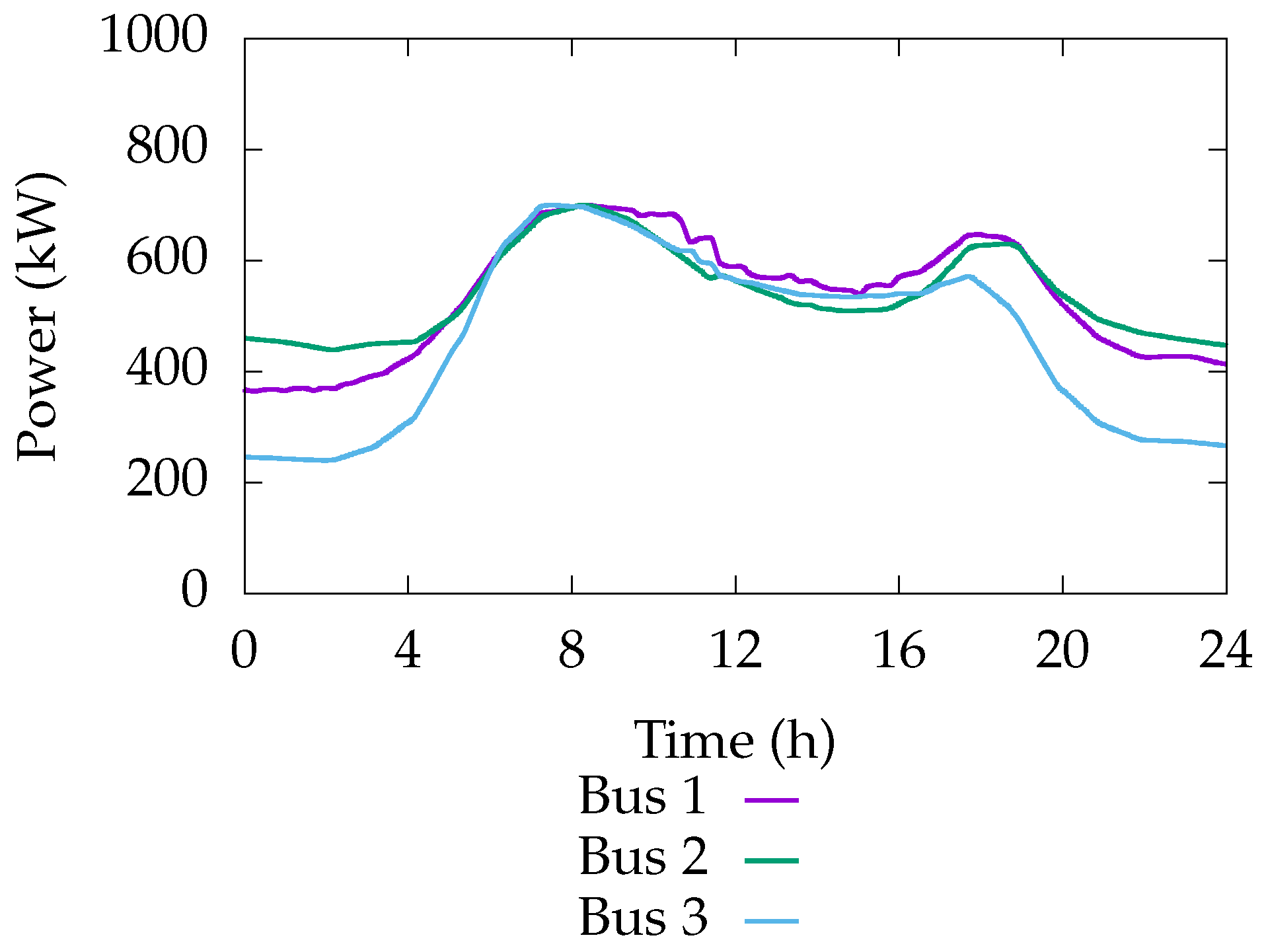
7.6. Load

The load profile can be found in Figure 10 and has a maximum power of 700 $\mathrm{k}\mathrm{W}$. Recall, it follows a duck curve that has been rotated to start at 12:30 p.m. In this curve, there are two spikes in load. The first occurs around hours 5–9, which correspond to 5:30 p.m.–9:30 p.m. and indicate an increase in power usage when families return home from work. The second occurs around hours 17–20, which correspond to 5:30 a.m.–8:30 a.m. and indicate an increase in power usage when families wake up in the morning.

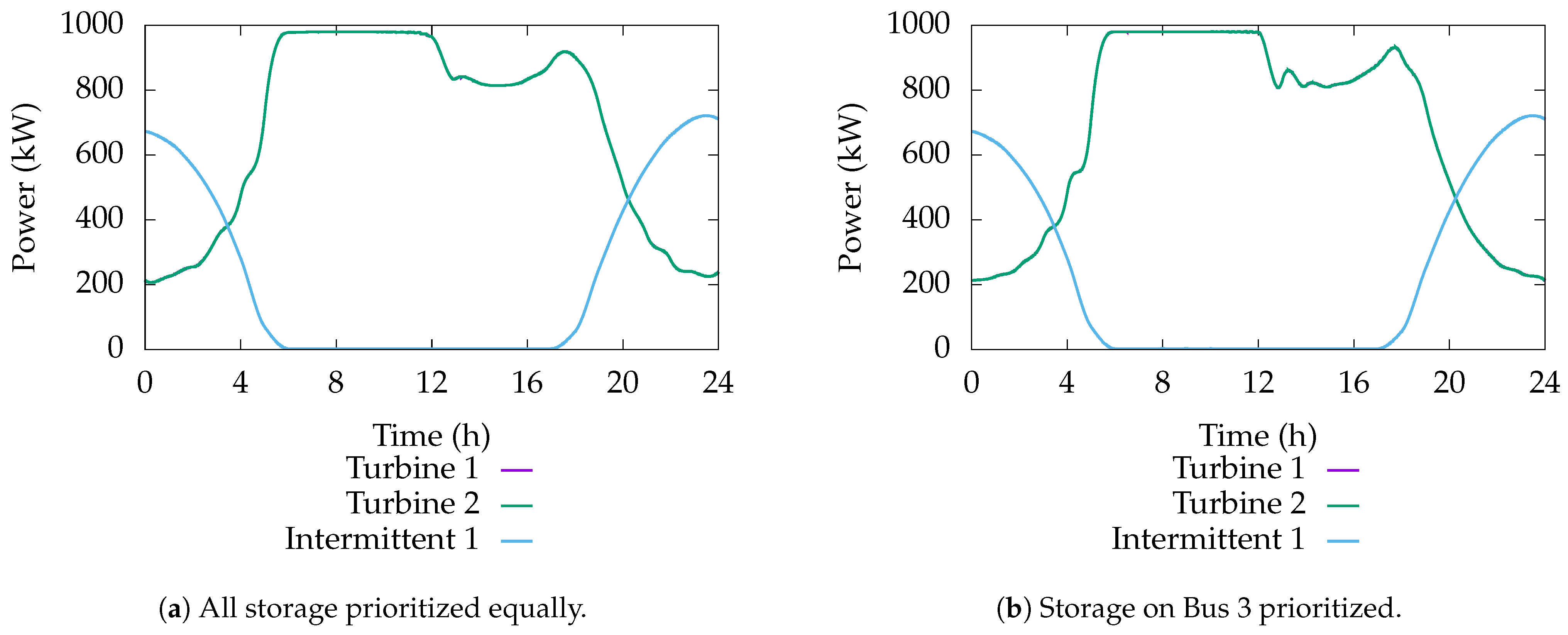
7.7. Generation

The generation can be found in Figure 11. Here, it can be seen that the solar generation drops off at night whereupon the turbine generation compensates. The reactive power due to generation can be seen in Figure 12. In this plot, the reactive power is very low compared to the active, so the power factor is close to 1 as long as there is generation. This is notably very high and results from the optimal control explicitly bounding the reactive power at the energy storage devices as well as the connection between the generators and the buses. At night, the power factor on the solar generation is highly variable, but its apparent power is near zero. Note, the amount of power generated by the turbines is largely driven by the controlled torque, which can be found in Figure 13. The shape of this parameter closely matches the active power.

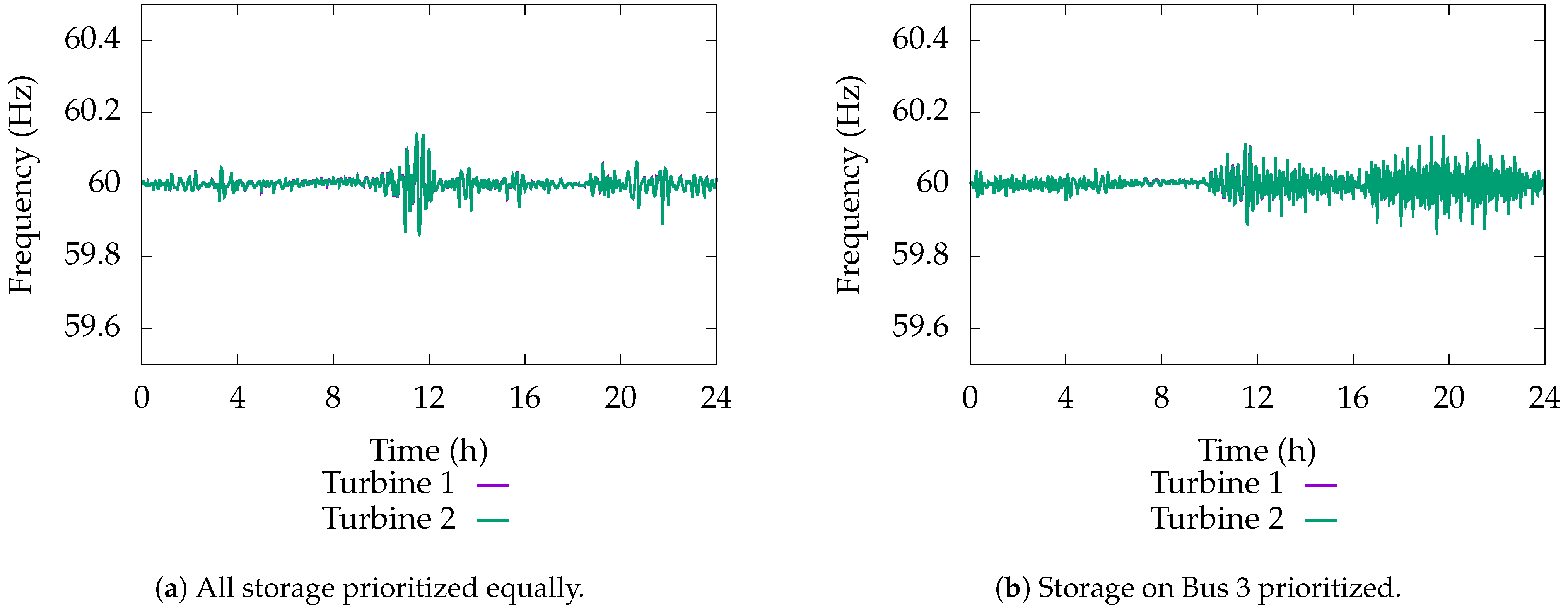
7.8. Turbine Frequency

The frequency of the turbines can be seen in Figure 14. Note that the frequency lies near the nominal 60 $\mathrm{Hz}$.

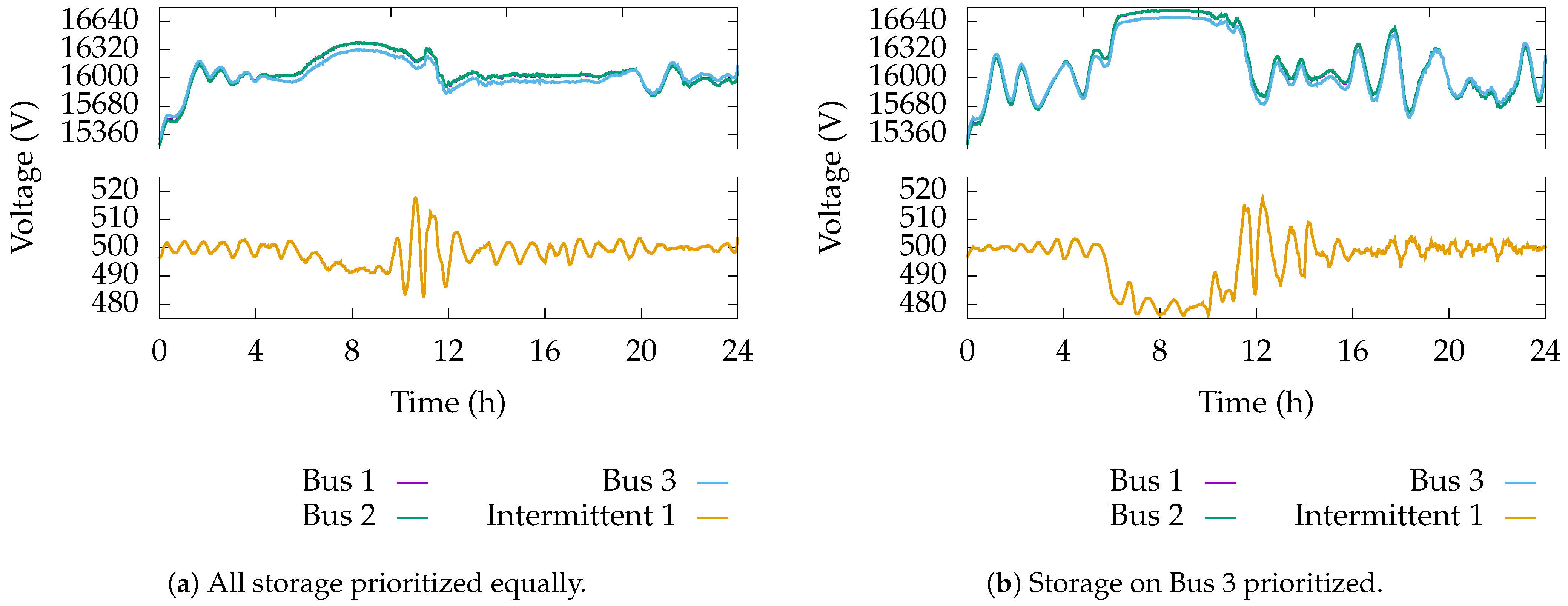
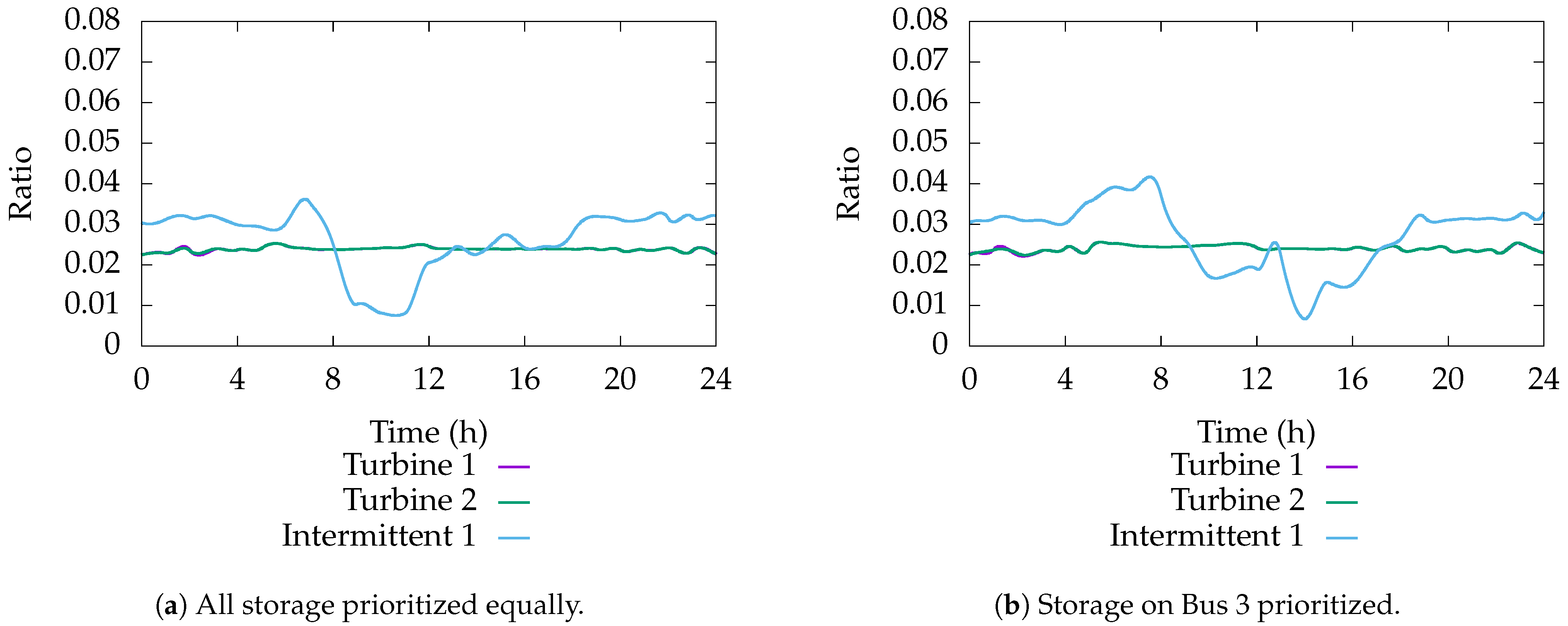
7.9. Bus Voltages

As far as the voltages on the grid, they can be seen in Figure 15. Each lies within the specified 5% of their nominal value. The voltage ratio on the transformers that help maintain these voltages can be found in Figure 16.

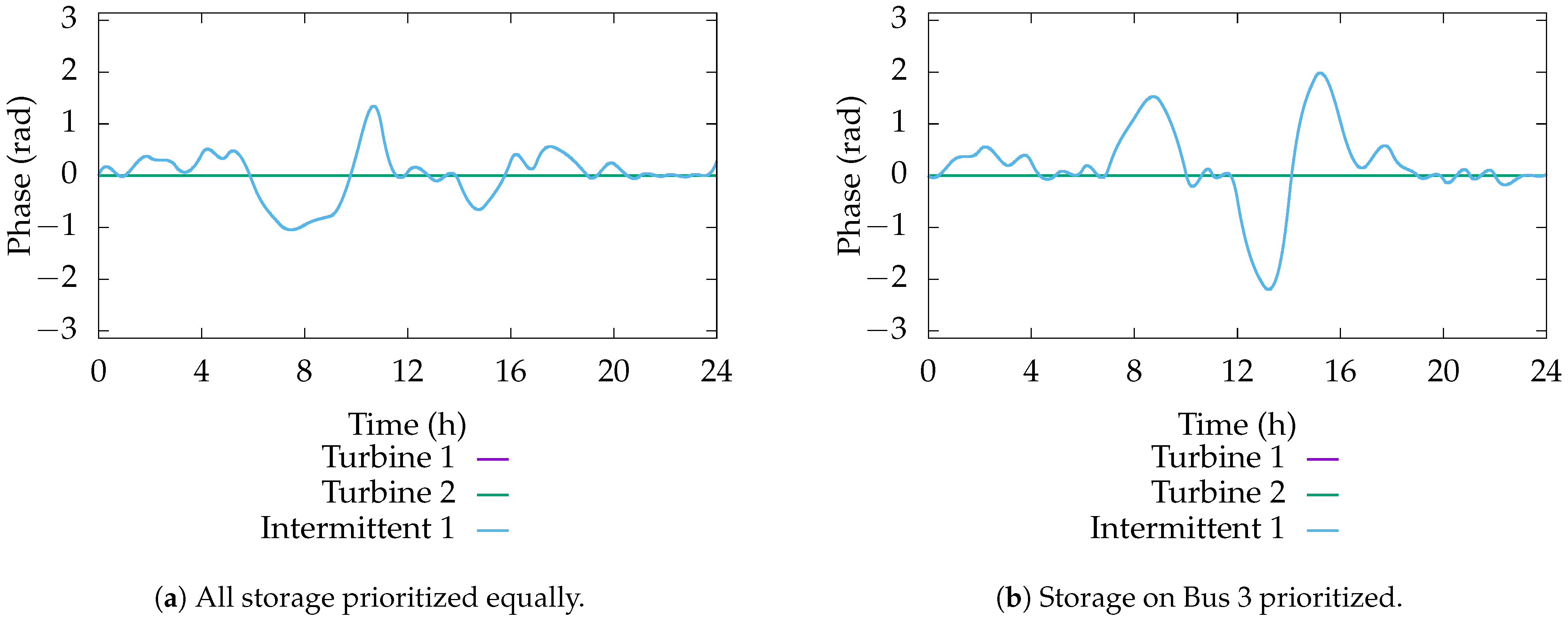
7.10. Transformer Phase

The phase of the transformers can be seen in Figure 17. Note, since Turbine 1 represents the reference machine, the phase on its transformer is set to 0. The phase on Turbine 2 is a state variable related to the difference in frequencies and it largely matches Turbine 1. Then, the phase on the transformer connected to Intermittent 1 is actively controlled. Between the two, there is far more variation on the actively controlled phase on the transformer connected to Intermittent 1. Beyond the overall metrics for optimality, it is not yet known why the MPC found this variation most beneficial.

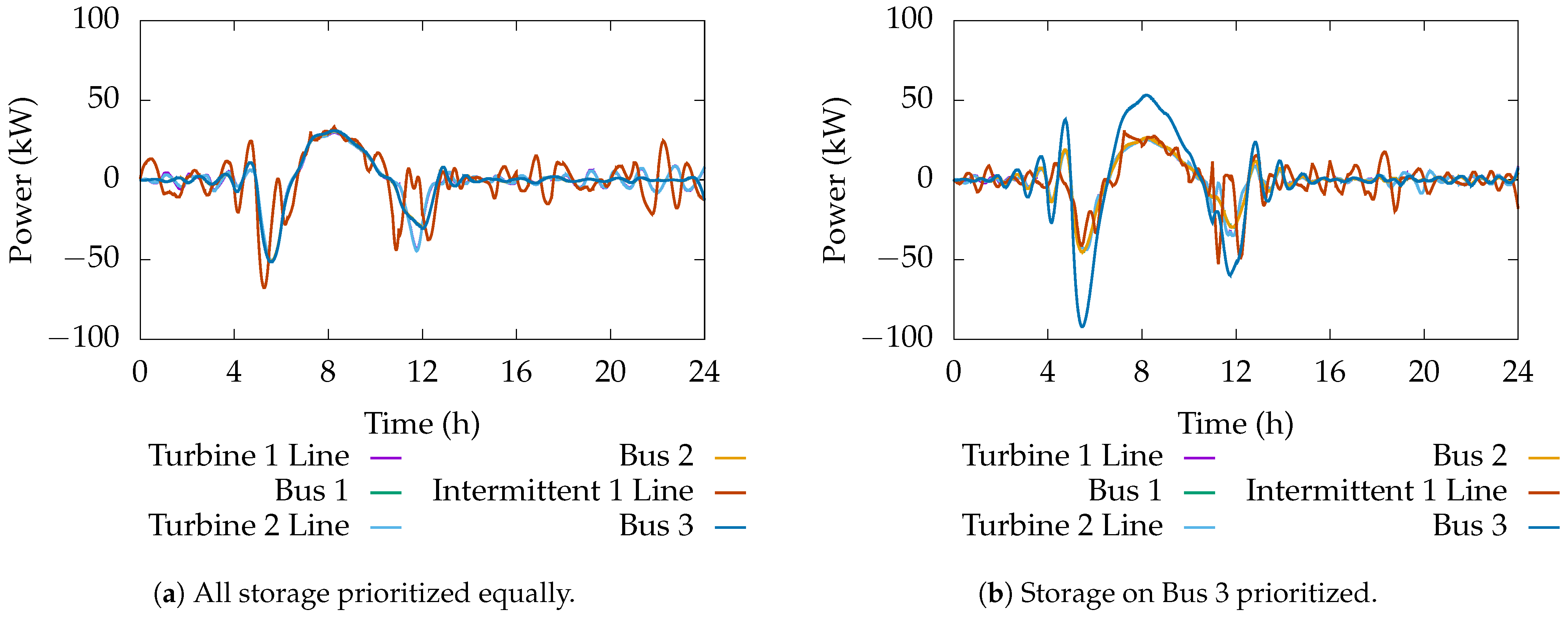
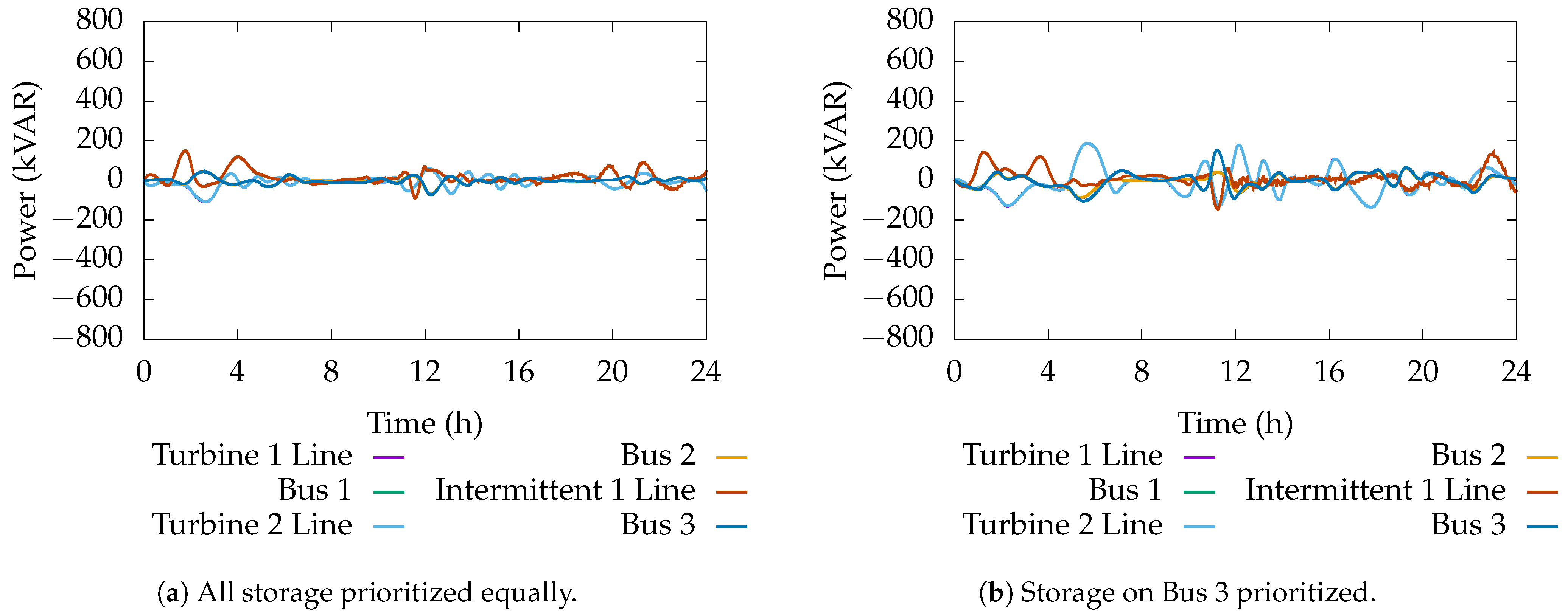
7.11. Energy Storage

Finally, the active and reactive power from the energy storage devices can be seen in Figure 18 and Figure 19, respectively. Here, the amount of reactive power remains bounded and small, as specified in the formulation. Active power is stored just prior to the spike in load during the evening, used over this period, and then recharged when the load subsides. The reason the two spikes in energy storage occur is that the MPC minimizes the amount of energy in the energy storage device squared. This tends to minimize outliers, which inherently limits storing too much power or expending too much power. Essentially, the MPC splits the difference between the two, which results in a store-use-store pattern. In the case where the MPC penalized the use of energy storage on Bus 3 less than the other storage devices, the MPC prioritized its use of that energy storage device more. This is expected and demonstrates how changing the objective weights changes the behavior of the control. Finally, the amount of energy in the energy storage device can be seen in Figure 20. Recall, the MPC set the nominal value for energy to be 0 $\mathrm{k}\mathrm{W}\mathrm{h}$. This means that positive energy corresponds to energy storage and negative energy corresponds to energy delivery. As a result, the peak-to-peak values indicate the overall amount of energy storage required for this particular scenario. This value may be useful during the design process for determining the amount of energy storage needed on the grid (design specifications and requirements utilized in sizing energy storage devices).

7.12. Summary

In short, the MPC produces a control that operates the grid in a well-performing manner. The amount of reactive power is low; the overall power factor is high; and, the energy storage is used efficiently. Further, the study shows how reweighting the objective function can change the behavior of the grid.

8. Conclusions

The preceding article described an MPC well-suited for the resilient integration of intermittent resources into the power grid. It developed a ROM that provides more detail than a power flow model, but less than an EMT model, carefully tailored for integration into an MPC. This process involved developing a series of abstractions that allows a grid to be quickly assembled from a combination of dc, 3-phase ac, steady state 1-phase ac, and spinning machine components. In addition to the ROM, a modified per-unit transformation was presented that integrates well into these abstractions. Next, the optimization formulation for the MPC was presented. This discussion explained why a full-space formulation is desirable for this kind of MPC and it gave a collection of objective functions that can tune and modify the behavior of the control. Following this discussion was a presentation of the discretization used by the MPC. Here, an OSC method based on Bernstein polynomials was presented. This discussion advocated for the use of Bernstein polynomials since the state and control variables, and their higher order derivatives, could be bounded over the entire domain. In addition, a scaling method was presented that transformed the method, so that the ${\ell }^2$-norm of the state and control variables as well residual of the constraints corresponded to the $L^2$ norm of their functional counterparts. This not only allows the MPC to use most available optimization solvers without explicitly changing the inner product, but it allows for greater ease during mesh refinement since the norm of the variables remains roughly the same. Next, the paper presented a set of strategies for refining the behavior the MPC. Since every solution to the MPC can be considered optimal, understanding how to tune the behavior the MPC is critical to its performance.

The algorithm was then validated using two separate numerical studies. In the first, the algorithm in this paper was compared to a result generated from pyomo.DAE. Then, the controls generated from both codes were passed to a high-precision simulation computed by Chebfun. From this experiment, it was seen that both controls were nearly identical, which means the MPC produces a solution in agreement with existing tools. The high-precision simulation validates that states were controlled as desired. In the second experiment, a computation study was conducted on a modified version of the WSCC 9-bus test case. Here, it was seen that the MPC allowed for a study of a grid with a high penetration of intermittent resources. Such grids require energy storage to operate and the MPC was able to assess the impact of its location and amount for one such scenario. This study helps to validate that the methodology and framework presented in this article can be usefully applied to the control and design of grids with intermittent energy resources.

As far as future work, additional grid topologies and scenarios should be investigated. This would likely lead to the development of additional power system abstractions, which would improve the utility of the MPC as a tool for both control as well as the design of future grids. In addition, the integration of the MPC with a feedback controller to track the MPC solution should also be investigated. Since the MPC produces a time-dependent control, the stability analysis in a feedback control requires careful consideration. Finally, a more thorough investigation of economic aspects and cost-effectiveness may lead to insightful uses in resource planning. Such features may be readily introduced through the objective function.