A Semi-Analytical Model for Pressure Transient Analysis of Multiple Fractured Horizontal Wells in Irregular Heterogeneous Reservoirs

Abstract

The irregular outer boundaries of reservoirs and the associated heterogeneous high-permeability zones formed by complex geological environment pose significant challenges in reservoir characterization and performance prediction. These irregular geometries, which are commonly encountered in field applications but often oversimplified in conventional models, can substantially influence fluid flow dynamics and transient pressure behavior. To solve this critical issue, this paper presents a semi-analytical model for studying the transient pressure behavior of irregular heterogeneous reservoirs, focusing on the dynamic interactions between hydraulic fractures and the surrounding matrix. The model integrates Green’s function solutions for matrix flow with finite difference methods to simulate fluid flow within complex fracture networks, capturing the heterogeneity of the reservoir and the irregularity of its boundaries. Specifically, the reservoir is divided into locally homogeneous blocks, and the flow within each block is solved using bounded Green’s functions, while the fracture networks are discretized and solved using finite difference methods. This proposed model significantly reduces computational complexity compared to traditional numerical simulations, while maintaining high accuracy. Subsequently, we conducted comprehensive parameter sensitivity analyses. The calculational results show that a multi-fractured horizontal well in an irregular heterogeneous reservoir can observe the following flow regimes: bilinear flow, elliptical flow, and boundary-dominated flow. Longer fractures and higher conductivity enhance fracture flux by increasing the contact area and reducing flow resistance, respectively. However, these positive impacts are constrained by drainage area limitations as production progresses.

1. Introduction

The development of unconventional reservoirs, such as tight oil and shale gas, has become increasingly important in meeting global energy demands [1]. Hydraulic fracturing is a key technology for enhancing the productivity of these reservoirs by creating complex fracture networks that serve as conduits for fluid flow [2]. However, reservoir heterogeneity and complex geological structures introduce significant challenges in accurately predicting well performance. Existing modeling approaches often simplify these complexities, leading to inaccurate estimations in pressure transient analyses and production forecasts [3,4]. Therefore, there is a critical need for advanced modeling techniques that can more effectively capture the effects of reservoir heterogeneity and irregular geometries to improve well performance predictions and optimize hydraulic fracturing designs.

Current methods for modeling fluid flow in reservoirs can be broadly categorized into numerical, analytical, and semi-analytical approaches [5]. Numerical methods, such as finite difference and finite element approaches, are widely used for simulating fluid flow in heterogeneous reservoirs due to their ability to handle complex geometries and boundary conditions [6,7]. For example, Correia et al. [8] integrated geostatistical modeling of carbonate reservoir heterogeneities, such as fractures and vugs, with upscaling and flow simulation, offering a dual permeability approach to better model flow in both matrix and fractured regions. Li et al. [9] proposed a simulated reservoir model using the embedded discrete fracture method (EDFM) to simulate multiphase flow in heterogeneous reservoirs with complex fractures, highlighting the importance of considering heterogeneity and fracture effects in injection and production processes. Khadivi [10] introduced a new numerical well test procedure using the finite element method and zonal discretization, improving the accuracy of detecting interior boundaries and quantifying permeability heterogeneity in radially heterogeneous reservoirs. Luo et al. [11] explored the impact of heterogeneous porosity and permeability on carbon dioxide (CO₂)-enhanced oil recovery (EOR) in tight reservoirs, revealing that increased heterogeneity leads to flow channeling, reduced oil production, and lower CO₂ storage. Zhang et al. [12] developed 3D coupled Thermo–Hydro–Mechanical (THM) reservoir models to evaluate the impact of fracture and stimulated reservoir volume (SRV) permeability heterogeneity on heat extraction, focusing on different stress conditions to better understand geothermal reservoir performance. However, these numerical models often require extensive computational resources and fine grid discretization, making them time-consuming and less practical for large-scale or real-time applications. Analytical solutions, on the other hand, provide efficient and precise results for idealized reservoir conditions but struggle to accommodate irregular boundaries and intricate fracture networks [13,14].

Semi-analytical methods serve as an intermediate solution, balancing computational efficiency with the ability to incorporate more complex reservoir characteristics. These methods are particularly well-suited for modeling transient pressure behavior in reservoirs with irregular boundaries and heterogeneous fractured zones, providing a balance between accuracy and computational efficiency. For example, Shi et al. [15] developed a semi-analytical proxy for modeling solvent transport in Vapex, enabling efficient assessment of reservoir heterogeneity and optimization of production with lower computational costs. Cheng et al. [16] introduced a hybrid method for modeling fluid flow in fractured heterogeneous reservoirs, combining Green-function solutions, dual porosity models, and finite element analysis for efficient and accurate simulation of fractured horizontal wells. Tian et al. [17] presented a semi-analytical model for multi-wing fractured vertical wells in heterogeneous gas reservoirs, addressing nonlinearities and evaluating the impact of crossflow, fracture conductivity, and reservoir size on well performance. Li et al. [18] proposed a semi-analytical model for horizontal wells with complex fracture networks in heterogeneous reservoirs, considering heterogeneity and fracture geometry, and offering insights into pressure behavior and well-test interpretation in tight reservoirs. Ren et al. [19] developed a semi-analytical three-region linear composite model for multi-wing fractured vertical wells in bilaterally heterogeneous gas reservoirs, addressing pressure response and rate decline influenced by well location, fracture properties, and reservoir heterogeneity. Deng et al. [20] presented a semi-analytical model to analyze pressure behavior in heterogeneous, channelized reservoirs with partially communicating faults, highlighting the impact of heterogeneity and fault systems on well performance. It can be seen from these models that recent studies have extended semi-analytical approaches to evaluate solvent transport in Vapex, fluid flow in fractured reservoirs, and pressure responses in composite models. While these models offer valuable insights, most existing research primarily focuses on reservoir heterogeneity, with limited consideration of irregular geometries and complex geological structures. As a result, current semi-analytical models may not fully capture the pressure transient behavior in reservoirs with intricate boundary conditions and fracture geometries.

To address this research gap, this work develops a semi-analytical model to analyze the transient pressure behavior of irregular heterogeneous reservoirs. With the aid of this semi-analytical model, the heterogeneous reservoir is divided into multiple homogeneous subdomains (blocks) with distinct permeability properties, where each block is governed by Green’s function solutions for matrix flow. Fracture networks and inter-block interfaces are discretized into segments using finite difference methods, and pressure/flux continuity conditions are enforced at boundaries. Unlike traditional numerical simulations that require full discretization of the entire reservoir, this approach only discretizes fractures and interfaces, significantly reducing computational complexity. The use of Laplace transforms further enhances efficiency by simplifying the governing equations before numerical inversion. Subsequently, the effects of the permeability heterogeneity, the fracture length, and the fracture conductivity on pressure dynamics are investigated.

2. Methodology

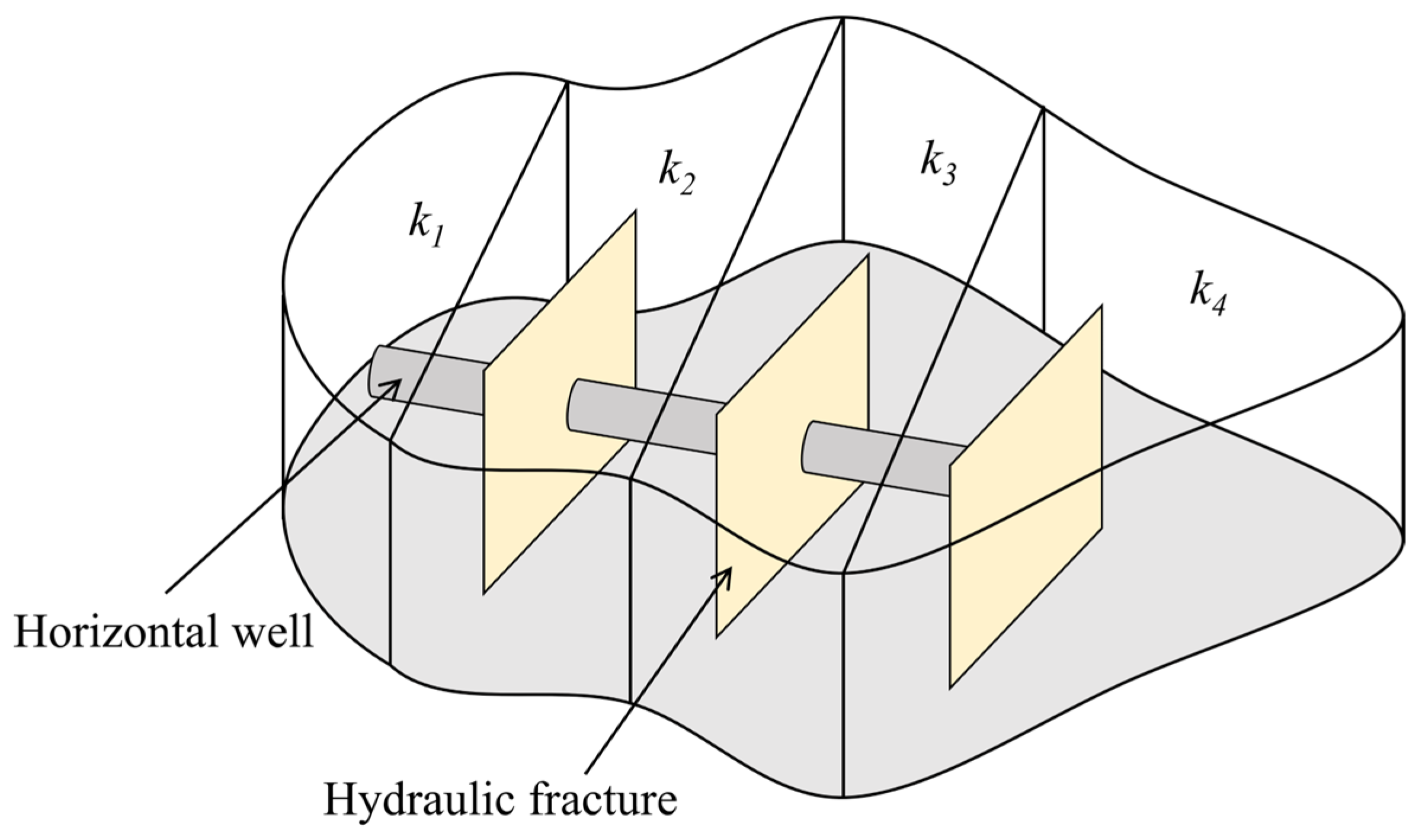
2.1. Physical Model

Figure 1 shows the physical model for a multiple-fractured horizontal well in a heterogenous reservoir with irregular boundary. Subject to a complex sedimentary environment, the reservoir consists of multiple regions with distinct permeability characteristics (e.g., k¹, k², k³, k⁴). The outer boundary of the reservoir is impermeable and exhibits irregular geometry [16,17]. The horizontal well is intersected by multiple hydraulic fractures, which extend into the reservoir and create a complex fracture network. The modeling of multiple-fractured horizontal wells penetrating multi-heterogeneous zones has been widely studied by numerous scholars, demonstrating its relevance in unconventional reservoir development [20]. To construct a semi-analytical model, the following assumptions are given:

(1)

Each region is assumed to be homogeneous with the same layer thickness.

(2)

Because the reservoir is fully penetrated by the hydraulic fractures and the reservoir length is significantly greater than its thickness, the flow pattern can be simplified as a 2D flow.

(3)

The flux distribution along the hydraulic fracture is non-uniform.

(4)

The well flow is produced at a constant rate, and the fluid enters the well only through the hydraulic fracture. It is worth noting that the assumption of a constant production rate is a simplification, as actual production rates often vary due to pressure depletion and operational constraints.

(5)

The flow conductivity of the wellbore is infinite, meaning pressure loss along the wellbore is ignored.

(6)

The effects of gravity and capillary forces are negligible.

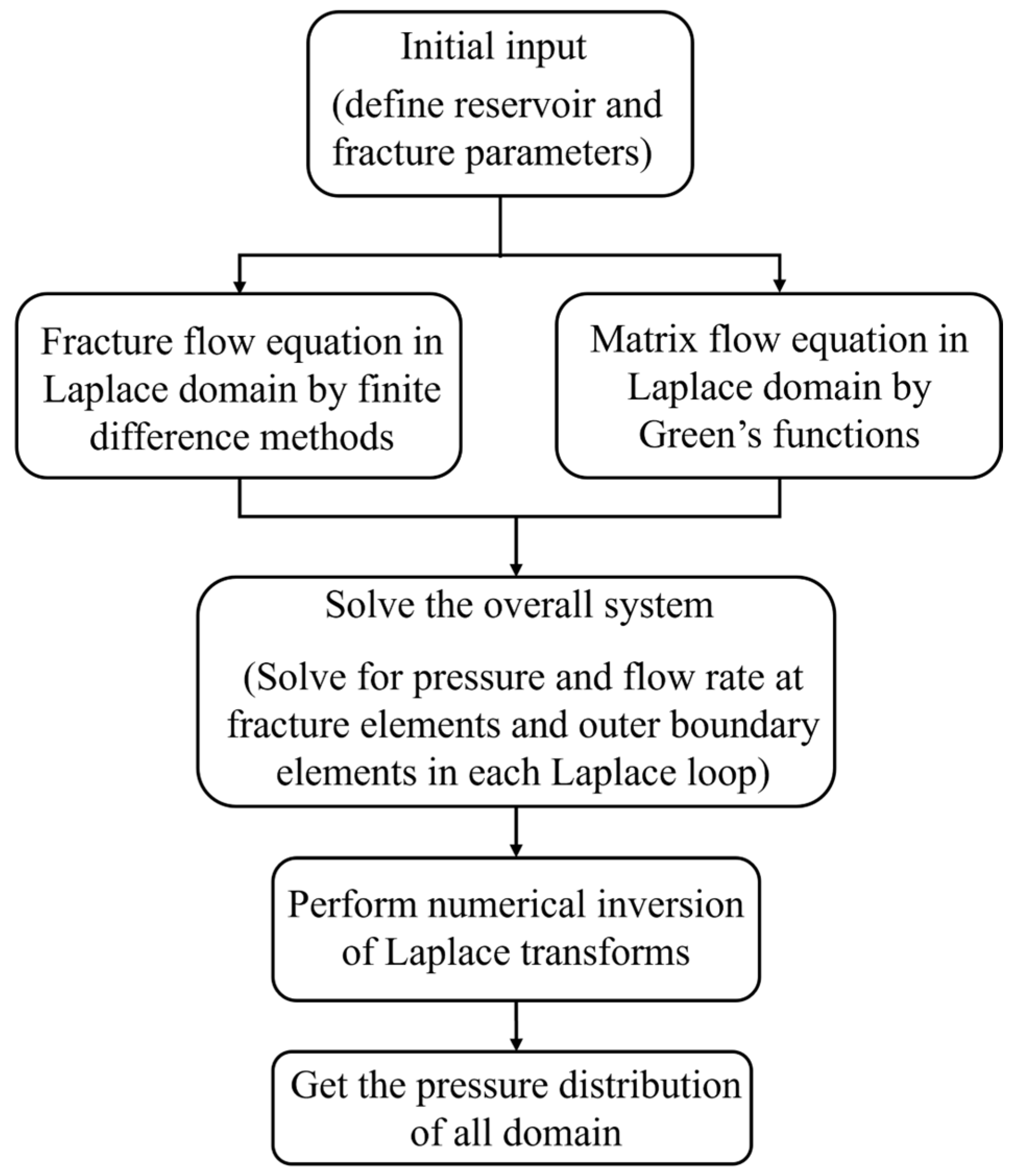
2.2. Mathematical Model

As shown in Figure 2, the whole reservoir is divided into several homogeneous rectangular blocks by the difference of permeability. According to irregular geometric boundaries, the length and width of each individual block can be adjusted. The interfaces between the blocks and fractures within each block can be discretized into segments. Each segment can be regarded as a linear source of a 2D bounded reservoir. For convenience, the following dimensionless variables are defined:

$$p_D={\displaystyle \frac{2\mathsf{\pi }\beta k_{ref}h(p_i-p)}{q_{w}B\mu }}; t_D={\displaystyle \frac{\beta k_{ref}t}{{\varphi }_m\mu c_{tm}{L_f}^2}}; C_s={\displaystyle \frac{{\varphi }_f{c}_{tf}}{{\varphi }_m{c}_{tm}}}; C_{fD}={\displaystyle \frac{k_{f}w}{k_{ref}{L}_f}}$$

(1)

$$q_{fD}={\displaystyle \frac{q_f}{q_w}}; q_{eD}={\displaystyle \frac{q_e}{q_w}}$$

(2)

where P_D is the dimensionless pressure, β is the unit conversion factor with a value of 0.0853, k_ref is the reference matrix permeability, h is the reservoir thickness, P_i is the initial reservoir pressure, q_w is the production rate of oil well, B is the formation volume factor, µ is the oil viscosity, t_D is the dimensionless time, t is the time, ϕ_m is the matrix porosity, c_tm is the matrix total compressibility, L_f is the half facture length, ϕ_f is the fracture porosity, c_tf is the fracture total compressibility, C_fD is the dimensionless fracture conductivity, k_f is the fracture conductivity, w_f is the fracture width, q_fD is the flow rate from the matrix to the fracture, q_e is the flow rate at the interface between the blocks.

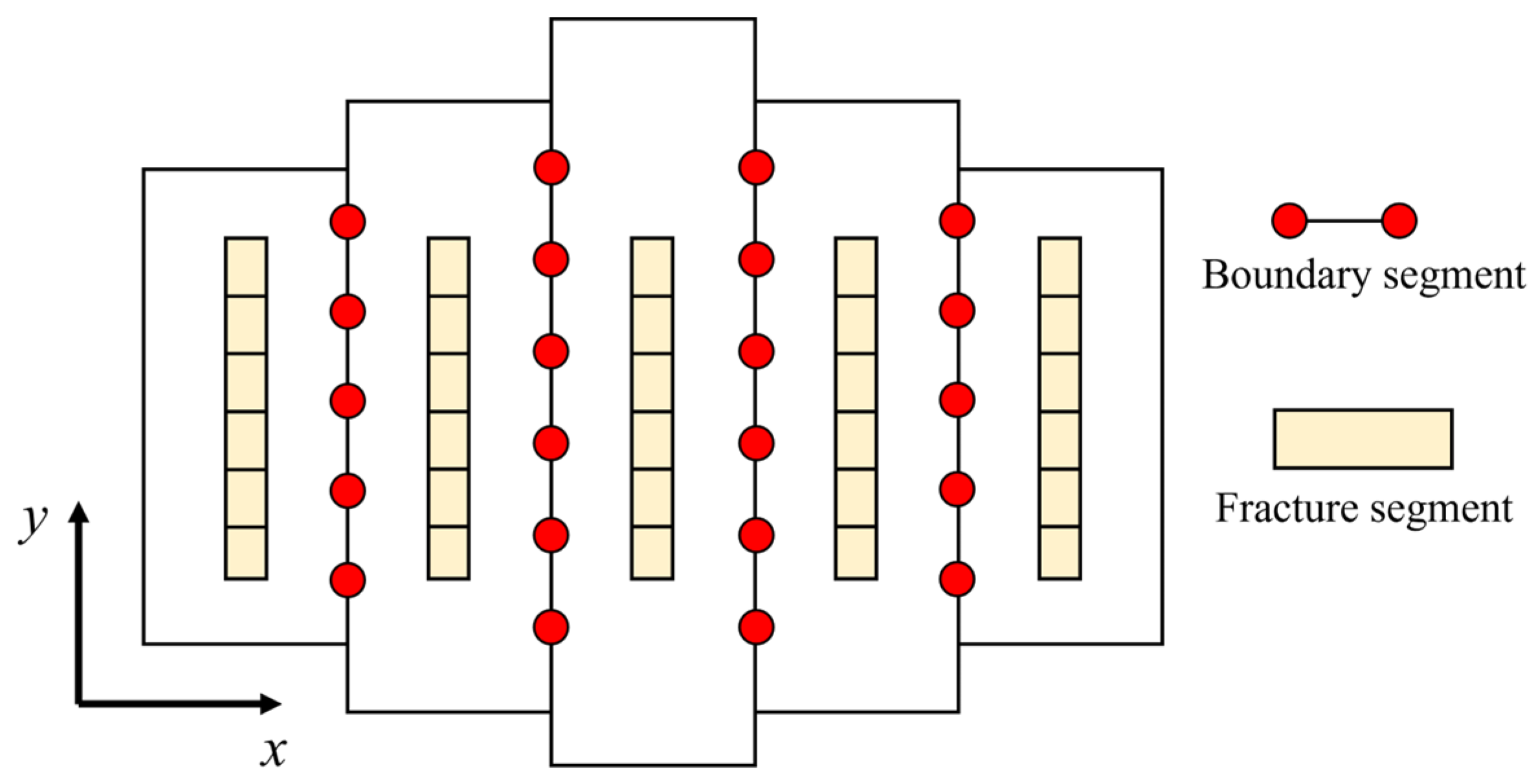
2.2.1. Fluid Flow Within the Fracture System

Based on the aforementioned assumptions and incorporating the principle of material balance, the pressure distribution for a single fracture system can be mathematically formulated in the Laplace domain as follows:

$${\displaystyle \frac{{𝜕}^2{\overline{P}}_{fD}}{𝜕l_{fD}^2}}-{\displaystyle \frac{2\pi {\overline{q}}_{fD}}{\Delta l_{fD}{C}_{fD}}}={\displaystyle \frac{s{C}_s{w}_D}{C_{fD}}}{\overline{P}}_{fD}$$

(3)

where l_fD is the spatial position along the fracture, s is the Laplace parameter, and superscript “−” is the Laplace transform. Applying finite-difference approximation to Equation (3), the discrete formulation for pressure change of ith fracture segment can be written as:

$${\displaystyle \frac{1}{\Delta l_{fD}}}{\overline{P}}_{fDi+1}-\left({\displaystyle \frac{2}{\Delta l_{fD}}}+{\displaystyle \frac{s{C}_s{w}_D}{C_{fD}}}\right){\overline{P}}_{fDi}+{\displaystyle \frac{1}{\Delta l_{fD}}}{\overline{P}}_{fDi-1}-{\displaystyle \frac{2\pi }{\Delta l_f{C}_{fD}}}{\overline{q}}_{fDi}=0$$

(4)

For convenience, the following parameters are defined:

$$a={\displaystyle \frac{1}{\Delta l_f}}, A={\displaystyle \frac{2}{\Delta l_f}}+{\displaystyle \frac{s{C}_s{w}_D}{C_{fD}}}, b={\displaystyle \frac{2\pi }{\Delta l_f{C}_{fD}}}$$

(5)

As such, Equation (4) can be rewritten as:

$$a_{i+1}{\overline{P}}_{fDi+1}-b_i{\overline{P}}_{fDi}+a_{i-1}{\overline{P}}_{fDi-1}-c_i{\overline{q}}_{fDi}=0$$

(6)

By systematically applying Equation (6) to all fracture segments within the discretized system and employing matrix transformation techniques, we derive the matrix representation of the pressure distribution as follows:

$$\mathit{A}\cdot {\overline{\mathit{P}}}_f+\mathit{B}\cdot {\overline{\mathit{q}}}_f+\mathit{C}\cdot {\overline{q}}_{f-w}=\mathit{D}$$

(7)

where A represents an N × N matrix; B, C, and D represent N × 1 matrices; and q_f-wD is the flow rate from the fracture to the production well. They can be expressed as:

$$\mathit{A}=\left[\begin{array}{ccccc}{A}_1& a_2& 0& \dots & 0\\ a_1& A_2& a_3& \ddots & ⋮\\ 0& a_2& A_3& a_4& 0\\ ⋮& \ddots & \ddots & \ddots & \ddots \\ 0& \cdots & 0& a_{N-1}& A_N\end{array}\right], \mathit{B}=\left[\begin{array}{c}b\\ ⋮\\ b\\ ⋮\\ b\end{array}\right], \mathit{C}=\left[\begin{array}{c}0\\ ⋮\\ -b\\ ⋮\\ 0\end{array}\right], \mathit{D}=\left[\begin{array}{c}0\\ ⋮\\ 0\\ ⋮\\ 0\end{array}\right], {\overline{\mathit{P}}}_f=\left[\begin{array}{c}{P}_{fD1}\\ P_{fD2}\\ ⋮\\ ⋮\\ P_{fDN}\end{array}\right], {\overline{\mathit{q}}}_f=\left[\begin{array}{c}{q}_{D1}\\ q_{D2}\\ ⋮\\ ⋮\\ q_{DN}\end{array}\right]$$

(8)

2.2.2. Fluid Flow Within the Matrix System

Since the reservoir is divided into n_b homogeneous blocks, the pressure distribution within the matrix system is derived by taking a single block as an example. For the jth homogeneous block, its transient pressure behavior is governed by the superposition of all contributing linear sources, which include n fracture segments and m interface segments between adjacent blocks. Using the fundamental solution provided by Green’s function and applying the principle of superposition, the analytical solution for the pressure distribution within jth homogeneous block can be expressed as follows:

$${\overline{P}}_D^j\left(x_D,y_D,s\right)=\left[{\displaystyle \sum _{i=1}^n{\overline{q}}_{fDi}^j\cdot G_{fi}^j\left(x_D,y_D,s\right)}\right]+\left[{\displaystyle \sum _{i=1}^m{\overline{q}}_{eDi}^j\cdot G_{ei}^j\left(x_D,y_D,s\right)}\right]$$

(9)

where q_eD is the flow rate at the interface between the blocks; (x_D, y_D) is the location of observation point; G_fi is the two-dimensional linear source function, representing the pressure response caused by the ith fracture segment; and G_ei is the two-dimensional linear source function, representing the pressure response caused by the ith interface segment. According to the model by Medeiros et al. [21], the linear source function of the fracture segment and interface segment can be expressed as:

$$\begin{array}{l}{G}_f\left(x_D,y_D,s\right)={\displaystyle \frac{\pi }{y_{eD}}}\left[{\displaystyle \frac{\cosh \sqrt{s}\left(x_{eD}-\left|x_D-{x^{\prime }}_D\right|\right)+\cosh \sqrt{s}\left(x_{eD}-\left|x_D+{x^{\prime }}_D\right|\right)}{\sqrt{s}\sinh \sqrt{s}{x}_{eD}}}\right.\\ \left.\begin{array}{l}+{\displaystyle \frac{4y_{eD}}{\pi \Delta l_f}}{\displaystyle \sum _{k=1}^{\infty }\frac{1}{k}}\cos {\displaystyle \frac{k\pi y_D}{y_{eD}}}\cos {\displaystyle \frac{k\pi {y^{\prime }}_D}{y_{eD}}}\sin {\displaystyle \frac{k\pi \Delta l_{fD}}{2y_{eD}}}\\ \times {\displaystyle \frac{\cosh \sqrt{s+\frac{k^2{\pi }^2}{y_{eD}}}\left(x_{eD}-\left|x_D-{x^{\prime }}_D\right|\right)+\cosh \sqrt{s}\left(x_{eD}-\left|x_D+{x^{\prime }}_D\right|\right)}{\sqrt{s+\frac{k^2{\pi }^2}{y_{eD}}}\sinh \sqrt{s+\frac{k^2{\pi }^2}{y_{eD}}}{x}_{eD}}}\end{array}\right]\end{array}$$

(10)

$$\begin{array}{l}{G}_e\left(x_D,y_D,s\right)={\displaystyle \frac{\pi }{y_{eD}}}\left[{\displaystyle \frac{\cosh \sqrt{s}\left(x_{eD}-\left|x_D-{x^{\prime }}_D\right|\right)+\cosh \sqrt{s}\left(x_{eD}-\left|x_D+{x^{\prime }}_D\right|\right)}{\sqrt{s}\sinh \sqrt{s}{x}_{eD}}}\right.\\ \left.\begin{array}{l}+{\displaystyle \frac{4y_{eD}}{\pi \Delta l_e}}{\displaystyle \sum _{k=1}^{\infty }\frac{1}{k}}\cos {\displaystyle \frac{k\pi y_D}{y_{eD}}}\cos {\displaystyle \frac{k\pi {y^{\prime }}_D}{y_{eD}}}\sin {\displaystyle \frac{k\pi \Delta l_{eD}}{2y_{eD}}}\\ \times {\displaystyle \frac{\cosh \sqrt{s+\frac{k^2{\pi }^2}{y_{eD}}}\left(x_{eD}-\left|x_D-{x^{\prime }}_D\right|\right)+\cosh \sqrt{s}\left(x_{eD}-\left|x_D+{x^{\prime }}_D\right|\right)}{\sqrt{s+\frac{k^2{\pi }^2}{y_{eD}}}\sinh \sqrt{s+\frac{k^2{\pi }^2}{y_{eD}}}{x}_{eD}}}\end{array}\right]\end{array}$$

(11)

where (x′_D, y′_D) is the location of point source, x_eD and y_eD are the dimensions of the jth block, and Δl_eD is the length of the interface segment. On the basis of Equation (9), we can calculate the dimensionless pressure at an arbitrary position in a bounded reservoir. Thus, the dimensionless pressure of Ith discretized segments can be expressed as:

$${\overline{P}}_{D,I}^j\left(x_{D,I},y_{D,I},s\right)=\left[{\displaystyle \sum _{i=1}^n{\overline{q}}_{fDi}^j\cdot G_{fi}^j\left(x_{D,I},y_{D,I},s\right)}\right]+\left[{\displaystyle \sum _{i=1}^m{\overline{q}}_{eDi}^j\cdot G_{ei}^j\left(x_{D,I},y_{D,I},s\right)}\right]$$

(12)

The continuity conditions at block interfaces require that both pressure and flux maintain physical consistency across adjacent blocks. Specifically, for the interface between two neighboring blocks, the pressure values computed from both sides must be identical, and the fluid fluxes must satisfy continuity conditions. Thus, these boundary conditions can be expressed as follows:

$$\left\{\begin{array}{c}\Delta {\overline{P}}_{ei}^1=\Delta {\overline{P}}_{ei}^2, i=1\sim m\\ \Delta {\overline{P}}_{ei}^2=\Delta {\overline{P}}_{ei}^3, i=1\sim m\\ \cdots \\ \Delta {\overline{P}}_{ei}^{n_b-1}=\Delta {\overline{P}}_{ei}^{n_b}, i=1\sim m\end{array}\right.$$

(13)

and

$$\left\{\begin{array}{c}{\overline{q}}_{ei}^1=-{\overline{q}}_{ei}^2, i=1\sim m\\ {\overline{q}}_{ei}^2={\overline{q}}_{ei}^3, i=1\sim m\\ \cdots \\ {\overline{q}}_{ei}^{n_b-1}={\overline{q}}_{ei}^{n_b}, i=1\sim m\end{array}\right.$$

(14)

In addition to the interface conditions, the principle of material balance must be satisfied throughout the production system. This fundamental requirement dictates that the cumulative flux entering the fracture network from all connected matrix blocks must precisely equal the production rate at the oil well. Thus, this balance condition can be expressed as follows:

$${\displaystyle \sum _{j=1}^{n_b}s{\overline{q}}_{f-w}^j}=1$$

(15)

By systematically applying Equation (9) to all segments and arranging these fracture flow equations into a matrix format gives:

$${\overline{\mathit{q}}}_f\cdot {\mathit{G}}_f+{\overline{\mathit{q}}}_e\cdot {\mathit{G}}_e-\overline{\mathit{P}}=0$$

(16)

where

$${\mathit{G}}_f=\left[\begin{array}{cccc}{G}_{f1}^1\left(x_1,y_1,s\right)& G_{f2}^1\left(x_1,y_1,s\right)& \cdots & G_{fn}^1\left(x_1,y_1,s\right)\\ G_{f1}^1\left(x_2,y_2,s\right)& G_{f2}^1\left(x_2,y_2,s\right)& \cdots & G_{fn}^1\left(x_2,y_2,s\right)\\ ⋮& ⋮& \ddots & ⋮\\ G_{f1}^1\left(x_{n+m},y_{n+m},s\right)& G_{f2}^1\left(x_{n+m},y_{n+m},s\right)& \cdots & G_{fn}^1\left(x_{n+m},y_{n+m},s\right)\end{array}\right]$$

(17)

and

$${\mathit{G}}_e=\left[\begin{array}{cccc}{G}_{e1}^1\left(x_1,y_1,s\right)& G_{e2}^1\left(x_1,y_1,s\right)& \cdots & G_{en}^1\left(x_1,y_1,s\right)\\ G_{e1}^1\left(x_2,y_2,s\right)& G_{e2}^1\left(x_2,y_2,s\right)& \cdots & G_{en}^1\left(x_2,y_2,s\right)\\ ⋮& ⋮& \ddots & ⋮\\ G_{e1}^1\left(x_{n+m},y_{n+m},s\right)& G_{e2}^1\left(x_{n+m},y_{n+m},s\right)& \cdots & G_{en}^1\left(x_{n+m},y_{n+m},s\right)\end{array}\right]$$

(18)

According to the well model introduced by Peaceman [22], the dimensionless bottomhole pressure and dimensionless pressure of the well have the following relationship:

$${\overline{P}}_{wD}-{\overline{P}}_{wpD}={\displaystyle \frac{w_D}{C_{fD}}}{\overline{q}}_{f-w}\ln {\displaystyle \frac{r_{eD}}{r_{wD}}}$$

(19)

where P_wD is the dimensionless bottomhole pressure, P_wpD is the dimensionless pressure of the wellbore, and r_eD is equivalent radius, defined as r_e = 0.14[Δl_f² + w²]^0.5.

2.2.3. Solution of the Mathematical Model

By combining Equations (8), (13)–(16), and (19), a closed system of linear equations can be constructed. This system of linear equations is then solved using the Gaussian elimination method, which provides precise solutions for the dimensionless pressure and flux rate. However, since these computational results are initially obtained in the Laplace domain, an additional transformation step is required to obtain time-domain solutions (see Figure 3). For this purpose, we employ the numerical inversion algorithm developed by Stehfest [23], which has been widely recognized for its accuracy and computational efficiency in handling complex reservoir engineering problems.

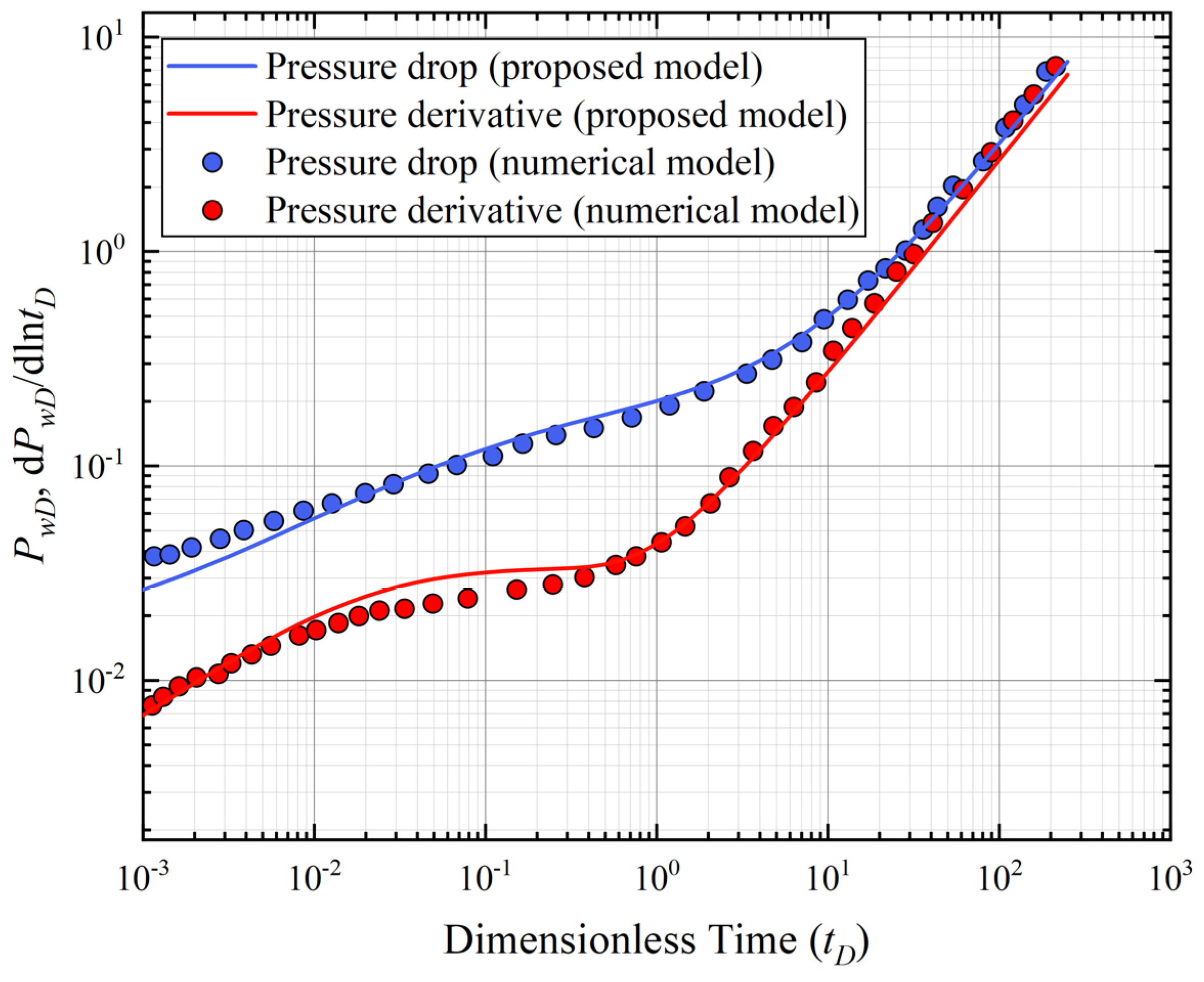
3. Model Validation

To validate the accuracy of the proposed model, a comparative analysis was conducted against a numerical model. The test case involved a reservoir comprising four heterogeneous blocks, with a fractured horizontal well producing at a constant rate of 30 m³/d. Additional model parameters are detailed in

Table 1. Other model parameters for the validation.

Parameters		Parameters
Reservoir lateral length (m)	1075	Fracture permeability (mD)	3000
Initial pressure (MPa)	20.29	Block 1 permeability (mD)	10
Wellbore radius (m)	0.1	Block 2 permeability (mD)	30
Matrix total compressibility (MPa−1)	0.02	Block 3 permeability (mD)	60
Formation spacing (m)	268	Block 4 permeability (mD)	90
Fracture half-length (m)	50	Oil viscosity (mPa·s)	4
Matrix porosity	0.125

. Figure 4 presents a comparison of the computational results obtained from the numerical model and the semi-analytical model. The results exhibit a favorable agreement in pressure transient behaviors, effectively validating the accuracy of the proposed model.

4. Results and Discussion

With the aid of the proposed model, the pressure transient behavior of the multi-fractured horizontal well in irregular heterogeneous reservoirs can be calculated. Subsequently, the flow regimes can be identified and analyzed, providing insights into the dynamic interactions between the well and the reservoir. The sensitivity analysis further explores the impact of crucial parameters, such as reservoir heterogeneity, drainage area heterogeneity, fracture length, and fracture conductivity, on the pressure response. The basic dimensionless parameters for different blocks are listed in

Table 2. Basic data for different blocks.

Parameters	Block 1	Block2	Block 3	Block 4	Block 5
Block width	4	4	4	4	4
Block length	4	7	8	6	5
Block permeability	0.2	0.4	0.6	0.4	0.2
Fracture conductivity	10	10	10	10	10
Fracture length	2	2	2	2	2
Formation thickness	0.2	0.2	0.2	0.2	0.2
Fracture width	1 × 10−4	1 × 10−4	1 × 10−4	1 × 10−4	1 × 10−4

. The parameter values used in this study were selected based on commonly reported ranges in the literature for unconventional reservoirs, ensuring their relevance to real-field conditions.

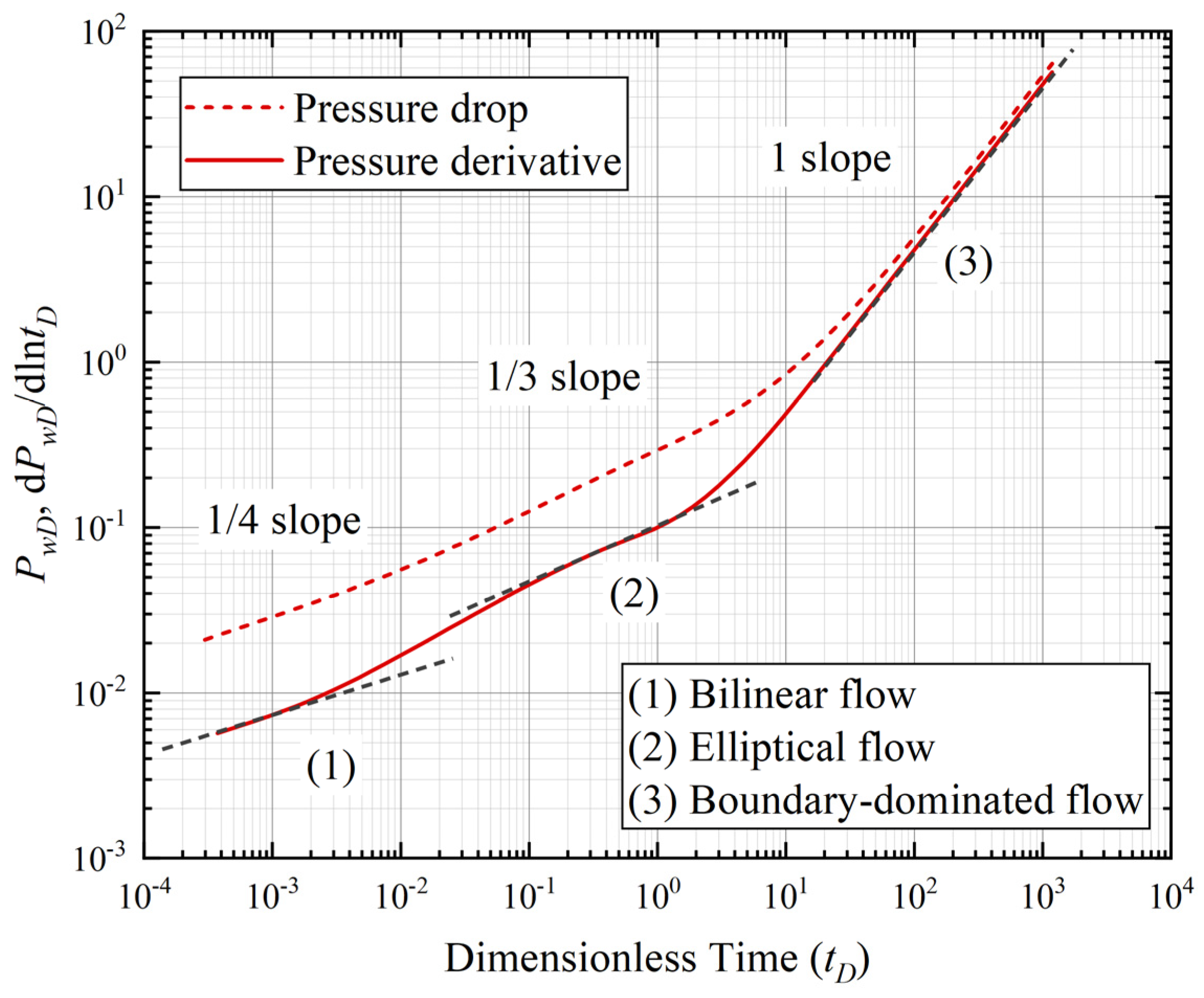
4.1. Flow Regimes Analysis

Though this model, the double logarithm diagram of pressure drop and pressure derivative are plotted in Figure 5. From this figure, one can find that three distinct flow regimes have been identified: bilinear flow, elliptical flow, and boundary-dominated flow [24]. The bilinear flow regime is observed during the early stages of production, where the pressure transient is primarily influenced by the simultaneous linear flow in both the matrix and the fracture network. This regime is characterized by a slope of 1/4 on the pressure derivative curve, indicating the dual linear flow paths. As the pressure transient propagates further into the reservoir, the flow regime transitions to elliptical flow. The pressure derivative curve during this regime exhibits a slope of 1/3, reflecting the radial-like flow in an elliptical geometry. In the late-time stage, the pressure transient reaches the reservoir boundaries, leading to the boundary-dominated flow regime. During this phase, the pressure derivative curve exhibits a unit slope, indicating that the reservoir is no longer infinite-acting and that the boundaries significantly influence the pressure behavior.

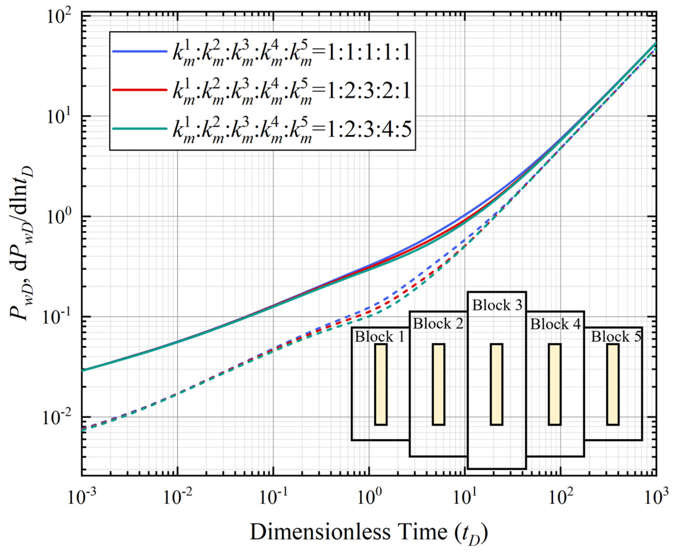
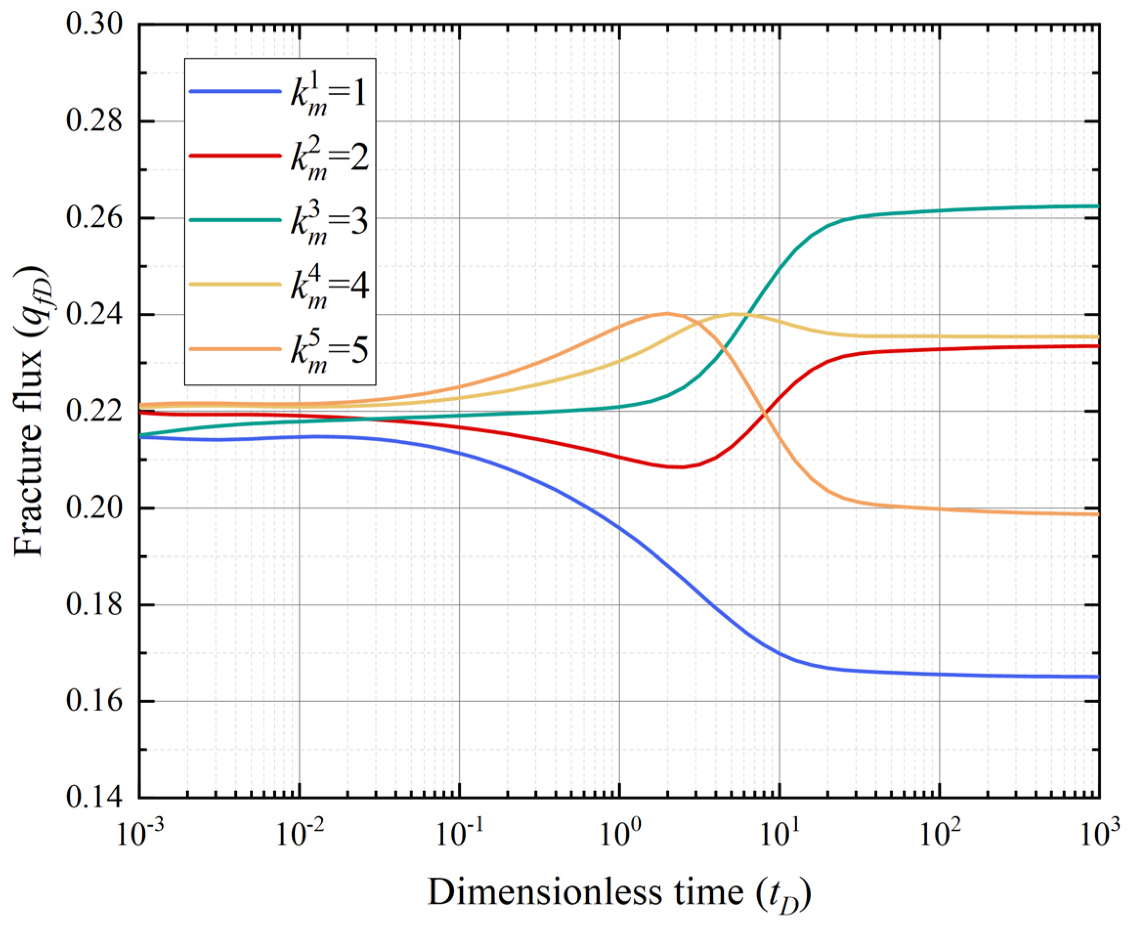
4.2. Different Permeability Ratios

In this section, the impact of permeability heterogeneity on transient pressure behavior in heterogeneous reservoirs with the irregular boundary are investigated. To systematically analyze the effects of different permeability distributions, we consider three distinct permeability combinations: (1, 1, 1, 1, 1), (1, 2, 3, 2, 1), and (1, 2, 3, 4, 5). The selected permeability distributions ensure a controlled sensitivity analysis, avoiding extreme contrasts that may not be realistic in practical reservoirs. As shown in Figure 6, one can find that the permeability heterogeneity presents a significant effect on the elliptical flow. As the permeability heterogeneity increases, the pressure front takes longer to propagate evenly through the lower-permeability zones, extending the duration of elliptical flow. Figure 7 shows the variation of fracture flux as a function of dimensionless time under different permeability ratios. It can be seen from this figure that the permeability heterogeneity mainly affects the flux distribution in the middle and late periods. As the permeability and drainage area increase, the flux through the fractures also increases. This trend is primarily attributed to the enhanced flow capacity of the reservoir, where higher permeability facilitates greater fluid movement, and a larger drainage area provides more contact for fluid extraction. However, for cases with permeability ratios of four and five, the fracture flux does not continue to increase despite the higher permeability. This deviation from the trend is due to the reduction in the drainage area, which limits the volume of fluid available for extraction. Thus, even though the reservoir’s flow capacity is improved by the higher permeability, the smaller drainage area becomes the limiting factor, preventing further increases in fracture flux.

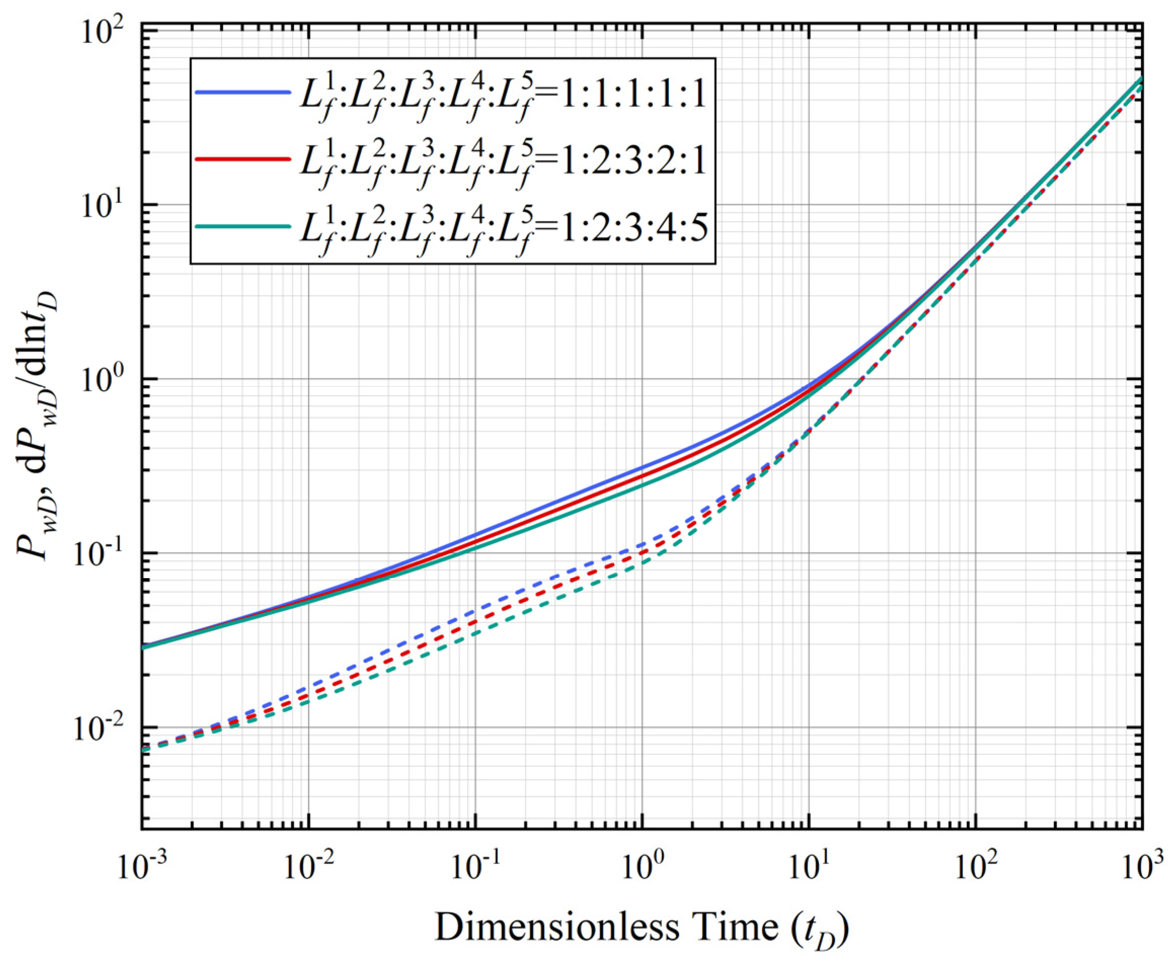
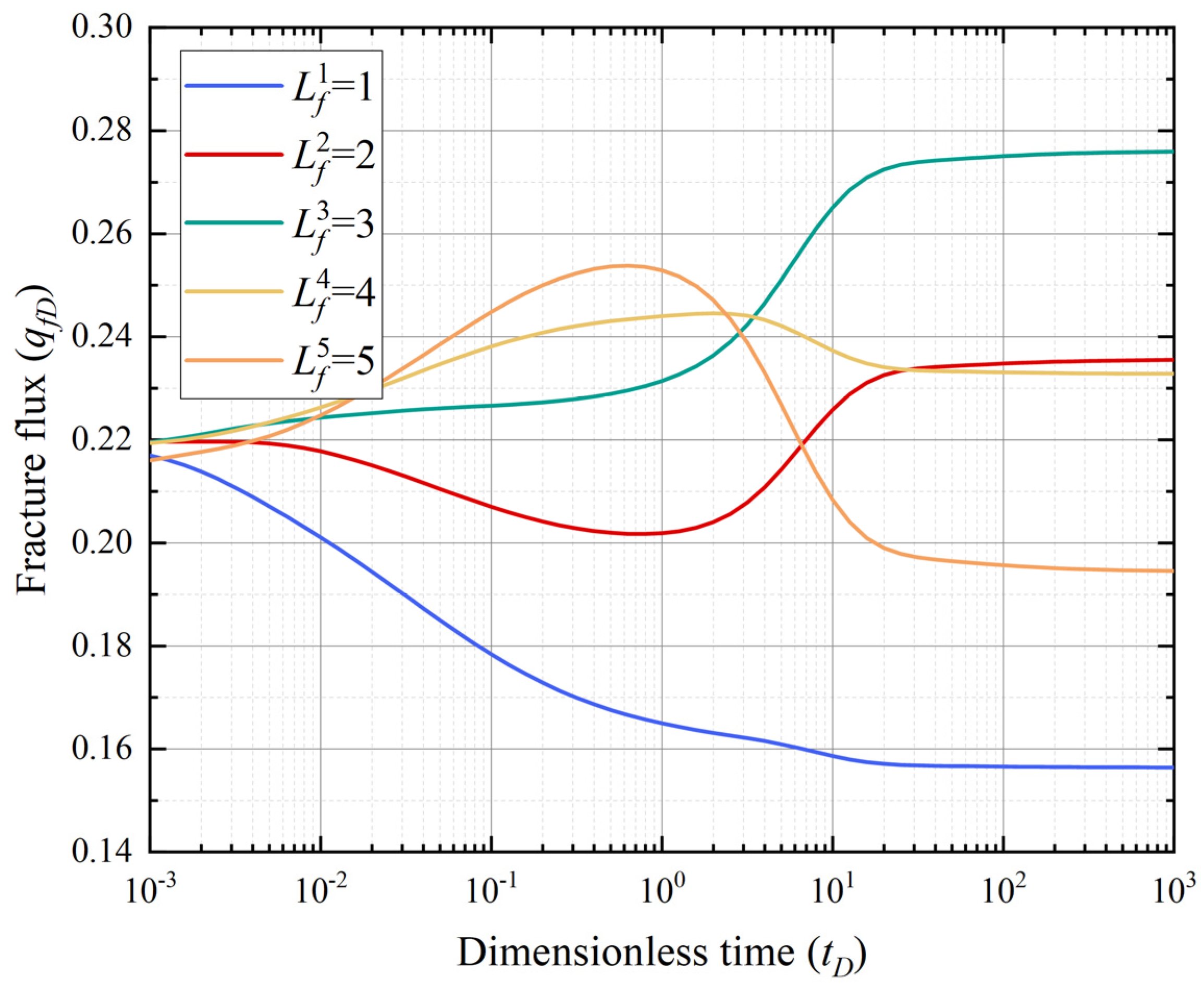
4.3. Fracture Length

Figure 8 shows the pressure drop and pressure derivative curves under different fracture lengths. In Figure 8, one can observe that the fracture length mainly affects the bilinear flow regime. As the fracture length increases, the duration of the bilinear flow increases [25]. This is because when the fracture length is larger, the distance that fluid must travel within the fractures increases significantly. Thus, the time required for the pressure transients to propagate through the entire fracture system also increases. Figure 9 shows the variation of fracture flux as a function of dimensionless time under different fracture lengths. As the fracture length increases, the flux through the fractures also increases. This trend occurs because longer fractures provide a greater contact area with the reservoir, enhancing fluid flow into the fracture network. However, due to the irregular reservoir geometry, different fractures are located in regions with varying drainage areas. For smaller drainage areas, even if the fracture length is increased, production will eventually decline as the recoverable reserves within the limited area are depleted.

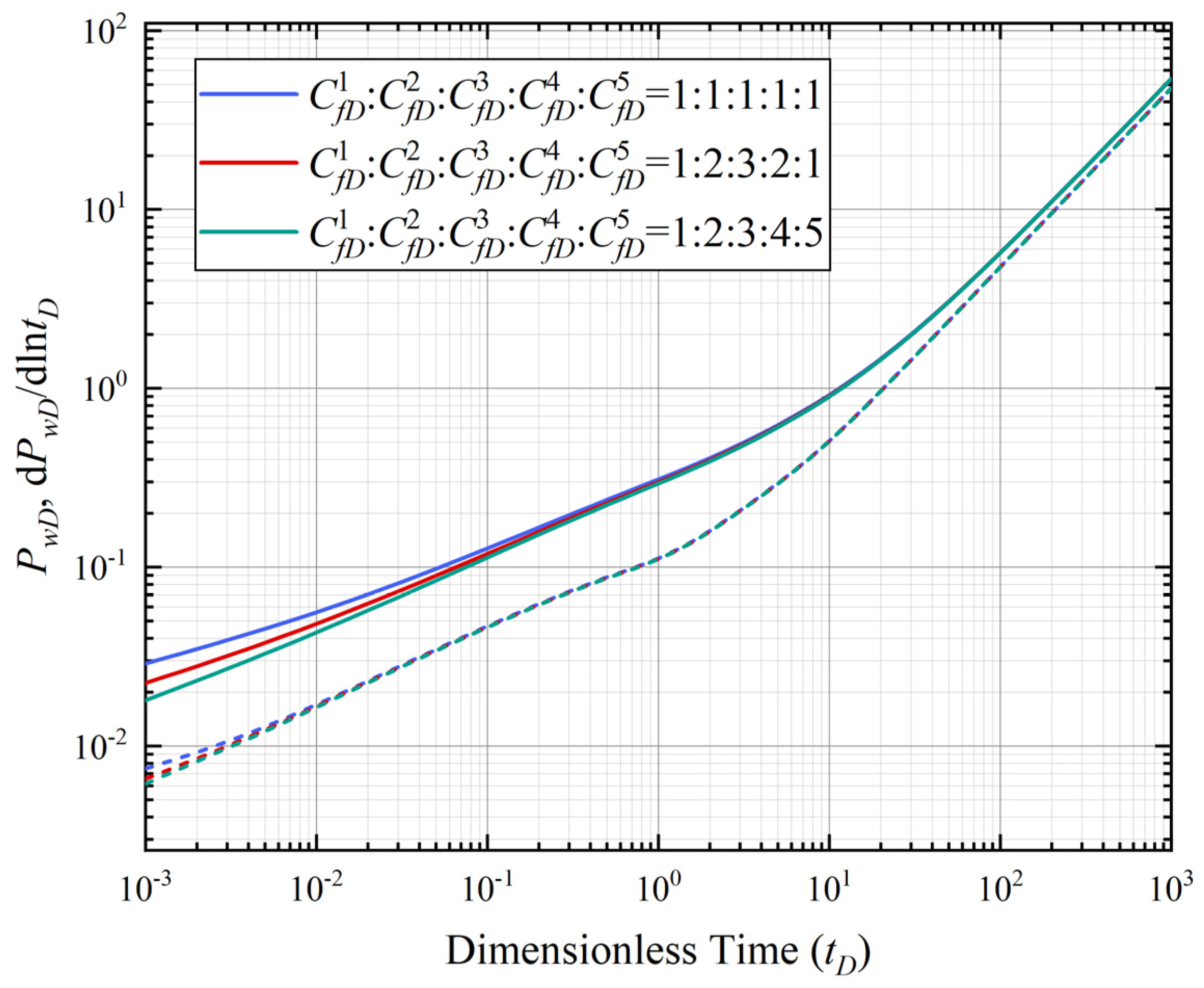
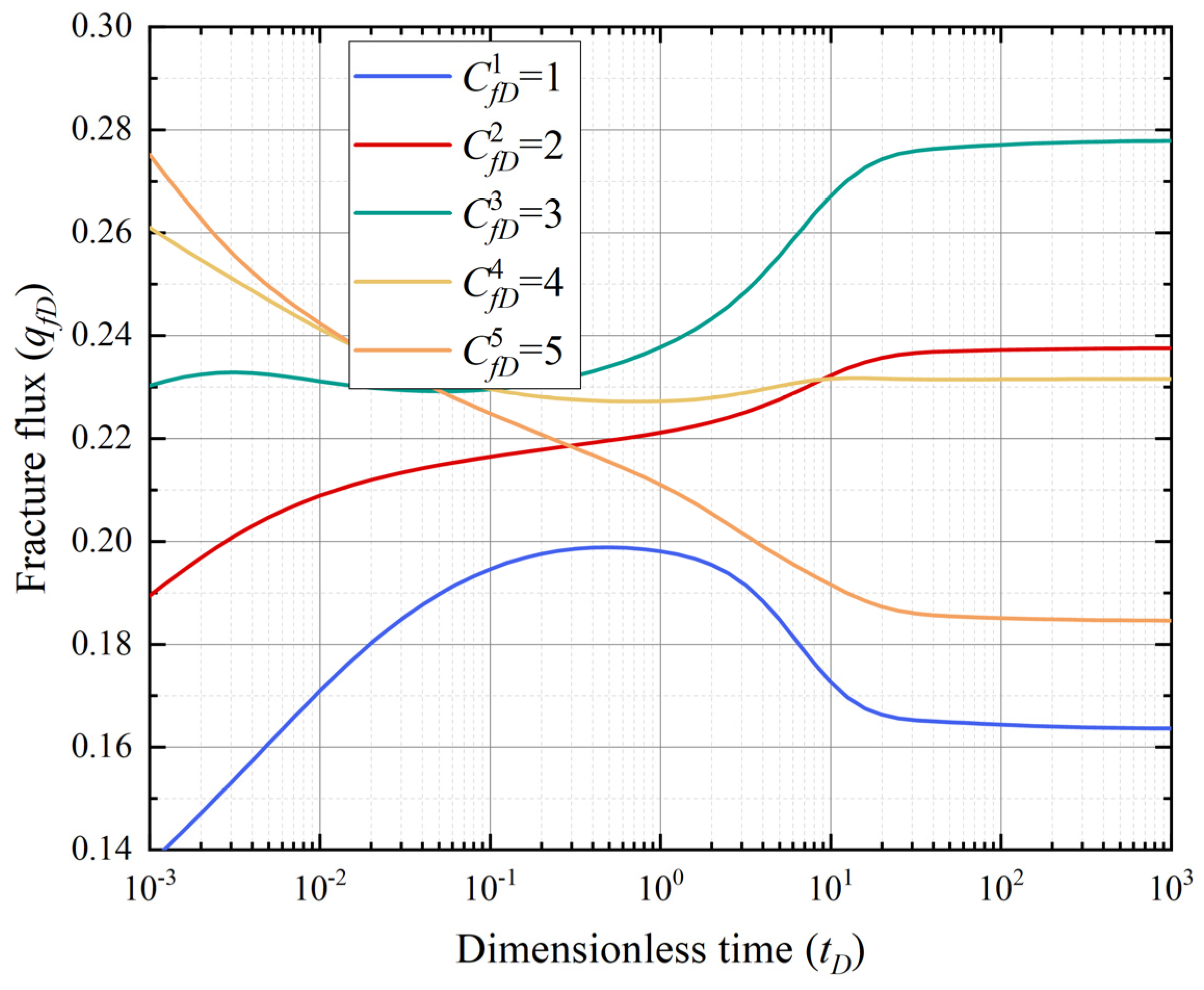
4.4. Fracture Conductivity

Figure 10 shows the pressure drop and pressure derivative curves under different fracture conductivity. As one can see from this figure, the fracture conductivity presents a significant impact on the early production period of the transient pressure behavior [26]. A higher fracture conductivity leads to a smaller pressure drop. This is because when fracture conductivity is high, fluids can flow more easily through the fractures with minimal resistance. This reduces the pressure loss as the fluid moves from the reservoir matrix to the wellbore. Figure 11 shows the variation of fracture flux as a function of dimensionless time under different fracture conductivity. Fracture conductivity has a significant impact on fracture flux throughout the entire production period. In the early stages, fracture flux is positively correlated with fracture conductivity because there is no influence from the drainage area limitation. During this phase, higher fracture conductivity allows for more efficient fluid flow from the reservoir into the fractures, resulting in increased flux. However, in the later stages of production, the drainage area becomes a limiting factor. As the accessible fluid volume diminishes, even with increased fracture conductivity, the fracture flux begins to decline. This occurs because the reduced drainage area restricts the amount of fluid available to enter the fractures, outweighing the benefits of enhanced conductivity. Thus, while fracture conductivity plays a critical role in maximizing flux initially, its impact is constrained by drainage area limitations in the later production stages.

5. Conclusions

A novel semi-analytical model was proposed to investigate the transient pressure behavior of a multi-fracture horizontal well in irregular heterogeneous reservoirs. With the aid of the proposed model, three flow regimes were identified during the production. The important conclusions in this work are listed below:

(1)

The proposed model successfully captures the transitions between bilinear, elliptical, and boundary-dominated flow, offering a robust framework for interpreting pressure transient data.

(2)

Permeability heterogeneity significantly impacts pressure transient behavior and fracture flux. A higher heterogeneity prolongs elliptical flow, but a smaller drainage area limits flux at high permeability ratios, preventing further increases.

(3)

Fracture length primarily affects bilinear flow duration and fracture flux. A longer fracture leads to a prolonged duration of bilinear flow and increases fracture flux due to the greater contact area.

(4)

Higher fracture conductivity reduces pressure drop and enhances early-stage fracture flux by enabling easier fluid flow. However, in later stages, drainage area limitations restrict fluid availability, causing flux to decline despite increased conductivity.

The proposed model is not directly applicable to reservoirs with highly complex boundary conditions. Future work will extend the model to gas reservoirs by incorporating pseudo-pressure and pseudo-time functions, enabling a more accurate analysis of gas flow dynamics in heterogeneous formations.

References

- Wang, H.; Ma, F.; Tong, X.; Liu, Z.; Zhang, X.; Wu, Z.; Li, D.; Wang, B.; Xie, Y.; Yang, L. Assessment of global unconventional oil and gas resources. Pet. Explor. Dev. 2016, 43, 925–940. [Google Scholar]
- Noorollahi, Y.; Naseer, M.N.; Siddiqi, M.M. (Eds.) Utilization of Thermal Potential of Abandoned Wells: Fundamentals, Applications and Research; Academic Press: Cambridge, MA, USA, 2022. [Google Scholar]
- Hosseinzadeh, M.; Tavakoli, V. Analyzing the impact of geological features on reservoir heterogeneity using heterogeneity logs: A case study of Permian reservoirs in the Persian Gulf. Geoenergy Sci. Eng. 2024, 237, 212810. [Google Scholar]
- Shen, X.; Liu, H.; Mu, L.; Lyu, X.; Zhang, Y.; Zhang, W. A semi-analytical model for multi-well leakage in a depleted gas reservoir with irregular boundaries. Gas Sci. Eng. 2023, 114, 204979. [Google Scholar]
- Liang, Y.Z.; Teng, B.L.; Luo, W.J. Study of the pressure transient behavior of directional wells considering the effect of non-uniform flux distribution. Pet. Sci. 2024, 21, 1765–1779. [Google Scholar]
- Peaceman, D.W. Fundamentals of Numerical Reservoir Simulation; Elsevier: Amsterdam, The Netherlands, 1977. [Google Scholar]
- Chen, Z.; Huan, G.; Ma, Y. Computational Methods for Multiphase Flows in Porous Media; Society for Industrial and Applied Mathematics: Philadelphia, PA, USA, 2006. [Google Scholar]
- Correia, M.G.; Maschio, C.; Schiozer, D.J. Integration of multiscale carbonate reservoir heterogeneities in reservoir simulation. J. Pet. Sci. Eng. 2015, 131, 34–50. [Google Scholar]
- Li, H.; Yu, H.; Cao, N.; Cheng, S.; Tian, H.; Di, S. Three-Dimensional Numerical Simulation of Multiscale Fractures and Multiphase Flow in Heterogeneous Unconventional Reservoirs with Coupled Fractal Characteristics. Geofluids 2021, 2021, 8265962. [Google Scholar]
- Khadivi, K. A numerical approach for permeability estimation in radially heterogeneous reservoirs. J. Porous Media 2022, 25, 1–15. [Google Scholar]
- Luo, J.; Hou, Z.; Feng, G.; Liao, J.; Haris, M.; Xiong, Y. Effect of reservoir heterogeneity on CO2 flooding in tight oil reservoirs. Energies 2022, 15, 3015. [Google Scholar] [CrossRef]
- Zhang, C.; Wang, X.; Jiang, C.; Zhang, H. Numerical simulation of geothermal energy production from hot dry rocks under the interplay between the heterogeneous fracture and stimulated reservoir volume. J. Clean. Prod. 2023, 414, 137724. [Google Scholar]
- Brown, M.; Ozkan, E.; Raghavan, R.; Kazemi, H. Practical solutions for pressure-transient responses of fractured horizontal wells in unconventional shale reservoirs. SPE Reserv. Eval. Eng. 2011, 14, 663–676. [Google Scholar]
- Stalgorova, E.; Mattar, L. Practical analytical model to simulate production of horizontal wells with branch fractures. In Proceedings of the SPE Canada Unconventional Resources Conference, Calgary, AB, Canada, 30 October–1 November 2012; SPE: Garden Grove, CA, USA, 2012. Paper Number: SPE-162515. [Google Scholar]
- Shi, J.; Vishal, V.; Leung, J.Y. Uncertainty assessment of vapex performance in heterogeneous reservoirs using a semi-analytical proxy model. J. Pet. Sci. Eng. 2014, 122, 290–303. [Google Scholar]
- Cheng, L.; Fang, S.; Wu, Y.; Lu, X.; Liu, H. A hybrid semi-analytical model for production from heterogeneous tight oil reservoirs with fractured horizontal well. J. Pet. Sci. Eng. 2017, 157, 588–603. [Google Scholar]
- Tian, F.; Wang, X.; Xu, W. A semi-analytical model for multiple-fractured horizontal wells in heterogeneous gas reservoirs. J. Pet. Sci. Eng. 2019, 183, 106369. [Google Scholar]
- Li, Z.; Wu, X.; Han, G.; Zhang, L.; Zhao, R.; Shi, S. A semi-analytical pressure model of horizontal well with complex networks in heterogeneous reservoirs. J. Pet. Sci. Eng. 2021, 202, 108511. [Google Scholar]
- Ren, J.; Wu, Q.; Liu, X.; Zhang, H. Semi-analytical modeling for multi-wing fractured vertical wells in a bilaterally heterogeneous gas reservoir. J. Nat. Gas Sci. Eng. 2021, 95, 104203. [Google Scholar]
- Deng, Q.; Qu, J.; Mi, Z.; Xu, B.; Lv, X.; Huang, K.; Zhang, B.; Nie, R.-S.; Chen, S. Performance of multistage-fractured horizontal wells with secondary discrete fractures in heterogeneous tight reservoirs. J. Pet. Explor. Prod. Technol. 2024, 14, 975–995. [Google Scholar]
- Medeiros, F.; Ozkan, E.; Kazemi, H. A semianalytical approach to model pressure transients in heterogeneous reservoirs. SPE Reserv. Eval. Eng. 2010, 13, 341–358. [Google Scholar]
- Peaceman, D.W. Interpretation of well-block pressures in numerical reservoir simulation with nonsquare grid blocks and anisotropic permeability. Soc. Pet. Eng. J. 1983, 23, 531–543. [Google Scholar]
- Stehfest, H. Remark on algorithm 368: Numerical inversion of Laplace transforms. Commun. ACM 1970, 13, 624. [Google Scholar]
- Teng, B.; Andy Li, H. Pressure-transient behavior of partially penetrating inclined fractures with a finite conductivity. SPE J. 2019, 24, 811–833. [Google Scholar]
- Wang, J.; Wang, X.; Dong, W. Rate decline curves analysis of multiple-fractured horizontal wells in heterogeneous reservoirs. J. Hydrol. 2017, 553, 527–539. [Google Scholar]
- Chen, X.; Liu, P. Pressure transient analysis of a horizontal well intercepted by multiple hydraulic fractures in heterogeneous reservoir with multiple connected regions using boundary element method. J. Hydrol. 2023, 616, 128826. [Google Scholar]