Sample-Based Optimal Dispatch of Shared Energy Storage in Community Microgrids Considering Uncertainty

Abstract

Shared energy storage (SES) in communities equipped with renewable energy sources (RESs) can effectively maintain power supply reliability. However, the dispatch of SES is highly influenced by the uncertainty of RES output. Traditional optimization approaches, such as chance-constrained optimization (CC) and robust optimization (RO), have limitations. The former relies heavily on distribution information, while the latter tends to be overly conservative. The above problems are prominent when the size of available samples is limited. To address this, we introduce the concept of statistical feasibility and propose a sample-based robust optimization approach. This approach constructs the uncertainty set through shape learning and size calibration based solely on the sample set and further reconstructs it by introducing constraint information. Our numerical studies show that the proposed approach can obtain feasible optimal results with a 10.82% cost increase compared to deterministic optimization, and the reconstruction of the uncertainty set can increase the level of utilization of the stability requirement to around 0.05. Comparisons with several traditional optimization approaches demonstrate the effectiveness of the proposed approach.

1. Introduction

Energy storage can provide significant flexibility for new power systems with high penetration of renewable energy sources (RESs), so it has been well studied in the past [1]. In community microgrids, the adoption of shared energy storage (SES) can enhance the utilization of clean and low-cost energy, thereby reducing electricity costs. However, the uncertainty of RES output may introduce challenges in the dispatch of SES, which needs to be taken seriously and effectively addressed [2].

The main uncertainty in community microgrids arises from the inaccuracy of the forecasted RES output, such as wind and solar power [3,4]. If the output curves of wind and solar power could be accurately obtained, i.e., their distribution information was known, then stochastic optimization (SO) [5] or chance-constrained optimization (CC)  [6] could be applied. However, accurate knowledge in this regard is generally not available, and research is often based only on limited samples. In this case, traditional approaches for dealing with uncertainty may become infeasible [7].

To address this issue, we propose a data-driven approach that relies solely on samples to optimize the dispatch of SES in community microgrids. We first introduce the concept of statistical feasibility to measure the quality of the available samples and transform the traditional CC problem into a sample-based robust optimization (SRO) problem. Furthermore, by introducing constraint information and reconstructing the uncertainty set, the SRO is converted into a reconstructed sample-based robust optimization (RSRO), the conservativeness of which is significantly reduced. Finally, solution methodologies are provided for the uncertain parameters in both the objective function and the constraints, ensuring that the proposed approach can solve the problem efficiently.

1.1. Related Works

In the numerous studies conducted on SES, the method of handling uncertainty has garnered significant attention. Bayram et al. studied the architecture of SES in residential scenarios, where the uncertainty of different users’ power demands was taken into account [8]. To maximize the arbitrage of SES, Dai et al. used robust optimization (RO) to carry out an interaction game among multiple users under energy price uncertainty [9]. In addition, uncertainty also exists on the energy supply side, which directly affects the stable operation of the SES system, making it crucial to address this issue properly [10,11]. Wang et al. used a Bayesian robust optimization model to solve the energy storage optimization problem, where the output uncertainty of wind and solar power was addressed by generating scenarios to fit the forecasted output curves [12]. Similarly, the uncertainties on both the supply and demand sides were given significant attention in day-ahead optimization in order to obtain the optimal demand response strategy with SES [13].

The volatility of wind and photovoltaic (PV) power output in microgrids is the main source of uncertainty in microgrid systems. Generally, existing research deals with this uncertainty problem from two perspectives. One is to make a probabilistic prediction of wind and PV output, and then optimize energy dispatch based on the predicted value. For example, Mehrjerdi et al. used Gaussian distribution to assume the output characteristics of PV in building systems to deal with uncertainty, and then optimized the coordination of hydrogen storage and fuel cells [14]. Lu et al. used randomly generated scenarios to describe the uncertainty of RES output and completed the modeling of multi-microgrid system dispatch [15]. In addition, random process simulation methods such as Monte Carlo simulation and Markov chain have also been used [16]. The other perspective is to give interval constraints and use the worst-case scenario for optimal dispatch to ensure the robustness of results. For example, in  [17], the uncertainty of the electricity generated by solar panels was measured by the upper and lower limit output constraints to complete the construction of an optimal dispatch model for energy storage. Both kinds of methods require obtaining prior information about the distribution of uncertain parameters. In reality, RES output prediction is generally based on historical data. How to perform optimal dispatch based only on known historical samples is a problem worth studying.

The performance of different approaches varies depending on the information of uncertain parameters we can obtain when solving the problem. If the distribution information of uncertain parameters is known, approaches such as scenario generation(SG) or CC can handle the issue. Walker et al. represented the distribution of uncertain parameters using a discrete finite sample set to design the control strategy for SES in residential scenarios [18]. Chance-constrained optimization was used by Huang et al. to address the uncertainties present in household energy management [19]. However, the aforementioned approaches have high requirements for the specific distribution information of uncertain parameters and pose significant computational challenges in multi-scenarios and probabilistic constraint settings. RO is often used to handle optimization problems with unknown distributions of uncertain parameters [20,21]. However, since it requires ensuring that constraints are met under worst-case scenarios with small probabilities, the results tend to be very conservative [22]. As a result, some researchers have adopted distributionally robust optimization (DRO) methods, which reduce the need for unavailable information while making the optimization results less conservative [23,24]. However, DRO still requires assumptions about the distribution of uncertain parameters rather than being entirely data-driven and based on the current samples when solving optimization problems [25].

In summary, there are two gaps in the current research. The first one concerns how to use only historical samples instead of prior information of uncertain parameters for SES dispatch, and the other concerns how to reduce the dependence of traditional approaches on uncertain parameter distribution characteristics. To address the shortcomings above, we propose our approach based on the concept of statistical feasibility [26], which is entirely based on sample data and avoids reliance on the specific distribution of uncertain parameters [27]. Additionally, by constructing and reconstructing the robust uncertainty set, our approach can continuously reduce the conservativeness of the optimization results. Specifically, a comparison between our approach and existing methods is shown in

Table 1. Literature review.

Ref No.	Approach	Uncertainty Sources	Characterization Method	Distribution Independency	Statistical Feasibility
[10]	CC	wind output	normal distribution	×	×
[11,15]	SG	PV output	scenario generation	×	×
[14]	SG	PV output	Gaussian distribution	×	×
[18]	SG	PV output	Monte Carlo simulation	×	×
[12,13,20]	RO	wind and PV output	interval uncertainty	✓	×
[17]	RO	PV output	interval uncertainty	✓	×
[24]	RO	wind output	interval uncertainty	✓	×
[16]	RO	wind and PV output	Markov chain	✓	×
[24]	DRO	PV output	interval uncertainty	✓	×
our approach	SRO, RSRO	wind output	sample dataset	✓	✓

below.

1.2. Our Contributions

The contributions of this paper are as follows:

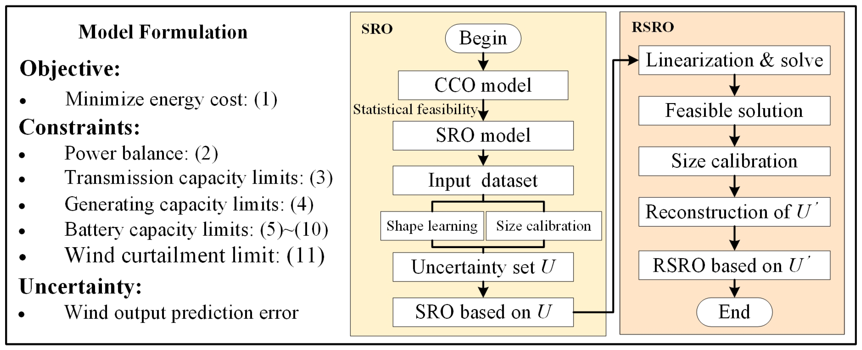
• We have constructed a community microgrid model with SES under deterministic and chance-constrained conditions with wind output uncertainty. The model is transformed into SRO and RSRO by introducing the concept of statistical feasibility. The uncertainty set is constructed and reconstructed based only on samples and constraint information, gradually reducing the conservatism of the proposed approach.
• The uncertainty in the objective function is handled using the sample average approximation (SAA) method, and the nonlinear terms in the constraints are dealt with using Slater’s condition, thereby enabling the practical solution of the proposed RSRO approach.
• The proposed approach is tested using a community example with three microgrids. Benchmarks and evaluation metrics are developed to verify the effectiveness of the approach. Compared with traditional approaches, the optimization results demonstrate the proposed approach’s superiority.

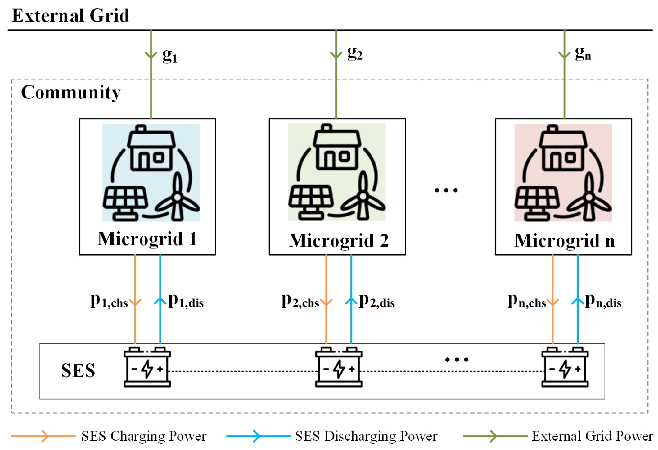
Section 2 constructs the community microgrid model with SES, including deterministic and opportunity-constrained conditions. Section 3 introduces the concept of statistical feasibility and transforms the problem into SRO and RSRO, highlighting the construction of the uncertainty set. Section 4 and Section 5 present the solution methodology and numerical studies, respectively. Finally, Section 6 concludes the paper.

2. System Model

This section establishes a community model comprising multiple microgrids equipped with SES to meet the energy utilization and storage needs of the entire community. Each microgrid contains renewable energy generation stations and user loads while also being connected to the external grid to ensure power stability. Figure 1 illustrates the detailed system structure.

To simplify the problem, several reasonable assumptions are made for the system, specifically including the following:

• The generation cost of renewable energy is assumed to be zero.
• The SES system can only charge or discharge at any given moment concerning each microgrid. However, its charging and discharging states can vary between different microgrids.
• The charging and discharging efficiency of the SES system is considered to be constant.

2.1. Deterministic Model

The community operator aims to meet the user’s power demand at the lowest cost. The objective function is detailed as follows:

$$\mathbf{\left(}\mathbf{PO}\mathbf{\right)} min\sum _t^T\sum _i^N\Delta t\left({\lambda }_{grid}^t{g}_i^t+\gamma {\omega }_{i,cur}^t+C_{SES}\left(p_{i,dis}^t+p_{i,chs}^t\right)\right)$$

(1)

where t and T denote the index and set of time periods, and i and N denote the index and set of microgrids. $\Delta t$ is a time interval. ${\lambda }_{grid}^t$ refers to the power price of the external grid. $g_i^t$ and ${\omega }_{i,cur}^t$ denote the output of the external grid and renewable energy curtailment in microgrid i at time t, respectively. The curtailment penalty is $\gamma$, and the variable cost of SES is denoted as $C_{SES}$. The SES’s charging and discharging power in microgrid i at time t are denoted by $p_{i,chs}^t$ and $p_{i,dis}^t$, respectively.

The decision variables in the above equation are $g_i^t$, $p_{i,dis}^t$, and $p_{i,chs}^t$. The three terms in the objective function represent, in order, the cost of purchasing electricity from the external grid, the cost of curtailing wind and solar power, and the cost of energy storage, charging, and discharging losses.

For any microgrid within the community, it is necessary to maintain a power balance in the system at any given time, that is,

$$g_i^t+{\omega }_i^t-{\omega }_{i,cur}^t+p_{i,dis}^t-p_{i,chs}^t=d_i^t$$

(2)

where ${\omega }_i^t$ and $d_i^t$ denote the output of renewable energy and load in microgrid i at time t.

The left side of the equation represents the total power generation of microgrid i at time t, which includes the input power from the external grid, the renewable energy generation, and the net discharge of energy storage. The right side of the equation represents the corresponding total load.

The power transmitted from the external grid to the microgrid must satisfy the transmission line power limit, yielding the transmission line capacity constraint.

$$0\le g_i^t\le \overline{g_i^t}$$

(3)

where $\overline{g_i^t}$ denotes the output limit of the external grid for microgrid i at time t.

The constraint related to renewable energy within the microgrid is the maximum generation capacity constraint:

$$0\le {\omega }_i^t\le \overline{{\omega }_i^t}$$

(4)

where $\overline{{\omega }_i^t}$ represents the maximum forecasted output of renewable energy.

For the SES within the community, the constraints that need to be satisfied are as follows:

$$0\le E^t=E^{t-1}+\sum _i^N\left(\eta p_{i,chs}^t-{\displaystyle \frac{p_{i,dis}^t}{\eta }}\right)\le \overline{E}, \forall t\ge 1$$

(5)

$$E^t={\displaystyle \frac{\overline{E}}{2}},t=0$$

(6)

$$0\le p_{i,dis}^t\le \overline{p_{i,dis}}{u}_{i,dis}^t$$

(7)

$$0\le p_{i,chs}^t\le \overline{p_{i,chs}}{u}_{i,chs}^t$$

(8)

$$u_{i,dis}^t+u_{i,chs}^t=1$$

(9)

$$u_{i,dis}^t,u_{i,chs}^t\in \{0,1\}$$

(10)

where $E^t$ denotes the capacity of SES at time t, and its maximum is denoted as $\overline{E}$. The efficiency of the SES is set to $\eta$. $\overline{p_{i,dis}}$, and $\overline{p_{i,chs}}$ denotes the limit of discharge and charge in microgrid i. In addition, $u_{i,dis}^t$ and $u_{i,chs}^t$ indicate whether the SES has a discharging or charging status, with a value of 1 indicating Yes and a value of 0 meaning No.

Equations (5) and (6) describe the capacity limits of SES, requiring its capacity to remain within the allowable range at any given time, with the initial capacity set at half of the maximum capacity. Equations (7) and (8) impose limits on the maximum discharge and charge power, respectively. Equation (9) denotes that the SES can only be in a charging or discharging state concerning any individual microgrid. Finally, Equation (10) describes the values of the charge and discharge state variables.

Finally, in order to promote the consumption of renewable energy within the microgrid, an upper limit on curtailed wind and solar power is set, which is expressed as follows:

$$0\le {\omega }_{i,cur}^t\le \overline{{\omega }_{i,cur}^t}$$

(11)

where $\overline{{\omega }_{i,cur}^t}$ denotes the curtailment limit of renewable energy in microgrid i at time t.

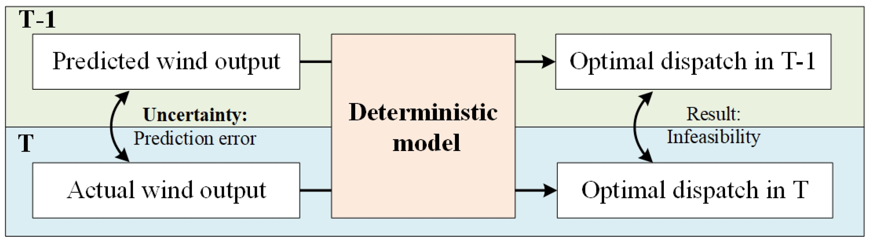
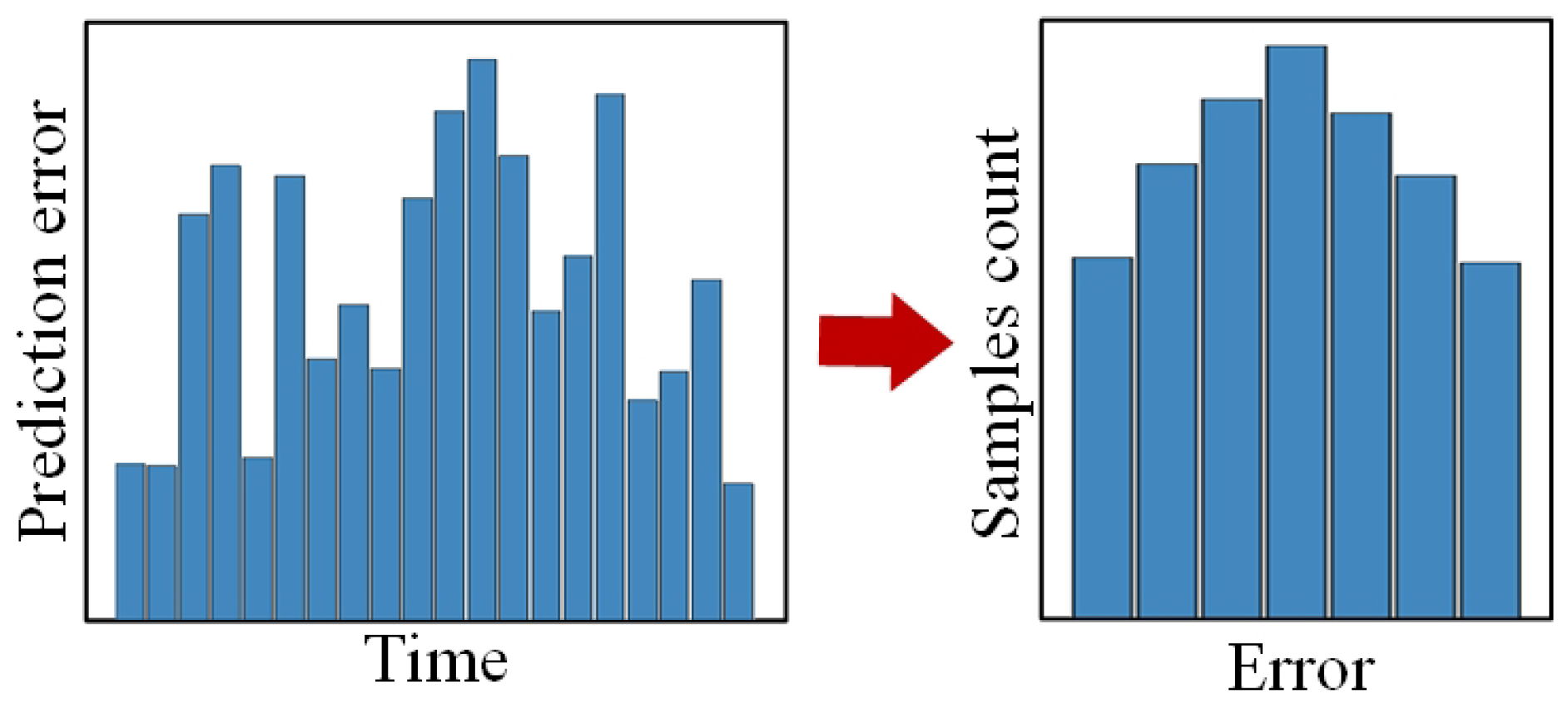
2.2. Uncertainty Analysis

In the previous section, we introduce the model for a community microgrid with SES under deterministic conditions, where neither the objective function nor the constraints include uncertain parameters. The deterministic model is obtained based on the known wind power output, and the predicted value is generally used as a substitute for calculation. However, the wind power output is significantly affected by meteorological conditions and fluctuates significantly, resulting in a certain gap between the actual and predicted output values, which is the source of uncertainty in the system. The explanation of uncertainty in the system is shown in Figure 2, where T − 1 refers to the dispatch formulation stage, and T refers to the real-time stage.

In order to measure the magnitude of wind power output fluctuations, the prediction error decomposition method is used to characterize the uncertainty in wind output prediction. The time-varying prediction error is expressed equivalently by the error parameter value and its sample count, as detailed in Figure 3.

Specifically, we use $\widetilde{{\omega }_i^t}$ to denote the predicted output of renewable energy so that the practical output can be expressed as the sum of the predicted one and the prediction error, as shown below:

$${\omega }_i^t=\widetilde{{\omega }_i^t}+{\xi }_i^t$$

(12)

2.3. Chance-Constrained Model

Based on the uncertainty analysis, a CC model is employed to define the constraints as still being met at a given confidence level to assess the satisfaction of constraints in the system when uncertainty is introduced. In detail, Equation (11) is reconstructed into the following corresponding chance-constrained form, with the confidence level set to $\rho$.

$$\mathbb{P}\left({\omega }_{i,cur}^t\le \overline{{\omega }_{i,cur}^t}\right)\ge 1-\rho$$

(13)

Because ${\omega }_{i,cur}^t$ varies with the variables $g_i^t,p_{i,dis}^t,\mathrm{and}{p}_{i,chs}^t$, we can define it as the function $\mathrm{H}(·)$. Additionally, $\mathbf{a}$ is used to denote the variable set $\{g_i^t,p_{i,dis}^t,p_{i,chs}^t\}$, so it can be determined that ${\omega }_{i,cur}^t=\mathrm{H}\left(\mathbf{a},{\xi }_i^t\right)$. Therefore, the original PO problem can be transformed into a chance-constrained optimization (CC) problem, as detailed below:

$$\mathbf{\left(}\mathbf{CC}\mathbf{\right)}min\sum _t^T\sum _i^N\Delta t\left({\lambda }_{grid}^t{g}_i^t+\gamma \mathrm{H}\left(\mathbf{a}(i,t),{\xi }_i^t\right)+C_{SES}\left(p_{i,dis}^t+p_{i,chs}^t\right)\right)$$

(14)

$$s.t.Constraints\left(2\right)–\left(10\right),\left(13\right)$$

3. Sample-Based RO

In this section, we first introduce a sample-based approach for handling the CC problem. Then, based on the system model established in the previous section, the problem is transformed into a tractable RO problem for to obtain a solution.

3.1. Statistical Gurantee

To handle CC, it is necessary to know the probability distribution of the uncertain parameters, i.e., $\mathbb{P}\left(\xi \right)$. However, in many cases, this requirement cannot be satisfied. In this study, for example, renewable energy output is influenced by various factors, such as equipment conditions and weather, making it difficult to determine its exact probability distribution. Typically, energy dispatch is carried out using predicted output, but the prediction error is also hard to grasp, especially when the number of samples is insufficient. In order to address this issue, the concept of statistical feasibility is introduced.

Definition 1

(Statistical Feasibility [26]). Consider the standard CC: $minf\left(x\right),s.t.\mathbb{P}\left(g\right(x,\xi )\in \mathcal{A})\ge 1-\rho$, where x is the decision variable, $\xi$ is the uncertain parameter, and $\mathcal{A}$ is feasible region. $D_{\xi }=\{{\xi }_1,{\xi }_2,\cdots ,{\xi }_n\}$ denotes a continuous i.i.d. data set. We consider an approach to have statistical feasibility when the optimal solution it generates, denoted as $x^{*}$, can satisfy the constraints at a certain confidence level for any given $D_{\xi }$.

$${\mathbb{P}}_{D_{\xi }}\left({\mathbb{P}}_{\xi }\left(g\left(x^{*},\xi \right)\in \mathcal{A}\right)\ge 1-\rho \right)\ge 1-\delta$$

(15)

Equation (15) can be understood from two perspectives. First, the inner part is a probabilistic constraint, similar to traditional CC, requiring that the constraints be satisfied with a probability of $1-\rho$ as the value of the uncertain variable $\xi$ changes. The outer part is significantly different. Its uncertainty arises from selecting the sample set $D_{\xi }$, requiring that the inner constraint is satisfied at a confidence level of $1-\delta$ for all possible sample sets. This is the essential difference between statistical feasibility and traditional CC.

A simple RO, similar to the CC illustrated in Definition 1, can be formulated as $minf\left(x\right),s.t.g(x,\xi )\in \mathcal{A},\forall x\in \mathcal{U}$, where $\mathcal{U}$ is the uncertainty set in RO. RO requires that the constraint $g(x,\xi )\in \mathcal{A}$ be satisfied for any feasible point within the uncertainty set $\mathcal{U}$. If we appropriately select $\mathcal{U}$ such that it covers the range of all possible values of $\xi$ within $1-\rho$, i.e., making $\mathcal{U}$ satisfy $\mathbb{P}\left(\xi \in \mathcal{U}\right)\ge 1-\rho$, then the solution x generated by RO is guaranteed to satisfy CC [26], that is,

$$\mathbb{P}\left(g\left(x,\xi \right)\in \mathcal{A}\right)\ge \mathbb{P}\left(\xi \in \mathcal{U}\right)\ge 1-\rho$$

(16)

It is worth noting that the first inequality in Equation (16) arises from the inherent conservation of the RO approach. The above equation provides a method for transforming CC into RO when a specific sample set is given.

In the context where renewable energy output cannot be accurately predicted, and only a limited number of prediction error samples can be collected, the above theory is directly applied to the model proposed in this study. Based on the definition of statistical feasibility, Equation (13) can be transformed into

$${\mathbb{P}}_{D_{\xi }}\left({\mathbb{P}}_{\xi }\left(\mathrm{H}\left(\mathbf{a}(i,t),{\xi }_i^t\right)\le \overline{{\omega }_{i,cur}^t}\right)\ge 1-\rho \right)\ge 1-\delta$$

(17)

Furthermore, by establishing an uncertainty set $\mathcal{U}\left(\xi \right)$ that covers the $1-\rho$ portion of the possible values of $\xi$ with a confidence level of $1-\delta$, i.e., $\mathbb{P}\left(\mathbb{P}\left({\xi }_i^t\in \mathcal{U}\left(\xi \right)\right)\ge 1-\rho \right)\ge 1-\delta$, Equation (17) can be transformed into

$$\mathrm{H}\left(\mathbf{a},{\xi }_i^t\right)\le \overline{{\omega }_{i,cur}^t},\forall {\xi }_i^t\in \mathcal{U}$$

(18)

Based on the above analysis, the CCO problem can be transformed into a sample-based robust optimization (SRO) problem as follows:

$$\mathbf{\left(}\mathbf{SRO}\mathbf{\right)}min\sum _t^T\sum _i^N\Delta t\left({\lambda }_{grid}^t{g}_i^t+\gamma \mathrm{H}\left(\mathbf{a}(i,t),{\xi }_i^t\right)+C_{SES}\left(p_{i,dis}^t+p_{i,chs}^t\right)\right)$$

(19)

$$s.t.Constraints\left(2\right)–\left(10\right),\left(18\right)$$

3.2. Uncertainty Set Construction

The above discussion motivates us to seek appropriate methods for constructing the uncertainty set $\mathcal{U}$. Considering the conservativeness of RO and the convenience of solving the problem, the selection of $\mathcal{U}$ is expected to follow the following principles:

• It is necessary to find the smallest possible uncertainty set that satisfies the given conditions, which means that $\mathcal{U}$ should cover the high-probability regions (HPRs) [28] of $\xi$. This approach will better capture the distributional characteristics of $\xi$ and reduce conservatism.
• The shape of the uncertainty set affects the complexity of the problem. In this study, $\mathcal{U}$ with the shape of an ellipsoid is chosen to reduce the computational difficulty [29].

Given a sample set $D_{\xi }$ containing i.i.d. $\xi$ with a sample size of n, we divide it into two subsets, denoted as $D_{{\xi }_1}$ and $D_{{\xi }_2}$, with sample sizes of $n_1$ and $n_2$, respectively. The uncertainty set $\mathcal{U}$ is determined through the following two steps:

Step 1 (shape learning): Assume that the samples in $D_{{\xi }_1}$ are located within an ellipsoid, denoted as $D_{{\xi }_1}=\left\{\xi \right|{(\xi -\mu )}^{\top }{\Sigma }^{-1}(\xi -\mu )\le s_1\}$, where $\mu$ is the sample mean in $D_{{\xi }_1}$, $\Sigma$ is the sample covariance matrix, and $s_1$ is a scalar that reflects the size of the uncertainty set.

Step 2 (size calibration): The size of the uncertainty set is determined using $D_{{\xi }_2}$. First, we define a mapping $t(·)=\left\{{(\xi -\mu )}^{\top }{\Sigma }^{-1}(\xi -\mu )\right\}$ that reduces the dimension of the parameter $\xi$ to a scalar. Then, the shape formulated from Step 1 is equivalent to $\left\{\xi \right|t\left(\xi \right)\le s\}$. The value of s is determined using the quantile estimation method. By sorting $t\left(\xi \right)$ in ascending order to obtain $t\left({\xi }_{\left(k^{*}\right)}\right)$, where $t\left({\xi }_{\left(1\right)}\right)\le t\left({\xi }_{\left(2\right)}\right)\le \cdots \le t\left({\xi }_{\left(n_2\right)}\right)$, the indices corresponding to the $1-\rho$ content with the confidence level $1-\delta$ satisfy the following:

$$k^{*}=min\left\{i:\sum _{k=0}^{i-1}{C}_k^{n_2}{\left(1-\rho \right)}^k{\rho }^{n_2-k}\ge 1-\delta ,1\le i\le n_2\right\}$$

(20)

According to Equation (20), $s_1$ can be obtained by $s_1=t\left({\xi }_{\left(k^{*}\right)}\right)$. It is worth noting that Equation (20) must satisfy the existence condition [30]: $1-{(1-\rho )}^{n_2}\ge 1-\delta$, i.e.,  $n_2\ge {log}_{1-\rho }\left(\delta \right)$. In summary, based on the parameters $\mu$, $\Sigma$, and $s_1$, the uncertainty set $\mathcal{U}$ can be obtained, ensuring that Equation (18) is satisfied. The process of constructing the uncertainty set is summarized in Algorithm 1.

Algorithm 1 Uncertainty Set Construction of SRO

1: Initialize $D_{\xi }, n, \rho , \delta$ 2: Devide $D_{\xi }$ into subset $D_{{\xi }_1}$ and $D_{{\xi }_2}$, with sample sizes of $n_1$ and $n_2$, respectively 3: Calculate $\mu$ and $\Sigma$ based on subset $D_{{\xi }_1}$ 4: Define a dimension-collapsing map function $t(·)$ and calculate $t\left(\xi \right)$ for all $\xi \in D_{{\xi }_2}$ 5: Sort $t\left(\xi \right)$ in ascending order: $t\left({\xi }_{\left(1\right)}\right)\le t\left({\xi }_{\left(2\right)}\right)\le \cdots \le t\left({\xi }_{\left(n_2\right)}\right)$ 6: Calculate $s_1$ i.e., $k^{*}$ according to Equation (20) and verify the existence 7: Determine the uncertainty set $\mathcal{U}$ 8: return $\mathcal{U}$

3.3. Uncertainty Set Reconstruction

The above analysis already achieves the definition of statistical feasibility and the construction of the uncertainty set. Without knowledge about the distribution of uncertain parameters, an ellipsoidal shape is chosen as the basis for creating the uncertainty set. However, this approach neglects the specific form of constraints and the characteristics of feasible solutions, making the results of SRO still overly conservative. In this subsection, we propose an approach to address this issue by reconstructing the uncertainty set.

Assuming $\widehat{\mathbf{a}}=[\widehat{g_i^t},\widehat{p_{i,dis}^t},\widehat{p_{i,chs}^t}]$ is the solution to SRO, it can be determined that

$$\mathbb{P}\left(\mathrm{H}\left(\widehat{\mathbf{a}}(i,t),{\xi }_i^t\right)\le \overline{{\omega }_{i,cur}^t}\right)\ge \mathbb{P}\left(\xi \in \mathcal{U}\right)\ge 1-\rho$$

(21)

The first inequality indicates a gap between the probability guarantee of the feasible solution and the constructed uncertainty set. If we chose $\mathcal{U}=\left\{\xi \right|\mathrm{H}\left(\widehat{\mathbf{a}}(i,t),{\xi }_i^t\right)\le \overline{{\omega }_{i,cur}^t}\}$, this gap would disappear. The reconstructed uncertainty, denoted as ${\mathcal{U}}^{\prime }$, is as follows:

$${\mathcal{U}}^{\prime }=\left\{\xi |\mathrm{H}\left(\widehat{\mathbf{a}}(i,t),{\xi }_i^t\right)\le \overline{{\omega }_{i,cur}^t}+s_2\right\}$$

(22)

Given a sample set $D_{\xi }$ with n samples, we split it into $D_{{\xi }_1}$ and $D_{{\xi }_2}$ with sample sizes of $n_1$ and $n_2$, respectively. Similarly, two steps determine the shape and size of ${\mathcal{U}}^{\prime }$.

Step 1 (shape learning): The sample set $D_{{\xi }_1}$ is directly fed into Algorithm 1, yielding the initial solution $\widehat{\mathbf{a}}$ to the SRO problem.

Step 2 (size calibration): Define a new mapping function $t^{\prime }(·)=\mathrm{H}\left(\widehat{\mathbf{a}}(i,t),{\xi }_i^t\right)-\overline{{\omega }_{i,cur}^t}$, which serves to reduce the dimensionality of $\xi$ into a scalar. Using the sample set $D_{{\xi }_2}$, apply a filtering method similar to the approach used in Step 2 of Algorithm 1 to obtain the index value ${i^{*}}^{\prime }$, which is used to determine the size parameter $s_2$ of ${\mathcal{U}}^{\prime }$. The reconstruction process corresponding to ${\mathcal{U}}^{\prime }$ is shown in Algorithm 2.

Thus, Equation (18) can be transformed into

$$\mathrm{H}\left(\mathbf{a},{\xi }_i^t\right)\le \overline{{\omega }_{i,cur}^t},\forall {\xi }_i^t\in {\mathcal{U}}^{\prime }$$

(23)

In summary, we can obtain the reconstructed sample-based robust optimization (RSRO) problem based on the reconstructed uncertainty set ${\mathcal{U}}^{\prime }$, as detailed below:

$$\mathbf{\left(}\mathbf{RSRO}\mathbf{\right)}min\sum _t^T\sum _i^N\left({\lambda }_{grid}^t{g}_i^t+\gamma \mathrm{H}\left(\mathbf{a}(i,t),{\xi }_i^t\right)+C_{SES}\left(p_{i,dis}^t+p_{i,chs}^t\right)\right)$$

(24)

$$s.t.Constraints\left(2\right)–\left(10\right),\left(23\right)$$

Algorithm 2 Uncertainty Set Reconstruction of RSRO

1: Initialize $g_i^t, p_{i,dis}^t, p_{i,chs}^t, D_{\xi }, n, \rho , \delta$ 2: Devide $D_{\xi }$ into subset $D_{{\xi }_1}$ and $D_{{\xi }_2}$, with sample sizes of $n_1$ and $n_2$, respectively 3: Calculate $\widehat{\mathbf{a}}=[\widehat{g_i^t},\widehat{p_{i,dis}^t},\widehat{p_{i,chs}^t}]$ based on subset $D_{{\xi }_1}$ and Algorithm 1 4: Define a dimension-collapsing map function $t^{\prime }(·)$ and calculate $t^{\prime }\left(\xi \right)$ for all $\xi \in D_{{\xi }_2}$ 5: Sort $t^{\prime }\left(\xi \right)$ in ascending order: $t^{\prime }\left({\xi }_{\left(1\right)}\right)\le t^{\prime }\left({\xi }_{\left(2\right)}\right)\le \cdots \le t^{\prime }\left({\xi }_{\left(n_2\right)}\right)$ 6: Calculate $s_2$ i.e., $k^{*}$ according to equation similar to Equation (20) and verify the existence 7: Determine the uncertainty set ${\mathcal{U}}^{\prime }$ 8: return ${\mathcal{U}}^{\prime }$

4. Solution Methodology

This section introduces the solution methodology for the proposed model when uncertain parameters are present. Upon revisiting the original model, it is found that uncertain parameters exist in both the objective function and the constraints, so the analysis is also conducted from these two aspects.

4.1. Uncertainty in Objective Function

In the objective function Equation (1), the uncertainty only comes from the item $\gamma {\omega }_{i,cur}^t$. In combination with Equations (2) and (12), it can be determined that

$$\gamma {\omega }_{i,cur}^t=\gamma \left(g_i^t+p_{i,dis}^t-p_{i,chs}^t-d_i^t+{\omega }_i^t+{\xi }_i^t\right)$$

(25)

In order to handle uncertainty, we introduce the expected value of $\gamma {\omega }_{i,cur}^t$ as an approximation, that is,

$$\gamma {\omega }_{i,cur}^t\approx \gamma \mathbb{E}\left({\omega }_{i,cur}^t\right)$$

(26)

Furthermore, given a sample set $D_{\xi }$ with a sample size of n, the sample average approximation (SAA) [31,32] method is used to approximate the expected value of the objective function. The details are as follows:

$$\mathbb{E}\left({\omega }_{i,cur}^t\right)={\displaystyle \frac{1}{n}}\sum _{k=1}^n{\omega }_{i,cur}^t|{\xi }_{i\left(k\right)}^t={\displaystyle \frac{1}{n}}\sum _{k=1}^n\left(g_i^t+p_{i,dis}^t-p_{i,chs}^t-d_i^t+{\omega }_i^t+{\xi }_{i\left(k\right)}^t\right)$$

(27)

Based on the above analysis, the objective function can be directly determined by the decision variables $\mathbf{a}=[g_i^t,p_{i,dis}^t,p_{i,chs}^t]$ and the sample set $D_{\xi }$, making the optimization problem easier to solve.

4.2. Linear Transformation for Robust Constraints

When solving RO problems with uncertainty sets, difficulties often arise from non-convexity and non-linearity. To facilitate the resolution of the proposed RSRO problem, it is necessary first to linearize Equation (23), which can be expanded as follows:

$$g_i^t+{\omega }_i^t+{\xi }_i^t+p_{i,dis}^t-p_{i,chs}^t-d_i^t\le \overline{{\omega }_{i,cur}^t},\forall {\xi }_i^t\in {\mathcal{U}}^{\prime }$$

(28)

The above equation shows a linear additive relationship between the uncertainty parameters and the decision variables. Intuitively, combining this with the construction process of ${\mathcal{U}}^{\prime }$ yields:

$$g_i^t+{\omega }_i^t+{\varphi }_i^t+p_{i,dis}^t-p_{i,chs}^t-d_i^t\le \overline{{\omega }_{i,cur}^t},\forall {\xi }_i^t\in {\mathcal{U}}^{\prime }$$

(29)

where ${\varphi }_i^t$ satisfies:

$${\varphi }_i^t=max{\xi }_i^t$$

(30)

$$s.t.{(\xi -\mu )}^{\top }{\Sigma }^{-1}(\xi -\mu )\le s_1$$

(31)

Using the Slater condition [33,34] to ensure the validity of strong duality, then, we can obtain

$${\varphi }_i^t=maxmin[-{\xi }_i^t+\lambda \left({(\xi -\mu )}^{\top }{\Sigma }^{-1}(\xi -\mu )-s_1\right)]$$

(32)

$$s.t.\lambda \ge 0$$

Considering the positive definiteness of the covariance matrix $\Sigma$, the above optimization issue can be directly solved and we can obtain

$${\varphi }_i^t=\mu +\sqrt{s_1}{\parallel {\Sigma }^{\mathbf{1}/\mathbf{2}}\parallel }_2$$

(33)

Thus, the RSRO problem with uncertain parameters is transformed into a deterministic optimization problem, which is more traceable and can be solved with Cplex or Gurobi.

In summary, the formulation of the optimal dispatch problem and the modeling process of the proposed SRO and RSRO approaches are illustrated in Figure 4.

5. Numerical Studies

In this section, we establish a community multi-microgrid scenario with SES. We compare the proposed approach with traditional methods and analyze the results through practical case studies.

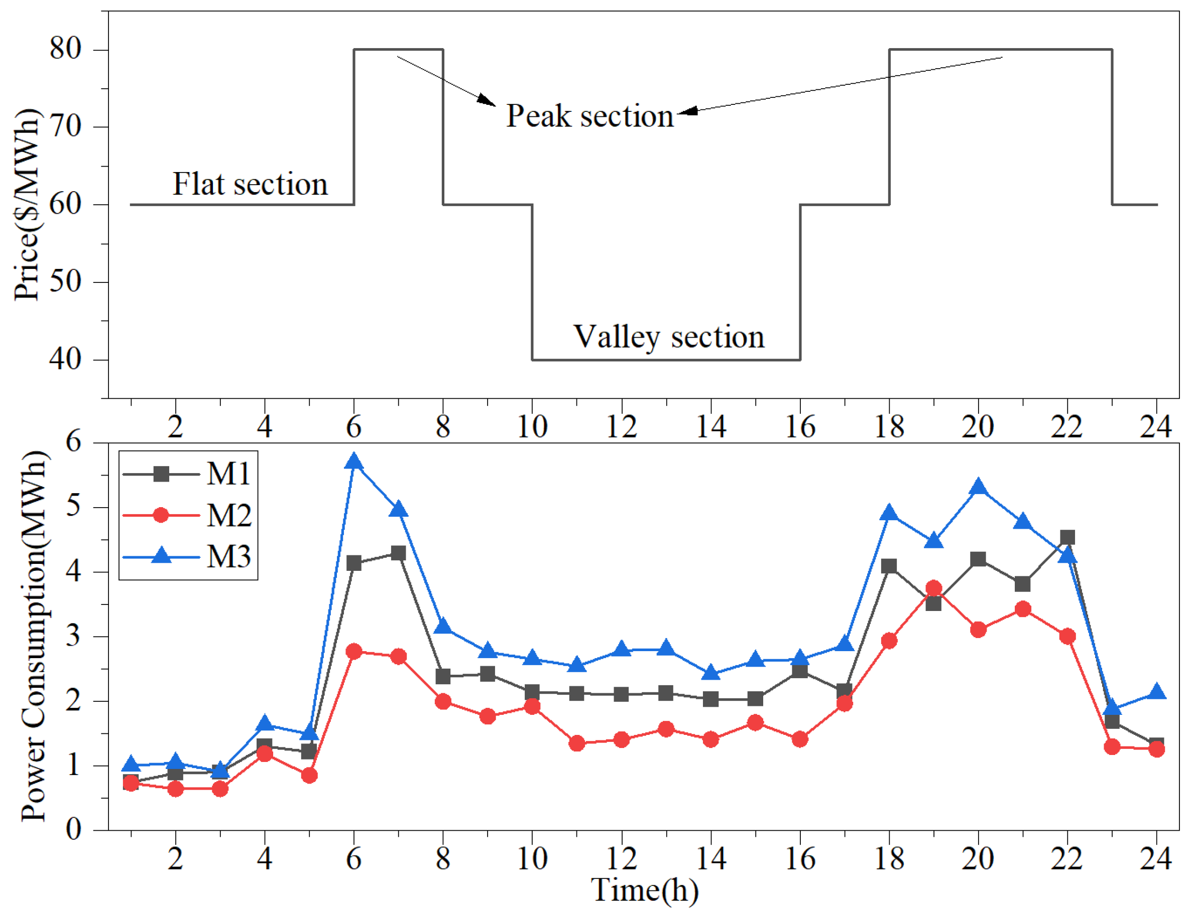
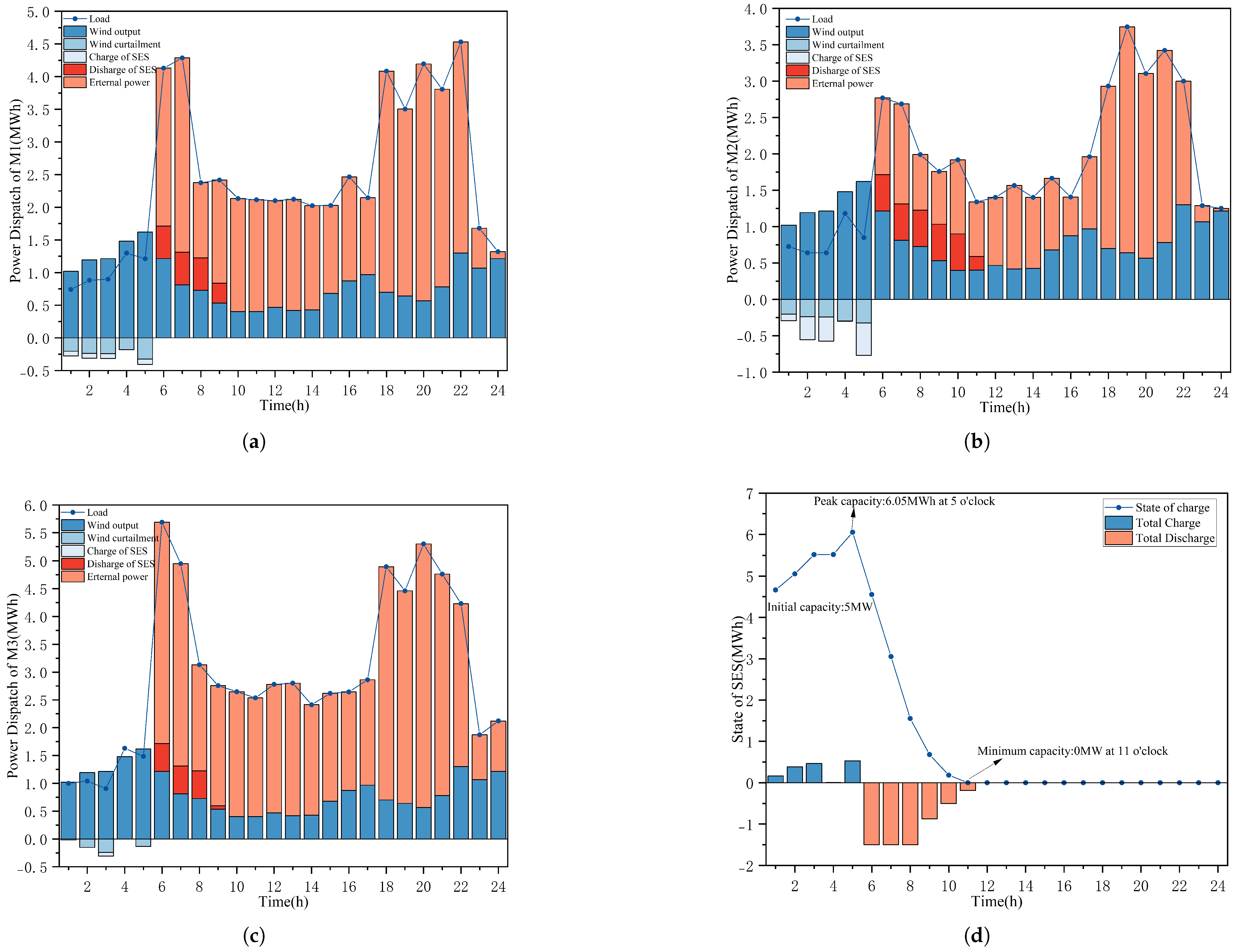
5.1. System Data and Analysis of Results

The system structure aligns with that shown in Figure 1. Specifically, the community microgrid includes three individual microgrids labeled $M1$, $M2$, and $M3$, each containing renewable energy generation units and corresponding loads. Since they are located within the same community, the forecasted and actual renewable energy outputs are identical across the three microgrids. For convenience, the renewable energy is assumed to be wind power. Additionally, the community has an SES unit connected to all three microgrids. All three microgrids are connected to the external grid to ensure power supply reliability.

The forecasted renewable energy output is based on processed data from a wind farm in northwest China [35], with forecast errors assumed to follow a Gaussian distribution. The external grid electricity price adopts a basic time-of-use pricing model, including peak, flat, and valley periods [36]. The predicted and actual output data of wind power and the corresponding prediction errors, which were obtained from Shaanxi Province on 23 October 2023, are shown in Figure 5. The weather was sunny that day, with a wind speed of about 3.5 m/s, and the corresponding wind turbine diameter was about 80 m. The external grid electricity prices are shown in Figure 6. The maximum capacity of SES was set to 10 MWh, and other parameters in the system are illustrated in

Table 2. Values of parameters in test system.

Unit	Price.peak	Price.flat	Price.valley	$\gamma$	$C_{SES}$ [37]	$\overline{g_i^t}$
Value	80 USD/MWh	60 USD/MWh	40 USD/MWh	60 USD/MWh	4 USD/MWh	200 MW
Unit	$\overline{{\omega }_i^t}$	$\overline{p_{i,dis}}$	$\overline{p_{i,chs}}$	$\overline{{\omega }_{i,cur}^t}$ / ${\omega }_i^t$	$\eta$ [37]	$\overline{E}$
Value	5 MW	0.5 MW	0.5 MW	0.5	0.9	10 MWh

. The numerical study was performed on a computer with Intel Core i5-12400F and 32G RAM, and the optimization problem was solved by GUROBI 10.0.2. The optimization results of the system with $\rho =\delta =0.05$ for a data set with 600 samples are shown in Figure 7.

From the first three subfigures in Figure 7, we can observe that during the period from 0 to 5 h, when the wind power output is higher than the electricity demand, the load of each microgrid can be fully supplied by wind power. Additionally, surplus electricity can be used to charge the SES and even produce a small amount of wind power curtailment. Starting from 6 h, the wind power output is lower than the electricity demand. In this case, besides consuming the electricity stored in the SES by discharging, external electricity needs to be purchased to compensate for the electricity gap between supply and demand. Figure 7d, which shows the state of SES, also reflects that the capacity is replenished through charging from 0 to 5 h and then rapidly discharged until it is depleted. The initial capacity is 5 MW. From 0 to 5 h, the capacity of the SES quickly rises to its maximum value of 6.05 MW as each microgrid charges the SES and consumes its surplus power. Subsequently, the wind output cannot afford the loads due to the increase in the microgrid’s load. Due to the marginal cost of SES being lower than the price of purchasing electricity from the external power grid, energy storage is dispatched first so that the SES discharges and its capacity is rapidly consumed until it drops to 0.

5.2. Benchmarks and Evaluation Metrics

We use the above system to test the proposed approach, while several commonly used optimization methods are chosen for comparison:

(1)

The optimal baseline (OPT): OPT refers to deterministic optimization without forecast errors, where it is assumed that the output of renewable energy can be perfectly predicted, thereby achieving the optimal electricity cost.

(2)

Chance-constrained optimization (CC): The CC method is used for comparison, and it is assumed that the forecast errors of renewable energy output follow a Gaussian distribution.

(3)

Scenario generation (SG): SG represents uncertainty using a set of scenarios, and is also a commonly used stochastic optimization method [38,39]. Several renewable energy output scenarios are set up for comparative analysis.

(4)

Sample-based robust optimization (SRO): SRO is the proposed robust optimization approach based on the concept of statistical feasibility. The uncertainty set is constructed solely from the samples.

(5)

Reconstructed sample-based RO (RSRO): RSRO is the approach proposed in this study, which performs robust optimization based on samples and reconstructed uncertainty sets.

To evaluate the performance of the aforementioned optimization approaches, we performed 100 trials for each set of samples and focused on two indicators, the effectiveness of the optimization objective and the probability of constraint violations during the optimization process, which are represented by the cost increase (CI) and the average constraint violation rate (ACVR), respectively. Specifically, CI refers to the percentage increase in the objective function value of other methods compared to the optimal value obtained by the OPT method. ACVR represents the probability of constraint violations after multiple sample tests. The details are as follows:

$$CI={\displaystyle \frac{obj-ob{j}^{*}}{ob{j}^{*}}}$$

(34)

$$ACVR={\mathbb{E}}_{D_{\xi }}\left[\mathbb{P}\left(\mathrm{H}\left(\widehat{\mathbf{a}}(i,t),{\xi }_i^t\right)>\overline{{\omega }_{i,cur}^t}\right)\right]={\displaystyle \frac{1}{100n}}\sum _{D_{\xi }}\sum _{\xi }{I}_{vio}(D_{\xi },\xi )$$

(35)

where $obj$ denote the objective value of each optimization approach, while $ob{j}^{*}$ refers to the objective value of OPT. $I_{vio}(D_{\xi },\xi )$ is the indicator function, whose value is 1 when $\mathrm{H}\left(\widehat{\mathbf{a}}(i,t),{\xi }_i^t\right)>\overline{{\omega }_{i,cur}^t}$, and otherwise, it is 0.

The numerical studies were conducted with an initial setting of $\rho =\delta =0.05$ and a sample size of 600.

Table 3. Performance of different approaches ($\rho =\delta =0.05, n=600$).

Approach	OPT	CC	SG	SRO	RSRO
Cost(USD)	1257.66	1342.18	1392.61	1425.43	1393.74
CI(%)	0	6.72	10.73	13.34	10.82
ACVR	0	0.0529	0.0275	0.024	0.0419

shows the values of the main parameters obtained. We can see that CC achieves the optimal solution closest to OPT but does not meet the ACVR requirement, making the solution infeasible. The other three approaches all produce feasible solutions, with SG yielding the best results, and RSRO’s ACVR is closest to 0.05.

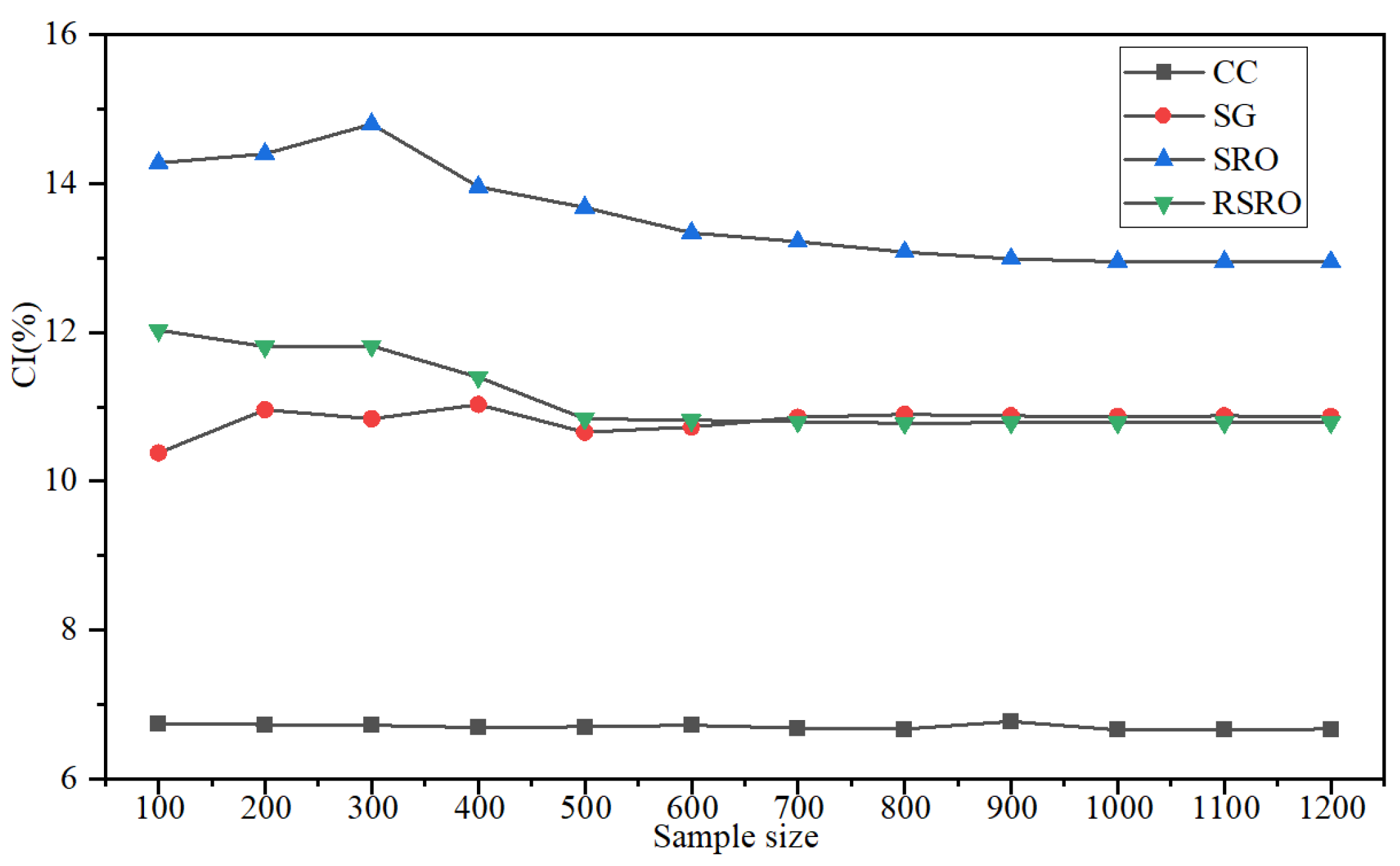
5.3. Performance Analysis with Varying Sample Sizes

The sample size reflects the distribution information of uncertain parameters, thereby influencing the performance of different optimization approaches. To investigate the change in CI and ACVR obtained by the above approaches at different sample sizes, we chose different sample sets and conduct tests under $\rho =\delta =0.05$. The objectives obtained by different approaches under different sample sizes are illustrated in

Table 4. Objectives under different sample sizes ($\rho =\delta =0.05$, the cost of OPT is USD 1257.66).

Size	CC (USD)	SG (USD)	SRO (USD)	RSRO (USD)
100	1342.42	1388.21	1437.25	1408.96
200	1342.30	1395.50	1348.76	1406.19
300	1342.18	1393.99	1443.79	1406.32
400	1341.80	1396.38	1433.23	1401.03
500	1341.92	1391.73	1429.71	1393.99
600	1342.18	1392.61	1425.43	1393.74
700	1341.67	1394.24	1423.92	1393.49
800	1341.55	1394.75	1422.16	1393.24
900	1342.80	1394.49	1421.03	1393.30
1000	1341.42	1394.37	1420.53	1393.32
1100	1341.29	1394.49	1420.28	1393.24
1200	1341.55	1394.39	1420.33	1393.46

, and comparisons of the CI and ACVR values are presented in Figure 8 and Figure 9.

As shown in Figure 8, the optimization results obtained by CC are better than those of other approaches, and it is almost unaffected by the sample size. The results obtained by SG are second only to to those obtained by CC. When the sample size is less than 600, the results obtained by SG outperform RSRO’s. However, as the sample size increases, the difference between SG and RSRO becomes negligible. Additionally, the results of SRO are the most conservative due to the inherent conservatism of RO methods. On the other hand, RSRO significantly outperforms SRO, as the reconstruction of the uncertainty set enhances the performance of the optimization approach and reduces its conservatism. Moreover, from Figure 9, we can observe that the optimization results of CC based on Gaussian distribution consistently fail to meet the stability requirements of the sample set (the curve of ACVR is above the given stability requirement curve, indicated by the gray line). This could be due to the assumption that Gaussian distribution does not accurately capture the characteristics of the sample set, highlighting the significant influence of the distribution characteristics on the performance of the CC method. The results of the other three approaches remain feasible throughout. Among them, the ACVR of SG shows a decreasing trend as the sample size increases, indicating that the larger sample size brings more constraints and reduces the likelihood of constraint violations in SG. SRO and RSRO show similar trends in their ACVRs, which increase as the sample size grows. However, it is noteworthy that the ACVR of RSRO tends to approach the gray curve more closely, suggesting that RSRO can better utilize the stability requirements and thus has the potential to yield superior optimization results.

Based on the above analysis, CC based on Gaussian distribution yields the best result, but it is always infeasible under the given stability requirements. SG can provide good results while satisfying the stability requirements. Regarding the optimization results and constraint violation levels, RSRO outperforms SRO significantly. Moreover, compared to the other three approaches, RSRO can best utilize the stability requirements while reducing the conservatism of robust optimization, and this performance is more apparent when the sample size is more significant.

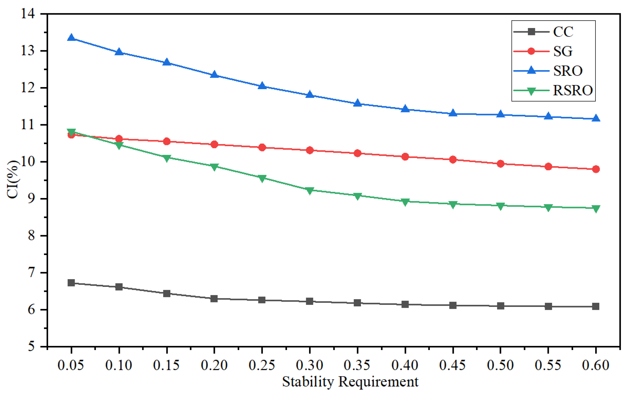
5.4. Performance Analysis with Varying Constraint Stability Requirements

In this subsection, we investigate the performance of different approaches as the stability requirement changes. To eliminate the impact of sample size, we fix the sample size at 600. The objectives of different approaches when the stability requirement varies between 0.05 and 0.6 are shown in

Table 5. Objectives under different stability requirements ($n=600$, the cost of OPT is USD 1257.66).

Stability Requirement ($\mathit{\rho }$)	CC (USD)	SG (USD)	SRO (USD)	RSRO (USD)
0.05	1342.18	1392.61	1425.43	1393.74
0.10	1340.79	1391.22	1420.65	1389.21
0.15	1338.65	1390.34	1417.13	1384.94
0.20	1336.89	1389.34	1412.86	1381.92
0.25	1336.39	1388.33	1409.08	1378.02
0.30	1335.89	1387.33	1406.06	1373.87
0.35	1335.38	1386.32	1403.17	1371.98
0.40	1334.88	1385.18	1401.29	1369.97
0.45	1334.63	1384.18	1399.78	1369.09
0.50	1334.38	1382.80	1399.40	1368.59
0.55	1334.26	1381.93	1398.77	1368.08
0.60	1334.13	1380.91	1398.02	1367.71

, and the corresponding performance values are detailed in Figure 10 and Figure 11.

Firstly, from Figure 10, it can be observed that the optimization results of different approaches follow a similar trend to the stability requirement changes. The higher the stability requirement, the better the optimization results. When the stability requirement is around 0.05, the SG results are better than RSRO’s. However, as $\rho$ increases, the performance of RSRO improves rapidly and soon surpasses that of SG. When the stability requirement exceeds 0.1, RSRO consistently provides the second-best results after CC. Furthermore, Figure 11 shows that the ACVR of all approaches increases as the stability requirement increases. Specifically, CC still fails to obtain a feasible solution under the given stability requirements, with its ACVR curve consistently above the stability requirement line. The other three approaches, SG, RSO, and RSRO, produce feasible solutions under different stability requirements. Among them, RSRO shows the most significant variation with changes in the stability requirement, followed by RSO, while SG exhibits the least variation. The ACVR of RSRO remains consistently close to the given stability requirement curve.

In summary, although Gaussian-based CC can achieve the best results under different stability requirements, it cannot guarantee feasibility under the given sample set. In contrast, the proposed RSRO approach can effectively utilize the stability requirement to solve optimization problems with uncertainty, demonstrating better performance than SG and SRO.

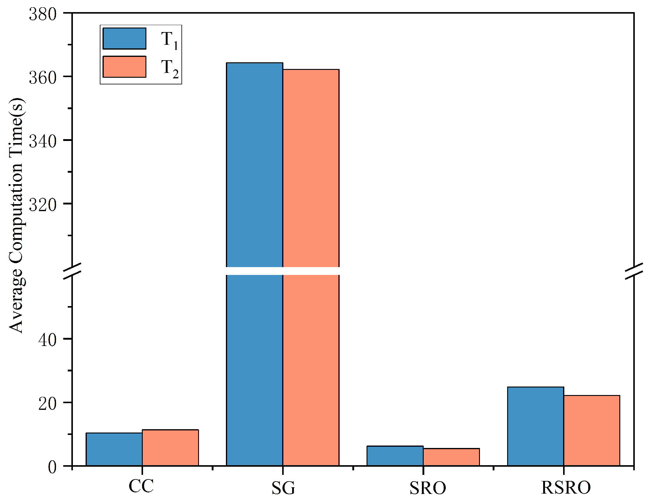
5.5. Evaluation of Computation Time

We also recorded the computation times in the tests conducted in Section 5.3 and Section 5.4. Due to the large number of tests, the average computation time under different sample sizes in Section 5.3 is denoted as $T_1$ for comparison. In contrast, the average computation time under different stability requirements in Section 5.4 is $T_2$. The results are shown in Figure 12. In addition, the computation time of SG varies significantly with the sample size, which is summarized in

Table 6. Calculation time of SG under different sample sizes.

n	100	200	300	400	500	600
Time (s)	125.87	175.39	226.84	273.16	322.16	364.28
n	700	800	900	1000	1100	1200
Time (s)	417.95	461.39	559.85	606.24	662.38	712.36

.

Intuitively, as shown in Figure 12, the computation time of SG is significantly higher than that of the other approaches. In fact, SG needs to generate many scenarios to ensure the statistical significance’s reliability, which will slow down the calculation process. At the same time, the increase in sample size will bring more constraints, which will also extend the calculation time. RSRO, on the other hand, can centrally express a large number of sample constraints in the form of uncertainty sets, which can reduce the complexity of the problem and thus reduce the computation time compared to SG.

Table 6 shows that the computation time of SG increases as the sample size grows, with a nearly linear relationship between them. The computation times of SRO and CC are similar. However, since the iterative process of RSRO is roughly twice as long as that of SRO, the computation time of RSRO is more than twice that of SRO.

6. Conclusions

In this paper, we first establish a community model with multiple microgrids equipped with SES and construct a deterministic optimization model to minimize community electricity costs. Considering the uncertainty in renewable energy output forecasts, we transform the problem into a CCO model to control the curtailment ratio. Furthermore, by introducing the concept of statistical feasibility, we convert the problem into SRO. Specifically, the construction of the uncertainty set involves two steps: shape learning and size calibration. To reduce the conservatism of the optimization results, we incorporate constraint characteristics to perform uncertainty set reconstruction and transform the problem into RSRO, for which the solution methodology is customized. The following findings can be summarized from numerical studies:

• The SES is charged from 0 to 5 h and discharged from 6 h until its capacity drops to 0. The peak capacity of SES reaches 6.05 MWh at 5 h.
• The proposed approach is compared with traditional methods like CC and SG. The results show that the SRO and RSRO approaches can obtain a 13.34% and 10.82% cost increase compared to OPT when $\rho =\delta =0.05, n=600$.
• The proposed RSRO approach can maximize the utilization of the stability requirements of the optimization problem and can effectively reduce the conservatism of SRO. Meanwhile, the relatively low computational time ensures the efficiency of the proposed approach.

In future research, we will consider the life-span cost of SES and examine more sources of uncertainty to expand the profit space of SES based on achieving optimal dispatch.

References

1. Wang, D.; Liu, N.; Chen, F.; Wang, Y.; Mao, J. Progress and prospects of energy storage technology research: Based on multidimensional comparison. J. Energy Storage 2024, 75, 109710. [Google Scholar] [CrossRef]
2. Hu, J.; Wang, Y.; Dong, L. Low carbon-oriented planning of shared energy storage station for multiple integrated energy systems considering energy-carbon flow and carbon emission reduction. Energy 2024, 290, 130139. [Google Scholar] [CrossRef]
3. Wang, W.; Yuan, B.; Sun, Q.; Wennersten, R. Application of energy storage in integrated energy systems—A solution to fluctuation and uncertainty of renewable energy. J. Energy Storage 2022, 52, 104812. [Google Scholar] [CrossRef]
4. Reza, M.; Hannan, M.; Ker, P.J.; Mansor, M.; Lipu, M.H.; Hossain, M.; Mahlia, T.I. Uncertainty parameters of battery energy storage integrated grid and their modeling approaches: A review and future research directions. J. Energy Storage 2023, 68, 107698. [Google Scholar] [CrossRef]
5. Garcia-Torres, F.; Bordons, C.; Tobajas, J.; Real-Calvo, R.; Santiago, I.; Grieu, S. Stochastic optimization of microgrids with hybrid energy storage systems for grid flexibility services considering energy forecast uncertainties. IEEE Trans. Power Syst. 2021, 36, 5537–5547. [Google Scholar] [CrossRef]
6. Zhong, W.; Xie, K.; Liu, Y.; Xie, S.; Xie, L. Chance constrained scheduling and pricing for multi-service battery energy storage. IEEE Trans. Smart Grid 2021, 12, 5030–5042. [Google Scholar] [CrossRef]
7. Jiang, W.; Lu, C.; Wu, C. Robust scheduling of thermostatically controlled loads with statistically feasible guarantees. IEEE Trans. Smart Grid 2023, 14, 3561–3572. [Google Scholar] [CrossRef]
8. Bayram, I.S.; Abdallah, M.; Tajer, A.; Qaraqe, K.A. A Stochastic Sizing Approach for Sharing-Based Energy Storage Applications. IEEE Trans. Smart Grid 2017, 8, 1075–1084. [Google Scholar] [CrossRef]
9. Dai, R.; Charkhgard, H.; Rigterink, F. A robust biobjective optimization approach for operating a shared energy storage under price uncertainty. Int. Trans. Oper. Res. 2022, 29, 1627–1658. [Google Scholar] [CrossRef]
10. Han, O.; Ding, T.; Zhang, X.; Mu, C.; He, X.; Zhang, H.; Jia, W.; Ma, Z. A shared energy storage business model for data center clusters considering renewable energy uncertainties. Renew. Energy 2023, 202, 1273–1290. [Google Scholar] [CrossRef]
11. Liu, D.; Cao, J.; Liu, M. Joint Optimization of Energy Storage Sharing and Demand Response in Microgrid Considering Multiple Uncertainties. Energies 2022, 15, 3067. [Google Scholar] [CrossRef]
12. Wang, Q.; Zhang, X.; Yi, C.; Li, Z.; Xu, D. A Novel Shared Energy Storage Planning Method Considering the Correlation of Renewable Uncertainties on the Supply Side. IEEE Trans. Sustain. Energy 2022, 13, 2051–2063. [Google Scholar] [CrossRef]
13. Zeng, L.; Gong, Y.; Xiao, H.; Chen, T.; Gao, W.; Liang, J.; Peng, S. Research on interval optimization of power system considering shared energy storage and demand response. J. Energy Storage 2024, 86, 111273. [Google Scholar] [CrossRef]
14. Mehrjerdi, H.; Iqbal, A.; Rakhshani, E.; Torres, J.R. Daily-seasonal operation in net-zero energy building powered by hybrid renewable energies and hydrogen storage systems. Energy Convers. Manag. 2019, 201, 112156. [Google Scholar]
15. Si, S.; Sun, W.; Wang, Y. A decentralized dispatch model for multiple micro energy grids system considering renewable energy uncertainties and energy interactions. J. Renew. Sustain. Energy 2024, 16, 015301. [Google Scholar]
16. Lu, Y.; Alghassab, M.; Alvarez-Alvarado, M.S.; Gunduz, H.; Khan, Z.A.; Imran, M. Optimal distribution of renewable energy systems considering aging and long-term weather effect in net-zero energy building design. Sustainability 2020, 12, 5570. [Google Scholar] [CrossRef]
17. Mohammadi, F.; Faghihi, F.; Kazemi, A.; Salemi, A.H. The effect of multi-uncertainties on battery energy storage system sizing in smart homes. J. Energy Storage 2022, 52, 104765. [Google Scholar]
18. Walker, A.; Kwon, S. Design of structured control policy for shared energy storage in residential community: A stochastic optimization approach. Appl. Energy 2021, 298, 117182. [Google Scholar] [CrossRef]
19. Huang, Y.; Wang, L.; Guo, W.; Kang, Q.; Wu, Q. Chance Constrained Optimization in a Home Energy Management System. IEEE Trans. Smart Grid 2018, 9, 252–260. [Google Scholar] [CrossRef]
20. Njema, G.G.; Ouma, R.B.O.; Kibet, J.K. A review on the recent advances in battery development and energy storage technologies. J. Renew. Energy 2024, 2024, 2329261. [Google Scholar]
21. Liang, Z.; Chen, H.; Chen, S.; Wang, Y.; Zhang, C.; Kang, C. Robust Transmission Expansion Planning Based on Adaptive Uncertainty Set Optimization Under High-Penetration Wind Power Generation. IEEE Trans. Power Syst. 2021, 36, 2798–2814. [Google Scholar] [CrossRef]
22. Ben-Tal, A.; Nemirovski, A. Robust convex optimization. Math. Oper. Res. 1998, 23, 769–805. [Google Scholar]
23. Li, Y.; Hu, W.; Zhang, F.; Li, Y. Collaborative operational model for shared hydrogen energy storage and park cluster: A multiple values assessment. J. Energy Storage 2024, 82, 110507. [Google Scholar] [CrossRef]
24. Siqin, Z.; Niu, D.; Li, M.; Gao, T.; Lu, Y.; Xu, X. Distributionally robust dispatching of multi-community integrated energy system considering energy sharing and profit allocation. Appl. Energy 2022, 321, 119202. [Google Scholar] [CrossRef]
25. Agra, A.; Rodrigues, F. Distributionally robust optimization for the berth allocation problem under uncertainty. Transp. Res. Part B Methodol. 2022, 164, 1–24. [Google Scholar] [CrossRef]
26. Hong, L.J.; Huang, Z.; Lam, H. Learning-based robust optimization: Procedures and statistical guarantees. Manag. Sci. 2021, 67, 3447–3467. [Google Scholar] [CrossRef]
27. Lu, C.; Gu, N.; Jiang, W.; Wu, C. Sample-adaptive robust economic dispatch with statistically feasible guarantees. IEEE Trans. Power Syst. 2023, 39, 779–793. [Google Scholar]
28. Hastie, T.; Tibshirani, R.; Friedman, J. The Elements of Statistical Learning: Data Mining, Inference, and Prediction; Springer: Berlin/Heidelberg, Germany, 2017. [Google Scholar]
29. Ben-Tal, A.; Nemirovski, A. Robust optimization–methodology and applications. Math. Program. 2002, 92, 453–480. [Google Scholar] [CrossRef]
30. Campi, M.C.; Garatti, S. The Exact Feasibility of Randomized Solutions of Uncertain Convex Programs. SIAM J. Optim. 2008, 19, 1211–1230. [Google Scholar] [CrossRef]
31. Kleywegt, A.J.; Shapiro, A.; Homem-de Mello, T. The sample average approximation method for stochastic discrete optimization. SIAM J. Optim. 2002, 12, 479–502. [Google Scholar]
32. Pagnoncelli, B.K.; Ahmed, S.; Shapiro, A. Sample average approximation method for chance constrained programming: Theory and applications. J. Optim. Theory Appl. 2009, 142, 399–416. [Google Scholar] [CrossRef]
33. Boyd, S.; Vandenberghe, L. Convex Optimization; Cambridge University Press: Cambridge, UK, 2004. [Google Scholar]
34. Arroyo, J.M. Bilevel programming applied to power system vulnerability analysis under multiple contingencies. IET Gener. Transm. Distrib. 2010, 4, 178–190. [Google Scholar] [CrossRef]
35. Fang, W.; Yang, C.; Liu, D.; Huang, Q.; Ming, B.; Cheng, L.; Wang, L.; Feng, G.; Shang, J. Assessment of Wind and Solar Power Potential and Their Temporal Complementarity in China’s Northwestern Provinces: Insights from ERA5 Reanalysis. Energies 2023, 16, 7109. [Google Scholar] [CrossRef]
36. Zeng, S.; Li, J.; Ren, Y. Research of time-of-use electricity pricing models in China: A survey. In Proceedings of the 2008 IEEE International Conference on Industrial Engineering and Engineering Management, IEEE, Singapore, 8–11 December 2008; pp. 2191–2195. [Google Scholar]
37. Mitali, J.; Dhinakaran, S.; Mohamad, A. Energy storage systems: A review. Energy Storage Sav. 2022, 1, 166–216. [Google Scholar] [CrossRef]
38. Ma, X.Y.; Sun, Y.Z.; Fang, H.L. Scenario generation of wind power based on statistical uncertainty and variability. IEEE Trans. Sustain. Energy 2013, 4, 894–904. [Google Scholar] [CrossRef]
39. Yan, R.; Wang, J.; Huo, S.; Qin, Y.; Zhang, J.; Tang, S.; Wang, Y.; Liu, Y.; Zhou, L. Flexibility improvement and stochastic multi-scenario hybrid optimization for an integrated energy system with high-proportion renewable energy. Energy 2023, 263, 125779. [Google Scholar] [CrossRef]
Figure 1. The system structure.
Energies 18 01828 g001
Figure 2. Explanation of uncertainty in the system.
Energies 18 01828 g002
Figure 3. Prediction error decomposition.
Energies 18 01828 g003
Figure 4. Formulation of problem and modeling process of SRO and RSRO.
Energies 18 01828 g004
Figure 5. Wind output and prediction errors.
Energies 18 01828 g005
Figure 6. Time-of-use price and power consumption of each microgrid.
Energies 18 01828 g006
Figure 7. Optimization results of the test system. (a) Energy dispatch of M1; (b) energy dispatch of M2; (c) energy dispatch of M3; (d) state of SES.
Energies 18 01828 g007
Figure 8. CI under different sample sizes.
Energies 18 01828 g008
Figure 9. ACVR under different sample sizes.
Energies 18 01828 g009
Figure 10. CI under different stability requirements.
Energies 18 01828 g010
Figure 11. ACVR under different stability requirements.
Energies 18 01828 g011
Figure 12. Average computation time of different approaches.
Energies 18 01828 g012