Optimal Scheduling of Electric Vehicles for Peak Load Regulation: A Multi-Time Scale Approach with Comprehensive Evaluation and Feedback

Abstract

With the increasing prevalence of electric vehicles (EVs), optimizing their scheduling for grid peak-shaving has become a focal point of research. This study develops a multi-time-scale optimization model for EV clusters to participate in peak shaving, integrating a comprehensive evaluation and feedback mechanism. The innovation of this paper lies in the addition of an evaluation and feedback loop to the multi-time-scale scheduling optimization method for EVs participating in peak shaving, which fully utilizes the scheduling potential of EV clusters and mitigates the impact of uncertainties associated with EV clusters. The multi-time-scale approach mitigates response errors stemming from EV uncertainties. A feedback loop enables the grid to adaptively adjust scheduling commands to match real-time conditions. Simulations on the IEEE 33-node system demonstrate that the proposed model effectively optimizes EV load profiles, reducing the peak-to-valley difference rate from 41.74% to 35.19%. It also enhances response accuracy to peak-shaving instructions and upgrades the peak-shaving evaluation from a C rating to a B rating, ultimately increasing the revenue for aggregators participating in peak shaving.

1. Introduction

In recent years, China has prioritized the development of the electric vehicle (EV) industry [1], which has significantly accelerated the adoption and proliferation of EVs. Consequently, the number of EVs has increased rapidly. With the large-scale integration of EV clusters into the power grid, their unregulated charging behavior can increase the control difficulty of the power grid [2] and negatively impact the stability of the power system and voltage quality [3,4,5]. However, EVs can serve as a flexible distributed resource, providing considerable peak-shaving potential for the power grid if aggregated and managed through demand-side response [6,7]. Currently, China is in an important phase of EV industry development, and the issue of how to guide the accurate response of EV clusters to the grid’s peak-shaving instructions is urgent to solve. Researching the schedulable potential of EVs and formulating reasonable peak-shaving instructions and strategies for each charging station within the distribution network is of great significance.

Current research on electric vehicles participating in peak shaving mainly focuses on two aspects: price guidance and direct scheduling. Price guidance leverages demand-side response through time-of-use pricing signals to facilitate EVs for peak shaving and valley filling. Reference [8] sets the peak, valley, and flat periods for the next day with the goal of maximizing the aggregator’s profits and formulates corresponding prices to guide the transfer of EV load. In this context, an aggregator is an entity responsible for integrating and managing multiple distributed energy resources, such as EVs and energy storage systems. Reference [9] combines the topology of the distribution network with traffic flow models to achieve optimal pricing and load migration of the distribution network.

In terms of direct scheduling, reference [10] establishes a multi-objective optimization model with the goals of minimizing the load difference between peaks and valleys and the charging costs of EVs, and formulates the optimal charging strategy for electric vehicles. Reference [11] considers multiple uncertainties and proposes a charging and discharging scheduling model for electric vehicles based on distributionally robust joint chance constraints, effectively balancing cost and reliability.

Single-time-scale scheduling optimization may result in large deviations in the actual scheduling results of EVs. Therefore, some studies use multi-time-scale scheduling optimization methods to ensure more accurate scheduling results for electric vehicles. The multi-time-scale scheduling optimization method is a comprehensive strategy that integrates various time scales. It typically includes day-ahead pre-optimization and intraday rolling optimization. Day-ahead optimization is a 24 h planning strategy that optimizes the system operation plan based on day-ahead load forecasts and renewable energy generation forecasts. Intraday rolling optimization builds on the day-ahead plan, continuously updating the scheduling strategy through a rolling optimization window. It uses short-term forecast information to address forecast errors and scheduling uncertainties [12].

For example, reference [13] proposes a multi-time-scale stochastic optimization scheduling model for electric vehicle charging stations. In the day-ahead stage, the optimization goal is to minimize daily operating costs and optimize the net load curve (the difference between the total system load and the output of distributed renewable energy sources) of the charging station. In the intraday stage, a model predictive control-based intraday rolling optimization is proposed to reduce the impact of insufficient prediction accuracy. Reference [14] establishes a two-layer optimization model, where the upper layer is the system operator who allocates power among aggregators on a rough time scale, and the lower layer is the aggregator who arranges the charging process of individual electric vehicles on a finer time scale to minimize charging costs.

In practical applications, reference [15] proposes a multi-time-scale scheduling method for integrated energy systems (IESs) tailored to the climatic characteristics of long heating periods in the cold regions of Northeast China. This method aims to minimize system operating costs and dynamically adjust equipment output, thereby enhancing the overall efficiency and economic viability of the IES. In a demonstration project of an AC/DC hybrid microgrid, reference [16] employed a multi-time-scale optimization method to reduce daily operating costs and increase the penetration rate of wind and photovoltaic power to 88.74%.

Existing multi-time-scale scheduling optimization models for EV participation in peak shaving can correct response deviations at multiple time scales, enabling charging stations to cope with the uncertainty of EVs in actual responses. However, as the formulator of scheduling instructions, the power grid can only passively accept the final scheduling results. Specifically, existing multi-time-scale scheduling optimization models for EV participation in peak shaving lack an evaluation and feedback mechanism for scheduling results. Consequently, the power grid cannot accurately grasp the actual schedulable potential of EVs and cannot actively and flexibly adjust scheduling strategies according to actual conditions.

To address the absence of evaluation and feedback mechanisms in current EV grid scheduling research, this paper proposes a multi-time-scale closed-loop scheduling model integrating comprehensive evaluation and feedback (“day-ahead pre-optimization—intraday rolling optimization—result feedback”). The main research contributions of this paper are:

(1)

Combining day-ahead price guidance with intraday scheduling to establish a multi-time-scale optimization strategy for EV participation in peak shaving. This strategy not only considers the self-interest of EVs [17] but also meets the grid’s peak-shaving requirements, improving the accuracy of response scheduling.

(2)

Integrating a comprehensive evaluation process into the multi-time-scale method, evaluating the actual peak-shaving effects of EV clusters, determining the remuneration of aggregators participating in peak shaving, and making the entire scheduling transaction process fairer and more objective.

(3)

Feeding back the comprehensive evaluation results to the grid, enabling the grid to actively adjust the peak-shaving instructions for EVs in the next scheduling cycle to adapt to the actual schedulable potential of the EV cluster, and achieving refined management of the scheduling potential of EVs.

The structure of this paper is as follows: Section 1 introduces the research background and current status. Section 2 presents the overall framework of the multi-time-scale optimization scheduling method for electric vehicles participating in peak shaving proposed in this paper. Section 3 elaborates on the day-ahead pre-optimization model in multi-time-scale optimization scheduling. Section 4 details the intraday rolling optimization and evaluation, as well as feedback mechanisms in multi-time-scale optimization scheduling. Section 5 validates the effectiveness of the model through simulations on the IEEE 33-node system and presents numerical results. Section 6 summarizes the relevant conclusions of this paper and discusses the innovations and limitations of the model.

2. Overall Process of Grid Scheduling EVs for Peak Shaving

The overall process is divided into three parts: day-ahead pre-optimization, intraday rolling optimization, and result evaluation and feedback. The technical route is shown in Figure 1.

Day-ahead Stage: The grid formulates peak-shaving instructions with the goals of peak shaving and valley filling. It combines the schedulable potential of each charging station to allocate peak-shaving instructions to the EV aggregators of each charging station, with the goal of minimizing network losses. Each charging station, while ensuring that its own benefits are not reduced, aims to respond to the scheduling instructions to the greatest extent possible and sets electricity prices to guide EVs. The day-ahead scheduling is a 24 h scheduling with a time resolution of 1 h.

Intraday Stage: Each charging station aims to minimize the execution deviation of the grid scheduling instructions. It combines the “remaining schedulable potential—scheduling cost” relationship curve of the electric vehicle cluster and increases additional scheduling costs to adjust EVs to correct deviations. The intraday optimization is a 1 h scheduling with a time scale of 15 min.

Evaluation and Feedback Stage: The final peak-shaving and valley-filling effects are evaluated, and the peak-shaving costs are determined based on the completion effect. The scheduling results are also fed back to the grid as a reference for the next peak-shaving instructions.

3. Day-Ahead Pre-Optimization Model

The day-ahead pre-optimization process consists of two stages. First, the grid formulates and allocates peak-shaving instructions. Second, each charging station optimizes electricity prices to guide the orderly charging and discharging of electric vehicles.

3.1. Formulation and Allocation of Peak-Shaving Instructions

Firstly, the power grid forecasts the load of the distribution network for the next day, denoted as $P_{load}(t)$. The periods during which the load power exceeds the upper limit of safe operation ($P_{max}$) and falls below the lower limit ($P_{min}$) are designated as peak-shaving and valley-filling periods, denoted as $T^{*}$. During these periods, the grid must reduce or fill in the load power that exceeds the acceptable range. Based on this, the grid assigns an overall peak shaving and valley filling target $\alpha (t^{*})$ to the EV aggregators. Here, $\alpha (t^{*}),(0\le \alpha \le 1,t^{*}\in T^{*})$ represents the proportion of the load power reduction or increase that the aggregator’s EV cluster needs to undertake during the period $T^{*}$. The overall peak-shaving and valley-filling target for the aggregator is:

$$P_{ref}(t^{*})=\left\{\begin{array}{l}\alpha (t^{*})·(P_{load}(t^{*})-P_{\max }),P_{load}(t^{*})\ge P_{\max },t^{*}\in T^{*}\\ \alpha (t^{*})·(P_{\min }-P_{load}(t^{*})),P_{load}(t^{*})\le P_{\min },t^{*}\in T^{*}\end{array}\right.$$

(1)

Subsequently, the power grid, in conjunction with the topology of the distribution network and the schedulable potential range of electric vehicles at each charging station within the aggregator, allocates peak-shaving instructions $P_{ref}(t^{*})$ to minimize network losses. The schedulable potential range of electric vehicles at each charging station is derived using the Minkowski sum method from reference [18], yielding parameters that characterize the schedulable potential of the charging station: $P_n^{\mathrm{ch},\max }(t),P_n^{\mathrm{d},\max }(t),$ $\Delta S_n(t),S_n^{\min }(t),S_n^{\max }(t)$. These parameters represent the maximum charging power, maximum discharging power, the change in electricity quantity due to the grid-connected status of the electric vehicle cluster at charging station n during period t, the lower limit of electricity quantity, and the upper limit of electricity quantity, respectively.

3.1.1. Grid Objective Function

To efficiently solve the optimal power flow problem in distribution networks, this paper employs the second-order cone relaxation. This technique transforms the original non-convex optimization problem into a convex one by converting nonlinear constraints into second-order cone constraints. This ensures the existence of a global optimal solution and significantly improves computational efficiency [19].

Based on the second-order cone relaxation calculation of the optimal power flow in distribution networks, the grid’s objective function is to minimize network losses:

$$\min f=\sum _{t=1}^T\sum _{(i,j)\in E}{r}_{ij}·I_{ij}(t)$$

(2)

here, $T$ is the total number of operating periods, $E$ is the set of lines, $(i,j)$ is the line ${\mathcal{l}}_{ij}$, $r_{ij}$ is the resistance of the line, and $I_{ij}(t)$ is the square of the current amplitude of the line ${\mathcal{l}}_{ij}$ during period t. The impedance and admittance between adjacent nodes i and j in the distribution network are represented as: $z_{ij}=r_{ij}+j{x}_{ij}$, $y_{ij}=1/z_{ij}=g_{ij}-j{b}_{ij}$.

3.1.2. Instruction Allocation Constraints

The constraints for instruction allocation are divided into power balance constraints, operational constraints, and charging station load constraints. Let branch ij represent the direction of the power flow from node i to node j; $\delta (j)$ is the set of branch ends with node j as the head node, $\delta (j)$ is the set of branch starts with node j as the end node, and M is the set of nodes.

(1)

Power balance constraints:

$$P_j(t)=\sum _{k\in \delta (j)}{P}_{jk}(t)-\sum _{i\in \pi (j)}\left(P_i(t)-r_{ij}{I}_{ij}(t)\right)+g_j{v}_j(t)$$

(3)

$$P_j(t)=P_j^{\mathrm{L}}(t)+P_n^{EV}(t)+P_n^{ref}(t)$$

(4)

$$Q_j(t)=\sum _{k\in \delta (j)}{Q}_{jk}(t)-\sum _{i\in \pi (j)}\left(Q_{ij}(t)-I_{ij}(t)x_{ij}\right)+b_j{v}_j(t)$$

(5)

$$Q_j(t)=Q_j^{\mathrm{L}}(t)$$

(6)

$$v_i(t)-v_j(t)=2\left(r_{ij}{P}_{ij}(t)+x_{ij}{Q}_i(t)\right)-\left(r_{ij}^2+x_{ij}^2\right)I_{ij}(t)$$

(7)

$$I_i(t)={\displaystyle \frac{P_{ij}^2(t)+Q_i^2(t)}{v_i(t)}}$$

(8)

$$S_{ij}(t)=P_{ij}(t)+j{Q}_{ij}(t)$$

(9)

here, $v_j(t)$ is the square of the voltage magnitude at node j for any $(i,j)\in E$ during period t. $P_j^{\mathrm{L}}(t)$ and $Q_j^{\mathrm{L}}(t)$ are the active and reactive powers of the conventional load at the distribution network node j. $P_n^{EV}(t)$ is the original active power of the electric vehicle cluster at charging station n before scheduling at node j. $P_n^{ref}(t)$ is the peak-shaving indicator allocated to charging station n at node j. If there is no charging station at node j, then $P_j(t)=P_j^{\mathrm{L}}(t)$. $S_{ij}(t)$ is the complex power at the beginning of the line in period t.

(2)

Operational constraints:

$$P_i(t)=U_i(t)\sum _{j=1}^M{U}_j(t)\left(G_{ij}\cos {\theta }_{ij}+B_{ij}\sin {\theta }_{ij}\right)$$

(10)

$$Q_i(t)=U_i(t)\sum _{j=1}^M{U}_j(t)\left(G_{ij}\sin {\theta }_{ij}-B_{ij}\cos {\theta }_{ij}\right)$$

(11)

$$U^{\min }⩽U_i\left(t\right)⩽U^{\max }$$

(12)

$${\theta }^{\min }⩽{\theta }_i⩽{\theta }^{\max }$$

(13)

here, $P_i(t), Q_i(t)$ represents the active and reactive power at node i at time t. $U_i(t), U_j(t)$ represents the voltage magnitudes at nodes i and j. ${\theta }_{ij}$ represents the phase angle difference between nodes i and j.

(3)

Charging station load constraint:

The peak-shaving instruction allocated to the charging station must not exceed the schedulable range of the charging station.

$$-P_n^{d,\max }(t)\le P_n^{EV}(t)+P_n^{ref}(t)\le P_n^{ch,\max }(t)$$

(14)

here, $P_n^{EV}(t)$ represents the original power of the electric vehicle cluster at charging station n before scheduling.

3.2. Optimal Pricing Strategy for Charging Stations

After determining the optimal peak-shaving instructions for each charging station, the charging station employs a Stackelberg game model to optimize the next day’s electricity prices and the charging and discharging power of electric vehicles. This process ensures that the total charging power of all electric vehicles does not decrease while maximizing the guidance of electric vehicles to respond to peak-shaving instructions.

3.2.1. Day-Ahead Upper-Level Charging Station Objective Function

The objective function for charging station n aims to maximize revenue and minimize instruction response error:

$$\max CS\_f_n={\displaystyle \sum _{t=1}^T(P_n^c(t)·C_n^{ch}(t)-P_n^d(t)·C_n^d(t)-P_n^c(t)C_g(t)+P_n^d(t)·C_g(t))}-f_n^{CS}$$

(15)

$$C_n^{ch}(t)=C_g(t)+C_n^{ch,ex}(t)$$

(16)

$$C_n^d(t)=C_g(t)+C_n^{d,ex}(t)$$

(17)

$$f_n^{CS}=\mu {\displaystyle \sum _{t=1}^T{(P_n^{EV}(t)+P_n^{ref}(t)-P_n^c(t)+P_n^d(t))}^2}$$

(18)

here, $P_n^c(t)$ is the charging power of the electric vehicle cluster at charging station n at time t, $P_n^d(t)$ is the discharging power at time t, and $C_g(t)$ is the time-of-use electricity price at time t. $C_n^{ch}(t)$ and $C_n^d(t)$ are the charging and selling prices set by charging station n, composed of the grid electricity price and charging/selling service fees. $C_n^{ch,ex}(t)$ and $C_n^{d,ex}(t)$ are the additional charging and selling service fees of the charging station (while charging stations do not have the authority to change the grid electricity price, they can adjust the service fees to modify the charging and selling prices). $f_n^{CS}$ is the penalty function term to ensure that the charging and discharging powers of charging station n accurately respond to peak shaving instructions, and $\mu$ is the penalty function factor.

3.2.2. Upper-Level Charging Station Constraints

$$C_n^{ch,\min }\le C_n^{ch,ex}(t)\le C_n^{ch,\max }$$

(19)

$${\displaystyle \sum _{t=1}^T{C}_n^{ch,ex}(t)}/T\le C_n^{ch,av}$$

(20)

$$C_n^{d,\min }\le C_n^{d,ex}(t)\le C_n^{d,\max }$$

(21)

$${\displaystyle \sum _{t=1}^T{C}_n^{d,ex}(t)}/T\le C_n^{d,av}$$

(22)

Constraints (19)–(22) limit the upper and lower bounds, as well as the average value of the service fees set by charging station n, to prevent malicious price increases. $C_n^{ch,\min }$$C_n^{ch,\max }$ and $C_n^{d,\min }$$C_n^{d,\max }$ are the upper and lower limits of the charging and selling service fees. $C_n^{ch,av}$ and $C_n^{d,av}$ are the average values of the charging and selling service fees for the entire day.

3.2.3. Day-Ahead Lower-Level EVs Objective Function

The electric vehicles at charging station n can be optimized as a group to minimize charging costs [20]. The objective function for the electric vehicle cluster at charging station n is:

$$\min EV\_f_n={\displaystyle \sum _{t=1}^T(-P_n^c(t)·C_n^{ch}(t)+P_n^d(t)·C_n^d(t))}$$

(23)

EV Cluster constraints:

$$0\le P_n^c(t)\le P_n^{\mathrm{ch},\max }(t)$$

(24)

$$0\le P_n^d(t)\le P_n^{\mathrm{d},\max }(t)$$

(25)

$$S_n^{\min }(t)\le S_n(t)\le S_n^{\max }(t)$$

(26)

$$S_n(t)=({\eta }^{\mathrm{c}}{P}_n^c(1)-P_n^d(1)/{\eta }^{\mathrm{d}})\Delta t+\Delta S_n(1),t=1$$

(27)

$$S_n(t)=S_n(t-1)+({\eta }^{\mathrm{c}}{P}_n^c(t)-P_n^d(t)/{\eta }^{\mathrm{d}})\Delta t+\Delta S_n(t),t\in [2,T]$$

(28)

$${\displaystyle \sum _{t=1}^T(P_n^c(t)-P_n^d(t))}\ge {\displaystyle \sum _{t=1}^T(P_n^{EV}(t))}$$

(29)

here, $S_n(t)$ represents the electricity quantity of the cluster at time t. Constraints (24)–(26) ensure that the cluster’s power and electricity quantity are within the schedulable potential range, using the maximum charging power $P_n^{\mathrm{ch},\max }(t)$, maximum discharging power $P_n^{\mathrm{d},\max }(t)$, lower limit of electricity quantity $S_n^{\min }(t)$, and the upper limit of electricity quantity $S_n^{\max }(t)$ from the schedulable potential parameters of charging station n. Constraints (27) and (28) describe the relationship between the cluster’s electricity quantity and power, where ${\eta }^{\mathrm{c}}$ and ${\eta }^{\mathrm{d}}$ are the charging and discharging efficiencies of the cluster, respectively. Constraint (29) ensures that the electric vehicle cluster achieves the expected electricity quantity.

4. Intraday Rolling Optimization and Evaluation Feedback

4.1. Intraday Rolling Optimization

Following the day-ahead optimization, each charging station uses the optimized electricity prices to guide EVs in responding to the grid’s scheduling instructions as effectively as possible. However, on the following day, deviations in response power may occur due to various factors. Therefore, charging stations need to correct these deviations through intraday rolling optimization.

Intraday rolling optimization is performed one hour in advance by directly scheduling the electric vehicle cluster to adjust the charging and discharging power within the time period. The objective function is established to minimize the peak-shaving response deviation:

$$\min CS\_f_{n,in}={\displaystyle \sum _{t\in T_l^{*}}(P_n^{EV}(t)+P_n^{ref}(t))-P_{n,in}^{EV}(t))}$$

(30)

$$P_{n,in}^{EV}=P_{n,in}^c(t)-P_{n,in}^d(t)+\Delta P_{n,in}(t)$$

(31)

here, $P_{n,in}^{EV}(t)$ represents the actual power of the electric vehicle cluster at charging station n during the intraday period. $T_l^{*}$ is the time dimension for intraday optimization, which is the range of the rolling window (set to one hour in this context).

$\Delta P_{n,in}(t)$ is the scheduling correction amount for charging station n at time t, and this value must be within the remaining schedulable potential range of charging station n for the intraday period.

$$\left\{\begin{array}{l}\Delta P_{n,in}(t)\le P_{n,in}^{ch,\max }(t)-P_{n,in}^c(t),\Delta P_{n,in}(t)\ge 0\\ \Delta P_{n,in}(t)\ge P_{n,in}^d(t)-P_{n,in}^{d,\max }(t),\Delta P_{n,in}(t)<0\end{array}\right.$$

(32)

here, $\left\{P_{n,in}^{\mathrm{ch},\max }(t),P_{n,in}^{\mathrm{d},\max }(t),\Delta S_{n,in}(t),S_{n,in}^{\min }(t),S_{n,in}^{\max }(t)\right\}$ is the parameter representing the intraday schedulable potential of the electric vehicle cluster at charging station n within the rolling window range.

Charging stations use the remaining intraday schedulable potential to correct errors. Since this part of the scheduling is not a spontaneous response from individual electric vehicles, charging stations need to invest additional scheduling costs to incentivize electric vehicles to accept scheduling. According to prospect theory [21], the relationship between “remaining schedulable charging/discharging power and scheduling power price per unit” is shown in Figure 2.

The curve in the right graph can be described by the following equation:

$$\Delta P_{n,in}(t)=(P_{n,in}^{ch,\max }(t)-P_{n,in}^c(t))\arctan (m_1{C}_{n,in}(t))$$

(33)

$$\Delta P_{n,in}(t)=(P_{n,in}^d(t)-P_{n,in}^{d,\max }(t))\arctan (m_2{C}_{n,in}(t))$$

(34)

here, $C_{n,in}$ is the scheduling power price per unit for charging station n. According to prospect theory, due to loss aversion, the cluster is more sensitive to the scheduling of remaining charging power. Specifically, when scheduling the same amount of charging and discharging power, the scheduling price per unit for discharging power is higher. Therefore, when $P_{n,in}^d(t)-P_{n,in}^{d,\max }(t)=P_{n,in}^c(t)-P_{n,in}^{ch,\max }(t)$, $m_1>m_2$.

Considering that the scheduling price per unit for the charging station increases with the total amount of scheduled power, the charging station needs to weigh the profitability of participating in peak shaving. When the scheduling price per unit exceeds the average peak-shaving revenue price from historical transactions, the charging station will give up further correcting the error.

$$C_{n,in}(t)\le C_{av}^{peak}$$

(35)

here, $C_{av}^{peak}$ is the average peak-shaving revenue price from historical transactions.

4.2. Comprehensive Evaluation and Feedback

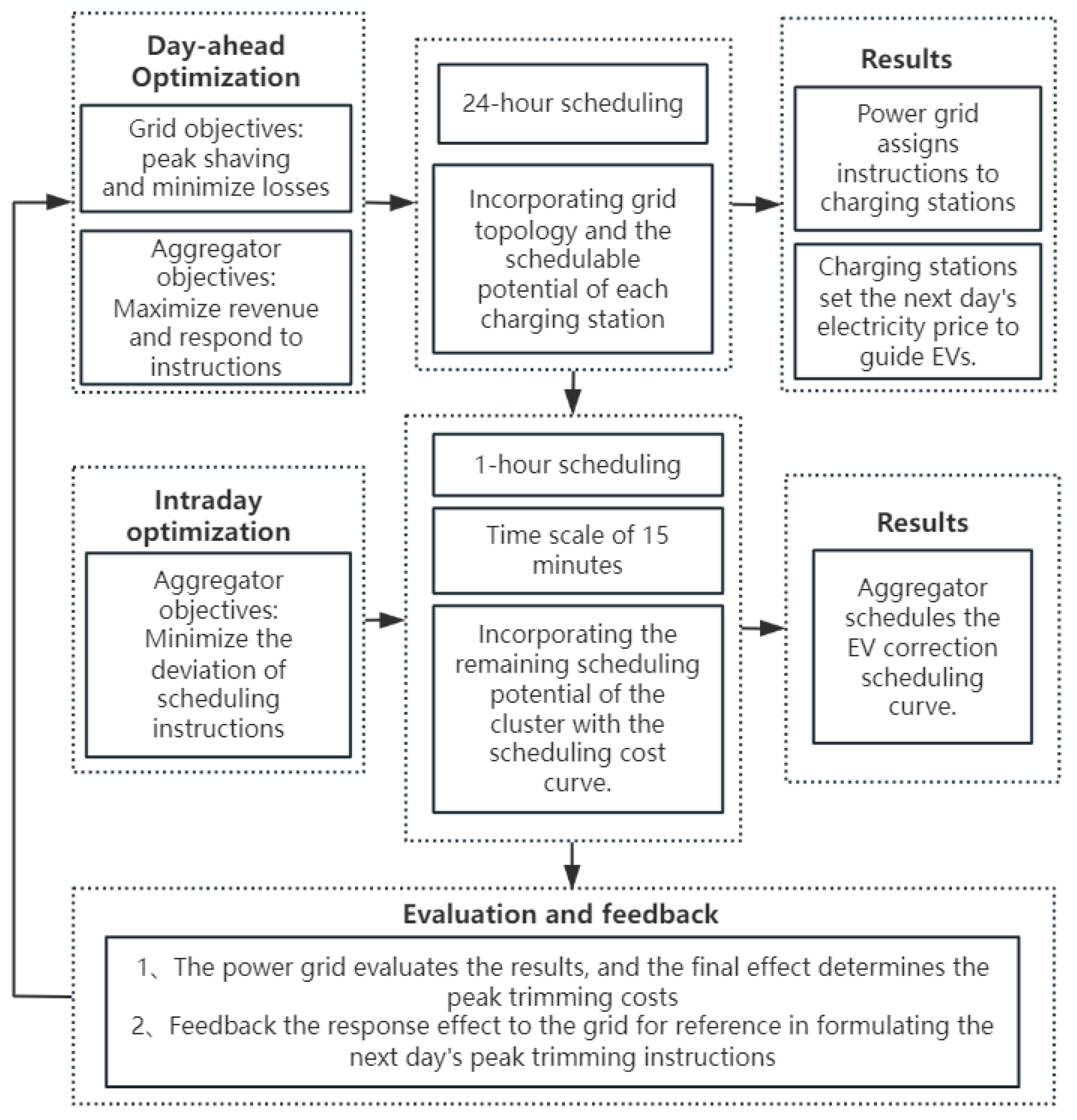
After the peak shaving scheduling is completed, the overall peak-shaving and valley-filling effect of the electric vehicle cluster is evaluated to determine the final unit price. Additionally, the evaluation results are fed back to the power grid, enabling it to promptly and accurately assess the actual response capability of the electric vehicle aggregator. This allows the grid to actively adjust the peak-shaving instructions for the aggregator in subsequent scheduling cycles.

The “average response deviation at each moment, the difference between the maximum and minimum response deviations, the proportion of accurate responses, and the reduction in peak-to-valley difference rate” are selected as the evaluation indicators for the aggregator’s final response effect. The Analytic Hierarchy Process (AHP) is used to determine the weights of different indicators, and then the comprehensive evaluation method of extensible matter elements is used to achieve a quantified comprehensive evaluation and feedback on the peak shaving effect of the electric vehicle aggregator.

The following four metrics are selected as the evaluation indicators for the aggregator’s final response effect: “average response deviation at each moment”, “difference between the maximum and minimum response deviations”, “proportion of accurate responses”, “reduction in peak-to-valley difference rate”.

The Analytic Hierarchy Process (AHP) is used to determine the weights of these indicators. Then, the comprehensive evaluation method of extensible matter elements is used to achieve a quantified comprehensive evaluation and feedback on the peak-shaving effect of the electric vehicle aggregator.

4.2.1. Indicator Classification

The intraday scheduling effect is used as the final peak-shaving result, assuming that the forecast data one hour in advance is accurate and has a negligible error.

(1)

Average response deviation at each moment:

$$x_1={\displaystyle \frac{1}{\left|T^{*}\right|}}{\displaystyle \sum _{t^{*}\in T^{*}}{\displaystyle \sum _{n\in N}({\sigma }_n(t))}}$$

(36)

$${\sigma }_n(t)=\left|P_n^{EV}(t)+P_n^{ref}(t))-P_{n,in}^{EV}(t)\right|$$

(37)

here, N is the set of charging stations, T is the set of peak-shaving and valley-filling periods, and ${\sigma }_n(t)$ is the response deviation of charging station n.

(2)

The difference between the maximum and minimum response deviations:

$$x_2=\max ({\displaystyle \sum _{n\in N}{\sigma }_n(t)})-\min ({\displaystyle \sum _{n\in N}{\sigma }_n(t)})$$

(38)

(3)

Proportion of accurate responses:

$$x_3=\left|T_1^{*}\right|/\left|T^{*}\right|$$

(39)

$$T_1^{*}=\{t\in T^{*}|{\displaystyle \sum _{n\in N}{\sigma }_n(t)}<\sigma \}$$

(40)

here, $\sigma$ is the allowable response error, and $T_1^{*}$ is the set of periods within the allowable response error range.

(4)

Reduction in peak-to-valley difference rate:

$$x_4={\beta }_1-{\beta }_2$$

(41)

$${\beta }_1={\displaystyle \frac{P_{load}^{\max }-P_{load}^{\min }}{P_{load}^{\max }}}$$

(42)

$${\beta }_2={\displaystyle \frac{P_{load,in}^{\max }-P_{load,in}^{\min }}{P_{load,in}^{\max }}}$$

(43)

here, ${\beta }_1$ and ${\beta }_2$ are the peak-to-valley difference rates before and after peak shaving, respectively.

4.2.2. Determining Weights with AHP Hierarchical Analysis Method

Judgment matrix A: The element $a_{ij}$ in the matrix represents the comparison between the indicator in the i-th row and the indicator in the j-th column, quantitatively expressing their relative importance. Specific data are shown in

Table 1. Specific values for judgment matrix construction.

The Importance of Indicator ${\mathit{x}}_{\mathit{i}}$ Relative to Indicator ${\mathit{x}}_{\mathit{j}}$	${\mathit{a}}_{\mathit{i}\mathit{j}}$
equally important	1
slightly more important	3
moderately more important	5
strongly more important	7
extremely important	9

. The specific values of the judgment matrix can be determined by inviting multiple experts from relevant fields to score.

(1)

Determine the indicator weight vector: $M_{\mathrm{i}}={\displaystyle \prod _{\mathrm{j}=1}^4}{\mathrm{a}}_{\mathrm{ij}},\mathrm{i}=1,2,3,4$

(2)

The weight of the i-th indicator is: ${\mathrm{w}}_{\mathrm{i}}={\displaystyle \frac{\sqrt[4]{{\mathrm{M}}_{\mathrm{i}}}}{{\displaystyle \sum _{\mathrm{i}=1}^4}\sqrt[4]{{\mathrm{M}}_{\mathrm{i}}}}}$

Thus, the weight vector of the indicators is: $W=[w_1,w_2,w_3,w_4]$

(3)

Consistency test of the judgment matrix: $CR={\displaystyle \frac{CI}{RI}}$. Generally, if CR < 0.1, the test is considered passed; otherwise, it is not. Here, $CI={\displaystyle \frac{{\lambda }_{\max }-n_x}{n_x-1}}$, where ${\lambda }_{\max }$ is the maximum eigenvalue of the judgment matrix A, $n_x$ is the number of indicators, and the RI value is related to the order of the judgment matrix, as shown in

Table 2. Relationship between RI values and the order of the judgment matrix.

Matrix Order	1	2	3	4	5	6	7	8	9	10
RI	0	0	0.58	0.90	1.12	1.24	1.32	1.41	1.45	1.49

.

4.2.3. Matter–Element Extension Evaluation Method

(1)

Construct the matter–element matrix $\tilde{R}$:

$$\tilde{R}=\left[\begin{array}{ccc}N& I_1& x_1\\ & I_2& x_2\\ & I_3& x_3\\ & I_4& x_4\end{array}\right]$$

(44)

In the formula, N represents the matter–element to be evaluated. $I_1,I_2,I_3,I_4$ represents the evaluation index. $x_1,x_2,x_3,x_4$ represents the specific calculated value of the evaluation index.

(2)

Determine the matter–element matrix for the classical domain $Q_j$ and the node domain $Q_p$:

$${\tilde{R}}_j=\left(\begin{array}{c}{N}_j,I,Q_j\end{array}\right)=\left[\begin{array}{ccc}{N}_j& I_1& Q_{j1}\\ & I_2& Q_{j2}\\ & I_3& Q_{j3}\\ & I_4& Q_{j4}\end{array}\right]=\left[\begin{array}{ccc}{N}_j& I_1& 〈a_{j1},b_{j1}〉\\ & I_2& 〈a_{j2},b_{j2}〉\\ & I_3& 〈a_{j3},b_{j3}〉\\ & I_4& 〈a_{j4},b_{j4}〉\end{array}\right]$$

(45)

In the formula, $N_j$ indicates the j-th level of the rating problem, which is divided into four levels: “A, B, C, D”, hence j = 1, 2, 3, 4. The range of values that the evaluation index $N_j$ takes with respect to the indicators $I_1,I_2,I_3,I_4$ is defined as the classical domain $Q_{j1}$–$Q_{j4}$.

$${\tilde{R}}_p=\left(\begin{array}{c}{N}_p,I,Q_p\end{array}\right)=\left[\begin{array}{ccc}{N}_p& I_1& Q_{p1}\\ & I_2& Q_{p2}\\ & I_3& Q_{p3}\\ & I_4& Q_{p4}\end{array}\right]=\left[\begin{array}{ccc}{N}_p& I_1& 〈a_{p1},b_{p1}〉\\ & I_2& 〈a_{p2},b_{p2}〉\\ & I_3& 〈a_{p3},b_{p3}〉\\ & I_4& 〈a_{p4},b_{p4}〉\end{array}\right]$$

(46)

In the formula, $N_p$ represents the full set of data established for the rating problem. $Q_{p1}$–$Q_{p4}$ is the total range of values that $N_p$ takes with respect to the evaluation indicators $I_1,I_2,I_3,I_4$ and is called the node domain.

In this paper, Level A represents the best performance, while Level D represents the worst. The levels A, B, C and D correspond to I₁, I₂, I₃, I₄ in Equation (46), respectively. The specific threshold selections for the four levels are $〈a_{p1},b_{p1}〉$, $〈a_{p2},b_{p2}〉$, $〈a_{p3},b_{p3}〉$ and $〈a_{p4},b_{p4}〉$.

(3)

Calculate the correlation function: The correlation function indicates the degree of association between the measured values and the various levels within the corresponding index. The correlation function values for the measured values of the index are calculated as in Formulas (47) and (48).

$$K_{ij}=\left\{\begin{array}{c}-{\displaystyle \frac{\rho \left(x_i,Q_{ji}\right)}{\left|Q_{ji}\right|}},\left(x_i\in Q_{ji}\right)\\ {\displaystyle \frac{\rho \left(x_i,Q_{ji}\right)}{\rho \left(x_i,Q_{pi}\right)-\rho \left(x_i,Q_{ji}\right)}},\left(x_i\notin Q_{ji}\cap \rho \left(x_i,Q_{pi}\right)-\rho \left(x_i,Q_{ji}\right)\ne 0\right)\\ -\rho \left(x_i,Q_{ji}\right)-1,\left(x_i\notin Q_{ji}\cap \rho \left(x_i,Q_{pi}\right)-\rho \left(x_i,Q_{ji}\right)=0\right)\end{array}\right.$$

(47)

The distance $\rho \left(x_i,Q_{ji}\right)$ between the actual measured value of the indicator and the classical domain and node domain is given by the following formula:

$$\begin{array}{l}\rho \left(x_i,Q_{ji}\right)=\left|x_i-{\displaystyle \frac{a_{ji}+b_{ji}}{2}}\right|-{\displaystyle \frac{b_{ji}-a_{ji}}{2}}\\ \rho \left(x_i,Q_{pi}\right)=\left|x_i-{\displaystyle \frac{a_{pi}+b_{pi}}{2}}\right|-{\displaystyle \frac{b_{pi}-a_{pi}}{2}}\end{array}$$

(48)

From this, the correlation function moment can be constructed, which represents the degree of association between the actual measured value and the level. Based on this, the correlation function matrix $\tilde{K}$ can be constructed, where $K_{ij}$ indicates the degree of association between the actual measured value of indicator $x_i$ and the level j:

$$\tilde{K}=\left[\begin{array}{ccc}{K}_{11}& \cdots & K_{1j}\\ ⋮& \ddots & ⋮\\ K_{i1}& \cdots & K_{ij}\end{array}\right]$$

(49)

4.2.4. Evaluation Results and Feedback

The overall correlation degree of each indicator can be calculated from the correlation function matrix and the weights of each indicator:

$$F_j=\sum _{i=1}^4{\omega }_i{K}_{ij},j=1,2,3,4$$

(50)

The maximum correlation degree is taken as the final evaluation level of the peak-shaving and valley-filling effect. When the correlation degree is highest, the corresponding evaluation levels are “A, B, C, D”. “A” indicates an excellent peak-shaving effect, and “D” indicates a poor peak-shaving effect.

In addition to the evaluation level, the characteristic value of the level $\underset{\_}{k}$ can be calculated to provide a more detailed quantification of the evaluation results:

$$\underset{\_}{k}={\displaystyle \frac{{\displaystyle \sum _{j=1}^{4}j\overline{F}}}{{\displaystyle \sum _{j=1}^4\overline{F}}}}$$

(51)

$$\overline{F}={\displaystyle \frac{F_j-\min (F_j)}{\max (F_j)-\min (F_j)}}$$

(52)

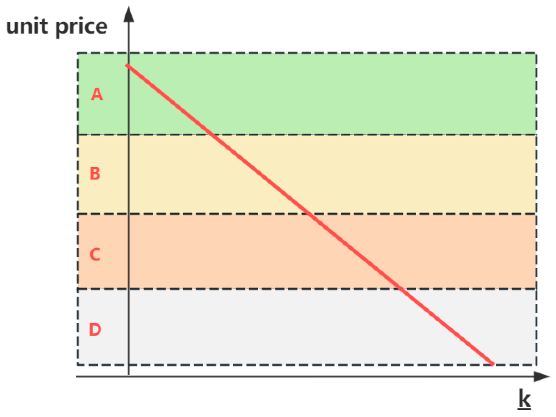
Based on the characteristic value $\underset{\_}{k}$, we can further analyze its tendency to lean toward adjacent levels. The smaller the value of $\underset{\_}{k}$, the better the evaluation effect. Therefore, the characteristic value can be used to determine the final unit price obtained by the charging station. The smaller the value of $\underset{\_}{k}$, the higher the unit price. The relationship curve is shown in Figure 3.

The following expression can be used to describe the situation:

$$C^{peak}=a·\underset{\_}{k}+b$$

(53)

The power grid ultimately rewards the electric vehicle aggregator for peak shaving and valley filling with:

$$C_{all}^{peak}={\displaystyle \sum _{n\in N}{\displaystyle \sum _{t\in T^{*}}\left|P_n^{ref}(t)\right|·}}{C}^{peak}$$

(54)

The general extensible matter–element evaluation method integrates various indicators to determine the evaluation grade. However, to enable the power grid to more accurately analyze the actual scheduling effects, it is necessary to provide feedback on the evaluation grades for individual indicators separately. This allows the power grid to proactively adjust the scheduling strategies for aggregators in the next scheduling cycle, addressing specific issues.

For the evaluation grade of the i-th indicator in the scheduling effect:

$$k_i(j)=\max (F_{i,j}),i=1,2,3,4,j=1,2,3,4$$

(55)

$$F_{i,j}=\sum _{z=1}^4{\omega }_z^{\prime }{K}_{zj},j=1,2,3,4$$

(56)

$${\omega }_z^{\prime }=\left\{\begin{array}{l}1,z=i\\ 0,z\ne i\end{array}\right.$$

(57)

Based on this, we can obtain the evaluation grades for the individual indicators $x_1,x_2,x_3,x_4$ and provide feedback on the evaluation results of these four indicators to the power grid. The grid will then use these results to proactively adjust the scheduling strategies in the next cycle, ensuring that the peak-shaving instructions are more aligned with the actual response capabilities of the electric vehicle cluster. This ultimately leads to the formation of a multi-time-scale closed-loop scheduling system that can continuously adapt to real-world conditions. The detailed adjustment strategies are as follows:

If indicator $x_1$ (average response deviation at each moment) is rated as D, the peak-shaving and valley-filling target $\alpha (t)$ for each period $T^{*}$ is uniformly reduced by $\Delta \alpha (t)$, that is, $\alpha (t)=\alpha (t)-\Delta \alpha (t),(t\in T^{*})$. Conversely, if the result is A, the target is uniformly increased by $\Delta \alpha (t)$, that is, $\alpha (t)=\alpha (t)+\Delta \alpha (t),(t\in T^{*})$.

If the indicator $x_2$ (the difference between the maximum and minimum response deviations) is rated as D, the top 10% of moments with the largest response deviations are identified (denoted as $T_2^{*\prime }$). The peak-shaving and valley-filling target $\alpha (t)$ for each period of $T_2^{*\prime }$ is then uniformly reduced by $\Delta \alpha (t)$, that is, $\alpha (t)=\alpha (t)-\Delta \alpha (t),(t\in T_2^{*\prime })$. Conversely, if the result is A, the top 10% of moments with the smallest response deviations are identified (also denoted as $T_2^{*\prime }$), and the target is uniformly increased by $\Delta \alpha (t)$, that is, $\alpha (t)=\alpha (t)+\Delta \alpha (t),(t\in T_2^{*\prime })$.

If the indicator $x_3$ (the proportion of accurate responses) is rated as D, all moments that exceed the allowed response deviation are identified (denoted as $T_3^{*\prime }$). The peak-shaving and valley-filling target $\alpha (t)$ for each period of $T_3^{*\prime }$ is then uniformly reduced by $\Delta \alpha (t)$, that is, $\alpha (t)=\alpha (t)-\Delta \alpha (t),(t\in T_3^{*\prime })$. Conversely, if the result is A, all moments within the allowed response deviation are identified (also denoted as $T_3^{*\prime }$) and the target is uniformly increased by $\Delta \alpha (t)$, that is, $\alpha (t)=\alpha (t)+\Delta \alpha (t),(t\in T_3^{*\prime })$.

If the indicator $x_4$ (the reduction in peak-valley difference ratio) is rated as D, the top 10% of moments with the highest and lowest distribution network loads are identified (denoted as $T_4^{*\prime }$). The peak-shaving and valley-filling target $\alpha (t)$ for each period of $T_4^{*\prime }$ is then uniformly reduced by $\Delta \alpha (t)$, that is, $\alpha (t)=\alpha (t)-\Delta \alpha (t),(t\in T_4^{*\prime })$. Conversely, if the result is A, then the indicators for $T_4^{*\prime }$ are uniformly increased by $\Delta \alpha (t)$, that is, $\alpha (t)=\alpha (t)+\Delta \alpha (t),(t\in T_4^{*\prime })$.

5. Case Study Verification

5.1. Model Solving

In the multi-time-scale optimization model presented in this paper, the day-ahead scheduling instruction allocation model is a second-order cone programming problem, while the intraday rolling optimization model is a linear programming problem. These models can be directly solved by calling the GUROBI solver via the YALMIP toolbox in MATLAB R2019a.

The day-ahead charging station Stackelberg model, a two-level optimization model, is transformed using the Karush–Kuhn–Tucker (KKT) conditions and dual problems [22]. It is then converted into a mixed-integer linear programming problem (as shown in the formula) and can be solved by GUROBI.

$$\begin{array}{l}\min CS{f}_n={\displaystyle \sum _{t=1}^T[-{\lambda }_n^2(t)P_n^{ch,\max }(t)-{\lambda }_n^4(t)P_n^{d,\max }(t)+{\lambda }_n^5(t)S_n^{\min }(t)-{\lambda }_n^6(t)S_n^{\max }(t)+{\lambda }_n^7(t)\Delta S_n(t)}\\ -P_n^c(t)C_g(t)+P_n^d(t)·C_g(t)]-f_n^{CS}\end{array}$$

(58)

$$\left\{\begin{array}{l}{C}_n^{ch}(t)-{\lambda }_n^1(t)+{\lambda }_n^2(t)-{\lambda }_n^7(t){\eta }^c=0\\ C_n^d(t)-{\lambda }_n^3(t)+{\lambda }_n^4(t)-{\lambda }_n^7(t)/{\eta }^d=0\\ -{\lambda }_n^5(t)+{\lambda }_n^6(t)-{\lambda }_n^7(t)+{\lambda }_n^7(t+1)=0,t\in (1,T-1)\\ -{\lambda }_n^5(t)+{\lambda }_n^6(t)-{\lambda }_n^8(t),t\in (1,T)\end{array}\right.$$

(59)

$$\left\{\begin{array}{l}0\le {\lambda }_n^1(t)\le M{\gamma }_n^1(t),0\le {\lambda }_n^2(t)\le M{\gamma }_n^2(t)\\ 0\le P_n^c(t)\le M[1-{\gamma }_n^1(t)],0\le P_n^{ch,\max }(t)-P_n^c(t)\le M(1-{\gamma }_n^2(t))\\ 0\le {\lambda }_n^3(t)\le M{\gamma }_n^3(t),0\le {\lambda }_n^4(t)\le M{\gamma }_n^4(t)\\ 0\le P_n^d(t)\le M[1-{\gamma }_n^3(t)],0\le P_n^{d,\max }(t)-P_n^d(t)\le M(1-{\gamma }_n^4(t))\\ 0\le {\lambda }_n^5(t)\le M{\gamma }_n^5(t),0\le {\lambda }_n^6(t)\le M{\gamma }_n^6(t)\\ 0\le S_n(t)-S_n^{\min }(t)\le M[1-{\gamma }_n^5(t)],0\le S_n^{\max }(t)-S_n(t)\le M(1-{\gamma }_n^6(t))\end{array}\right.$$

(60)

here, ${\lambda }_n^1(t)-{\lambda }_n^7(t)$ are dual variables, ${\gamma }_n^1(t)-{\gamma }_n^6(t)$ are Boolean variables, and M is a sufficiently large number. For the simulation, the GUROBI solver’s gap value is set to 0.01%.

5.2. Parameter Settings

Simulations are conducted on the IEEE 33-node system, with charging stations located in both residential and commercial areas. The pattern of EVs in residential areas is characterized by “out early and back late”, while in commercial areas, it is the opposite. A total of 500 EVs are assumed in this area, with 250 EVs not participating in demand-side response and the remaining 250 EVs capable of orderly charging and discharging. The grid connection time, disconnection time, and initial battery levels of the EVs are derived from a Monte Carlo simulation [23]. Other parameters of the EVs are shown in

Table 3. Electric vehicle parameters.

Parameter	Value	Parameter	Value
$\mathrm{Rated} \mathrm{capacity} Q_n$ (kWh)	48	Charging efficiency	0.95
$\mathrm{Maximum} \mathrm{charging} \mathrm{power} P_{c,\max }$ (kW)	12	SOC lower limit	0.2
$\mathrm{Maximum} \mathrm{discharge} \mathrm{power} P_{d,\max }$ (kW)	12	SOC upper limit	1.0
Discharging efficiency	0.95

.

It is assumed that the electric vehicle aggregator has a total of six charging stations, which are distributed among the nodes, as shown in Figure 4.

The scheduling period is from 8:00 AM to 8:00 AM the next day, with t = 0 corresponding to 8:00 AM. The predicted load $P_{\mathrm{load}}(t)$ for this period is shown in Figure 5 (sampled every 15 min) [24]. The load curve shown in Figure 5 represents the total power curve of the distribution network. The grid’s peak-shaving and valley-filling warning lines are set at $P_{\max }=\mathrm{10,100}$ kW and $P_{\min }=7100$ kW. The peak adjustment indicators for each moment in the initial stage are all set to 50% ($\alpha (t)=0.5$).

The grid’s time-of-use pricing for electricity purchase and sale is shown in

Table 4. Time-of-use electricity pricing.

Time Interval (h)	Purchase and Sale Price (yuan/kwh)
01:00–07:00	0.6
08:00–10:00, 14:00–18:00	0.8
11:00–13:00, 19:00–00:00	1.25

.

Other parameter settings are shown in

Table 5. Simulation parameters.

Parameter	Value	Parameter	Value
$C_n^{ch,\min }$ (yuan)	0.1	$C_n^{ch,av}$ (yuan)	0.4
$C_n^{ch,\max }$ (yuan)	0.6	$C_n^{d,\min }$ (yuan)	−0.2
$C_n^{d,\max }$ (yuan)	0.3	$C_n^{d,av}$ (yuan)	0.1
$m_1$	0.6	$m_2$	0.1
$\sigma$	3%

.

5.3. Results Analysis

Before optimized scheduling, it is necessary to schedule the dispatchable potential of each charging station. According to the method in reference [18], the dispatchable potential forecast values for each charging station are obtained by analyzing 1000 historical data points of the aggregator. Taking charging station 1 as an example, the results are shown in Figure 6.

5.3.1. Day-Ahead Pre-Optimization Results

The grid has designated peak-shaving periods from 10:00 to 11:00 and 15:00 to 19:00, during which the aggregator is required to reduce the excess load by 50%. The valley-filling periods are from 2:00 to 4:00, during which the aggregator is required to compensate for the deficit load by 50%. The specific allocation of targets is shown in

Table 6. Indicator allocation.

Time Interval (h)	Charging Station1 (kw)	Charging Station2 (kw)	Charging Station3 (kw)	Charging Station4 (kw)	Charging Station5 (kw)	Charging Station6 (kw)
10:00	−33.33	−20.00	−13.33	−98.48	−59.09	−39.39
11:00	−45.10	−27.06	−18.04	−141.04	−84.62	−56.41
15:00	−20.78	−12.47	−18.04	−41.23	−24.74	−16.49
16:00	−81.63	−48.98	−18.04	−60.74	−36.45	−24.30
17:00	−142.65	−85.59	−57.06	−68.28	−40.97	−27.31
18:00	−206.35	−123.81	−82.54	−37.76	−22.66	−15.10
19:00	−192.04	−115.22	−76.81	−16.64	−9.98	−6.66
2:00	−64.01	−38.40	−25.60	4.48	2.69	1.79
3:00	0.12	0.07	0.04	39.19	23.51	15.68
4:00	0.11	0.07	0.04	82.92	49.75	33.17

. A negative target indicates a need for reduction, while a positive target indicates a need for increase.

The charging stations aim to respond to the grid’s allocated commands and ensure their own profits by optimizing their charging and discharging electricity prices through a Stackelberg game. Taking charging station 1 as an example, its electricity prices and the charging and discharging situation of the controllable electric vehicle cluster are shown in Figure 7 and Figure 8.

The results indicate that during periods of high charging prices (e.g., the peak-shaving period from 10:00 to 11:00) or high selling prices (e.g., the peak-shaving period from 15:00 to 19:00), the controllable EV clusters at the charging stations mostly choose to discharge to avoid higher charging costs or to gain greater revenue from discharging. Conversely, during periods of low charging prices (e.g., from 6:00 to 8:00), the clusters primarily charge. This demonstrates that the electricity prices at the charging stations effectively guide the power of the controllable EV clusters, considering the interests of individual EVs and optimizing the daily load distribution of the charging station in advance to respond to the grid’s dispatch commands.

Through the day-ahead optimization by the EV aggregator, the overall load of the distribution network in this area before and after the optimization is shown in Figure 9. As can be seen from the figure, the day-ahead optimization effectively achieves the effect of peak shaving and valley filling. The peak-to-valley difference rate of grid load is reduced from 41.74% to 35.19%.

To explore the impact of the location of charging stations on the allocation of grid peak-shaving and valley-filling indicators, this paper sets up three scenarios where charging station 7 is located at node 16, node 7, and node 1 for comparative experiments.

Table 7. Allocation Results of Charging Station 6 at Different Locations.

Time Interval (h)	Charging Station 6 at Node 16 (kw)	Charging Station 6 at Node 7 (kw)	Charging Station 6 at Node 1 (kw)
10:00	−39.39	−27.76	−4.45
11:00	−56.41	−39.49	−7.26
15:00	−16.49	−11.542	−2.04
16:00	−24.30	−16.88	−2.84
17:00	−27.31	−20.97	−3.96
18:00	−15.10	−12.43	−2.33
19:00	−6.66	−5.01	−0.94
2:00	1.79	9.45	24.63
3:00	15.68	43.89	132.56
4:00	33.17	78.48	210.21

shows the indicator allocation results of charging station 6 under these three scenarios.

As can be seen from the simulation results, within the schedulable capacity range of electric vehicles, as the node position of the charging station approaches the reference node, the valley-filling indicator allocated to the charging station increases, while the peak-shaving indicator decreases.

5.3.2. Intraday Rolling Optimization Results

There will be certain deviations between the intraday and day-ahead expected power, so it is necessary to make rolling corrections intraday. Taking the correction results of charging station 1 from scheduling moment t = 26 to t = 44 as an example, the results are shown in Figure 10. From the figure, it can be seen that for most of the intraday period, the charging station can accurately correct the deviation to reach the target power. However, there are still some periods where the correction is not accurate. This is due to the controllable power of the cluster reaching its limit, or because the scheduling cost exceeds the charging station’s expectations. This needs to be fed back to the grid subsequently, so that the grid can adjust the peak adjustment instructions to adapt to the actual situation.

5.3.3. Comprehensive Evaluation and Feedback Results

The threshold ranges for each level of indicators are shown in

Table 8. Threshold ranges for the level of each indicator.

Evaluation Metrics	A	B	C	D
$x_1$	[0, 3]	(3, 10]	(10, 20]	(20, 100]
$x_2$	[0, 10]	(10, 30]	(30, 60]	(60, 100]
$x_3$	[0, 5]	(5, 15]	(15, 30]	(30, 100]
$x_4$	[−15, −12]	(−12, −8]	(−8, −4]	(−4, 0]

.

The weights of various indicators determined by the Analytic Hierarchy Process (AHP) are $\omega$ = [0.286, 0.143, 0.286, 0.286].

By calculating the indicator values and rating the peak regulation effects, the comprehensive evaluation results of the aggregator in the first peak regulation cycle and the evaluation results of individual indicators are shown in Table 8.

From the table, it can be seen that in the first scheduling cycle, the aggregator’s peak regulation effect is rated as C. Specifically, the lowest peak regulation level is for the indicator $x_2$. Additionally, the calculated characteristic value for this grade is 3.24, and the finally determined peak regulation unit price is 1.63 yuan/kWh. It can be seen that the peak regulation in this scheduling cycle did not achieve the desired effect, and the unit price of remuneration obtained by the aggregator is also relatively low. Therefore, feedback adjustments are needed in subsequent peak regulation cycles.

After five peak regulation cycles of feedback and adjustment of peak regulation instructions, the results of each peak regulation are shown in

Table 9. Feedback adjustment results.

Scheduling Cycle	1	2	3	4	5
rank	C	C	C	B	B
$\underset{\_}{k}$	3.24	3.12	2.94	2.80	2.62
unit price (yuan)	1.63	1.69	1.78	1.85	1.94
total revenue (yuan)	4944.1	5070.6	5233.2	5301.4	5373.8

.

The results indicate that although the rating was C in the first three scheduling cycles, the characteristic value $\underset{\_}{k}$ decreased. This suggests that after feedback to the grid for proactive adjustment, the peak regulation instructions became more adapted to the actual response capabilities of the electric vehicle cluster, leading to an improvement in the peak regulation effect. With continuous feedback and optimization in each cycle, the evaluation grade of the peak regulation effect also improved.

As the peak regulation response effect improves, the peak regulation unit price finally determined by the aggregator also continuously increases, and the total revenue obtained is enhanced. This ensures the fairness and objectivity of the entire scheduling transaction process. At the same time, the increase in the unit price can also increase the aggregator’s investment cost in intraday scheduling, thereby continuously promoting the accuracy of peak regulation response.

6. Conclusions and Future Work

This paper employs the matter–element extension method to develop a comprehensive evaluation and feedback mechanism for peak regulation effects. This mechanism is integrated into the multi-time-scale scheduling optimization of electric vehicle cluster peak regulation, forming a closed-loop optimization scheduling model: “day-ahead pre-optimization—intraday rolling optimization—result feedback.” The following conclusions are drawn:

(1)

The day-ahead pre-optimization optimizes the distribution of the next day’s power station load through reasonable allocation by the grid and price guidance by charging stations. Using the Stackelberg game model, it fully considers the self-interest of electric vehicles while meeting the grid’s peak regulation command requirements. As a result, the peak-to-valley difference rate is reduced from 41.74% to 35.19%.

(2)

Intraday rolling optimization allows the aggregator to address the impact of uncertainty in electric vehicles. By conducting rolling calculations of intraday dispatchable potential and correcting errors, most peak-shaving and valley-filling periods can respond to target instructions more accurately.

(3)

The evaluation and feedback link not only rates the peak regulation effect of the electric vehicle aggregator but also uses characteristic values to finely quantify the evaluation results. This enables the final peak regulation unit price obtained by the aggregator to be determined based on fine quantitative results, making the entire peak regulation transaction process more objective and fair. The specific cause analysis in the evaluation link and feedback to the grid enables the grid to actively adjust peak regulation instructions to adapt to the actual peak regulation potential of the aggregator. Through continuous feedback adjustments, the formulation of instructions becomes more reasonable, and the response effect becomes more accurate. After adjustments through the feedback loop, the peak-shaving and valley-filling effect is upgraded from Level C to Level B, and the aggregator’s revenue increases progressively in each dispatch cycle.

Despite significant achievements in theoretical and simulation studies, this paper still has some limitations, especially in dealing with uncertainties and feedback delays in practical operations. Future research will focus on the following directions:

(1)

Introduction of uncertainty optimization methods: This paper does not consider the impact of uncertainties in day-ahead optimization and intraday rolling optimization. Future research can incorporate uncertainty optimization methods, such as robust optimization, to better address the uncertainties associated with electric vehicles, the volatility of renewable energy sources, and other operational constraints. This will help enhance the robustness and adaptability of the dispatch strategies.

(2)

Improvement of Feedback Mechanism: The current feedback mechanism assumes that the grid can immediately respond to feedback signals. Future research could introduce delay factors into the feedback mechanism to simulate a feedback process that more closely resembles real-world operating scenarios. By analyzing the impact of delays on feedback efficiency, the feedback strategy can be further optimized to improve the overall performance and reliability of the system.