Heating, Ventilation, and Air Conditioning (HVAC) Temperature and Humidity Control Optimization Based on Large Language Models (LLMs)

Abstract

Heating, Ventilation, and Air Conditioning (HVAC) systems primarily consist of pre-cooling air handling units (PAUs), air handling units (AHUs), and air ducts. Existing HVAC control methods, such as Proportional–Integral–Derivative (PID) control or Model Predictive Control (MPC), face limitations in understanding high-level information, handling rare events, and optimizing control decisions. Therefore, to address the various challenges in temperature and humidity control, a more sophisticated control approach is required to make high-level decisions and coordinate the operation of HVAC components. This paper utilizes Large Language Models (LLMs) as a core component for interpreting complex operational scenarios and making high-level decisions. A chain-of-thought mechanism is designed to enable comprehensive reasoning through LLMs, and an algorithm is developed to convert LLM decisions into executable HVAC control commands. This approach leverages adaptive guidance through parameter matrices to seamlessly integrate LLMs with underlying MPC controllers. Simulated experimental results demonstrate that the improved control strategy, optimized through LLM-enhanced Model Predictive Control (MPC), significantly enhances the energy efficiency and stability of HVAC system control. During the summer conditions, energy consumption is reduced by 33.3% compared to the on–off control strategy and by 6.7% relative to the conventional low-level MPC strategy. Additionally, during the system startup phase, energy consumption is slightly reduced by approximately 17.1% compared to the on–off control strategy. Moreover, the proposed method achieves superior temperature stability, with the mean squared error (MSE) reduced by approximately 35% compared to MPC and by 45% relative to on–off control.

1. Introduction

A HVAC (Heating, Ventilation, and Air Conditioning) system, as a critical component of buildings, accounts for approximately 50% of building energy consumption. The construction industry, in turn, is one of the largest energy consumers globally, responsible for about one-third of global energy usage [1]. Specifically, according to statistical data from Eurostat [2], in 2021, the building sector accounted for approximately 42% of the total energy demand in the 27 member states of the European Union (EU-27) and contributed around 36% of total CO₂ emissions. Among these, the final energy consumption of the residential sector accounted for 27.9%, while the commercial sector accounted for 13.8%, and the industrial sector for 25.6%. Consequently, existing buildings present substantial potential for energy savings [3]. Among commercial buildings, hospitals hold particular significance due to the necessity of ensuring continuous service provision [4]. Within the EU, hospitals represent 7% of the total non-residential building stock but contribute to approximately 10% of the total building energy demand [5]. Therefore, enhancing energy efficiency in hospitals has a significant impact on reducing overall hospital energy consumption [6]. Hospital energy consumption can be categorized based on thermal energy use, with Heating, Ventilation, and Air Conditioning (HVAC) systems—particularly cooling and air handling systems—constituting the primary sources of thermal energy demand [7]. To ensure patient comfort and compliance with air quality and safety standards, advanced HVAC systems are required [8]. HVAC systems are among the most energy-intensive applications in non-residential buildings, accounting for approximately 40% of total building energy demand [9].

In terms of temperature and humidity control, stable environmental conditions contribute to improved indoor air quality in hospitals and are crucial for infection control. Studies have demonstrated that airborne disease transmission is associated with poorly managed HVAC systems, where inadequate temperature, humidity, and filtration control may lead to nosocomial cross-infections [10].

Therefore, optimizing HVAC system operation and control in hospital settings is of paramount importance. Efficient HVAC system operation is not only essential for the proper functioning of medical equipment and overall energy efficiency but also plays a direct role in maintaining a stable temperature and humidity environment, which significantly affects patient comfort and recovery conditions. This study focuses on HVAC control within clean operating rooms in hospitals, with the dual objectives of energy conservation and setpoint tracking.

The design and operation of HVAC systems in healthcare environments must adhere to stringent technical standards to ensure indoor air quality, infection control, and energy efficiency. Both Europe and the United States have established comprehensive regulations and guidelines to govern HVAC systems in healthcare buildings, particularly in critical areas such as operating rooms, intensive care units (ICUs), and negative pressure isolation rooms. In the United States, HVAC system standards are primarily developed by organizations such as ASHRAE, the Centers for Disease Control and Prevention (CDC), and the American Institute of Architects (AIA). The ASHRAE 170-2017 standard [11], issued by the American Society of Heating, Refrigerating, and Air-Conditioning Engineers (ASHRAE), serves as the fundamental and most widely applied standard for HVAC systems in healthcare buildings in the U.S. ASHRAE 170-2017 outlines critical requirements concerning hospital ventilation, filtration systems, and air pressure management. Specifically, the standard mandates a minimum air exchange rate of 20 air changes per hour (ACH) for operating rooms, a relative humidity range of 30–60%, and an indoor air temperature range of 21–24 °C [11]. Additionally, it prescribes air filtration requirements—typically MERV 14 or HEPA filters—for operating rooms, ICUs, and negative pressure isolation rooms, as well as airflow distribution strategies, which primarily employ a mixed ventilation approach. Moreover, ASHRAE 170-2017 establishes air pressure management strategies to mitigate the risk of cross-infection, specifying that ICUs and operating rooms should maintain positive pressure control, whereas isolation rooms should operate under negative pressure [11]. The subsequent research and experimental work in this study adhere to the specifications of ASHRAE 170-2017. The control objectives were set within a temperature range of 22–24 °C and a relative humidity range of 40–60%, imposing stricter requirements on the system’s control strategy.

There are various approaches to improving the energy efficiency of HVAC systems, including thermal energy storage technologies and advanced control strategies, both of which play a crucial role in enhancing system performance. For instance, Izadi et al. [12] investigated the optimization of heat transfer efficiency in a shell-and-coil ice storage system using helical longitudinal fins, which significantly accelerated the phase change process and improved the overall energy utilization efficiency of air conditioning systems. Such energy storage technologies are particularly effective in peak load shifting and optimizing load management [12]. However, intelligent control strategies also contribute to system performance enhancement, particularly by optimizing operational strategies in dynamic environments to reduce energy consumption and improve thermal comfort. Therefore, this study focuses on MPC-based optimization control methods and further explores the integration of various energy-saving techniques to enhance the overall efficiency of HVAC systems.

In the field of HVAC system control methodologies, various approaches have been adopted. The most widely recognized conventional methods include on–off control and proportional-integral-derivative (PID) systems. The on–off control concept represents a fundamental regulation approach, operating by directly activating or deactivating the system based on predefined temperature thresholds [13]. However, the complex thermal dynamics within buildings result in the frequent cycling of air conditioning systems, leading to increased energy consumption while failing to maintain the desired control objectives [14]. PID control introduces a more advanced mechanism by continuously adjusting its output to minimize the deviation between the setpoint and the actual process variable [15]. Nevertheless, PID control exhibits limitations in terms of predictive decision-making capabilities and the simultaneous management of multiple objectives. To address these shortcomings, Model Predictive Control (MPC) has emerged as a promising solution, offering an optimal approach to balancing energy efficiency and occupant comfort [16].

Model Predictive Control (MPC), as an advanced control algorithm, optimizes control inputs by constructing predictive models and has shown significant potential in HVAC applications [17]. Compared to traditional PID control, MPC offers notable advantages, such as effectively handling constraints and ensuring parameters like temperature, humidity, airflow, and energy consumption remain within desired ranges [18].

MPC has been extensively studied in the context of zonal temperature control. Notable applications include damper position control [19], HVAC energy consumption optimization [20], hot water supply temperature regulation [21], optimal storage water temperature curve generation [22], charge and discharge rate control of ice thermal storage systems [23], and thermal storage in large-scale cooling systems [24]. Additionally, MPC has been applied to multi-zone temperature regulation, regional humidity control [25], temperature regulation in multi-input multi-output (MIMO) processes [26] and ventilation control [27]. The aforementioned studies have extensively applied MPC to zonal temperature control and overall HVAC system optimization. By forecasting and regulating temperature, humidity, airflow rates, and energy utilization, MPC enhances thermal comfort while reducing energy consumption.

While these studies demonstrate the flexibility of MPC in responding to dynamic systems, most research primarily focuses on improving control performance through refining objective functions and optimizing solvers. However, these approaches generally lack a mechanism for learning from previous control actions. Over time, this results in a relatively consistent yet substantial computational burden, as MPC continuously performs complex calculations for optimization [13]. Although designing specific constraints and cost functions for different operating conditions in complex HVAC systems can reduce computational demands, it remains a costly approach.

To reduce development costs, control requirements and objectives are often balanced based on expert experience, formulating reasonable high-level control strategies without altering the underlying control logic to simplify MPC complexity [18]. This approach relies heavily on extensive historical data analysis and deep HVAC expertise [28].

Reference [29] developed a machine learning-based artificial neural network model to estimate the mean radiant temperature, improving the Predicted Mean Vote (PMV) index and effectively enhancing the energy efficiency of air conditioning systems in hot climates. Reference [17] framed the problem of minimizing air conditioning operating costs as a Markov game and proposed a multi-agent deep reinforcement learning-based HVAC system control algorithm to solve the Markov game. This algorithm operates without requiring prior knowledge of uncertain parameters and can function even when the building thermodynamic model is unknown. Simulation results validated the effectiveness and robustness of the algorithm.

Although these intelligent control methods do not require a deep understanding of the operation and various states of the controlled process, as they can achieve precise control of HVAC units by training on data within the operational range, many systems face challenges in obtaining training data that covers the entire operational range. The data requirements are extremely high. As a result, when the system encounters situations beyond the training data, the control performance may degrade, and contradictory control logic errors may even arise. These issues are unacceptable in industrial control applications.

However, RL models often depend on intricate reward function designs and face challenges in generalization. Additionally, limited sample efficiency makes decision making under rare weather conditions difficult. Furthermore, the decision-making process in RL is typically hard to interpret, which conflicts with the demand for explainability in industrial control systems.

A promising solution is leveraging the prior knowledge embedded in large language models (LLMs) [30]. Trained on extensive datasets, LLMs possess human-like reasoning and cross-domain knowledge, offering valuable prior information for industrial control tasks [31]. LLMs can transform natural language into actionable instructions [32], showing potential to support adaptive and generalized decision-making systems in HVAC control [33]. However, research on the application of existing Large Language Models (LLMs) in providing upper-level control decision-making capabilities for HVAC systems is still insufficient.

Based on the aforementioned literature and research, several limitations are identified, and this paper categorizes them as follows:

• Traditional HVAC control methods, such as on–off control, fail to account for the thermal dynamics of the building, resulting in frequent switching, increased energy consumption, and difficulty in meeting control objectives. PID control, while effective in minimizing error, lacks predictive decision-making capabilities and struggles to manage multiple optimization targets simultaneously.
• Model Predictive Control (MPC) has its own limitations, as current studies primarily focus on optimizing objective functions and solving algorithms, neglecting mechanisms for learning from previous control actions. Additionally, MPC’s reliance on complex calculations for real-time optimization imposes a heavy computational burden, which reduces its practical applicability. While designing constraints and cost functions for different operating conditions can mitigate the computational load, it increases development costs and implementation complexity. Furthermore, the current reliance on expert knowledge for high-level control decision-making requires extensive historical data and domain-specific expertise.
• Artificial intelligence approaches can be applied to HVAC optimization; however, the training data often fail to cover the entire operational range, leading to poor generalization, particularly in rare weather conditions. The lack of interpretability in reinforcement learning (RL) decision-making processes remains a major barrier to widespread industrial application. Moreover, the deployment of RL in real-world buildings is limited, with only 23% of studies addressing real-world environments, indicating that issues of safety and reliability still need to be addressed.

This study proposes a mechanism based on LLMs, integrating historical interactions to generate prompts that translate objectives, instructions, and current states into input for LLMs. The model then performs analysis and reasoning to provide high-level decisions tailored to different scenarios [34]. High-level decisions are further translated into operational commands for the underlying MPC controller through parameter matrix adjustments [35].

The primary contributions of this study are as follows:

(1) A specialized chain-of-thought framework for LLMs is designed, dividing the analysis and decision-making process into sub-problems, enabling LLMs to comprehensively engage in logical reasoning and generate sound control decisions.

(2) A control framework is developed that leverages high-level textual decisions from LLMs to guide the underlying MPC controller. A comprehensive HVAC system is constructed, capable of providing precise control optimization decisions based on observed states without altering the underlying control logic.

(3) Experimental validation demonstrates the substantial performance advantages of the LLM- and MPC-assisted HVAC system compared to existing methods.

This paper is organized as follows: Section 2 primarily introduces the research methodology, the mathematical model established, underlying MPC controller, and the HVAC control framework integrated with LLM; Section 3 analyzes the results of the simulation experiments; Section 4 discusses and summarizes the findings, highlighting the limitations of the study and potential directions for future research.

2. Methodology

The workflow of the entire study is illustrated in Figure 1. This paper begins by establishing a corresponding mathematical model based on real physical objects. On this basis, an MPC controller is designed. Since MPC controllers typically use predefined weight matrices, which are fixed and unable to dynamically adapt to varying environmental conditions, especially in high-precision scenarios such as operating rooms, traditional MPC may face challenges such as high computational complexity, insufficient adaptability, and difficulty in accurately balancing temperature and humidity control. To address these issues, a Large Language Model (LLM) is introduced as the upper-level decision maker. By designing prompts and tools, the LLM enables the updating of the weight matrix and optimization of the model structure for the underlying MPC controller.

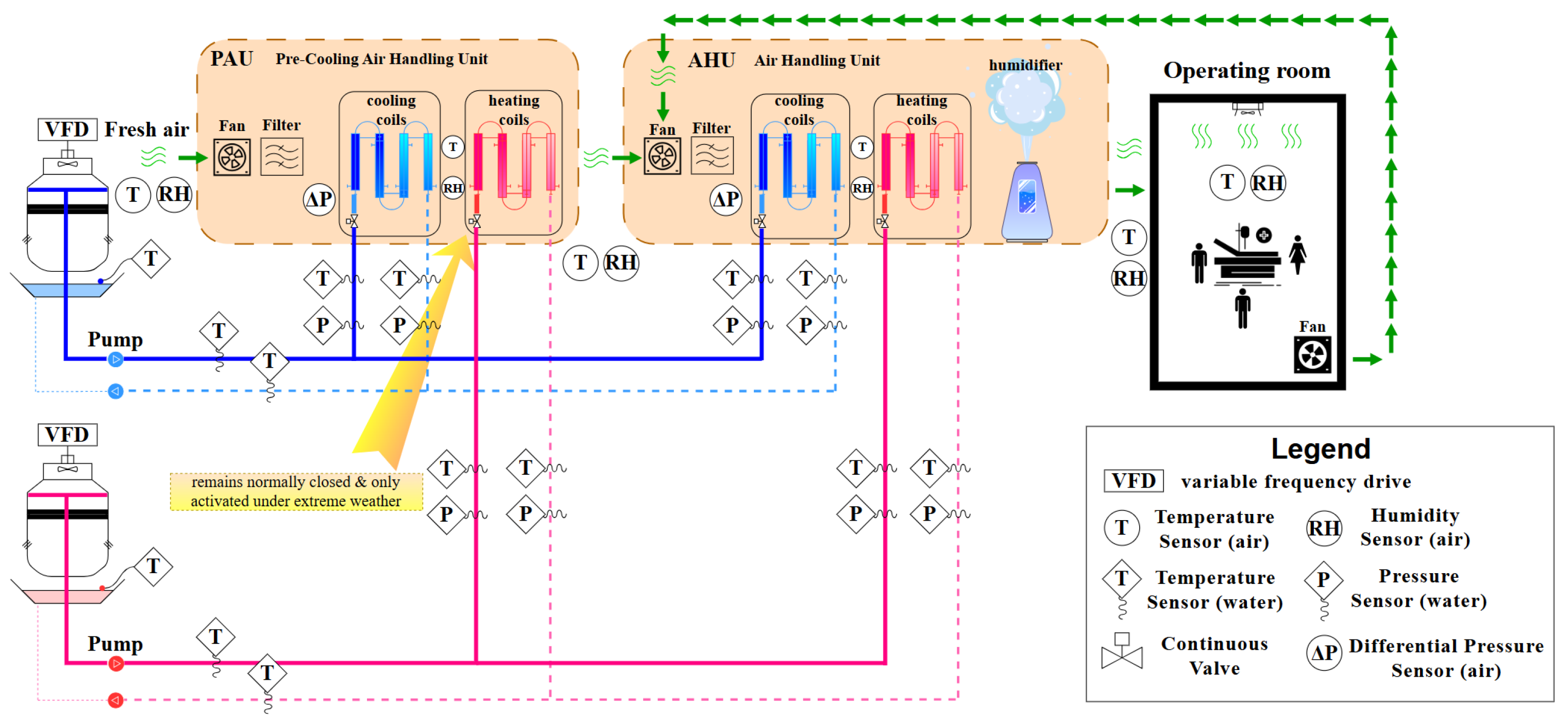
2.1. The HVAC System

To meet the air cleanliness requirements of the clean operating room, the HVAC system consists of an outdoor pre-cooling air handling unit (PAU) and an air handling unit (AHU), as shown in Figure 2. The air circulation process is as follows: outdoor fresh air is preconditioned by the AHU, mixed with return air, and then processed by the air handling unit (AHU) before being supplied to the indoor space. The water system is supported by two variable frequency heat pumps providing chilled and heated water. The heat pump supplies chilled and hot water, which flows through coils to exchange heat with the air. After heat exchange, the water returns to the heat pump to be heated or cooled, completing the circulation process. The system is equipped with sensors to facilitate modeling and system identification.

The structures of the pre-cooling air handling unit (PAU) and the air handling unit are similar, including components such as filters, variable frequency fans, cooling coils, heating coils, and humidifiers. In addition to providing temperature control during the winter, the heating coils also serve as reheating devices during the summer. The four-pipe system, consisting of the pre-cooling air handling unit (PAU) and air handling unit (AHU), offers greater flexibility in controlling the indoor thermal environment.

The PAU is exclusively designed for outdoor air processing. It extracts fresh air directly from the outdoor environment and performs preconditioning operations including dehumidification and dust filtration. The primary function of the PAU is to supply pretreated and dehumidified fresh air, without undertaking thermal and moisture load regulation in the operating theater zone, thereby serving an auxiliary control role. In contrast, the air handling unit (AHU) primarily processes mixed airflow comprising PAU exhaust air and operating room return air. As the core load-bearing component, the AHU assumes responsibility for thermal–hygric load management within the surgical environment and executes direct closed-loop control over temperature and humidity parameters in the operating theater. The cooling coils in both units achieve the separation of cooling and dehumidification, effectively reducing energy consumption caused by additional reheating devices. Additionally, it is important to note that the internal structure of the PAU, as depicted in Figure 2, also includes a heating coil. However, this coil is only utilized when the outdoor temperature drops below freezing to prevent the risk of pipe freezing or damage to the pipes. This study does not address control strategies under such extreme weather conditions.

In the HVAC system, sensors used for monitoring air conditions include integrated temperature and humidity sensors, as well as differential pressure sensors. The integrated temperature and humidity sensors are positioned at the air intake and exhaust outlets of both units. Additionally, integrated temperature and humidity sensors are installed inside the operating room. Furthermore, a set of integrated temperature and humidity sensors is installed outside the PAU air intake to measure outdoor environmental parameters. Differential pressure sensors are located before and after the fans and filters of both units. Temperature and pressure sensors are installed in the supply and return water pipelines to measure the temperature and pressure of the chilled water supply and return. The detailed specifications of the aforementioned sensors and valves are summarized in

Table 1. Specifications of sensors installed in the operating room.

Location	Sensor	Variables	Specifications	Range	Accuracy
Operating room	THPL	Temperature and RH	MN-ENV-THPL	−20 to 85 °C	±0.25 °C
				0 to 99.99%	±3%
HVAC	Combined temp. and RH	Temperature and RH	FG	−10 to 70 °C	±0.25 °C
				0 to 99.99%	±3%
	Pressure sensor	Differential pressure	HALO-FY-WG	0 to 1500 Pa	±0.5 Pa
	Pressure sensor	Water pressure	RL-132	0 to 500 kPa	±0.5 kPa
	Temperature sensor	Water temperature	RL-131	−10 to 60 °C	±0.5 °C
Outdoor	Combined temp. and RH	Temperature and RH	MN-ENV-THPL	−20 to 85 °C	±0.25 °C
				0 to 99.99%	±3%

, as shown below.

The thermal gain in the room originates from occupant activities, heat exchange with the building walls, and the thermal energy from the HVAC system. The pre-cooling air handling unit (PAU) and air handling unit (AHU) exchange heat through cooling and heating coils. A mechanistic modeling approach is used to model the thermal dynamics of the AHU and the room [36].

The dynamic modeling approach for the cooling and heating coils of both the pre-cooling air handling unit (PAU) and air handling unit (AHU) is the same. The dynamic modeling is based on the following assumptions:

(1) The effects of temperature and pressure on the thermophysical properties of air and water are neglected.

(2) The temperatures of the chilled (or heated) water inside the coils, as well as the average temperature and humidity of the air passing through the coils, are approximated as the arithmetic mean of the air (or water) inlet and outlet parameters.

(3) During the dehumidification process, the condensate on the cooling coils is assumed to form a uniform water film, with the additional thermal resistance from the condensate film accounted for in the convective heat transfer resistance on the air side [37].

(4) Due to the large number of coil rows, the heat exchange performance is relatively high, and the bypass air ratio is low. Therefore, in this study, the influence of the bypass factor on heat transfer calculations is neglected, as the associated error is within an acceptable range.

Based on the aforementioned assumptions, the thermal balance equations for the cooling and heating coils are established using the principles of mass and energy conservation [37]:

$${\displaystyle \frac{1}{2}}{\rho }_w{c}_w{A}_{w}l{\displaystyle \frac{d(t_{w,L}+t_{w,E})}{d\tau }}=G_{w,E}{c}_w(t_{w,E}-t_{w,L})+a_{gw}{A}_i(t_g-{\displaystyle \frac{t_{w,L}+t_{w,E}}{2}})$$

(1)

In Equation (1), ρ_w represents the density of water (kg/m³); C_w denotes the specific heat capacity of water (J/(kg·°C)); A_w is the heat exchange area between the coil and the air (m²); l is the length of the coil (m); t_w,L is the water outlet temperature of the coil (°C); t_w,E is the water inlet temperature of the coil (°C); τ is the time (s); G_w,E is the mass flow rate of water entering the coil (kg/s); a_gw is the heat transfer coefficient between the water and the external surface of the finned heat exchanger (W/(m²·°C)); A_i is the internal surface area of the heat exchanger tube (m²); and t_g is the wall temperature of the surface-type heat exchanger tube (°C).

The energy balance equation for the air flowing through the coil is as follows [37]:

$${\displaystyle \frac{1}{2}}{\epsilon }_a{\rho }_{a}b{A}_a{\displaystyle \frac{d(h_{a,L}+h_{a,E})}{d\tau }}=G_{a,E}(h_{a,E}-h_{a,L})+a_{ga}{A}_o(t_m-{\displaystyle \frac{t_{a,L}+t_{a,E}}{2}})+q_r{A}_o{\lambda }_m(W_{gb}-{\displaystyle \frac{W_{a,E}+W_{a,L}}{2}})$$

(2)

In Equation (2), b represents the duct width (m); h_a,L denotes the air enthalpy at the outlet side (J/kg); h_a,E represents the air enthalpy at the inlet side (J/kg); q_r is the latent heat of condensation (J/kg); G_a,E is the mass flow rate of air entering the duct (kg/s); A_o is the external surface area of the heat exchanger tube (m²); W_gb refers to the moisture content of the air near the surface of the heat exchanger’s finned surface under wet operating conditions (kg/kg); a_ga is the heat transfer coefficient between the air and the external surface of the finned heat exchanger (W/(m²·°C)); W_a,E is the moisture content of air at the inlet side; and W_a,L is the moisture content of air at the outlet side.

The humidity balance equation for the air flowing through the coil s as follows [37]:

$${\displaystyle \frac{1}{2}}{\epsilon }_a{\rho }_{a}b{A}_a{\displaystyle \frac{d(W_{a,L}+W_{a,E})}{d\tau }}=G_{a,E}(W_{a,E}-W_{a,L})+A_o{\lambda }_m(W_{gb}-{\displaystyle \frac{W_{a,E}+W_{a,L}}{2}})$$

(3)

In Equation (3), ε_a represents the air-side air ratio of the coil; λ_m denotes the convective mass transfer coefficient of the coil heat exchanger (kg/(m²·s)).

When modeling the operating room, the following assumptions are made:

(1) The air inside the operating room is assumed to be fully mixed and is described by a single state.

(2) Radiative heat transfer between the room’s walls and objects is negligible. In dynamic response simulations, the convective heat transfer coefficients between the walls or between heat sources and the surrounding air are considered constant [38].

Based on these assumptions and according to the laws of mass and energy conservation, energy and mass balance equations for the air and walls in the operating room can be established.

The energy balance equation for the room temperature is as follows [38]:

$$T_{\tan }{\displaystyle \frac{d\Delta t_{a,n}}{d\tau }}=X_{\tan ,1}\Delta t_{a,s}+X_{\tan ,2}\Delta t_{a,n}+X_{\tan ,6}\Delta G_{a,s}+{\displaystyle \sum _{i=1}^k{X}_{\tan ,7}^{(i)}}\Delta A_{rq,n}^{(i)}$$

(4)

The coefficients in the equation are expanded as follows:

$$T_{\tan }=c_a{\rho }_a{V}_{a,n}$$

$$X_{\tan ,1}=(c_a{G}_{a,s}+a_{as-an}{A}_{as-an})$$

$$X_{\tan ,2}=(-c_a{G}_{a,s}+0.934c_a{C}_{res}{M}_{body}{A}_{rq,n}^1+a_{riw,n}{A}_{riw,n}+a_{rew,n}{A}_{rew,n}+a_{as-an}{A}_{as-an}+a_{an-ar}{A}_{an-ar}+{\displaystyle \sum _{i=1}^k{a}_{rq,n}}{A}_{rq,n}^i)$$

$$X_{\tan ,6}=c_a(t_{a,s}-t_{a,n})$$

$$X_{\tan ,7}^i=a_{rq,n}(t_{rq,n}^i-t_{a,n}^i)$$

In the equation, c_a represents the specific heat capacity of the air in the operating room; ρ_a denotes the air density in the operating room (kg/m³); V_a,n is the volume of the operating room (m³); G_a,s is the increment of the air supply flow rate to the operating room; a_as-an is the convective heat transfer coefficient of the air (W/(m²·°C)); A_as-an is the supply air outlet area (m²); a_an-ar is the convective heat transfer coefficient of the air at the exhaust outlet (W/(m²·°C)); A_an-ar is the exhaust air outlet area (m²); C_res is a proportional constant, equal to 1.43 × 10⁻⁶ kg/J; M_body and H_body are the body weight and height of the individuals in the room; $A_{rq,n}^{\left(i\right)}$ is the body surface area of the individuals (m²); a_rq,n is the heat transfer coefficient of the human body (W/(m²·°C)); a_riw,n is the convective heat transfer coefficient of the operating room’s internal walls (W/(m²·°C)); A_riw,n is the area of the internal walls of the operating room (m²); a_rew,n is the convective heat transfer coefficient of the operating room’s external walls (W/(m²·°C)); and A_rew,n is the area of the external walls of the operating room (m²).

The humidity energy balance equation for the room is as follows [38]:

$$T_{wan}{\displaystyle \frac{d\Delta W_{a,n}}{d\tau }}=X_{wan,1}\Delta W_{a,s}+X_{wan,2}\Delta W_{a,n}+X_{wan,3}\Delta G_{a,s}+{\displaystyle \sum _{i=1}^k{X}_{wan,4}^{(i)}}\Delta A_{rq,n}^{(i)}$$

(5)

The coefficients in the equation are expanded as follows:

$$T_{wan}={\rho }_a{V}_{a,n}$$

$$X_{wan,1}=G_{a,s}$$

$$X_{wan,2}=-0.8C_{res}{M}_{body}{A}_{rq,n}^1-G_{a,s}$$

$$X_{wan,3}=W_{a,s}-W_{a,n}$$

$$X_{wan,4}=C_{res}{M}_{body}(0.02933-0.8W_{a,n})$$

In the equation, W_a,s represents the supply air humidity; W_a,n denotes the humidity in the operating room; t_a,s is the supply air temperature from the unit (°C); and t_a,n is the temperature in the operating room (°C).

Specific parameter values are provided in

Table 2. Summary of the operating room structural parameters and internal air conditions parameters.

Parameter	Value	Parameter	Value
Operating room volume V, m3	114	Air supply outlet area Aas-an, m2	20
Specific heat capacity of room wall criw,n, J/(kg·°C)	1250	Air convective heat transfer coefficient aas-an, W/(m2·°C)	5
Density of room wall ρriw,n, kg/m3	1800	Pulmonary ventilation rate constant Cres, kg/J	1.43 × 10−6
Specific heat capacity of air ca, J/(kg·°C)	1005	Air density ρa, kg/m3	1.18

and

Table 3. Summary of the basic structural parameters of the evaporator coil.

Parameter	Value	Parameter	Value
Coil Length l, m	15	Windward Area Aa, m2	1.75
Inner Radius of the Evaporator Coil Finned Tube ri, m	0.004	Finned Tube Pitch of the Evaporator Coil agw, W/(m2·°C)	0.0024
Inner Surface Area of the Evaporator Coil Finned Tube Ai, m2	0.5287	Thickness of the Fins on the Evaporator Coil Finned Tube δc, m	0.0002
Outer Surface Area of the Evaporator Coil Finned Tube Ao, m2	8.8065	Mass of the shell wall of a surface-type heat exchanger Mg, kg	7.52
Dimension along the Air Flow Direction b, m	0.66	Specific Heat Capacity of the Evaporator Coil Heat Exchanger Material Cg, J/(kg·°C)	475

.

In Equations (1)–(5), Δt_a,s represents the temperature increment of the incoming air to the operating room, Δt_a,n denotes the temperature increment within the operating room, and ΔG_a,s indicates the flow rate increment of the incoming air to the operating room.

The system of Equations (1)–(5) is linearized by expressing the fundamental variables as the sum of their steady-state initial values and small increments. By combining the model of the air handling unit (AHU) with the operating room model, the above equations can be written in the state-space form of the surface heat exchanger using matrix representation:

$$\begin{array}{l}\dot{X}=A\cdot X+B\cdot u+W\cdot d\\ y=C\cdot X+D\cdot u\end{array}$$

In this model, X, u, and y represent the state, input, and output vectors, respectively. A, B, C, W, and D are the state matrix, input matrix, output matrix, disturbance matrix, and feedthrough matrix, respectively. The state and input descriptions of the state-space model are shown in

Table 4. Inputs and states for state-space model.

States	Description	Inputs	Description
LΔtw,L	The cooling coil outlet water temperature	LΔGw,E	The cooling coil outlet water flow rate
LΔta,L	The cooling coil outlet air temperature	HΔGw,E	The heating coil outlet water flow rate
LΔWa,L	The cooling coil outlet air humidity	ΔGa,E	The coil outlet air flow rate
HΔtw,L	The heating coil outlet water temperature	ΔGa,s	The operating room intake air flow rate
HΔta,L	The heating coil outlet air temperature
HΔWa,L	The heating coil outlet air humidity
Δta,n	The operating room temperature
ΔWa,n	The operating room humidity

. The output and disturbance descriptions of the state-space model are provided in

Table 5. Outputs and disturbances for state-space model.

Disturbances	Description	Outputs	Description
LΔtw,E	Cooling coil inlet chilled water temperature	Δta,n	The operating room temperature
LΔta,E	Cooling coil inlet air temperature	ΔWa,n	The operating room humidity
LΔWa,E	Cooling coil inlet air humidity
HΔtw,E	Heating coil inlet air temperature

. In the table, Δ represents the increment.

2.2. MPC Controllers

An MPC controller was developed to regulate the chilled and hot water flow rates of the air handling unit’s (AHU) coils. The pre-cooling air handling unit (PAU) regulates the pre-treatment of the fresh air, eliminating potential and partial sensible loads, while the AHU handles the remaining sensible load [39].

The two MPC controllers have the same overall structure, as shown in Figure 3, consisting of an optimization solver, a state-space model, constraints, and a cost function.

The MPC optimizes the cooling power provided by the chilled water in the cooling coil of the air handling unit (AHU) based on the objective function in Equation (6), while minimizing control actions within the prediction horizon.

$$J=Minimize({\displaystyle \sum _{k=0}^N{‖T_{t+k|t}^{obj}-T_{t+k|t}‖}_{Q_T}^2+{\displaystyle \sum _{k=0}^N{‖W_{t+k|t}^{obj}-W_{t+k|t}‖}_{Q_H}^2}+{‖u_t‖}_R^2}+{\displaystyle \sum _{k=0}^N{W}_{\epsilon }{({\epsilon }_{t+k|t})}^2})$$

(6)

In the equation, $T_{t+k|t}^{obj}$ represents the temperature control setpoint for the operating room, $W_{t+k|t}^{obj}$ represents the humidity control setpoint for the operating room, u_t represents control input, W_ε(ε_t+k|t) denotes the penalty term for constraint violations, Q_T and Q_H represent the weight matrices for temperature and humidity, respectively, which determine the significance of errors in the optimization objective, and R is the cost matrix for control inputs, designed to prevent instability caused by excessive control signals.

The chilled and hot water are directly supplied by two outdoor heat pump units, with water temperature regulation automatically managed by the built-in control program of the system. The MPC does not involve the adjustment of the heat pump’s outlet water temperature. Furthermore, the heat pump is assumed to maintain relatively stable water temperature control (±5 °C). In the control model, the impact of the outlet water temperature is categorized as a disturbance variable and represented in matrix form.

Due to the specific environmental requirements of the operating room, which necessitate maintaining a positive pressure environment and ensuring an air exchange rate of 20 times per hour, this study adopts a constant air volume (CAV) control strategy, meaning that the supply airflow rate remains unchanged. In the input matrix, although the airflow increment is still included as a control input variable, its weighting coefficient is set to zero to reflect its constant state.

Due to the use of cooling coils for dehumidification in the system, the MPC faces a conflict between controlling the humidity and reducing the temperature, as lowering the temperature conflicts with the objective of maintaining a constant temperature.

However, thanks to the presence of the pre-cooling air handling unit (PAU), its cooling coils effectively control the fresh air humidity load in the clean operating room, allowing for the separation of temperature and humidity control objectives. Specifically, the PAU is responsible for cooling and dehumidification, while the air handling unit (AHU) is tasked only with air reheating and regulating the thermal and humidity load in the clean operating room. However, the setpoint for the outlet air temperature of the PAU is influenced not only by outdoor meteorological conditions but also by the indoor temperature and humidity conditions and control targets. Typically, previous decisions are made based on human experience combined with on-site conditions; however, this requires extensive experience accumulation and has a high learning cost. Therefore, this complex multivariable decision-making process is optimized and managed by a large language model to ensure precise and efficient control performance.

2.3. The MPC Framework Integrated with the Large Language Model (LLM)

Building upon the MPC-based lower-level controller, a control system was developed with LLM as the high-level decision-making core, as illustrated in Figure 4a.

The system adopts a hierarchical control architecture, wherein the lower-level controller utilizes Model Predictive Control (MPC) for precise regulation, while higher-level decision making relies on a Large Language Model (LLM) to provide intelligent optimization strategies. The core objective of this control architecture is to optimize the operation of the HVAC (Heating, Ventilation, and Air Conditioning) system through the advanced reasoning capabilities of the LLM, without altering the underlying MPC structure, in order to achieve precise control of temperature and humidity as well as energy consumption optimization.

The high-level decision-making layer is based on LLM-driven control optimization, where the LLM is responsible for conducting a high-level analysis of the HVAC system’s operational state and generating interpretable control strategies to guide the adjustment of MPC parameters. Specifically, the control logic of the LLM includes the following key steps:

• Environmental Information Parsing: The LLM extracts current operating conditions from sensor data, including outdoor and indoor temperature and humidity, supply air temperature, and the operational status of the pre-cooling air handling unit.
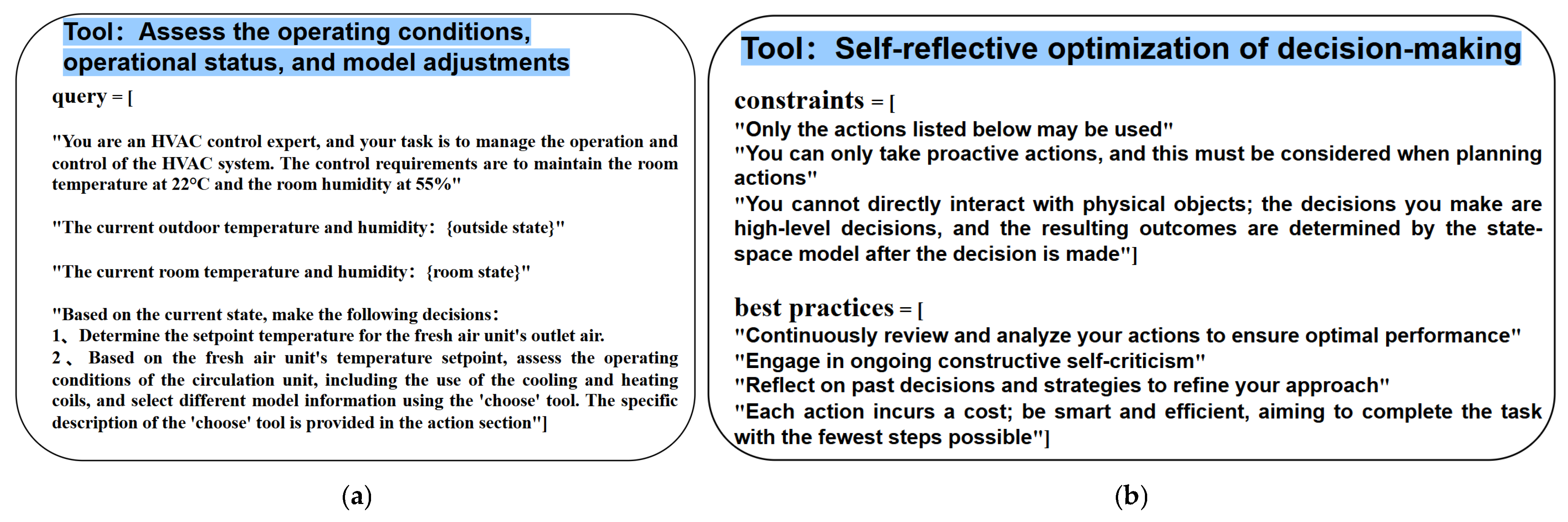
• State Evaluation and Pattern Recognition: Based on the input environmental data and utilizing the HVAC domain knowledge base and historical interaction data, the LLM identifies the current operational mode (e.g., cooling and dehumidifying, heating and humidifying, etc.).
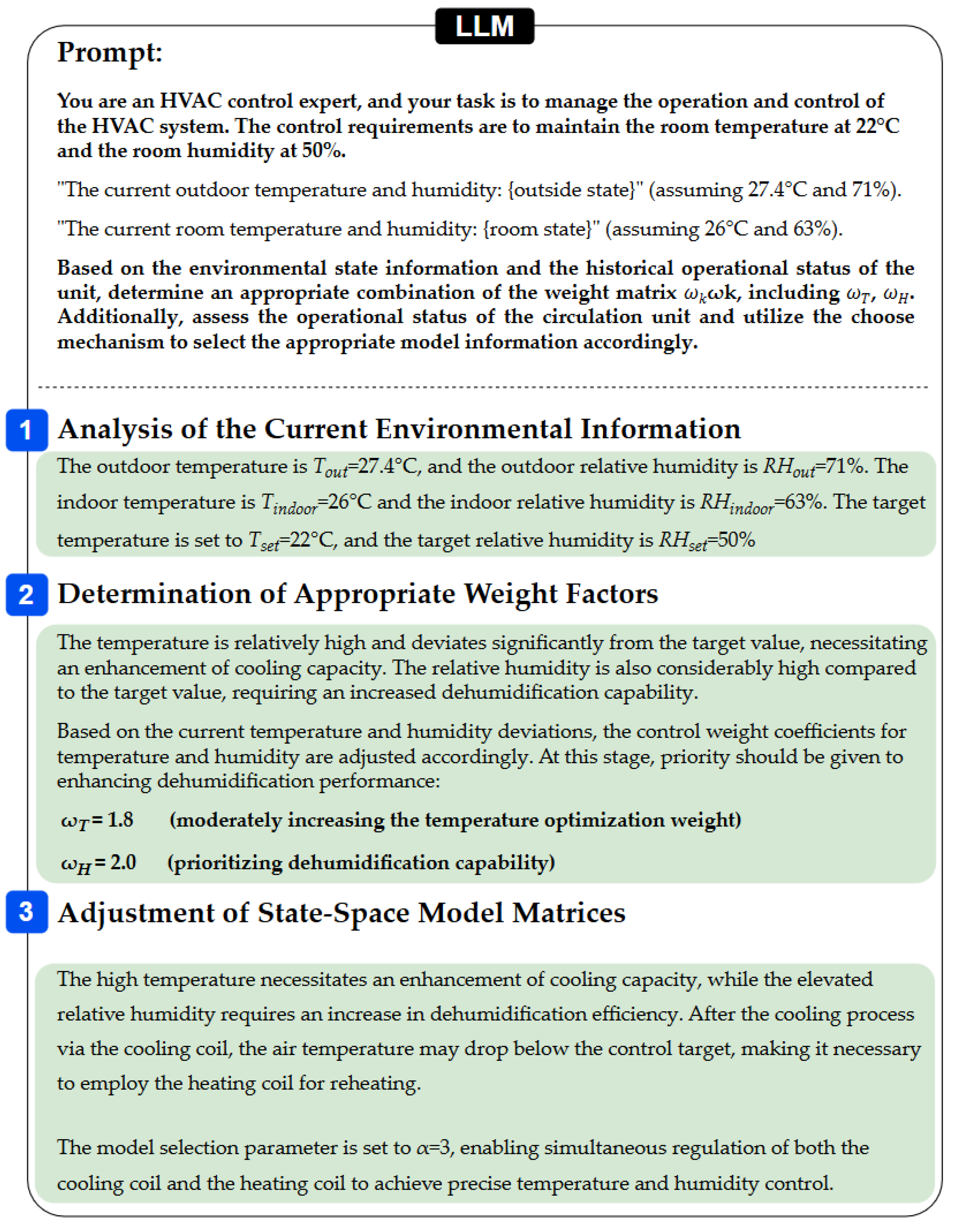
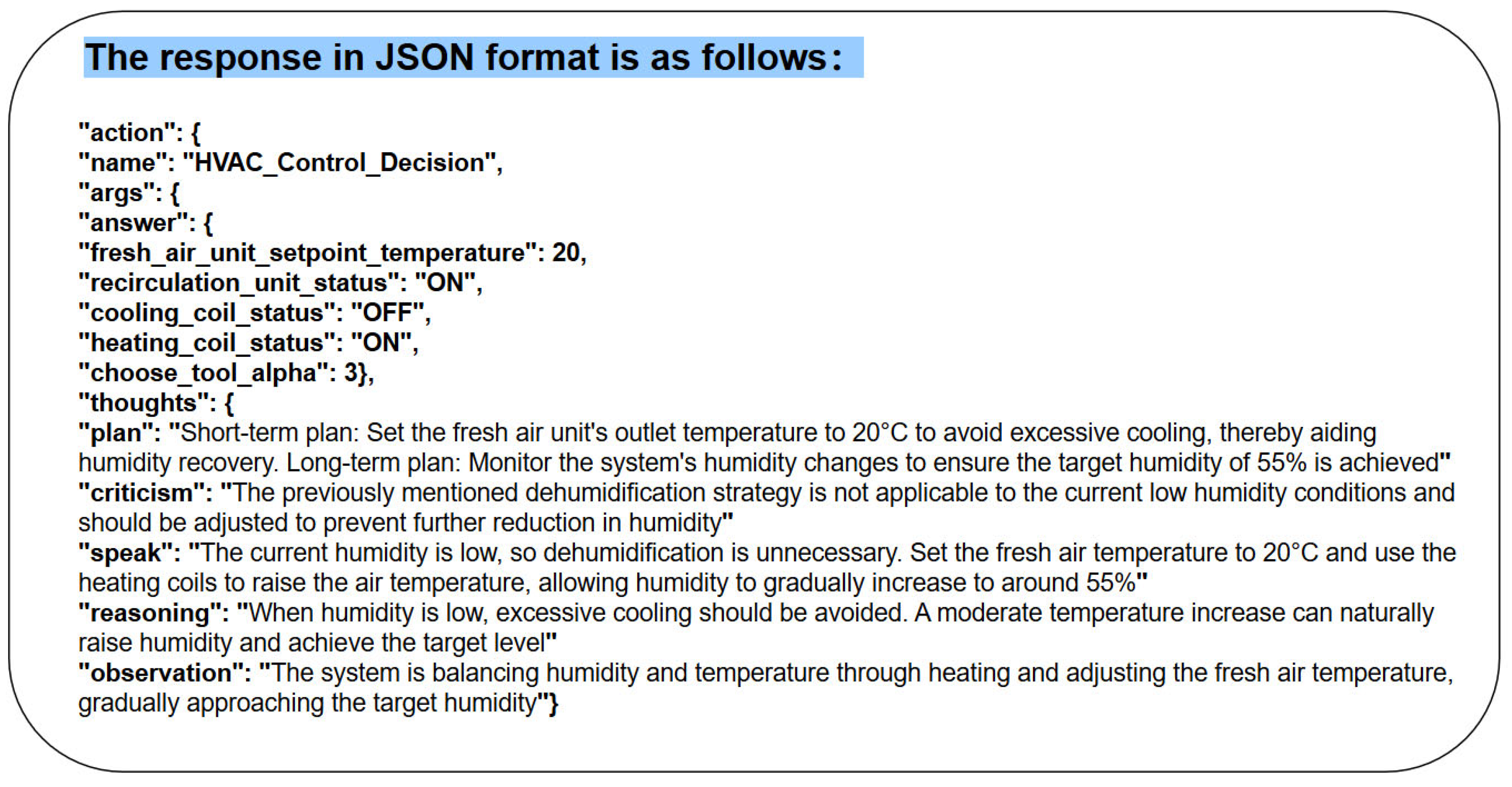
• Control Strategy Generation: Based on the state evaluation, the LLM generates targeted optimization strategies through chain-of-thought reasoning. This primarily involves adjusting the weights of the MPC objective function to accommodate the control demands of different operating conditions (e.g., in high-humidity situations, even if the temperature has reached the control target, the system will still prioritize using the AHU’s cooling coil for humidity control, while guiding the PAU unit to reduce the supply air temperature to enhance dehumidification).
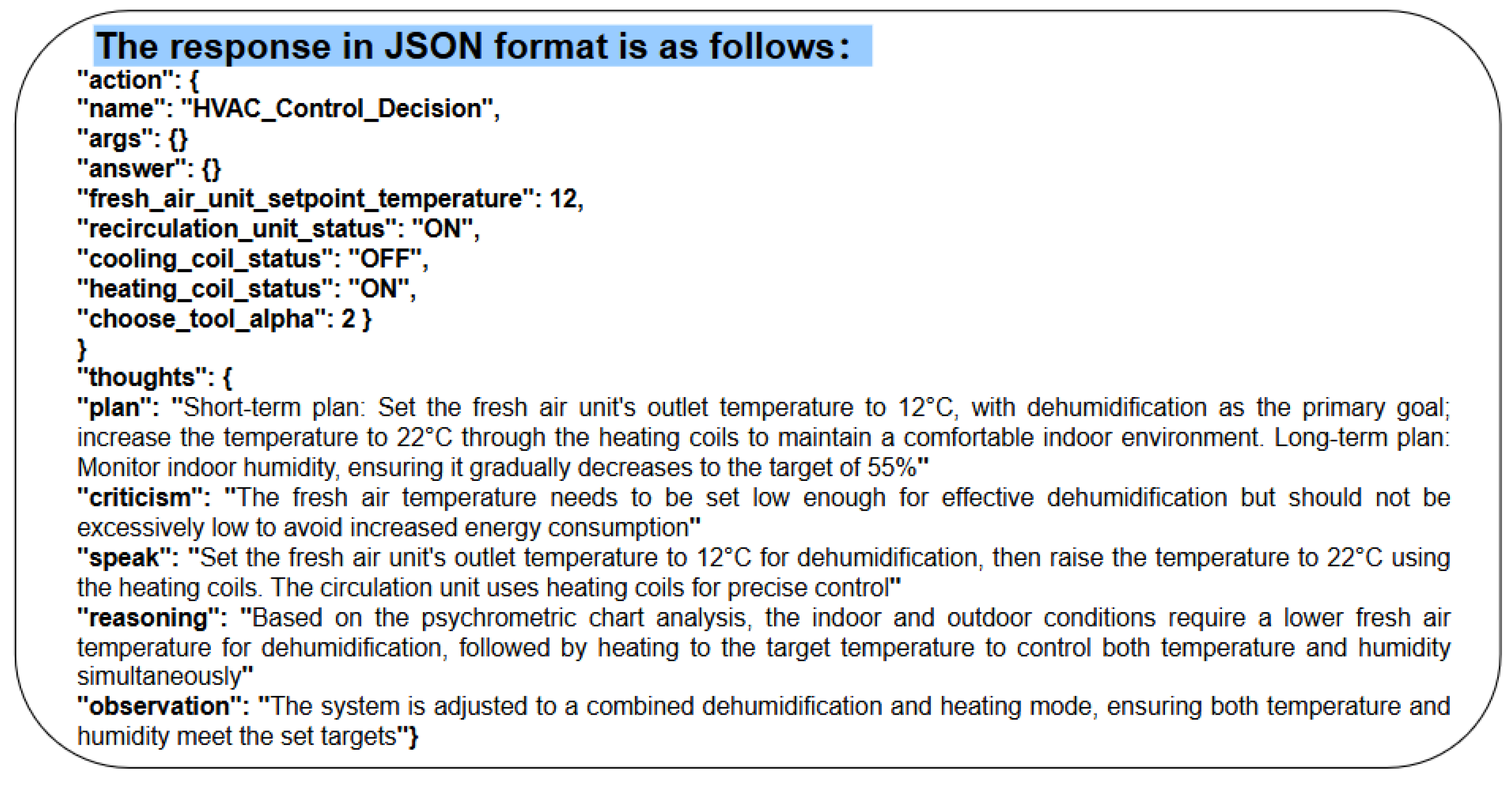
• Decision Conversion and Execution: The textual decisions generated by the LLM are parsed into numerical control instructions through function analysis and transmitted to the MPC for execution.

Figure 4b provides an example in hot and humid conditions, where the LLM needs to make specific high-level decisions. The LLM initiates a dialogue based on the provided prompts, continuously collects information from the environment, performs reasoning, and makes judgments. As shown in the center of Figure 4a, from left to right, the LLM sequentially: (1) evaluates the current state information, identifies the operating conditions of the pre-cooling air handling unit (PAU), and determines the control actions potentially needed for the air handling unit (AHU); (2) provides specific action guidance. The system then converts these two high-level text decisions into executable function representations.

MPC utilizes a mathematical model of the controlled system to predict its future states and formulates current control actions based on these predictions. During the MPC process, predefined weight matrices are typically used. However, these fixed weights cannot dynamically adapt to varying environmental conditions. This is particularly problematic in high-precision scenarios such as operating rooms, where traditional MPC may suffer from high computational complexity, insufficient adaptability, and difficulty in accurately balancing temperature and humidity control. Therefore, it is necessary to introduce a higher-level decision-making mechanism to optimize the MPC strategy, thereby enhancing its adaptability and performance across different operating conditions.

Within the framework of the Markov Decision Process (MDP), the HVAC control problem is first reformulated as shown in Equation (7):

$$M=(S,A,P,R,\gamma )$$

(7)

In Equation (7), S represents the state space, encompassing environmental variables such as temperature and humidity, A denotes the action space, including HVAC control inputs such as cold water and hot water valves, P(s’|s,a) represents the state transition probability, describing the physical dynamics of the HVAC system from state S_t to S_t+1, R(s,a) is the reward function, reflecting the optimization direction of the control objectives, and γ is the discount factor, controlling the trade-off between short-term and long-term optimization.

At this point, the MPC objective function is extended into the MDP framework, and the MPC objective function can be restructured as Equation (8):

$$J={\displaystyle \sum _{t=0}^T{\gamma }^{t}R(s_t,a_t)}$$

(8)

In the equation, the definition of the reward function R(s,a) is as follows:

$$R(s,a)={\displaystyle \sum _{k=0}^N{\omega }_k\cdot n_k(r_k(s,a,{\phi }_k))}$$

In the equation, ω_k represents the dynamically adjusted weight matrix, which primarily includes ω_T and ω_H, corresponding to the temperature and humidity control weights, respectively, and is controlled by the LLM; n_k(⋅) denotes the error norm (l₂ norm); r_k(s,a,φk) is the residual term, used to quantify the control error. By extending the MPC objective function into the MDP framework, the weight coefficients ω_k and the residual term r_k are dynamically optimized by the LLM, enabling the HVAC control to adaptively adjust under varying operational conditions, rather than solely relying on preset fixed weights.

The residual term r_k represents the error term in HVAC control, which can be specifically defined as Equation (9).

$$r_T=T_{set}-T_{actual}, r_H=H_{set}-H_{actual}$$

(9)

In the LLM-assisted MPC control, the l₂ norm is used to calculate the optimization objective, as shown in Equation (10):

$$C_T={\omega }_T\cdot {(r_T)}^2, C_H={\omega }_H\cdot {(r_H)}^2$$

(10)

In the equation, ω_T and ω_H represent the dynamically adjusted weighting factors, controlled by the LLM, which are dynamically adjusted based on environmental conditions and control objectives, and r_T and r_H are the values measured in real-time by sensors and fed back into the control system.

This study employs the Large Language Model (LLM) for dynamic adjustment, where the LLM analyzes historical data and environmental variables to dynamically generate combinations of ω_k, thereby enhancing the adaptive capability of the HVAC control system. The LLM acquires HVAC control knowledge through large-scale training data and generates high-level weighting adjustment strategies during the inference process.

For example, under operating conditions where cooling and dehumidification are required in the summer, the relationship between ω_T and ω_H is given by Equation (11), indicating that the priority of dehumidification or humidity control exceeds that of temperature control.

$${\omega }_H^{summer}>{\omega }_T^{summer}$$

(11)

At this point, the objective function of the MPC is optimized by the LLM, as shown in Equation (12).

$$J={\displaystyle \sum _{t=0}^T{\gamma }^t}{\displaystyle \sum _{k=0}^N{\omega }_k^{*}\cdot n_k(r_k(s,a,{\phi }_k))}, {\omega }_k^{*}=LLM(s_t,s_{t-1},\dots ,s_{t-k})$$

(12)

In the equation, ${\omega }_k^{*}$ represents the weight matrix dynamically adjusted by the LLM, which is inferred by the LLM based on the current environmental state and control objectives, as well as other environmental state information S_t, in order to derive the optimal weight parameters.

Moreover, the LLM is required not only to provide the weight coefficients ω_k, by considering the current environmental state and control objectives but also to evaluate and adjust the state-space model matrix used by the MPC. At this point, the discrete dynamic model of the system state is represented as Equation (13):

$$X_{t+1}=A_{\alpha }{X}_t+B{u}_t+W{d}_t$$

(13)

The model selection parameter α is used to dynamically adjust the system state transition matrix A, and it is dynamically selected by the LLM to optimize the state-space representation used during the MPC computation process. The value of α takes different values, which determines the control mode of the MPC. Specifically, when α = 1, only the cooling coil is used for control; when α = 2, only the heating coil is used for control; and when α = 3, both the cooling and heating coils are required. By assigning zero to the matrix elements corresponding to different coils in the state matrix A_α, the switching between different coil control modes is realized. Based on this, the LLM can dynamically adjust the value of α under different operating conditions, allowing the MPC to select the specific coil for control during the optimization process, thereby reducing computational complexity and improving control efficiency.

Figure 5 illustrates the detailed process through which the LLM provides high-level decision making.

This adjustment, which favors the use of a specific coil for control, facilitates the effective transition from high-level decisions to lower-level control logic [40]. This process ensures the coordination between the pre-cooling air handling unit (PAU) and the air handling unit (AHU), thereby optimizing the overall system’s control performance. These elements, as instructions for the MPC lower-level controller, guide the MPC to optimize the objective function and determine the specific valve opening actions.

Two tools are designed, as shown in Figure 6: the “condition assessment, operating state, and model adjustment” tool and the “self-reflection optimization decision” tool. Each tool plays a specific role within the structured thinking chain and assists the LLM in reasoning and decision making through a series of constraints and best practices [41].

The query section of the LLM defines the current environmental state, such as indoor and outdoor temperature and humidity information, to infer the operational status of the equipment, including the operation of the air handling unit (AHU) and the room humidity controller. Based on this, the LLM performs multi-step reasoning, using the “choose” tool to explain its decision-making process and ensure real-time acquisition of state inputs during adjustments. The LLM utilizes real-time data to assess the operating conditions and adaptively adjust the control strategy, thereby improving the accuracy of the system model and the control performance. The “choose” tool further aids the LLM in structurally transmitting the reasoning results to subsequent steps, forming a feedback loop.

The self-reflection optimization decision tool of the LLM consists of two components: constraints and best practices. The constraints section imposes limitations on the decision-making conditions, such as restricting selections to a specified list of actions, ensuring that the LLM’s decisions within a complex system remain aligned with the primary objectives and maintain the integrity of the optimization process. The best practices define optimal strategies, streamlining the analytical process by reducing steps and enhancing efficiency. With these guidelines, the LLM can review its actions after making decisions, identify optimization opportunities, and simplify the operational process. Given the infrequency of operational condition changes in HVAC systems, frequent control decisions are unnecessary. Therefore, the reflection tool improves the efficiency and accuracy of LLM’s decisions, allowing it to gradually adapt to long-term operational requirements, thereby enhancing system stability, reducing repetitive decisions, and increasing overall efficiency.

3. Case Study

3.1. Simulation Arrangement

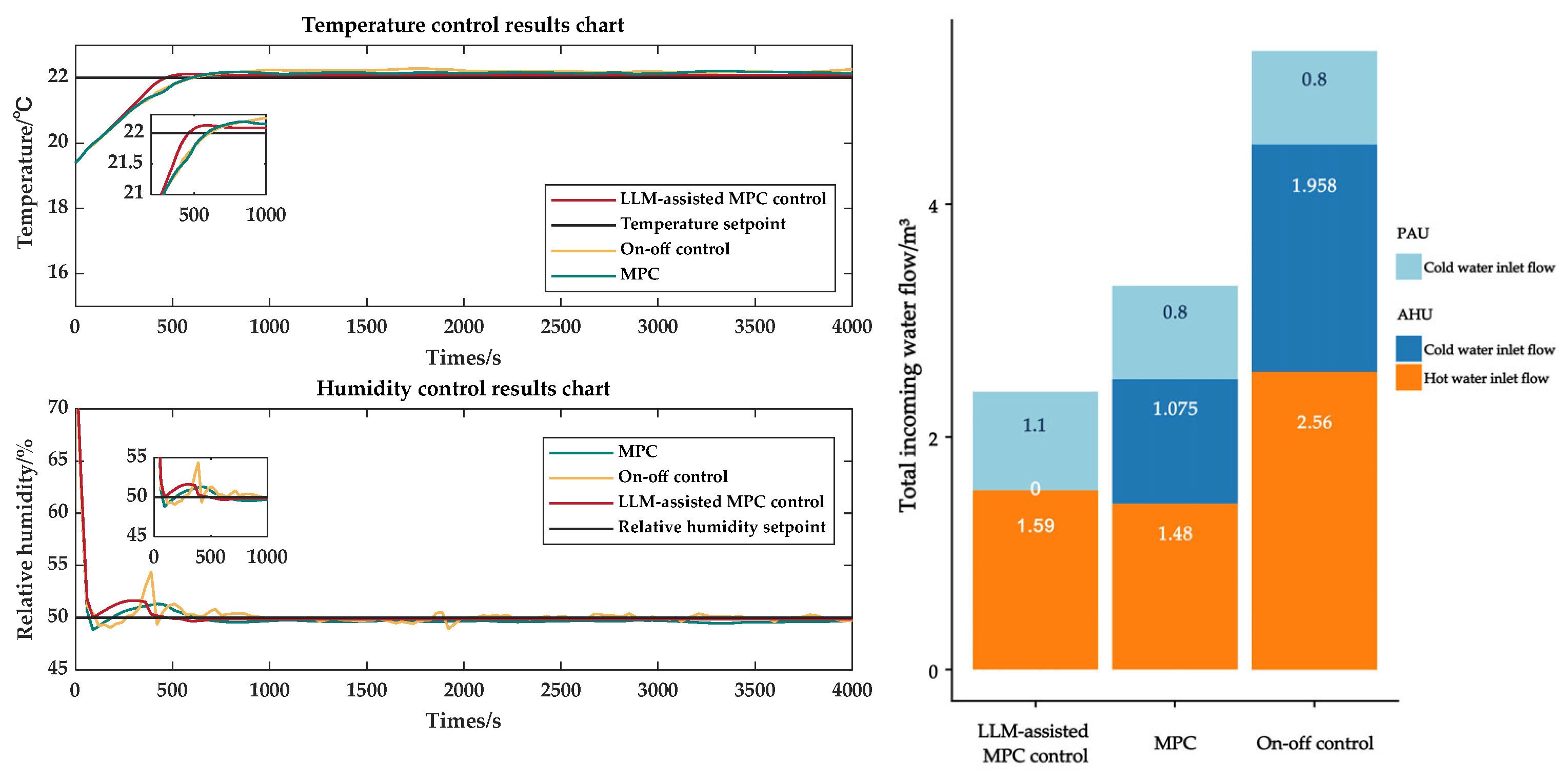
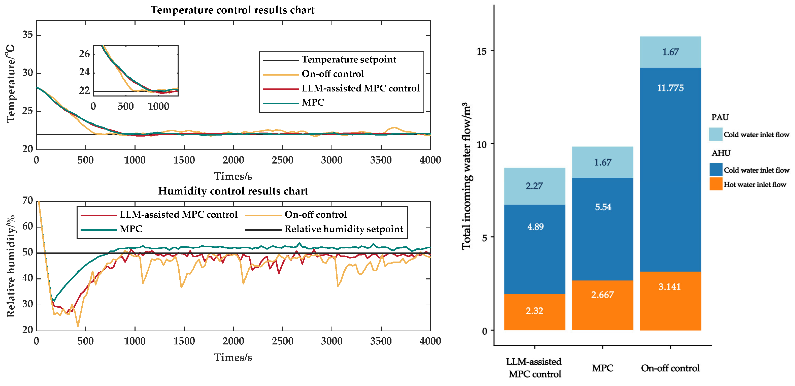
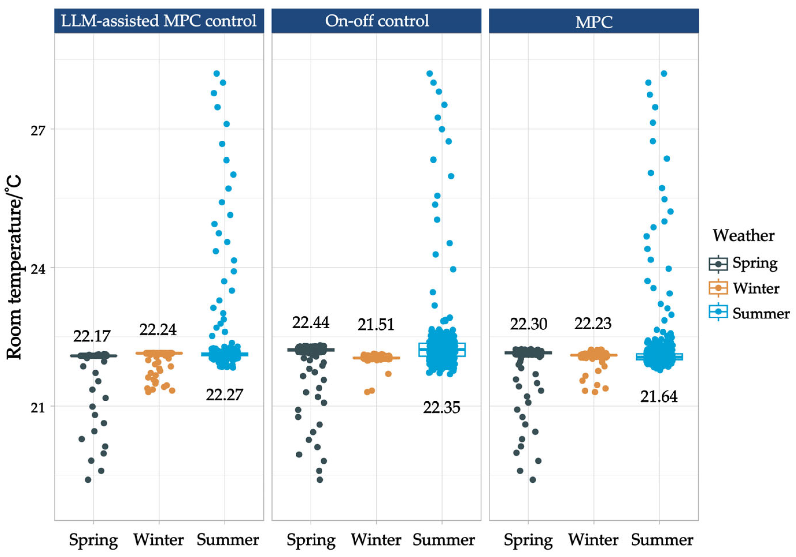
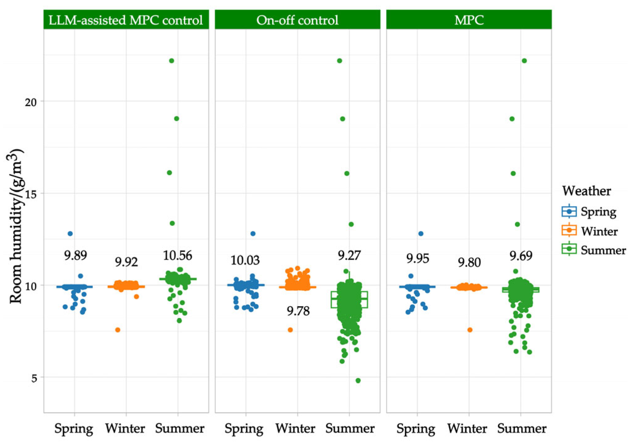
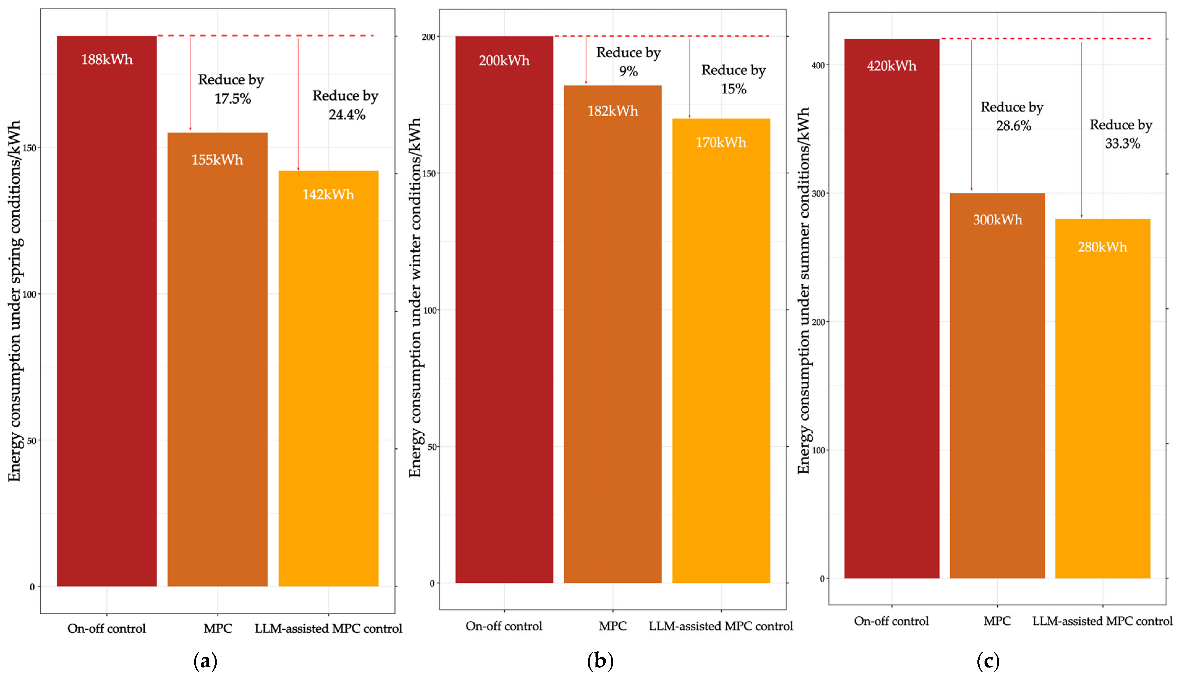
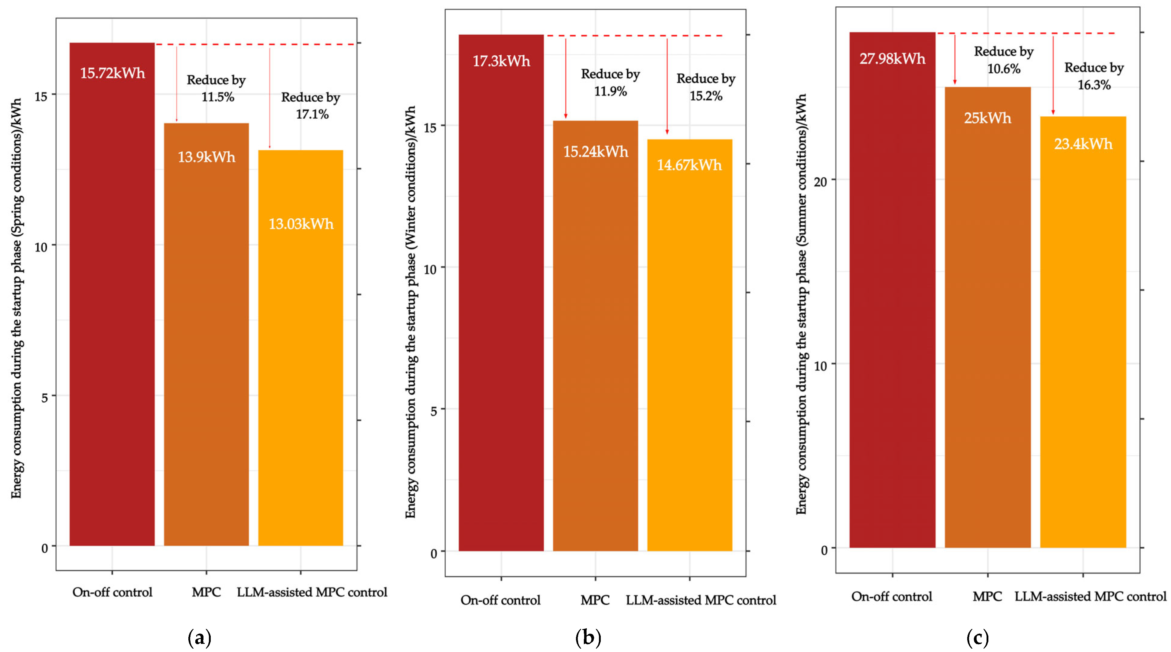
A 4 h simulation of the HVAC system was conducted, with the air control targets for the operating room set to a dry bulb temperature range of 22 °C to 24 °C and a relative humidity range of 40–60%, employing a constant air volume ventilation strategy. To evaluate the performance of the LLM-optimized Model Predictive Control (MPC) strategy, a comparison was made between the LLM-optimized MPC and the basic MPC strategies. The experimental environment simulated in this study is a hospital operating room, which is a highly sealed space located within the building. Heat exchange with the external environment primarily occurs through the ventilation system, and the impact of heat transfer through the walls is considered negligible. The simulation experiment is conducted within this enclosed space to replicate the air conditioning control performance under actual operating conditions.

In the comparative simulation experiments, the switch control strategy is used as the benchmark control method, with its operation logic based on fixed temperature and humidity setpoints. Specifically, when indoor temperature or humidity deviates from the set range, the system operates at maximum cooling/heating capacity until the setpoint range is restored. The specific setting of this strategy is as follows: when the indoor temperature exceeds the set value of 22 °C, the system uses the cooling coil to lower the temperature, and the cooling is turned off once the temperature falls below the set value.

To evaluate the LLM-optimized MPC strategy, a basic MPC was used as a control group for comparison under the same conditions. The MPC simultaneously controls both the cooling coil and heating coil of the AHU, with the model selection parameter fixed at 3, and the dynamically adjusted weight parameters, ω_T and ω_H, remaining consistent.

The pre-cooling handling air unit (PAU) operates with an independent control strategy, based on fixed setpoints to ensure the stability of the supply air temperature. In spring, the supply air temperature of the pre-cooling air handling unit (PAU) is fixed at 15 °C to meet basic dehumidification requirements. In winter, the pre-cooling air handling unit (PAU) remains in the off state, only operating minimally to satisfy the heat pump’s minimum load requirements. In summer, the supply air temperature of the pre-cooling air handling unit (PAU) is fixed at 20 °C, ensuring sufficient dehumidification while keeping the supply air temperature closer to the indoor control target. Neither the MPC nor the switch control adjusts the setpoints for the pre-cooling air handling unit (PAU), instead using fixed control strategies.

The sampling interval for all three control methods is 30 s, and the prediction horizon is 14,000 s, which are identical across the methods.

The simulation was conducted based on actual weather conditions, selecting three typical operating scenarios for control performance analysis: spring, winter, and summer.

The initial conditions for the spring scenario were set as follows: outdoor temperature 18.5 °C, outdoor humidity 78%, indoor temperature of the operating room 19.4 °C, and indoor humidity 76%. The cold water inlet temperature was 9.9 °C, and the hot water inlet temperature was 49.1 °C.

The control decisions made by the LLM under the spring conditions are shown in Figure 7. Figure 8 presents a comparison of the control results for different algorithms under spring conditions. In the figure, the red, green, and yellow curves represent the LLM-assisted MPC curve, the MPC curve, and the on–off control curve, respectively.

The simulated experimental results indicate that the LLM-assisted MPC stabilizes the temperature at 22 °C within approximately 800 s, maintaining minimal fluctuations, thus demonstrating superior control stability. In comparison, although the MPC takes an additional 100 s to reach stability, the temperature fluctuations are relatively small.

On the other hand, the on-off control method approaches the target temperature within the initial 600 s but struggles to maintain stability, exhibiting higher temperature fluctuation frequencies. The energy consumption analysis shows that the cold water valve usage under LLM-assisted MPC remains steady, with a higher cooling demand in the early stages, but the fluctuations decrease once temperature and humidity stabilize, resulting in the lowest energy consumption.

In contrast, the MPC exhibits frequent fluctuations in cold water valve usage, especially during the first 800 s, leading to higher energy consumption, while the on–off control method demonstrates large fluctuations in cold water valve usage, resulting in the highest energy consumption.

The simulated experimental initial conditions for the winter operating scenario are set as follows: outdoor temperature of 16.6 °C, outdoor humidity of 47%, indoor temperature of 21.3 °C, and indoor humidity of 41%. The cold water inlet temperature is 7.1 °C, while the hot water inlet temperature is 48.8 °C.

The control decisions made by the LLM under the winter operating conditions are shown in Figure 9. As can be observed, the control decision provided by the LLM is set to 20 °C, with the circulation unit using only the heating coil to regulate the temperature in the operating room. The use of the “choose” tool modifies the corresponding model information, enabling the MPC to optimize control solely for the hot water valve of the circulation unit. Figure 10 presents a comparison of the control results from different algorithms under the winter operating conditions.

From the results, it can be observed that the effects of LLM-assisted MPC and MPC are similar once the system reaches a steady state, with both exhibiting minimal fluctuations in temperature and humidity. Since the MPC also regulates the cold water inlet flow, it achieves stabilization approximately 250 s faster than LLM-assisted MPC control, with a 0.9% overshoot. In terms of control output, the energy consumption of the MPC is slightly higher than that of LLM-assisted control, but the variation in control output is minimal, with energy consumption still maintained at a low level.

The simulated experimental initial conditions for the summer scenario were set as follows: outdoor temperature 36.4 °C, outdoor humidity 75%, indoor temperature of the operating room 28.2 °C, and indoor humidity 78%. The cold water inlet temperature was 6.7 °C, and the hot water inlet temperature was 45.4 °C. Due to the high outdoor temperature and humidity during the summer, cold water is required to control humidity while hot water is used for reheating the air.

The simulated experimental results indicate that chilled water was also utilized for control during the winter. This is attributed to relatively high outdoor temperatures on certain winter test days. Since the operating room is a relatively enclosed environment, relying solely on outdoor air temperature regulation and hot water valve adjustment for indoor temperature control may result in a slow temperature response. This is particularly evident during the initial control phase, where temperature overshoot can lead to a slower recovery, thereby affecting the stability and accuracy of temperature control.

In the winter conditions, control methods with poorer performance generally required a higher chilled water flow rate to stabilize and counterbalance the regulation effect of the hot water valve. In contrast, the MPC method enhanced with LLM assistance demonstrated the highest energy efficiency by utilizing the least amount of chilled water during winter operation.

The control decisions made by the LLM under summer conditions are shown in Figure 11. As observed, the LLM sets the control temperature at 16 °C, with the circulation unit simultaneously using both the cooling and heating coils to control the operating room temperature. Figure 12 presents a comparison of control results for different algorithms under summer conditions.

From the results, it can be observed that the effects of LLM-assisted MPC and MPC are similar after the system reaches steady state, with both exhibiting minimal fluctuations in temperature and humidity. In contrast, the on–off control method, which cannot simultaneously balance temperature and humidity control, results in larger fluctuations in both parameters, with poorer performance. Furthermore, on–off control requires frequent valve switching to achieve steady-state control, leading to higher energy consumption.

MPC exhibits slightly lower energy consumption than on–off control, but due to variations in the supply air temperature of the pre-cooling air handling unit (PAU), which does not meet the control objectives, it also requires frequent adjustments to the control variable, causing energy waste. LLM-assisted MPC maintains the humidity close to the set point with minimal fluctuations. The humidity control is stable, and the system demonstrates good stability in both temperature and humidity control.

The simulated experimental results indicate that hot water units were also utilized for control in high-temperature and high-humidity summer conditions. This is primarily because after the chilled water units cool and dehumidify the outdoor fresh air, the cooled air temperature often falls below the set temperature target for the operating room. Therefore, reheating with the hot water units is necessary to ensure that the supply air temperature meets the set requirements, thereby maintaining an appropriate indoor temperature.

Furthermore, it can be concluded that an optimized control strategy can significantly reduce hot water usage, effectively preventing energy waste caused by the simultaneous use of heating and cooling systems. In terms of short-term response, MPC and on–off control have advantages. However, from the perspective of long-term operation and energy savings, LLM-optimized MPC significantly reduces the burden of frequent valve adjustments, particularly in environments with large fluctuations. LLM can more smoothly adjust the system, avoiding excessive responses and the resulting additional energy consumption, thus contributing to energy savings.

3.2. Discussion

This study demonstrates the significant energy-saving advantages of LLM-assisted MPC in HVAC system control. LLM dynamically optimizes the weight coefficients ω_k in the MPC objective function, enabling the system to adaptively adjust the control strategy based on varying operational conditions, rather than relying on preset fixed weights. This enhances the flexibility and adaptability of the control system. Additionally, LLM can dynamically adjust the value of the model selection parameter α under different operating conditions, allowing the MPC to select specific coils for control during the solving process, thereby reducing computational complexity.

Additionally, LLM can learn HVAC knowledge to generate transparent, interpretable high-level control decisions, validated through simulation platforms. As shown in Figure 13, the median temperatures for LLM-assisted MPC under different seasonal conditions are 22.17 °C, 22.24 °C, and 22.27 °C, respectively, compared to 22.44 °C, 21.51 °C, and 22.35 °C for MPC, and 22.30 °C, 22.23 °C, and 21.64 °C for on–off control. The mean square errors for LLM-assisted MPC are 0.0204, 0.0466, and 0.477, lower than the values of 0.0701, 0.0844, and 0.677 for MPC, and 0.124, 0.0643, and 0.802 for on–off control. LLM-assisted MPC results in median temperatures closer to the control targets and smaller mean square errors. In summer, LLM-assisted MPC shows a narrower temperature distribution, indicating more stable temperature control performance across various conditions.

The humidity control performance of LLM-assisted MPC, on–off control, and MPC under different weather conditions is shown in Figure 14. As illustrated in Figure 14, LLM-assisted MPC exhibits the narrowest humidity distribution and the highest control accuracy under summer conditions. Both on–off control and MPC show poorer performance in high-humidity summer conditions, with on–off control displaying more significant humidity fluctuations. Compared to on–off control and MPC, LLM-assisted MPC reduces humidity fluctuations by 47% and 18%, respectively, during summer humidity control. In spring and winter, the control performance of LLM-assisted MPC is similar to that of MPC, while on–off control shows the poorest performance. LLM-assisted MPC provides more stable humidity control across different seasons, whereas on–off control and MPC perform relatively poorly in summer, with larger humidity fluctuations.

As shown in Figure 15, the predicted mean vote (PMV) within the operating room, measured under three different control algorithms during the simulation experiment, is presented in the form of a block diagram. Specifically, Figure 15a–c represent the operating conditions for spring, winter, and summer, respectively. Thermal comfort in the operating room is evaluated using Equation (14).

$$PMV=(0.303e^{-0.036M}+0.028)\cdot (M-H_d-E_r-E_c-C_r-C_c)$$

(14)

The coefficients in the equation are expanded as follows:

Throughout the analysis, M represents the metabolic rate (W/m²), H denotes the total heat generated by the human body (W/m²), Er corresponds to heat dissipation through respiratory evaporation (W/m²), E_c refers to heat dissipation through skin evaporation (W/m²), C_r signifies heat loss via radiation (W/m²), and C_c denotes heat loss through convection (W/m²).

As illustrated in Figure 15, due to tracking a single temperature setpoint, the PMV values for all three control methods remain on one side of thermal comfort under the three seasonal conditions. For instance, in summer, the indoor PMV values for all three control methods are below zero, indicating a slightly cooler thermal sensation. However, for the majority of the control period, the LLM-assisted MPC maintains the indoor PMV values closest to the optimal thermal comfort level (PMV = 0) across all seasonal conditions.

In contrast, the on–off control maintains the indoor PMV on one side of thermal comfort for most of the occupied period, resulting in warmer conditions in winter and cooler conditions in summer. As shown in Figure 15, the median indoor PMV values under LLM-assisted MPC are −0.04, −0.02, and −0.06 for spring, winter, and summer, respectively. The corresponding median PMV values for MPC are −0.1, 0.14, and −0.08, while those for on-off control are −0.241, 0.48, and −0.23. These results indicate that LLM-assisted MPC achieves the best indoor thermal comfort among the three control methods, while on–off control performs the worst, deviating the most from the optimal thermal comfort level (PMV = 0).

Figure 16 presents the comparison of average daily energy consumption under different operating conditions in spring, winter, and summer. Specifically, Figure 16a–c correspond to the conditions in spring, winter, and summer, respectively. Furthermore, the energy consumption primarily refers to the total power consumption of the AHU, which includes the energy usage of key components such as the fan, cooling coils, and heating coils.

From the figure, it is evident that LLM-assisted MPC demonstrates significant energy-saving benefits across all three typical seasons. Compared to on–off control, energy consumption is reduced by 24.4%, 15%, and 33.3% in the three seasons, respectively. While LLM-assisted MPC shows a better energy-saving effect than MPC, the difference is relatively small, with a less significant reduction in absolute energy consumption. This indicates that introducing LLM for intelligent optimization can effectively enhance HVAC system energy efficiency, particularly during the high-load summer season, where energy-saving effects are most pronounced. This energy-saving potential is of great significance for reducing operational costs and environmental impact in practical engineering applications.

Furthermore, this study also compares and analyzes the energy consumption differences during the startup phase of the three control strategies. Figure 17 illustrates the energy consumption of these three control methods within the first hour of the startup phase under different seasonal conditions.

Compared to the switch control, the LLM-assisted MPC reduces energy consumption by 17.1%, 15.2%, and 16% during the startup phase in the three seasons, respectively. While the energy-saving effect improves when compared to MPC, the difference is relatively small. This result can be primarily attributed to the significant deviation between the control targets and the current environmental conditions at the start of the control process. For example, under high-temperature and high-humidity conditions in summer, the system requires substantial cooling, dehumidification, and reheating operations, leading to negligible differences in energy consumption between the control algorithms.

4. Conclusions

This study proposes an LLM-assisted MPC method to optimize the operation of HVAC systems. The MPC system employs a linear state-space building model, which consists of a room air dynamics model and an air conditioning system model, to enable forward prediction of building responses. The LLM enhances system adaptability by dynamically adjusting the weight parameters in the MPC objective function and optimizing the state-space model structure, allowing the system to accommodate variations in seasonal and outdoor environmental conditions while improving overall energy efficiency. Compared to on-off control, the proposed method achieves a reduction in daily energy consumption by 24.4%, 15%, and 33.3% under three seasonal conditions, demonstrating the most significant energy-saving effect. Additionally, compared to conventional MPC, the proposed method reduces daily energy consumption by 8.3%, 6.5%, and 6.7% under the three seasonal conditions. The results also indicate that the proposed method exhibits superior adaptability and stability under complex environmental loads.

Furthermore, the proposed method can be integrated with Building Management Systems (BMSs) and the Internet of Things (IoT) to optimize control strategies based on real-time indoor and outdoor environmental data and system operating conditions. For example, in multi-zone air conditioning systems, the control strategy can be dynamically adjusted according to the thermal loads of different rooms, further optimizing inter-zone load distribution and improving overall energy efficiency.

Despite the promising control performance and energy-saving effects demonstrated in the experiments, the practical implementation of the proposed method faces several challenges and limitations:

• The study focuses on a specific operating room environment, where modeling parameters, control objectives, control methods, and system operation modes are standardized. Therefore, the proposed method may not be directly applicable to HVAC systems in other types of buildings. Traditional HVAC systems typically operate based on predefined control logic, and integrating the LLM-optimized MPC method with existing control frameworks presents a significant challenge for practical implementation.
• In terms of computational complexity and real-time performance, generating complex control decisions requires a certain processing time for LLM inference and response. Optimizing the execution process to enhance the real-time performance of the control system is another critical challenge for practical applications.
• For broader and more complex control scenarios, the capability of LLMs to generate reasonable control decisions requires further research and validation. Challenges remain regarding the adaptability, generalization ability, and handling of uncertainties in more complex HVAC systems, necessitating further experimental and theoretical investigations.

To address the aforementioned limitations, future research directions can be expanded in the following aspects:

The generalization capability of existing LLMs in HVAC control remains limited. Future studies can explore integrating LLMs with reinforcement learning frameworks, leveraging the adaptive optimization ability of reinforcement learning and the reasoning capability of LLMs to develop hybrid control strategies. Additionally, multi-source data—such as indoor and outdoor environmental parameters, building load characteristics, and historical operational data—can be incorporated to train reinforcement learning models, thereby enhancing the generalizability of control strategies across different building types and operating conditions while improving system robustness and adaptability.

Current LLM-based control decisions primarily rely on the pre-trained model’s knowledge and reasoning capabilities, without dynamically optimizing during the real-time operation of HVAC systems. To further improve LLM adaptability and decision-making accuracy in HVAC control tasks, future research should integrate domain-specific knowledge from Heating, Ventilation, and Air Conditioning (HVAC) engineering and utilize high-quality control data for offline training to enhance the model’s generalization ability for specific control tasks. Moreover, constructing high-quality, HVAC-specific control datasets for LLM training and fine-tuning or retraining the model for specialized tasks will be a critical research direction to improve LLM-based control performance.

The current research primarily evaluates control strategies within simulation environments. Future studies should extend the validation to real-world building environments through field experiments to assess the proposed control method’s practical performance. Additionally, experimental verification of LLM-based control strategies across different building types will allow for a more precise evaluation of their decision-making capabilities within HVAC control systems, further optimizing control strategies under varying operational conditions.

References

1. Wang, X.; Cai, W.; Lu, J. Model-based optimization strategy of chiller driven liquid desiccant dehumidifier with genetic algorithm. Energy 2015, 82, 39–48. [Google Scholar]
2. Energy Statistics—An Overview. Available online: https://ec.europa.eu/eurostat/statistics-explained/index.php?title=Energy_statistics_-_an_overview (accessed on 18 June 2024).
3. Mandel, T.; Worrell, E.; Alibaş, Ş. Balancing heat saving and supply in local energy planning: Insights from 1970–1989 buildings in three European countries. Smart Energy 2023, 12, 100121. [Google Scholar] [CrossRef]
4. Shen, C.; Zhao, K.; Ge, J. Analysis of building energy consumption in a hospital in the hot summer and cold winter area. Energy Procedia 2019, 158, 3735–3740. [Google Scholar]
5. Dobosi, I.S.; Tanasa, C.; Kaba, N.-E. Building energy modelling for the energy performance analysis of a hospital building in various locations. E3S Web Conf. 2019, 111, 06073. [Google Scholar] [CrossRef]
6. Silva, B.V.F.; Holm-Nielsen, J.B.; Sadrizadeh, S. Sustainable, green, or smart? Pathways for energy-efficient healthcare buildings. Sustain. Cities Soc. 2024, 100, 105013. [Google Scholar]
7. Teke, A.; Timur, O. Assessing the energy efficiency improvement potentials of HVAC systems considering economic and environmental aspects at the hospitals. Renew. Sustain. Energy Rev. 2014, 33, 224–235. [Google Scholar]
8. Stockwell, R.E.; Ballard, E.L.; O’Rourke, P. Indoor hospital air and the impact of ventilation on bioaerosols: A systematic review. J. Hosp. Infect. 2019, 103, 175–184. [Google Scholar]
9. Papadopoulos, S.; Kontokosta, C.E.; Vlachokostas, A. Rethinking HVAC temperature setpoints in commercial buildings: The potential for zero-cost energy savings and comfort improvement in different climates. Build. Environ. 2019, 155, 350–359. [Google Scholar] [CrossRef]
10. Fernstrom, A.; Goldblatt, M. Aerobiology and its role in the transmission of infectious diseases. J. Pathog. 2013, 13, 493960. [Google Scholar]
11. Paul, N.; Richard, H. Ventilation Standard for Health Care Facilities. ASHRAE J. 2008, 50, 52–58. [Google Scholar]
12. Izadi, M.; Afsharpanah, F.; Mohadjer, A. Performance enhancement of a shell-and-coil ice storage enclosure for air conditioning using spiral longitudinal fins: A numerical approach. Heliyon 2025, 11, e42786. [Google Scholar] [CrossRef] [PubMed]
13. Al Sayed, K.; Boodi, A.; Broujeny, R.S.; Beddiar, K. Reinforcement learning for HVAC control in intelligent buildings: A technical and conceptual review. J. Build. Eng. 2024, 95, 110085. [Google Scholar] [CrossRef]
14. Afram, A.; Janabi-Sharifi, F. Theory and applications of HVAC control systems—A review of model predictive control (MPC). Build. Environ. 2014, 72, 343–355. [Google Scholar]
15. Wang, Y.; Shao, Y.; Kargel, C. Demand controlled ventilation strategies for high indoor air quality and low heating energy demand. In Proceedings of the 2012 IEEE International Instrumentation and Measurement Technology Conference, Graz, Austria, 13 May 2012. [Google Scholar]
16. Esrafilian-Najafabadi, M.; Haghighat, F. Occupancy-based HVAC control systems in buildings: A state-of-the-art review. Build. Environ. 2021, 197, 107810. [Google Scholar] [CrossRef]
17. Yu, L.; Sun, Y.; Xu, Z. Multi-agent deep reinforcement learning for HVAC control in commercial buildings. IEEE Trans. Smart Grid 2020, 12, 407–419. [Google Scholar]
18. Song, L.; Zhang, C.; Zhao, L. Pre-trained large language models for industrial control. arXiv 2023, arXiv:2308.03028. [Google Scholar] [CrossRef]
19. Huang, G. Model predictive control of VAV zone thermal systems concerning bi-linearity and gain nonlinearity. Control Eng. Pract. 2011, 19, 700–710. [Google Scholar]
20. Balan, R.; Cooper, J.; Chao, K.M. Parameter identification and model based predictive control of temperature inside a house. Energy Build. 2011, 43, 748–758. [Google Scholar] [CrossRef]
21. Siroky, J.; Oldewurtel, F.; Cigler, J. Experimental analysis of model predictive control for an energy efficient building heating system. Apply Energy 2011, 88, 3079–3087. [Google Scholar] [CrossRef]
22. Candanedo, J.A.; Athienitis, A.K. Predictive control of radiant floor heating and solar-source heat pump operation in a solar house. HVACR Res. 2011, 17, 235–256. [Google Scholar]
23. Henze, G.P.; Dodier, R.H.; Krarti, M. Development of a predictive optimal controller for thermal energy storage systems. HVACR Res. 1997, 3, 233–264. [Google Scholar]
24. Ma, Y.; Borrelli, F.; Hencey, B.; Coffey, B.; Bengea, S.; Haves, P. Model predictive control for the operation of building cooling systems. IEEE Trans. Control Syst. Technol. 2012, 20, 796–803. [Google Scholar]
25. Xi, X.; Poo, A.-N.; Chou, S.-K. Support vector regression model predictive control on a HVAC plant. Control Eng. Pract. 2007, 15, 897–908. [Google Scholar]
26. Xu, M.; Li, S. Practical generalized predictive control with decentralized identification approach to HVAC systems. Energy Convers. Manag. 2007, 48, 292–299. [Google Scholar]
27. Yuan, S.; Perez, R. Multiple-zone ventilation and temperature control of a single-duct VAV system using model predictive strategy. Energy Build. 2006, 38, 1248–1261. [Google Scholar]
28. Lu, J.; Tian, X.; Zhang, C. Evaluation of large language models on the mastery of knowledge and skills in the heating, ventilation and air conditioning (HVAC) industry. Energy Built Environ. 2024, 5, 6–14. [Google Scholar]
29. Park, J.; Choi, H.; Kim, D. Development of novel PMV-based HVAC control strategies using a mean radiant temperature prediction model by machine learning in Kuwaiti climate. Build. Environ. 2021, 206, 108357. [Google Scholar] [CrossRef]
30. Zhao, W.X.; Zhou, K.; Li, J.; Tang, T.; Wang, X.; Hou, Y.; Min, Y.; Zhang, B.; Zhang, J.; Dong, Z.; et al. A survey of large language models. arXiv 2024, arXiv:2303.18223v12. [Google Scholar] [CrossRef]
31. Cai, Y.; Zhang, C.; Shen, W. Imitation learning to outperform demonstrators by directly extrapolating demonstrations. In Proceedings of the 31st ACM International Conference on Information & Knowledge Management, Atlanta, GA, USA, 17–21 October 2022; pp. 128–137. [Google Scholar]
32. Ahn, M.; Brohan, A.; Brown, N.; Chebotar, Y.; Cortes, O.; David, B.; Finn, C.; Fu, C.; Gopalakrishnan, K.; Hausman, K.; et al. Do as I can, not as I say: Grounding language in robotic affordances. arXiv 2022, arXiv:2204.01691. [Google Scholar] [CrossRef]
33. Carta, T.; Romac, C.; Wolf, T.; Lamprier, S.; Sigaud, O.; Oudeyer, P.-Y. Grounding large language models in interactive environments with online reinforcement learning. arXiv 2024, arXiv:2302.02662. [Google Scholar] [CrossRef]
34. Chen, L.; Lu, K.; Rajeswaran, A. Decision transformer: Reinforcement learning via sequence modeling. Adv. Neural Inf. Process. Syst. 2021, 34, 84–97. [Google Scholar]
35. Chung, W.; Hou, L.; Shayne, L. Scaling instruction-finetuned language models. arXiv 2022, arXiv:2210.11416. [Google Scholar] [CrossRef]
36. Yang, S.; Wana, M.; Bing, F. Experimental study of model predictive control for an air-conditioning system with dedicated outdoor air system. Appl. Energy 2020, 257, 113–128. [Google Scholar] [CrossRef]
37. Dai, S.; Mo, J.; Yao, Y. Dynamic modeling for surface heat-exchanger based on state-space. J. Refrig. 2012, 33, 11–17. [Google Scholar]
38. Yao, Y.; Yang, K.; Huang, M. A state-space model for dynamic response of indoor air temperature and humidity. Build. Environ. 2013, 64, 26–37. [Google Scholar] [CrossRef]
39. Zhuang, J. Study on Optimal Control Strategy for HVAC System Based on Model Predictive Method. Master’s Thesis, Beijing Institute of Technology, Beijing, China, 2021. [Google Scholar]
40. Sha, H.; Mu, Y.; Jiang, Y. LanguageMpc: Large language models as decision makers for autonomous driving. arXiv 2023, arXiv:2310.03026v2. [Google Scholar] [CrossRef]
41. Yao, S.; Yu, D.; Zhao, J. Tree of thoughts: Deliberate problem solving with large language models. arXiv 2023, arXiv:2305.10601. [Google Scholar] [CrossRef]
Figure 1. The workflow of the entire study.
Energies 18 01813 g001
Figure 2. Schematic diagram of the HVAC system.
Energies 18 01813 g002
Figure 3. MPC schematic diagram.
Energies 18 01813 g003
Figure 4. (a) Flowchart of a high-level decision-making system centered on LLM; (b) example of converting LLM’s high-level textual decisions into MPC guidance: case study on cooling and dehumidification during hot and dry weather.
Energies 18 01813 g004
Figure 5. Detailed process of high-level decision making by LLM.
Energies 18 01813 g005
Figure 6. Prompts for two defined core tools. (a) condition assessment, operating state, and model adjustment tool; (b) self-reflection optimization decision tool.
Energies 18 01813 g006
Figure 7. JSON response of LLM under simulated experimental conditions for spring operation.
Energies 18 01813 g007
Figure 8. Control results for spring operating conditions.
Energies 18 01813 g008
Figure 9. JSON response of LLM under simulated experimental conditions for winter operation.
Energies 18 01813 g009
Figure 10. Control results for winter operating conditions.
Energies 18 01813 g010
Figure 11. JSON response of LLM under simulated experimental conditions for summer operation.
Energies 18 01813 g011
Figure 12. Control results for summer operating conditions.
Energies 18 01813 g012
Figure 13. Comparison of temperature control performance under different weather conditions.
Energies 18 01813 g013
Figure 14. Comparison of relative humidity control performance under different weather conditions.
Energies 18 01813 g014
Figure 15. Comparison of indoor PMV in different season conditions. (a) Spring conditions; (b) winter conditions; (c) summer condition.
Energies 18 01813 g015
Figure 16. Comparison of average daily energy consumption in different season conditions. (a) Spring conditions; (b) winter conditions; (c) summer condition.
Energies 18 01813 g016
Figure 17. Comparison of energy consumption during the startup phase in different season conditions. (a) Spring conditions; (b) winter conditions; (c) summer condition.
Energies 18 01813 g017